Generalised Linear Models for Dependent Binary Outcomes with Applications to Household Stratified Pandemic Influenza Data

Abstract

Much traditional statistical modelling assumes that the outcome variables of interest are independent of each other when conditioned on the explanatory variables. This assumption is strongly violated in the case of infectious diseases, particularly in close-contact settings such as households, where each individual’s probability of infection is strongly influenced by whether other household members experience infection. On the other hand, general multi-type transmission models of household epidemics quickly become unidentifiable from data as the number of types increases. This has led to a situation where it is has not been possible to draw consistent conclusions from household studies of infectious diseases, for example in the event of an influenza pandemic. Here, we present a generalised linear modelling framework for binary outcomes in sub-units that can (i) capture the effects of non-independence arising from a transmission process and (ii) adjust estimates of disease risk and severity for differences in study population characteristics. This model allows for computationally fast estimation, uncertainty quantification, covariate choice and model selection. In application to real pandemic influenza household data, we show that it is formally favoured over existing modelling approaches.

1 Introduction

Traditionally, epidemiological studies have focused on the identification of individual risk factors for disease with the assumption that the cause of the desired effect can be found at the individual level [11, 9, 28]. Here, populations are regarded as collections of essentially independent individuals instead of as entities with intrinsic properties that can be linked to a person’s risk of developing disease. The idea that population-level or more specific group-level factors are important in understanding the distribution and acquisition of an infectious disease has been well appreciated for a long time. A good example of this is herd immunity i.e. the risk of contracting an infectious disease depends in part on the level of immunity in the group to which they belong [3, 4, 22]. Herd immunity is therefore a group property that is important in understanding the population level transmission and the individual risk of infection and which is not captured by group-level models such as multi-level analysis that still maintain independent outcomes [29].

Models of infection and the associated non-independence in household models were some of the earliest in mathematical epidemiology [5], and were considered in particular theoretical depth in the influential paper by [7]. While a ‘multi-type’ version of this model, in which individuals can have differing risks, can be fit to data using computationally intensive methods such as Markov chain Monte Carlo [17], during the 2009-10 influenza pandemic only a minority of studies of household transmission made use of transmission models, with the majority using analysis methods that did not account for non-independence of outcomes and hence the transmissibility of influenza [21]. On the other hand, in the review and meta-analysis of [25], the Forest plots for the Secondary infection risks showed a lack of a consistent value in different household studies; since these had a very different population, there is potentially a lot of value to development of methods to make consistent inferences through adjusting for such differences.

Regression is, in general, concerned with describing the relationship between a response variable and a number of one or more independent variables usually referred to as covariates. One of the classical uses of generalised linear regression in epidemiology is in describing a binary outcome that is dependent on a number of covariates. For example, a researcher might be interested in the association between multiple independent covariates and the development of disease, which is a binary outcome [20, 16]. In many cases, participants in such a study will share an environment that can elevate their probabilities of getting infected simply because of close proximity e.g. for the case of respiratory infections in people who live in the same household or are co-located in a shared environment. It has been shown that sharing living arrangements can increase the likelihood of an infection spreading to other members of a household [8, 30, 23] and a recent individual based modelling study [24] has found that household transmission structuring is important in explaining co-existence of RSV group A and B and their differential transmissibility. In such instances, standard generalised linear regression models that assume independence between outcomes, would fall short of explaining the observations through group membership. The question of dependence between observations via group membership has been addressed using multi-level, also known as Hierarchical linear models [10]. Multi-level models are useful for providing an improved estimate of effect within individual units in a nested structure e.g. developing an improved regression model for an individual’s risk of disease given the fact that they share a household/environment with other members who might be exposed to the same risks such as environmental exposures modelled using a random effects approach. However, when considering an infectious disease outcome e.g. whether a person becomes infected in a household or not, a more appropriate construction would include a disease process model in which one individual’s outcome (infection) is another individual’s exposure (through contact with an infective).

In the rest of the work, we will present a unified approach to household modelling by fusing a stochastic epidemic model and a generalised linear regression model to describe the data from a household study conducted in Spain during the 2009-2010 influenza pandemic [11]. We assess model performance against standard generalised linear regression and undifferentiated household models, and argue that this approach could be usefully applied in the case of a future pandemic or other outbreak in which multiple household studies are performed.

2 Methods

In our methodological development we will follow convention and refer to infection in households, despite the more general nature of the approach, which can apply to any contagious process in groups. We start by presenting the two components of our model. The first component comprises a stochastic epidemic model incorporating additional biologically relevant information on the nature of outcome dependencies and the second component comprises a linear regression model for binary outcomes. In the next section, we will first motivate the statistical methodology and then describe the application of the method to Spanish influenza household data collected by [11].

2.1 Statistical analysis

2.1.1 General stochastic contagion model

[6] proposed a stochastic epidemic model that allows for a flexible analysis of final size household infection data. The model we consider here is an extension that allows for multiple sources of infections, in addition to variable length of infectious period, heterogeneous contact rates reflecting variable susceptibility and infectiousness as well as mixing behaviours. For completeness, we describe the model below but for a full description, we refer the reader to [1].

Let $P^{(N_{1},N_{2},\ldots,N_{m})}_{(\omega_{1},\omega_{2},\ldots,\omega_{m})}$ be the final size probabilities i.e. the probability that $(\omega_{1},\omega_{2},\ldots,\omega_{m})$ susceptibles get infected in a household with initial susceptibles being $N$ such that $N=\sum_{i=1}^{m}N_{i}$. As discussed above, we will follow the literature in calling the group / sub-population a household, and each person within the household a type. We can write the final size probabilities succinctly as $P^{\mathbf{N}}_{\boldsymbol{\omega}}$ such that $\mathbf{N}=(N_{1},N_{2},\ldots,N_{m})$ and $\boldsymbol{\omega}=(\omega_{1},\omega_{2},\ldots,\omega_{m})$. Then for each household, the final size probabilities can be given by

$$\frac{\sum_{\omega_{1}=0}^{j_{1}}\sum_{\omega_{2}=0}^{j_{2}}\cdots\sum_{\omega_{m}=0}^{j_{m}}\binom{j_{1}}{w_{1}}\binom{j_{2}}{w_{2}}\cdots\binom{j_{m}}{w_{m}}P^{\mathbf{N}}_{\boldsymbol{\omega}}}{\prod_{k=1}^{m}{\rm e}^{-\Lambda_{k}^{(N_{k}-j_{k})}}\phi_{k}\left(\sum_{i=1}^{m}(N_{i}-j_{i})\lambda_{ik}\right)^{\omega_{k}+a_{k}}}=1\text{ .}$$ (1)

Note that each $\phi_{k}$ term in the product in the denominator is the probability that the $N_{i}-j_{i}$ susceptibles of each type $i$ avoid infection from $\omega_{k}+a_{k}$ infectives in group $k$. The product then becomes the probability that all indexed susceptibles avoid all the indexed infectives for the entire duration of their respective infectious period. It is worth highlighting at this point that $\lambda_{ik}$ governs within-population disease transmission and is the rate at which a susceptible of type $i$ has contact with an infective of type $k$ and hence it is an $m\times m$ matrix. It can therefore be structured to model different assumptions e.g. a model of variable susceptibility and fixed infectivity would have $\lambda_{ik}=\lambda_{i}$ so that it only depends on the group of susceptibles. Note that to determine the final size probabilities $P^{\mathbf{N}}_{\boldsymbol{\omega}}$, then we need to solve the resulting system of linear equations from Eqn. 1.

Let us consider Eqn. 1 and express it more succinctly as

$$\mathcal{B}(\Lambda_{k},\lambda_{ik},\theta,\alpha)\mathbf{P}=\mathbf{1}.$$ (2)

Here $\mathbf{P}$ is a vector formed of the $P^{\mathbf{N}}_{\boldsymbol{\omega}}$, in our case by lexicographical ordering, and $\mathcal{B}$ is the matrix implied by Eqn (1) under this ordering. The parameter $\Lambda$ represents the global or between household probability of transmission. $\lambda$ represents the within household transmission which is, as is often done [13, 12], scaled with household size as $\lambda\propto(N-1)^{-\alpha}$, with $\alpha$ representing the different ways that mixing behaviour can change with household size. If $\alpha=0$, then every pair of individuals make contacts capable of spreading the infection at the same rate and if $\alpha>0$, then a larger household reduces the rate of transmission. The stochastic model presented by Eqn. 1 allows for any distribution of the length of the infectious period provided that its Laplace transform, $\phi$, can be specified. We model the length of infectious period using the Gamma distribution with variance $\theta$ and unit mean (since the final size of an epidemic is insensitive to the choice of mean) giving

$$\phi_{k}(s)=\left(1+\theta s\right)^{-1/\theta}\text{ ,}\quad\forall k\text{ .}$$ (3)

Practically, we can then solve Eqn. (2) numerically using standard linear algebra techniques. In terms of model fitting, however, there are many parameters involved (most notably the $\lambda_{ik}$) and as such we need a strategy to reduce the number of these to achieve identifiability.

2.1.2 Regression model

Now suppose that we have an individual $i$ at a fairly constant risk of infection $\Lambda_{i}$ over a unit time period. The probability of this individual’s escaping infection is given by $\exp{(-\Lambda_{i})}$. Rather than estimating the probability of escaping the infection, we are will model the probability of being infected, which is $\pi_{i}=1-\exp{(-\Lambda_{i})}$. It follows that

$$-\log(1-\pi_{i})=\Lambda_{i}\text{ .}$$ (4)

If we want to model a rate such as $\Lambda\in[0,\infty)$ in terms of a linear predictor of covariates $\mathbf{X}_{i}$ of $i$, then the natural choice would be a log-linear model

$$\log(\Lambda_{i})=\boldsymbol{\beta}\cdot\mathbf{X}_{i}\text{ .}$$ (5)

Eqn. 4 then becomes

$$f(\pi_{i})=\log(-\log(1-\pi_{i}))=\boldsymbol{\beta}\cdot\mathbf{X}_{i}.$$ (6)

The function $f:[0,1]\rightarrow\mathbb{R}$ therefore functions as a sigmoidal link function, and (6) is usually called the complementary log-log regression model [26]. The link function $f$ is preferable to the more commonly used logistic and probit functions when a rate is involved due to the interpretability of regression coefficients. Maximum likelihood estimation for data $D=(y_{1},\ldots,y_{n})$, where $y_{i}=1$ if individual $i$ experiences infection and $y_{i}=0$ otherwise, is possible by writing

$$\pi_{i}=1-\exp(-\exp(\boldsymbol{\beta}\cdot\mathbf{X}_{i}))\text{ ,}\qquad L(D|\boldsymbol{\beta})=\prod_{i=1}^{n}\pi_{i}^{y_{i}}(1-\pi_{i})^{(1-y_{i})}\text{ ,}$$ (7)

and then finding a maximum of the likelihood function $L$. Such an approach has the benefit of the incorporation of various person–specific characteristics which are thought to influence the acquisition of the infection (see section 2.2.1 for a description of the data) but assumes, potentially incorrectly that outcomes are independent.

2.1.3 Unified models

We consider the following four scenarios of incorporating regression model within the generalised stochastic model in Eqn 2.

In the first scenario, which we denote as HH-$\lambda$, we let the parameter that governs the within-household disease transmission, $\lambda_{ik}$, depend on the susceptible person such that $\log(\lambda_{ik})=\boldsymbol{\beta}\cdot\mathbf{X}_{i}$.

In the second scenario which we denote as, HH-$\Lambda$, we let the parameter that governs between-household disease transmission, $\Lambda_{i}$, depend on the covariates such that $\log(\Lambda_{i})=\boldsymbol{\beta}\cdot\mathbf{X}_{i}$.

In the third scenario, which we denote as HH-Both, we let both the within and between household transmission parameters depend on the co-variates simultaneously i.e. a combination of the first and second scenarios.

In the forth scenario, which we denote as HH-Null, we let the within and between household transmission parameters vary freely without dependence on any covariates i.e. they are not related in anyway to the regression model.

The final scenario, denoted as Reg, is the regression model described in §2.1.2. In this model, observations are assumed independent and therefore within household relationship cannot be accounted for. Because this has been the standard model in use by researchers in the field of epidemiology, we adopt it as our baseline against which we judge the performance of the other methods, and the objective of this work is to improve its performance by allowing the probability of an individual getting infected depend on the within and between household transmission probability.

We note that these possibilities are intended to be indicative rather than exhaustive, and that other possibilities such as splitting covariates into those expected to influence susceptibility versus transmissibility, and within- versus between-household transmission, is likely to be the most pragmatic modelling approach in applications of our methodology.

2.1.4 Likelihood calculation and model fitting

Solving for $\mathbf{P}$ in Eqn. (2) gives us the probability that a household is in a certain final size configuration. To make it clearer, we will give an example here. Suppose we have a household with two initially susceptible individuals. Then solving Eqn. (2) gives us the probabilities associated with all the possible infection configurations i.e. $P^{(1,1)}_{(0,0)},P^{(1,1)}_{(1,0)},P^{(1,1)}_{(0,1)}$ and $P_{(1,1)}^{(1,1)}$. We know the final size configurations for household $i$ from data, which we denote as $D_{i}=(y_{i,1},y_{i,2},\ldots,y_{i,k_{i}})$, where $k_{i}$ is the household size. Each of the $y_{i,j}$ is an indicator variable taking the value $1$ if a individual $j$ in household $i$ is infected and $0$ otherwise. For household $i$, the likelihood of observing the data $D_{i}$ is given by ${\ell}_{i}(D_{i}\mid\boldsymbol{\vartheta})={P}_{D_{i}}^{\mathbf{1}}(\boldsymbol{\vartheta})$ where $\boldsymbol{\vartheta}$ are the model parameters that need to be estimated and $\mathbf{1}$ is a length-$k_{i}$ vector of ones. The total likelihood therefore becomes

$$L(D\mid\boldsymbol{\vartheta})=\prod_{i=1}^{m}{\ell}_{i}(D_{i}\mid\boldsymbol{\vartheta})\;.$$ (8)

Note that in general $\boldsymbol{\vartheta}\subseteq(\Lambda,\lambda,\theta,\alpha,\boldsymbol{\beta})$, where the vector of regression coefficients is $\boldsymbol{\beta}=(b_{i})_{i=0}^{14}$, and the exact parameters estimated for each model are shown in Table 1.

We estimate the model parameters numerically by fitting the model to data $D=(D_{1},\ldots,D_{m})$ using maximum-likelihood methods based on the likelihood as shown in Eqn 8. The negative log-likelihood function was used as the objective function in a numerical minimization routine using Quasi-Newton methods. To calculate the $95\%$ CIs of the fitted parameters, we computed the central finite difference approximation to the Hessian of the negative log-likelihood estimates to generate an asymptotic covariance matrix and then used a normal approximation [18, 15] to estimate the confidence region.

2.1.5 Hypothesis testing

We will wish to test for statistical significance of regression co-efficients $\boldsymbol{\beta}=(b_{i})_{i=0}^{14}$, which is possible using a Pseudo-Wald’s W test. Following the discussion in the previous section, we note that $\boldsymbol{\vartheta}=(\Lambda,\lambda,\theta,\alpha,\boldsymbol{\beta})$ is a row vector that denotes the most general set of parameters of the epidemic model that need to be estimated. To develop the test, we take the approach introduced by Ball and Shaw [27]. Expressly, we want to test the models with $b_{i}\neq 0$ for $i\in\mathcal{I}\subseteq\{0,1,\ldots,14\}$ against the null model in which $b_{i}=0$ for this set of regression coefficients. The test can be written as follows:

$$H_{0} ~{}:~{}~{}b_{i}=0~{}~{}~{}~{}~{}i\in\mathcal{I}\;,$$

$$H_{1} ~{}:~{}~{}b_{i}\neq 0~{}~{}~{}~{}~{}i\in\mathcal{I}\;.$$

Suppose we want, for example, to test the hypothesis that all regression parameters are zero. Then in terms of $\boldsymbol{\vartheta}$,

$$H_{0} ~{}:~{}~{}\vartheta_{5}=\vartheta_{6}=...=\vartheta_{n_{max}}=0\;,$$ (9)

$$H_{1} ~{}:~{}~{}\vartheta_{j}\neq 0~{}~{}~{}~{}~{}\text{for }~{}~{}j\geq 5\;.$$

In general, let $\boldsymbol{h}(\boldsymbol{\vartheta})$ be a vector of length $|\mathcal{I}|$ such that $h_{i}(\boldsymbol{\vartheta})=\vartheta_{\mathcal{I}_{i}}$, where $\mathcal{I}_{i}$ is the $i$-th element of $\mathcal{I}$. Then, the hypotheses can be re-written as

$$H_{0} ~{}:~{}~{}\boldsymbol{h}(\boldsymbol{\vartheta})=\boldsymbol{0}$$ (10)

$$H_{1} ~{}:~{}~{}h_{i}(\boldsymbol{\vartheta})\neq 0~{}~{}~{}~{}~{}\text{for }~{}~{}i\in\{1,2,\ldots,|\mathcal{I}|\}.$$

Let $\boldsymbol{\hat{\vartheta}}$ denote the unrestricted maximum pseudolikelihood estimator under $H_{1}$ and $\boldsymbol{H_{\vartheta}}$ be the matrix with elements given by $(H_{\boldsymbol{\vartheta}})_{ij}=\partial h_{j}/\partial\vartheta_{i}$ so that, for the case of all regression parameters being zero considered in Eqn. (9) above,

$$\boldsymbol{H_{\vartheta}}=\begin{bmatrix}0&0&0&\dots&0\\ 0&0&0&\dots&0\\ 0&0&0&\dots&0\\ 0&0&0&\dots&0\\ 1&0&0&\dots&0\\ 0&1&0&\dots&0\\ \vdots&\vdots&\vdots&\ddots&0\\ 0&0&0&\dots&1\\ \end{bmatrix}$$

The first four rows of $\boldsymbol{H_{\vartheta}}$ are a row of zeros due to $(\vartheta_{1},\vartheta_{2},\vartheta_{3},\vartheta_{4})$ not appearing in our constraint vector $\boldsymbol{h}\left(\boldsymbol{\vartheta}\right)$. The Pseudo-Wald’s W test assumes that under the null hypothesis, $\boldsymbol{h}\left(\boldsymbol{\vartheta}\right)=\boldsymbol{0}$ and therefore if $H_{0}$ is true, we expect that $\boldsymbol{h}\hat{\left(\boldsymbol{\vartheta}\right)}\approx\boldsymbol{0}$. From Taylor’s theorem, we can see that $\boldsymbol{h}\hat{\left(\boldsymbol{\vartheta}\right)}\approx\boldsymbol{h}\left(\boldsymbol{\vartheta}\right)+\boldsymbol{H_{\boldsymbol{\vartheta}}}(\boldsymbol{\hat{\vartheta}}-\boldsymbol{\vartheta})$. Ball and Shaw [27] have shown that

$$m\boldsymbol{h}\left(\hat{\boldsymbol{\vartheta}}^{(v)}\right)^{T}\left(\boldsymbol{H_{\vartheta}}^{T}\boldsymbol{I_{\vartheta}}^{-1}\boldsymbol{\Sigma_{\vartheta}}\boldsymbol{I_{\vartheta}}^{-1}\boldsymbol{H_{\vartheta}}\right)^{-1}\boldsymbol{h}\left(\hat{\boldsymbol{\vartheta}}^{(v)}\right)\xrightarrow{\mathcal{D}}\mathcal{\chi}_{|\mathcal{I}|}^{2}\;,$$ (11)

where $m$ is the total number of households, $\boldsymbol{I_{\vartheta}}$ is the Fisher information matrix with respect to $\boldsymbol{\vartheta}$ with components $I_{ij}\left(D\mid\boldsymbol{\vartheta}\right)=-(\partial^{2}/\partial{\vartheta_{i}}\partial{\vartheta_{j}})L\left(D\mid\boldsymbol{\vartheta}\right)$ and $\boldsymbol{\Sigma_{\vartheta}}$ is the covariance matrix. The hypothesis test can therefore be carried out from Eqn. (11) as the sampling distribution of the test statistic is a chi-squared distribution when the null hypothesis is true. We will use this test to calculate p-values for each regression coefficient – while recognising the criticisms that can be made of such an approach [14] – to demonstrate the consistency of household regression with standard statistical practice.

2.1.6 Simulation strategy

To explore the performance of the approach proposed here, we compare the performance of the four model scenarios to the baseline which is the standard complementary log-log regression model. Overall model selection is performed using the Akaike Information Criterion (AIC) [2], which allows selection of models that do not meet the assumptions of the hypothesis tests above while penalising excess complexity.

2.2 Application to influenza data

To demonstrate the applicability of the methods developed in the previous sections, we use household influenza data to estimate the model parameters as well as assess how well the model performs against the baseline.

2.2.1 Description of the data

The study was conducted in Navarra, Spain during the A(H1N1)pdm09 influenza season between 2009-2011. The primary surveillance network, comprising of physicians and paediatricians took nasopharyngeal and pharyngeal swabs of all patients diagnosed with influenza-like illness (ILI) whose symptoms had begun within the previous 5 days. A public health nurse telephoned the households of each index case and conducted a structured interview. The questionnaire administered during the telephone interview asked detailed information about the index case, socio-demographic data of other members of the household and the dates of symptoms onset of other household contacts. Secondary household cases were susceptible household contacts who had ILI within 7 days from the onset of symptoms in the index case. In the study, occurrence of ILI in household contacts was assessed using multivariate logistic regression analysis adjusted for a number of person specific co-variates and their measure of association was done using odds ratio. The following co-variates were used in the analysis; age of contacts, gender, major chronic conditions, vaccination status, sharing a bedroom with index case, number of household members, rural or urban municipality or residence, age of the index case and influenza season. For more information on the study, we refer the reader to [11].

We chose this dataset partly because it is publicly and fully available without restriction, allowing for reproducibility of our results. There are two minor limitations of this data, however. The first is that he households in the data were selected based on the availability of an index case in the household. This implies that the household sampling is not random and we are uncertain as the extent to which this biases the results for the general population, however the results will hold for the population of households with one index case. The second is that while household membership is present in the data, there is some grouping for anonymity and so a small amount of imputation needs to be carried out.

3 Results

For this application, the household is considered as a sub-population and every individual within the household is considered a type. The data has a total of 368 households with Figure 1 showing a histogram of the distribution of household sizes. Households consisting of one, two or three members dominate with a decreasing number of households with larger occupancy.

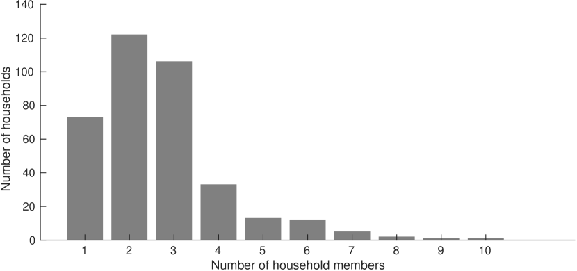
Figure 1: Figure shows the final size data (grey bars) as frequency distribution of total number of cases stratified by household size.

Figures 2 and 3 shows how well the models describe the (marginal distributions of) the observed data. The grey bars in each figure represent the number of observed cases in the influenza data while the error bars represent the final sizes predicted by the model for all the modelling assumptions (see legend at bottom axes of Figure 2). Figure 2 shows the output by household size while Figure 3 shows the results by co-variates. We have further stratified the model fit in Fig. 3 by households size (see Supplementary Figs. S1 to S7). The results reveal that the models do fit well to the marginal household size distributions for all the co-variates.

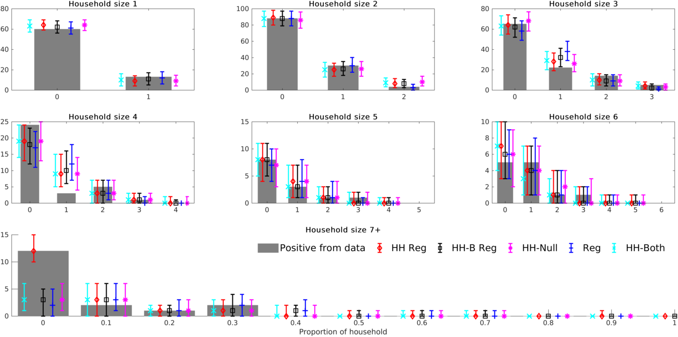
Figure 2: Figure shows the final size data (grey bars) as frequency distribution of total number of cases stratified by household size.

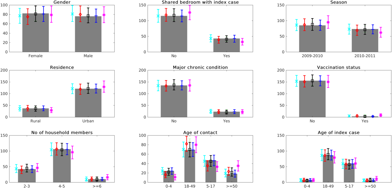
Figure 3: Figure shows the final size data (grey bars) as frequency distribution of total number of cases stratified by co-variates.

Table 1 shows the estimated model parameters and their $95\%$ confidence intervals for all the five modelling assumptions. The values to the right of the CI intervals are the individual covariate p-values from the Wald test. From the table, the co-variate whose p-value indicates significance across all the models is $b_{1}$, which is household contacts in children under 5 years. It is also clear that gender ($b_{12}$) is not statistically significant across all the models. The rest of the parameters have significance that is dependent on the model selected. From the AIC, which is a measure of the relative goodness of fit, the best fitting model is HH-Both. This model has $b_{1}$ and $b_{14}$ (participant having received flu vaccine) being statistically significant. The bottom row shows the p-values from the hypothesis test of the HH-Null model $(H_{0})$ against the other three nested models that have the regression model attached to the transmission parameters. Observations of the table show that the unified models (HH-$\lambda$, HH-$\Lambda$, HH-Both) have advantages over the HH-Null model leading to such small p-values being observed. We can therefore reject the Null model which assumes that within- ($\lambda$) and between- ($\Lambda$) household transmission probabilities do not depend on individual or household level co-variates.

4 Discussion

When a certain outcome is dependent on a number of factors that can be measured or imputed, this is a problem that properly renders itself to regression analysis. Traditional regression analysis, however, assumes independence between observations and this is usually not the case especially in infectious disease transmission where sharing a common environment with an infected person can elevate ones risk of contracting the infection. For example, a recent modelling study [24] using time resolved RSV infection data for RSV found evidence that there might be some niche (household) separation for the two RSV groups explaining how the two groups are able to co-exist together within the same epidemic. This is of course coupled with other factors such as weak cross immunity, differential susceptibility and household composition.

To account for the dependence between observations, multi-level models have been proposed and successfully used in various applications [19]. However, multi-level models are usually unable to capture the feedback relationships that sometimes exist between predictors and outcomes.

In this paper, we explore a dependent-outcome generalised linear model that aims to better detect re-infections probabilities than the standard single level linear models typically carried out. This is done by fusing a disease transmission stochastic model that acts at the group level and then linking disease transmission potential to individual characteristics using a regression model. The stochastic contagion model presented offers a flexible statistical tool for modelling infectious diseases for which the final size data is available. It has an advantage that it makes use of a variable infectious period whereas most previous work have incorporated a constant period or adopted an assumption of an exponential distribution. The infectious period is generalised in our current model so long as the Laplace transform can be specified. In our case, we posited a gamma distribution as a good approximation and evidence from previous simulation studies support our choice [1, 21, 22].

As we are introducing a method rather than testing specific biological hypotheses, we proposed various indicative scenarios for linking co-variates to rates in section 2.1.3. We incorporated the regression on the within household transmission (HH-$\lambda$), between household transmission (HH-$\Lambda$), on both between and within households transmission (HH-Both) or we did not incorporate regression (HH-Null). In all scenarios, the unified transmission-dynamic models performed better, as measured by their p-values, see bottom row 1, compared to the Null model (HH-Null).

As explained by the AIC, the model that best describes the data is HH-Both which governs both the within and between household disease transmission, an observation which is also supported by the statistical test. The next best model is HH-$\Lambda$. A potential explanation why both of these perform better than HH-$\lambda$ is that the covariates in the data are best associated with explaining between household transmission potential.

Our study is not without limitations. While the modelling framework is flexible enough to accommodate a risk of within-household infection that is dependent on both the susceptibility profile of the contacted person and the infectivity profile of the infectious contact, due to limited data for estimating the model parameters, we assumed variable susceptibility and fixed infectivity so that we have $n\times 1$ rather than $n\times n$ within household transmission rate $\lambda$. A future extension would be to have both variable susceptibility and infectivity.

While AIC is perhaps one of the more popular tools for model selection, and included in this work for completeness, it would seem inadequate by itself given that it relies on having independent data or else its asymptotic properties breakdown. We have therefore augumented AIC with the Wald’s W test for model selection and this seems, so far, to be the best model selection method for household epidemic data with correlated outcomes. However, standard methods for model selection could be employed if it can be shown that the dependence is weak, particularly if the number of households, $m$, in the data is large (note that dependence is of order $1/m$ [27]). In our case, this can not be justified.

In conclusion, our analysis shows that accounting for group dependence using a disease transmission model coupled with a regression model improves the predictive utility of the framework over the standard linear model. As such we hope to have aided the design of study analysis plans where the assumption of independence between observations does not hold and where dependence is mechanistically linked, e.g. through close contacts, justifying a stochastic contagion model.

Table 1: Estimated model parameters, their (95% CIs) and their p-values.

$\boldsymbol{\vartheta}$	HH-$\lambda$	HH-$\Lambda$	HH-Both	HH-Null	Reg
$\Lambda$	0.948(0.925, 0.971)	-	-	0.948(0.912 0.983)	-
$\lambda$	-	0.059(0.026, 0.091)	-	0.096(0.058 0.134)	-
$\theta$	2.49(2.1, 2.89)	26.24(25.833, 26.643)	7.502(6.251, 8.754)	7.28(7.251 7.301)	-
$\alpha$	1.136(0.815, 1.456)	1.278(0.912, 1.644)	1.408(1.104, 1.712)	1.088(0.82 1.356)	-
$b_{0}$	$-$5.196($-$5.487, $-$4.905) $<$0.00001	$-$4.34($-$4.633, $-$4.048) 0.035	$-$4.247($-$4.618, $-$3.876)0.12	-	$-$3.258($-$4.52, $-$2.135)$<$0.00001
$b_{1}$	2.837(2.39, 3.284) $<$0.00001	2.221(1.907, 2.536) $<$0.00001	2.387(2.101, 2.672)0.02	-	1.723(1.07, 2.4)$<$0.00001
$b_{2}$	1.03(0.703, 1.357) $<$0.00001	0.647(0.368, 0.927) 0.38	0.471(0.19, 0.751)0.75	-	0.44($-$0.102, 1.029)0.13
$b_{3}$	1.619(1.253, 1.984) $<$0.00001	1.585(1.251, 1.919) 0.051	1.638(1.334, 1.942)0.26	-	1.149(0.568, 1.773)0.0002
$b_{4}$	0.987(0.622, 1.353) $<$0.00001	0.018($-$0.278, 0.314) 0.66	0.485(0.217, 0.752)0.38	-	0.601($-0.56$, 1.797)0.31
$b_{5}$	0.928(0.598, 1.258) $<$0.00001	0.506(0.19, 0.822) 0.71	0.317(0.003, 0.631)0.87	-	0.421($-$0.374, 1.4)0.34
$b_{6}$	0.974(0.636, 1.311) $<$0.00001	0.454(0.128, 0.78) 0.48	0.474(0.161, 0.786)0.78	-	0.532($-$0.306, 1.546)0.25
$b_{7}$	1.066(0.596, 1.535) $<$0.00001	0.501(0.085, 0.917) 0.079	0.606(0.27, 0.943)0.52	-	0.433($-$0.061, 0.885)0.071
$b_{8}$	0.926(0.598, 1.255) $<$0.00001	1.359(0.983, 1.735) 0.028	0.882(0.633, 1.132)0.53	-	0.825(0.13, 1.608)0.027
$b_{9}$	1.383(1.043, 1.724) $<$0.00001	1.347(1.021, 1.673) 0.33	0.9(0.619, 1.182)0.69	-	0.861(0.25, 1.585)0.01
$b_{10}$	$-$0.72($-$1.079, $-$0.361) $<$0.00001	$-$0.575($-$0.933, $-$0.217) 0.72	$-$0.436($-$0.89, 0.017)0.86	-	$-$0.42($-$0.795, $-$0.022)0.034
$b_{11}$	$-$0.557($-$0.93, $-$0.182) $<$0.00001	$-$0.481($-$0.837, $-$0.126) 0.64	$-$0.451($-$0.856, $-$0.047)0.82	-	$-$0.453($-$0.795, $-$0.11)0.0092
$b_{12}$	$-$0.224($-$0.764, 0.315) 0.15	0.147($-$0.287, 0.581) 0.89	$-$0.015($-$0.392, $-$0.361)0.99	-	0.119($-$0.198, 0.437)0.46
$b_{13}$	1.1(0.6, 1.59) $<$0.00001	0.7(0.373, 1.028) 0.29	0.835(0.542, 1.127)0.53	-	0.582(0.194, 0.953)0.0029
$b_{14}$	$-$10.995($-$218.166, 196.177) 0.69	$-$10.998($-$259, 237) 0.85	$-$0.96($-$1.21, $-$0.71)0.016	-	$-$1.164($-$2.592, $-$0.135)0.056
AIC	833.84	817.74	810.16	846.80	826.27
p-value	$<$0.00001***	$<$0.00001***	$<$0.00001***	$H_{0}$	-

References

- [1] C. L. Addy, I. M. Longini Jr., and M. Haber. A Generalized Stochastic Model for the Analysis of Infectious Disease Final Size Data. Biometrics, 47(3):961–974, 1991.
- [2] H. Akaike. A new look at the statistical model identification. IEEE Transactions on Automatic Control, 19(6):716–723, 1974.
- [3] R. Anderson and R. May. Vaccination and herd immunity to infectious diseases. Nature, 318:323–329, 1985.
- [4] R. M. Anderson and R. M. May. Infectious diseases of humans : dynamics and control. Oxford University Press, Oxford; New York, 1991.
- [5] N. T. J. Bailey. The Mathematical Theory of Epidemics. Griffin, London, 1957.
- [6] F. Ball. A Unified Approach to the Distribution of Total Size and Total Area under the Trajectory of Infectives in Epidemic Models. Advances in Applied Probability, 18(2):289–310, 1986.
- [7] F. Ball, D. Mollison, and G. Scalia-Tomba. Epidemics with Two Levels of Mixing. The Annals of Applied Probability, 7(1):46–89, 1997.
- [8] A. J. Black, T. House, M. J. Keeling, and J. V. Ross. The effect of clumped population structure on the variability of spreading dynamics. Journal of Theoretical Biology, 359:45–53, 2014.
- [9] C. R. Brown, J. M. Mccaw, E. J. Fairmaid, L. E. Brown, K. Leder, M. Sinclair, and J. Mcvernon. Factors associated with transmission of influenza-like illness in a cohort of households containing multiple children. Influenza and other Respiratory Viruses, 9(5):247–254, 2015.
- [10] A. Bryk and S. Raudenbush. Hierarchical linear models: applications and data analysis methods. SAGE, London, 1992.
- [11] I. Casado, I. Martinez-Baz, R. Burgui, F. Irisarri, M. Arriazu, F. Elia, A. Navascues, C. Ezpeleta, P. Aldaz, and J. Castilla. Household transmission of influenza A(H1N1)pdm09 in the pandemic and post-pandemic seasons. PLoS ONE, 9(9), 2014.
- [12] S. Cauchemez, A. Bhattarai, T. L. Marchbanks, R. P. Fagan, S. Ostroff, N. M. Ferguson, D. Swerdlow, S. V. Sodha, M. E. Moll, F. J. Angulo, R. Palekar, W. R. Archer, and L. Finelli. Role of social networks in shaping disease transmission during a community outbreak of 2009 H1N1 pandemic influenza. Proceedings of the National Academy of Sciences, 108(7):2825–2830, 2011.
- [13] S. Cauchemez, F. Carrat, C. Viboud, a. J. Valleron, and P. Y. Boëlle. A Bayesian MCMC approach to study transmission of influenza: application to household longitudinal data. Statistics in medicine, 23(22):3469–87, nov 2004.
- [14] D. Colquhoun. An investigation of the false discovery rate and the misinterpretation of p-values. Royal Society Open Science, 1(3):140216, 2014.
- [15] D. Cox and D. Hinkley. Theoretical statistics. Chapman and Hall, London, 1974.
- [16] D. Cox and E. Snell. Analysis of Binary Data. Chapman and Hall, New York, 2 edition, 1989.
- [17] N. Demiris and P. D. O’Neill. Bayesian inference for stochastic multitype epidemics in structured populations via random graphs. Journal of the Royal Statistical Society B, 67:731–745, Jan 2005.
- [18] J. Dennis and R. Schnabel. Numerical methods for unconstrained optimization and nonlinear equations. Society for Industrial and Applied Mathematics, Philadelphia, 1996.
- [19] A. V. Diez-Roux. Multilevel Analysis in Public Health Research. Annual Review of Public Health, 21(1):171–192, 2000.
- [20] D. Hosmer, S. Lemeshow, and R. Sturdivant. Applied Logistic Regression. John Wiley & Sons, Hoboken, 3 edition, 2013.
- [21] T. House, N. Inglis, J. V. Ross, F. Wilson, S. Suleman, O. Edeghere, G. Smith, B. Olowokure, and M. J. Keeling. Estimation of outbreak severity and transmissibility: Influenza A(H1N1)pdm09 in households. BMC medicine, 10(1):117, jan 2012.
- [22] M. J. Keeling and P. Rohani. Modeling Infectious Diseases in Humans and Animals. Princeton University Press, 2007.
- [23] T. Kinyanjui, J. Middleton, S. Guttel, J. Cassel, J. Ross, and T. House. Scabies in residential care homes: Modelling inference and interventions for well-connected population sub-units. PLoS Computational Biology, 14(3), 2018.
- [24] I. K. Kombe, P. K. Munywoki, M. Baguelin, D. J. Nokes, and G. F. Medley. Model-based estimates of transmission of respiratory syncytial virus within households. Epidemics, (December):1–11, 2018.
- [25] L. L. H. Lau, H. Nishiura, H. Kelly, D. K. M. Ip, G. M. Leung, and B. J. Cowling. Household transmission of 2009 pandemic influenza A (H1N1): A systematic review and meta-analysis. Epidemiology, 23(4), 2012.
- [26] P. McCullagh. Regression models for ordinal data. Journal of the Royal Statistical Society. Series B (Methodological), 42(2):109–142, 1980.
- [27] L. Shaw. SIR epidemics in a population of households. PhD thesis, The University of Nottingham, 2016.
- [28] T. Shi, E. Balsells, E. Wastnedge, R. Singleton, Z. A. Rasmussen, H. J. Zar, B. A. Rath, S. A. Madhi, S. Campbell, L. C. Vaccari, L. R. Bulkow, E. D. Thomas, W. Barnett, C. Hoppe, H. Campbell, and H. Nair. Risk factors for respiratory syncytial virus associated with acute lower respiratory infection in children under five years: Systematic review and meta–analysis. Journal of Global Health, 5(2), 2015.
- [29] T. Snidjer and R. Bosker. Multilevel analysis : an introduction to basic and advanced multilevel modeling. SAGE, London, 2 edition, 2012.
- [30] T. K. Tsang, L. L. H. Lau, S. Cauchemez, B. J. Cowling, H. K. Special, and A. Region. Household transmission of influenza virus. 24(2):123–133, 2017.