Decision Propagation Networks for Image Classification

Abstract

High-level (e.g., semantic) features encoded in the latter layers of convolutional neural networks are extensively exploited for image classification, leaving low-level (e.g., color) features in the early layers underexplored. In this paper, we propose a novel Decision Propagation Module (DPM) to make an intermediate decision that could act as category-coherent guidance extracted from early layers, and then propagate it to the latter layers. Therefore, by stacking a collection of DPMs into a classification network, the generated Decision Propagation Network is explicitly formulated as to progressively encode more discriminative features guided by the decision, and then refine the decision based on the new generated features layer by layer. Comprehensive results on four publicly available datasets validate DPM could bring significant improvements for existing classification networks with minimal additional computational cost and is superior to the state-of-the-art methods.

1 Introduction

Image classification [2, 5, 12, 25, 36, 45, 47, 50], aiming at classifying an image into one of several predefined categories, is an essential problem in computer vision. In the last few decades, researchers focus on representing images with hand-crafted low-level descriptors [7, 27], and then discriminating them with a classifier (e.g., SVM [6] or its variants [29, 30]). However, due to the lack of high-level features, the performance is saturating. Thanks to the availability of huge labeled datasets [28, 37] and powerful computational infrastructures, convolutional neural networks (CNNs) could automatically extract discriminative high-level features from the training images, significantly improving the state-of-the-art performance.

Although high-level features are more discriminative, adopting them alone to classify images is still challenging, since with a growing number of categories, the possibilities of confusion increase. In addition, features in the early layers are proved to be able to separate groups of classes in a higher hierarchy [4]. Therefore, researchers attempt to combine high and low-level features together to exploit their complementary strengths [52]. However, a simple combination of them will make the features in relatively high dimensions, hindering practical use.

Other researchers employ low-level features to make coarse decisions and then utilize high-level features to make finers, based on the idea of divide-and-conquer. This could be achieved by designing deep decision trees that implement traditional decision trees [35] with CNNs. With the hierarchical structure of categories, a straightforward way is to make the networks of the root node to identify the coarsest category, and then dynamic route to the networks of a child node to determine the finer one recursively [22]. However, hierarchical information of categories is not always available, therefore researchers are required to design suitable division solutions, making the training process extremely complex (e.g., multiple-staged). Besides, current deep decision tree based methods also face two other fatal weaknesses: (1) the network should save all the tree branches, making the number of parameters explosively larger than a single classification network; (2) once the decision routes to a false path, it could be hardly recovered.

To resolve the above issues, we propose a novel Decision Propagation Module (DPM). The key idea is that if we adopt the early layer to generate a category-coherent decision, and then propagate it along the network, the latter layers could be guided to encode more discriminative features. By stacking a collection of DPMs into the backbone network architectures for image classification, the generated Decision Propagation Networks (DP Nets) are explicitly formulated as to progressively encode more descriptive features guided by the decisions made by early layers and then refine the decisions based on the new generated features iteratively. In the view of residual learning [17], it is much easier to optimize the refining process than to optimize the making of a unreferenced new decision from scratch. Besides the advantage of easier optimization, the property of DPM enables DP Nets to overcome the weaknesses of common deep decision trees naturally. Firstly, in contrast to dynamically routing between several different branches after making a decision, DPM applies the decision as a conditional code to the latter layers similar to [31], such that it could be propagated without bringing additional network branches. Thanks to our novel decision propagation scheme again, DP Nets could be recovered from some false decisions made before as without routing. Furthermore, instead of designating what each intermediate decision indicates explicitly, with weak supervision provided by three novel loss functions, DPM could automatically learn a more suitable and coherent division to separate the categories instead of following the man-made category hierarchy and could be trained in a totally end-to-end fashion with the backbone networks. In total, our contribution is three fold:

• We design a novel DPM, which could propagate the decision made upon an early layer to guide the latter layers.

• We propose three novel loss functions to enforce DPM to make category-coherent decisions.

• We demonstrate a general way to integrate DPMs into various backbone networks to form DP Nets.

Extensive comparison results on four publicly available datasets validate DPM could consistently improve the classification performance, and is superior to the state-of-the-art methods. Code will be made public upon paper acceptance.

2 Related Work

Category Hierarchy, which indicates categories form a semantic hierarchy consisting of many levels of abstraction, has been well exploited [16, 38, 46]. Deng et al. [10] introduced hierarchy and exclusion graphs that capture semantic relations between any two labels to improve classification. Yan et al. [51] proposed a two-level hierarchical CNN with the first layer separating easy classes using a coarse category classifier and the second layer handing difficult classes utilizing fine category classifiers. To mimic the high level reasoning ability of human, Goo et al. [14] introduced a regulation layer that could abstract and differentiate object categories based on a given taxonomy, significantly improving the performance. However, the man-made category hierarchy may be not a good division in the view of CNNs.

Deep Decision Trees/Forests.   The cascade of sample splitting in decision trees has been well explored by traditional machine learning approaches [35]. With the rise of deep networks, researchers attempt to design deep decision trees or forests [54] to solve the classification problem. Since prevailing approaches for decision tree training typically operate in a greedy and local manner, hindering representation training with CNNs, Kontschieder et al. [22] therefore introduced a novel stochastic routing for decision trees, enabling split node parameter learning via backpropagation. Without requiring the user to set the number of trees, Murthy et al. [32] proposed a “data-driven” deep decision network which stage-wisely introduces decision stumps to classify confident samples and partition the remaining data, which is difficult to classify, into smaller data clusters for learning successive expert networks in the next stage. Ahmed et al. [1] further proposed to combine the learning of a generalist to discriminate coarse groupings of categories and the training of experts aimed at accurate recognition of classes within each specialty together and obtained substantial improvement. Instead of clustering data based on image labels, Chen et al. [8] proposed a large-scale unsupervised maximum margin clustering technique to split images into a number of hierarchical clusters iteratively to learn cluster-level CNNs at parent nodes and category-level CNNs at leaf nodes.

Different from the above approaches that implement each decision branch with another separate routing network, Xiong et al. [49] proposed a conditional CNN framework for face recognition, which dynamic routes via activating a part of kernels, making the deep decision tree more compact. Based on it, Baek et al. [3] proposed a fully connected “soft” decision jungle structure to enable the decision could be recoverable, and thus lead to more discriminative intermediate representations and higher accuracies.

Our DPM could be considered as a deep decision tree based approach, and the most similar work to ours is [3]. However, the difference is at least three-fold. Firstly, instead of dynamic activating a part of kernels to reduce parameters which would make each kernel work for only a part of decisions, our DPM, which adopts conditional codes to propagate decisions, could enforce each kernel to work for all the decisions, and thus make full use of the neurons. Secondly, their approach requires layers with channel number larger than the category number, which could be hardly satisfied in real cases with 1k or more categories, while our solution does not have such restriction. Last but not least, we designed three novel loss functions to enforce DPM could make category-coherent decisions.

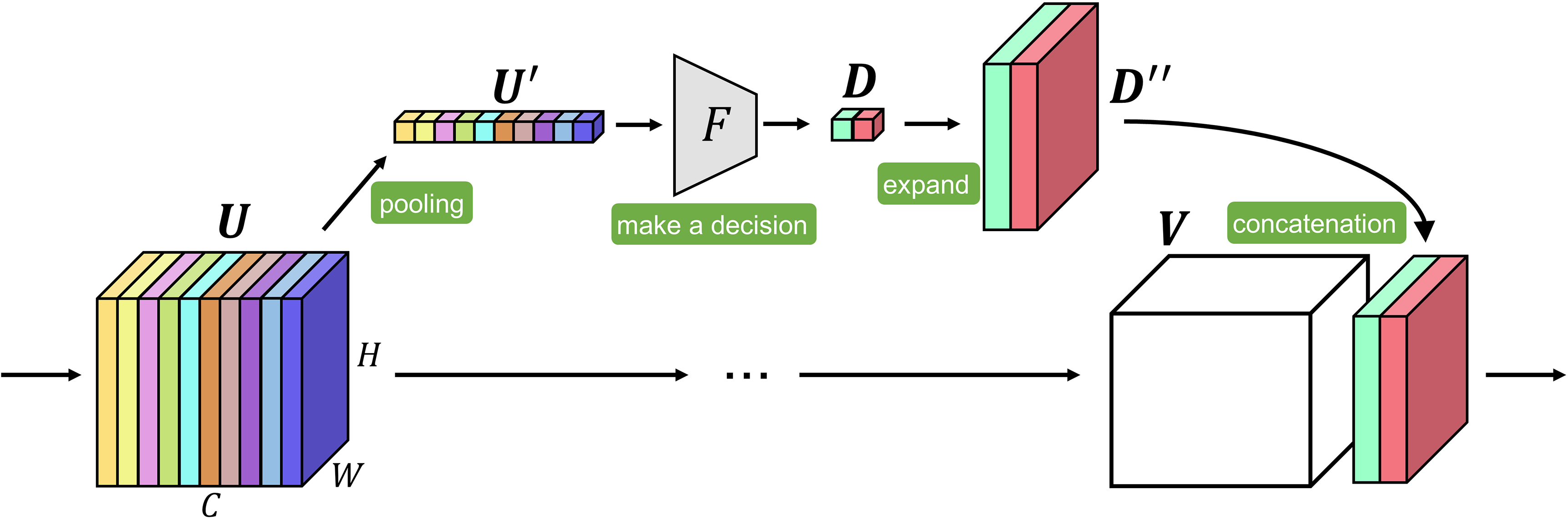
Figure 1: The demonstration of Decision Propagation Module: given a feature map ${\bf{U}}$, we first conduct global average pooling to obtain the pooled feature ${\bf{U^{{}^{\prime}}}}$; and then classify it using the network layer ${{F}}$ to get an immediate decision ${\bf{D}}$; finally the decision is expanded and concatenated with the feature map ${\bf{V}}$. Note that, ${\bf{V}}$ could be ${\bf{U}}$ or any other subsequent feature map.

Belief Propagation in CNNs.   Belief propagation has been well studied for a long time especially by traditional methods [9, 13]. Actually, the concept of belief propagation has also been exploited by various deep networks. Highway networks [41] allow unimpeded information propagates across several layers on information highways. ResNets [19] propagate the identities via the well-defined res-block structures. Compared with those skip-connection based methods that propagate the identity feature maps directly, the intermediate decisions propagated by our approach are in relatively lower dimensions but with more explicit (category-coherent) guidance. Therefore, our designed DPM could be considered as another feasible solution for belief propagation. Besides, we will also see that DPM could be easily integrated into skip-connection based networks to further improve their performance.

3 Decision Propagation Networks

In this section, we will first define what is the category-coherent decision, and then introduce the structure of Decision Propagation Module (DPM) together with three corresponding loss functions for training it; in addition, we will discuss the large category issue that hinders DPM training and our solution; finally we will demonstrate several exemplars of Decision Propagation Networks by integrating DPMs into some popular backbone network architectures.

3.1 The Category-coherent Decision

Given inputs with the same object category, if their corresponding decisions are similar, then these decisions could be called the category-coherent decisions. Note that, we also allow inputs with multiple categories to have the same decision results. In this paper, we set the category-coherent decision with $n$ ($n\leq N$) auxiliary categories, namely ${\bf{D}}=\left(D_{1},...,D_{n}\right)$, and $D_{1}+D_{2}+...+D_{n}=1$.

3.2 Structure of Decision Propagation Module

The Decision Propagation Module (DPM) is a computational unit that is devised to make a category-coherent early decision [53] based on the features encoded in an early layer and then propagate it to the following network layers to guide them. A diagram of DPM is shown in Fig. 1.

3.2.1 Make a Soft Decision

Give an intermediate feature map ${\bf{U}}$ (${\bf U}$ $\in\mathbb{R}^{C\times H\times W}$) , our aim is to make a category-coherent decision to guide subsequent network layers without bringing too much additional computational cost. Therefore, instead of continuing convolving on it, we propose to adopt global average pooling (GAP) to extremely reduce the feature dimensions. As verified in [26], the pooled feature map ${\bf{U^{{}^{\prime}}}}$ with channel-wise statistics, is usually discriminative enough for classification. We thus adopt a fully connected network $F$ with one or two layers to make a decision based on it. To facilitate this decision branch could be optimized with the whole network structure in an end-to-end manner, we apply the softmax function to the output, and thus obtain a “soft” decision ${\bf{D}}$.

3.2.2 Decision Propagation

To make use of the information aggregated in the intermediate decision ${\bf{D}}$, a straightforward idea is to dynamic route accordingly [32], making the network to form a deep decision tree. As a deep decision tree will bring explosive parameter increment and could not be recovered from previous false decisions, we thus follow [31] and consider the intermediate decision as a conditional code, such that the category prediction process could be directed by conditioning on it. Specifically, we expand the decision vector $\bf{D}~{}(\bf{D}\in\mathbb{R}^{n})$ to be with the same resolution as the feature map of ${\bf{V}}$, by copying the decision scores directly, and then concatenate the expanded decision ${\bf{D^{{}^{\prime\prime}}}}~{}({\bf{D^{{}^{\prime\prime}}}}\in\mathbb{R}^{n\times H\times W})$ with ${\bf{V}}$ as additional channels (see Fig. 1). Note that, ${\bf{V}}$ could be ${\bf{U}}$ itself or any other feature map outputted by a subsequent network layer, and we also allow propagating one decision to multiple layers.

3.3 Loss Functions for DPM

To enable DPM to make category-coherent decisions, we propose three novel loss functions to guide it. In the following, we will describe them one by one.

Notations.   We denote $\mathcal{D}~{}(\mathcal{D}\in\mathbb{R}^{b\times n})$ as all the ${\bf{D}}$s in a mini-batch with size of $b$, where $\mathcal{D}_{kj}$ is the decision score (confidence) of the $j$-th auxiliary category for the $k$-th instance in the batch.

Decision Explicit Loss.   If the intermediate decision made by DPM is ambiguous, the following layers could hardly get any useful information from it. Therefore, we introduce a decision explicit loss to encourage the decision score of one or several auxiliary categories to have relatively larger values, while avoiding all the auxiliary categories to have similar scores. The loss function is defined as follows:

$$L_{explicit}({\bf{\mathcal{D}}})=\frac{1}{b}\sum_{k\in\{1...b\}}\left(-\sum_{j\in\{1...n\}}{\mathcal{D}_{kj}\log{\mathcal{D}_{kj}}}\right),$$ (1)

which is in the form of entropy to encourage the decision scores of different auxiliary categories to vary a lot.

Decision Consistent Loss.   Simply enforcing the decision to be explicit is not enough. Besides, we wish the decisions for many different instances with the same original category should be consistent. Specifically, their decision scores of the same auxiliary category should be similar.

Therefore, we propose a decision consistent loss which is defined as follows:

$$L_{consistent}({\bf{\mathcal{D}}})=\frac{1}{Nn}\sum_{i\in\{1...N\}}\sum_{j\in\{1...n\}}\mathcal{V}_{ij},$$ (2)

where $\mathcal{V}_{ij}$ is the sample variance of those $\mathcal{D}_{kj}$ $(k\in\{1...b\})$ for the instances whose original category is $i$ in the batch.

Denote $\mathcal{I}~{}(\mathcal{I}\in\mathbb{R}^{b\times N})$ as the indicator matrix for a batch of data: if the original category of the $k$-th instance in the batch is $i$, then $\mathcal{I}_{ki}=1$; otherwise $\mathcal{I}_{ki}=0$. Thus the mean decision score $\mathcal{M}_{ij}$ of the $j$-th auxiliary category for all the instances in the batch with original category $i$ could be calculated with the following equation:

$$\mathcal{M}_{ij}=\frac{\sum_{k\in\{1...b\}}\left(\mathcal{I}_{ki}\mathcal{D}_{kj}\right)}{\sum_{k\in\{1...b\}}\mathcal{I}_{ki}+\delta},$$ (3)

where $\delta$ is a small value to avoid divide-zero error. After that, we could calculate $\mathcal{V}_{ij}$ with

$$\mathcal{V}_{ij}=\frac{\sum_{k\in\{1...b\}}\mathcal{I}_{ki}{\left(\mathcal{D}_{kj}-\mathcal{M}_{ij}\right)}^{2}}{\sum_{k\in\{1...b\}}\mathcal{I}_{ki}-1+\delta}$$ (4)

By substituting Equation 3 into Equation 4 and expand the formulation, we obtain a new equation:

$$\mathcal{V}_{ij} =\frac{\sum_{k\in\{1...b\}}\mathcal{I}_{ki}{\mathcal{D}_{kj}}^{2}}{\sum_{k\in\{1...b\}}\mathcal{I}_{ki}-1+\delta}$$ (5)

$$-\frac{{\left(\sum_{k\in\{1...b\}}{\mathcal{I}_{ki}{\mathcal{D}_{kj}}}\right)}^{2}}{{\left(\sum_{k\in\{1...b\}}\mathcal{I}_{ki}+\delta\right)}{\left(\sum_{k\in\{1...b\}}\mathcal{I}_{ki}-1+\delta\right)}}$$

However, calculating those $\mathcal{V}_{ij}$ one by one is very time-consuming, we therefore leverage matrix operations to accelerate them. The derived equation is as follows:

$$\mathcal{V}=\frac{{\mathcal{I}}^{\mathrm{T}}\times\left(\mathcal{D}\mathcal{D}\right)}{\mathcal{I}^{{}^{\prime}}-1}-\frac{\left({\mathcal{I}}^{\mathrm{T}}\times\mathcal{D}\right)\left({\mathcal{I}}^{\mathrm{T}}\times\mathcal{D}\right)}{\mathcal{I}^{{}^{\prime}}\left(\mathcal{I}^{{}^{\prime}}-1\right)},$$ (6)

which is a matrix with the value in $i$-th row and $j$-th column to be $\mathcal{V}_{ij}$, namely $\mathcal{V}\in\mathbb{R}^{N\times{n}}$. Operator $\times$ indicates cross-product, while all other operations are conducted element-wisely. $\mathcal{I}^{{}^{\prime}}\in\mathbb{R}^{N\times n}$ is a two dimension matrix with $\mathcal{I}^{{}^{\prime}}_{ij}=\sum_{k\in\{1...b\}}\mathcal{I}_{ki}+\delta$, for arbitrary $j\in\{1...n\}$. Although simple, it is critical for training the module in an efficient mode.

Decision Balance Loss.   Besides the above two losses, we also propose a decision balance loss to avoid the degraded situation that no matter what original category the input instance is, DPM explicitly assign it to a single auxiliary category. Therefore, the decision balance loss is to encourage all auxiliary categories could be balanced assigned, in the form of the reverse of entropy:

$$\begin{split}L_{balance}({\bf{\mathcal{D}}})&=\sum_{j\in\{1...n\}}m_{j}\log m_{j},\\ m_{j}&=\sum_{k\in\{1...b\}}\mathcal{D}_{kj}+\delta.\end{split}$$ (7)

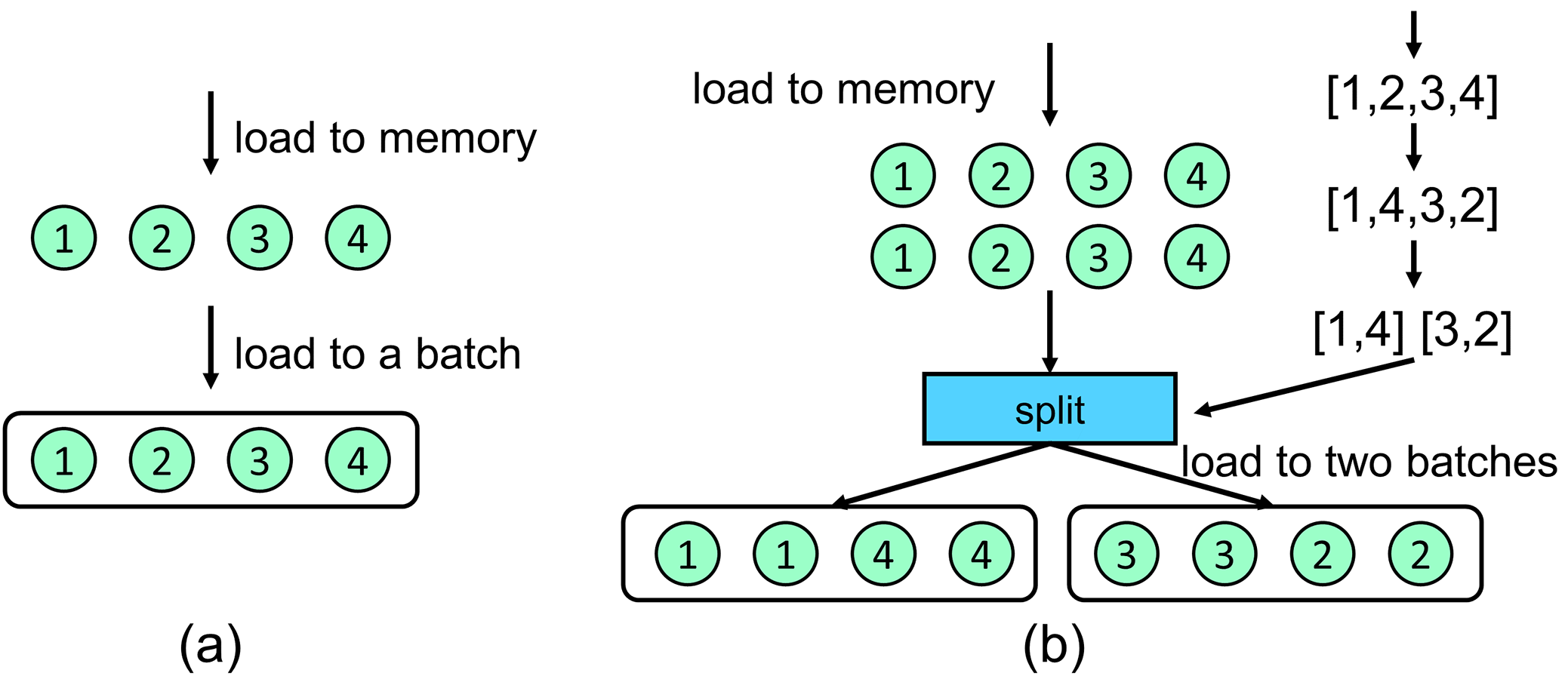
Figure 2: The demonstrations of loading data with 4 categories (the circle with digit $i$ inside indicates an instance whose original category is $i$) into a batch whose size is 4: (a) traditional approach will results in the number of instances with each category in a training batch is only one; (b) our approach that loads more data samples into memory, and shuffles then splits the samples into multiple batches could increase the number of instances that are with the same categories in each training batch.

3.4 Large Category Issue

For all the original categories appear in a batch, we expect their decision scores could be consistently, explicitly and balancedly distributed into all the auxiliary categories. However, due to the limitation of computational resources and the training issues of large batch SGD [15], the batch size is normally set with a small number between 1 to 256. For the tasks with 100, 1000 or even more original categories, randomly load a batch of data will result in the number of instances with each original category is only two or even smaller, resulting in $L_{consistent}$ could not work.

Therefore, instead of simply increasing the batch size to maintain more data samples, we propose a novel load-shuffle-split strategy which could resolve the large category issue without enlarging the batch size significantly. Specifically, given Fig. 2 as an example, where the original category number is 4 and the mini-batch size is 4, too. The load-shuffle-split strategy has three key steps: (1) instead of loading 4 data samples only, we load more samples in each iteration (e.g., 8); (2) we first generate a number list $\left[1,2,3,4\right]$ with containing all the category IDs; and then shuffle it to obtain another list $\left[1,4,3,2\right]$; finally the shuffled list is splitted into two lists: $\left[1,4\right]$ and $\left[3,2\right]$; (3) we split the 8 data samples into two training batches according to the category IDs in the two splitted lists generated in the last step (see Fig. 2 again), and then train the two batches separately. In this case, the number of instances with each original category in a training batch is doubled.

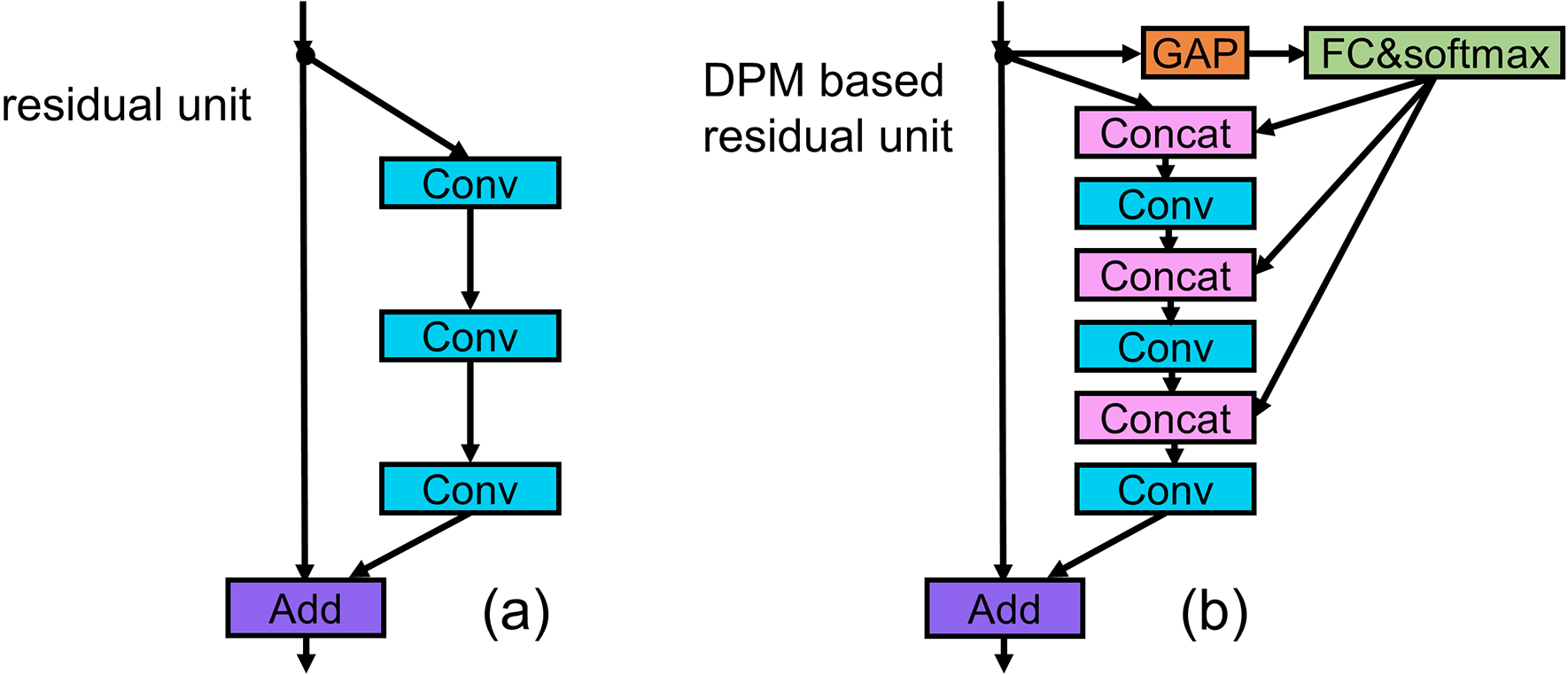
Figure 3: The schema of (a) the original residual unit; and (b) the DPM based residual unit.

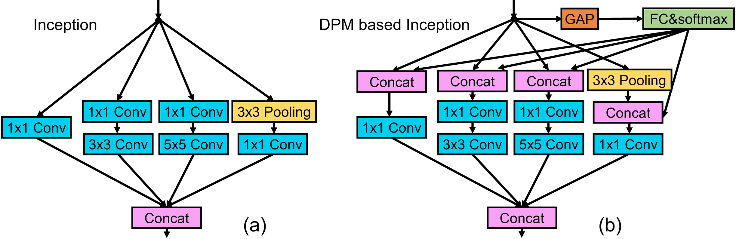
Figure 4: The schema of (a) the original Inception; and (b) the DPM based Inception.

3.5 Exemplar Decision Propagation Networks

Our DPM is very flexible and could be integrated into various classification network architectures to form Decision Propagation Networks (DP Nets). As it is straightforward to apply it to VGG network [39] or AlexNet [24], in this section we only illustrate how to integrate DPMs into modern sophisticated architectures.

For residual networks, we take ResNet [17] as an example. As ResNet is organized by stacking multiple residual blocks, we thus integrate DPM into each residual unit, see Fig. 3 for a demonstration. The intermediate decision is propagated along the residual branch, and thus these neurons could be guided to learn better residuals. For other popular architectures, such as Inception network, we also demonstrate how to integrate DPM into the Inception module in Fig. 4. The integration of DPM(s) with many other ResNet and Inception variants, such as ResNeXt [48], Inception-ResNet [43] could be constructed in similar schemes.

4 Experiments

In this section, we evaluate the image classification performance of our approach on four publicly available datasets. Our main focus is on demonstrating DPM could improve the performance of backbone CNN networks on image classification, but not on pushing the state-of-the-art results. Therefore, we spend more space to compare our approach with popular baseline networks on three relatively small-scale datasets due to limited computational resources, and finally report our results on the ImageNet 2012 dataset [11] to validate the scalability of our approach.

4.1 Implementation

We implement DPM and reproduce all the evaluated networks with PyTorch [34]. The decision network $F$ of DPM is constructed with two fully connected (FC) layers around ReLU [33] and followed with a Softmax layer to normalize the decision scores. To limit the model complexity, we reduce the dimension in the first FC layer with the reduction ratio of 16. For all the DPMs integrated into a network, we assume all their auxiliary category numbers are exactly the same to ease network construction, and we set it with 2 if not specifically stated. For VGG, we add BatchNorm (BN) [21] while with no Dropout [40], and use one FC layer. For Inception, we choose v1 with BN. While other models are identical to the original papers.

4.2 Dataset and Training Details

CIFAR-10 and CIFAR-100 [23] consist of 60k 32$\times$32 images that belong to 10 and 100 categories respectively. We train the models on the whole training set with 50k images in a mini-batch of 128, and evaluate them on the test set. We set the initial learning rate with 0.1, and drop it by 0.2 at 60, 120 and 160 epochs for total 200 epochs. For data augmentation, we pad 4 pixels on each side of the image, and randomly sample a 32$\times$32 crop from the padded image or its horizontal flip, and then apply the simple mean/std normalization.

CINIC-10 [42] contains 270k 32$\times$32 images belonging to 10 categories, equally split into three subsets: train, validation, and test. We train the models on the train set with a mini-batch of 128 and evaluate them on the test set. The training starts with an initial learning rate of 0.1, and cosine annealed to zero for total 300 epochs, based on the same data augmentation scheme as in CIFARs.

ImageNet [11] consists of 1.2 million training images and 50k validation images from 1k classes. We train the models with minimal data augmentation including random resized crop, flip and the simple mean/std normalization on the whole training set and report results on the validation set. The initial learning rate is set to 0.1 and decreased by a factor of 10 every 30 epochs to a total of 100 epochs.

During training, the three loss functions are calculated for all the DPMs in the network, and the average of each loss is accumulated with the traditional cross-entropy loss for classification. We set the weighting of the three loss terms to be 0.01 on ImageNet while 0.1 on others. All the models are trained from scratch with SGD using default parameters as the optimizer, and the weights are initialized following [18]. We evaluate the single-crop performance at each epoch and report the best one.

4.3 CIFAR and CINIC-10 Experiments

To evaluate the effectiveness of DPM, we first perform extensive ablation experiments on three relatively small datasets to verify that DP Nets with integrating DPMs outperform the corresponding baseline networks without bells and whistles, and then compare them with the state-of-the-art methods to demonstrate the superiority.

Architecture	#Category per batch	#Images per iter.	Acc (%)
			Top-1	Top-5
ResNet-20	-	-	68.82	91.03
ResNet-20	10	1280	64.88	89.54
DP-ResNet-20	10	1280	65.34	89.87
DP-ResNet-20	25	512	70.51	92.25
DP-ResNet-20	50	256	69.80	91.98
DP-ResNet-20	100	128	69.50	91.69
ResNet-56	-	-	72.23	92.36
ResNet-56	10	1280	54.13	78.65
DP-ResNet-56	10	1280	53.73	78.86
DP-ResNet-56	25	512	73.76	93.39
DP-ResNet-56	50	256	73.58	93.24
DP-ResNet-56	100	128	73.41	93.18

Table 1: Classification results on CIFAR-100 with different numbers of categories in a training batch. #Images per iter. is the number of images that are loaded into memory in each iteration, #category per batch indicates the number of categories that appears in a training batch.

Architecture	#Auxiliary category	Acc (%)
		Top-1	Top-5
DP-ResNet-20	2	70.51	92.52
DP-ResNet-20	5	69.49	91.65
DP-ResNet-20	10	69.91	91.56
DP-ResNet-20	25	69.41	91.67
DP-ResNet-56	2	73.76	93.39
DP-ResNet-56	5	73.86	93.28
DP-ResNet-56	10	73.51	93.32
DP-ResNet-56	25	73.02	92.95

Table 2: Classification results on CIFAR-100 with different number of auxiliary categories for intermediate decisions.

4.3.1 Category Number in Each Batch

As mentioned before, to handle the large category issue that affects the estimation of decision consistent loss, we proposed a load-shuffle-split strategy. In this part, we will evaluate the effects brought by the strategy. Since CIFAR-100 consists of images with 100 categories while the mini-batch size is 128, we thus choose it to investigate. Specifically, we make 4 different configurations, with each configuration has around 128 images in a training batch for fair comparisons.

The results in Tab. 1 show that DP-ResNet-20 and DP-ResNet-56 both obtain the best results when enforcing each training batch with images in 25 categories, instead of the default 100 categories. Therefore we could conclude that our load-shuffle-split strategy is useful for training DP Nets on large category datasets. However, when the number of categories in a training batch keeps decreasing, the performance drops heavily. The reason is that CNNs require the data to be i.i.d. distributed, but the reduction of category number in each batch will hurt the distribution, thus degrading the performance. To validate this, we also conduct experiments on the baseline ResNet-20 and ResNet-56 with 10 categories in each batch and find the performance also drops. Even though, our approach could leverage it to handle the large category issue.

Architecture	Configuration	Acc (%)
		Top-1	Top-5
DP-ResNet-20	w/o $L_{explicit}$	70.31	92.11
DP-ResNet-20	w/o $L_{consistent}$	70.07	92.05
DP-ResNet-20	w/o $L_{balance}$	69.44	91.88
DP-ResNet-20	-	70.51	92.25
DP-ResNet-56	w/o $L_{explicit}$	73.27	93.19
DP-ResNet-56	w/o $L_{consistent}$	73.52	93.15
DP-ResNet-56	w/o $L_{balance}$	72.87	92.73
DP-ResNet-56	-	73.76	93.39

Table 3: Classification results of DP-ResNets on the CIFAR-100 dataset with ablating part of loss functions.

4.3.2 Auxiliary Category Number

To investigate the effects of auxiliary category number in DPM, we follow the best configuration in the above experiments that set the category number in each training batch as 25, and report the experimental results in Tab. 2. It could be seen that the performance with 2 auxiliary categories is very good and stable, while those with larger auxiliary categories vary a lot for the two different models. The reason is probably that current supervision is not enough to enforce DPM to make use of more auxiliary categories. Besides, we will show that it is the decision scores that encode some meaningful information about the original category, rather than the auxiliary category itself (see Sec. 4.3.6). Therefore, we simply choose the auxiliary category number to be 2.

4.3.3 Three Loss Functions

These experiments are to evaluate the influence of each loss function for training DPM by ablating one of them. The results depicted in Tab. 3 show that the performance drops if we ablate any loss function. Particularly, $L_{balance}$ has the largest influence on the classification results and the accuracies drop nearly  1% for both models, which probably indicates DPM is easily degenerated to consistently and explicitly assigning all pooled feature maps into a single auxiliary category. In addition, we would like to point out that DP-ResNets with ablating one loss function could still outperform the baseline networks whose results are reported in Tab. 1, validating the effectiveness of DPM.

Architecture	#params	#MACs	Acc (%)
			CIFAR10	CIFAR-100	CINIC-10
NIN [26]	996.99k	0.22G	89.71	67.76	80.10
DDN [32] *	-	-	90.32	68.35	-
DCDJ [3] *	-	-	-	68.80	-
DP-NIN	997.9k	0.23G	90.87(1.16)	69.11(1.35)	81.07(0.97)
ResNet-56 [17]	855.77k	0.13G	93.62	72.23	84.74
SE-ResNet-56 [20]	861.82k	0.13G	94.28	73.81	85.09
DP-ResNet-56	894.96k	0.14G	94.35 (0.73)	73.76 (1.53)	85.50 (0.76)
ResNet-110 [17]	1.73M	0.26G	93.98	73.94	85.18
SE-ResNet-110 [20]	1.74M	0.26G	94.58	74.42	85.57
DP-ResNet-110	1.81M	0.28G	94.56(0.58)	74.85 (0.91)	86.34 (1.16)
GoogLeNet [44]	6.13M	1.53G	95.27	79.41	87.89
DP-GoogLeNet	6.35M	1.54G	95.65(0.38)	80.73(1.32)	88.31(0.42)
VGG13 [39]	9.42M	0.23G	94.18	74.42	85.04
DP-VGG13	9.49M	0.23G	94.61 (0.43)	74.94 (0.52)	85.59(0.55)

Table 4: Classification results on the CIFAR-10, CIFAR-100 and CINIC-10 datasets. Note that the number of parameters and MACs are calculated based on the experiments on CIFAR-10. The numbers in brackets denote the performance improvement. * indicates the results are reported in the original papers.

4.3.4 Comparisons with the State-of-the-art Methods

We conduct extensive experiments on the three challenging datasets: CIFAR-10, CIFAR-100 and CINIC-10, with various popular architectures, including ResNets [17], Network in Network (NIN) [26], GoogLeNet [44] and VGG [39] as backbones. The results demonstrated in Tab. 4 show that by integrating DPMs, all the networks could consistently obtain significant better performance (e.g., more than 1.5% improvement for DP-ResNet-56 on CIFAR-100), validating the effectiveness and versatility of DPM. Particularly, we would like to point out that DP-ResNet-56 outperforms the original ResNet-110 on both the CIFAR10 and CINIC-10 datasets, but with nearly half the numbers of parameters and multiply-and-accumulates (MACs). In addition, we also compare our approach with two latest decision tree based methods: Deep Convolutional Decision Jungle (DCDJ) [3] and Deep Decision Network (DDN) [32]. Since they have not released their codes, we thus compare ours with the results reported in the original papers. It could be seen that our DP-NIN outperforms DCDJ and DDN with all using NIN as the backbone network. Finally, we compare our DPM with the most advanced SE block [20], whose motivation is to improve the performance of various backbone architectures in the manner of attention. From Tab. 4, we could see that DPM is comparable with the SE block on classification and sometimes is superior to it.

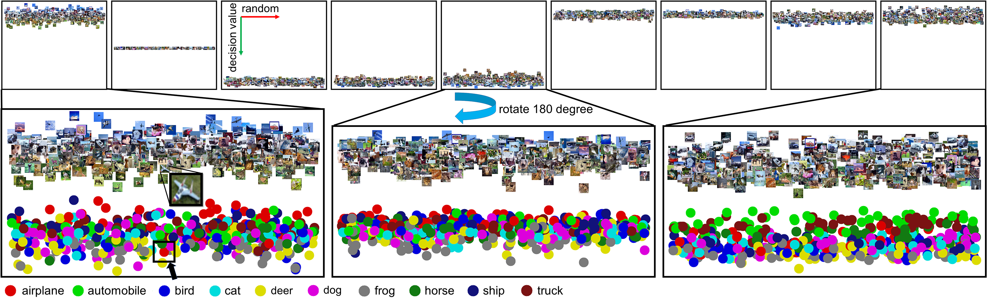
Figure 5: Above row: each column visualizes the decisions made by one (totally 9) DPM of DP-ResNet-20 on 512 images in CIFAR-10 (from left to right: DPM of early layer to the latter layer). The vertical position of each image indicates the decision score: closer to the bottom, larger decision score assigned to the first auxiliary category; while the images are randomly spanned across the horizontal direction. Below row: the zoomed view of the decisions and the corresponding categories represented with colored circles. Note that, the decision scores of the first auxiliary category are concentrated in a small range instead of the whole $\left[0,1\right]$, but we still could see the images are well semantically clustered, especially for the decisions made by the last DPM.

4.3.5 Complexity Analysis

To enable practical use, DPM is expected to provide an effective trade-off between complexity and performance. Therefore, we report the statistics of complexity in Tab. 4. It could be seen that, by integrating DPMs, the increased numbers of parameters and multiply-and-accumulates (MACs) are less than 5% of their original ones. While in several previous subsections, we have validated that the brought improvements are significant. Therefore, we could conclude that the overhead brought by DPM is deserved.

4.3.6 Visualization and Discussion

To investigate what DPM learns, we visualize the decisions made by the 9 DPMs of DP-ResNet-20 on 512 images from the CIFAR-10 dataset in Fig. 5, with DPM of the earliest layer to the latest layer located from left to right in sequence. For the decisions made by each DPM, all 512 images are visualized with their positions related to the decision scores assigned to them: the larger decision score assigned to the first auxiliary category (totally two), the more bottom position the image is located, while all the images are randomly spanned across the horizontal direction. Since with limited supervision, the decision scores are concentrated in a small range instead of the whole $\left[0,1\right]$, but we will show it is enough to distinguish the categories.

We could see the images in the first column are distributed along the vertical direction with “blue” images located in the above, and “green” images in the below, indicating that the first DPM probably makes decisions based on the color information. Although simple, frogs and airplanes are separated quite well, validating that low-level information is useful for classification. The second DPM seems to not work, assigning equal decision scores to the two auxiliary categories. This behavior is similar to ResNet that allows some gated shortcuts to be closed. Interestingly, the 3-5th DPMs make almost reversed decisions (e.g., the score is about one minus the score made by the other DPM), indicating that the auxiliary categories made by different DPMs could be different, and neural networks have the ability to decode these decisions. We rotate the decisions in the 5-th column, and find it is somewhat consistent with the decisions in the first column, but has better semantic clustering along the vertical direction. For example, all the airplanes (see the red circle in Fig. 5) are located in the above part, while a “green” airplane is located in the below part by mistake within the first decisions (see the black rectangle in the first zoomed view in Fig. 5), validating that our approach could be recovered from some false decisions made before. We also visualize the decisions made by the last DPM, and find that the instances with the same categories (e.g., airplane, automobile) are located within a quite small range along the vertical axis and are well separated with some other categories, therefore we could conclude it is the decision score that encodes some meaningful information about the object category, rather than the auxiliary category itself. From the three zoomed views, we could see that the decisions are progressively refined, validating our intuition to propagate decisions. Particularly, trucks and automobiles are located in similar vertical ranges, which could be considered as belonging to a coarse category “man-made objects” mentioned by the category hierarchy. However, other “man-made objects”, such as airplanes and ships, are mixed with the objects belonging to the coarse category “animals”. Therefore, we conclude that the decision made by DPM is not based on the man-made category hierarchy, but another division that is better in the view of CNNs.

Architecture	#Category in a batch	Batch size	Acc(%)
			Top-1	Top-5
ResNet-18	-	256	68.06	88.55
DP-ResNet-18	-	256	68.65	88.83
DP-ResNet-18	250	$\sim$ 1024	69.10	89.03
ResNet-50	-	256	74.42	91.97
DP-ResNet-50	-	256	75.47	92.75
DP-ResNet-50	250	$\sim$ 768	76.15	92.98
GoogLeNet	-	256	70.68	90.08
DP-GoogLeNet	-	256	71.22	90.37
DP-GoogLeNet	250	$\sim$ 1024	71.66	90.54
ResNet-101	-	256	76.66	93.23
DP-ResNet-101	-	256	77.59	93.81
DP-ResNet-101	200	$\sim$ 512	78.21	93.92

Table 5: Classification results on ImageNet.

4.4 ImageNet Experiments

We also evaluate the performance of various DP Nets on ImageNet [11]. The results depicted in Tab. 5 show that DP Nets outperform all the baseline networks with large margins (e.g., $\sim$0.6% for ResNet-18 and GoogLeNet, $\sim$1.0% for ResNet-50 and ResNet-101) that randomly sample all 1000-category instances into a training batch, in which case $L_{consistent}$ could hardly contribute to the training. Therefore, we also conduct experiments with setting batch sizes to be 1024, 768 and 512, while enforcing the category number in a batch to be 250, 250 and 200 using the load-shuffle-split strategy. We could see that the improvements on top-1 accuracy for all DP Nets are finally enlarged to 1.0% - 1.6%, validating the scalability of our approach.

5 Conclusion

We have presented the Decision Propagation Module (DPM), a novel drop-in computational unit that could propagate the category-coherent decision made upon an early layer of CNNs to guide the latter layers for image classification. Decision Propagation Networks generated by integrating DPMs into existing classification networks could be trained in an end-to-end fashion, and bring consistent improvements with minimal additional computational cost. Extensive comparisons validate the effectiveness and superiority of our approach. We hope DPM become an important component of various networks for image classification. In the future, we plan to extend our approach to handle more vision tasks, e.g., detection and segmentation.

References

- [1] Karim Ahmed, Mohammad Haris Baig, and Lorenzo Torresani. Network of experts for large-scale image categorization. In ECCV, pages 516–532, 2016.
- [2] Zeynep Akata, Scott Reed, Daniel Walter, Honglak Lee, and Bernt Schiele. Evaluation of output embeddings for fine-grained image classification. In CVPR, pages 2927–2936, 2015.
- [3] Seungryul Baek, Kwang In Kim, and Tae-Kyun Kim. Deep convolutional decision jungle for image classification. arXiv preprint arXiv:1706.02003, 2017.
- [4] Alsallakh Bilal, Amin Jourabloo, Mao Ye, Xiaoming Liu, and Liu Ren. Do convolutional neural networks learn class hierarchy? IEEE TVCG, 24(1):152–162, 2017.
- [5] Michael Blot, Matthieu Cord, and Nicolas Thome. Max-min convolutional neural networks for image classification. In ICIP, pages 3678–3682, 2016.
- [6] Chih-Chung Chang and Chih-Jen Lin. Libsvm: A library for support vector machines. ACM TIST, 2(3):27, 2011.
- [7] Jie Chen, Shiguang Shan, Chu He, Guoying Zhao, Matti Pietikainen, Xilin Chen, and Wen Gao. Wld: A robust local image descriptor. TPAMI, 32(9):1705–1720, 2009.
- [8] Tao Chen, Shijian Lu, and Jiayuan Fan. Ss-hcnn: Semi-supervised hierarchical convolutional neural network for image classification. IEEE TIP, 28(5):2389–2398, 2018.
- [9] Vincent Conitzer. Designing preferences, beliefs, and identities for artificial intelligence. In AAAI, volume 33, pages 9755–9759, 2019.
- [10] Jia Deng, Nan Ding, Yangqing Jia, Andrea Frome, Kevin Murphy, Samy Bengio, Yuan Li, Hartmut Neven, and Hartwig Adam. Large-scale object classification using label relation graphs. In ECCV, pages 48–64, 2014.
- [11] Jia Deng, Wei Dong, Richard Socher, Li-Jia Li, Kai Li, and Li Fei-Fei. ImageNet: A large-scale hierarchical image database. In CVPR, pages 248–255, 2009.
- [12] Gamaleldin Elsayed, Dilip Krishnan, Hossein Mobahi, Kevin Regan, and Samy Bengio. Large margin deep networks for classification. In NIPS, pages 842–852, 2018.
- [13] Pedro F. Felzenszwalb and Daniel P. Huttenlocher. Efficient belief propagation for early vision. IJCV, 70(1):41–54, 2006.
- [14] Wonjoon Goo, Juyong Kim, Gunhee Kim, and Sung Ju Hwang. Taxonomy-regularized semantic deep convolutional neural networks. In ECCV, pages 86–101, 2016.
- [15] Priya Goyal, Piotr Dollár, Ross Girshick, Pieter Noordhuis, Lukasz Wesolowski, Aapo Kyrola, Andrew Tulloch, Yangqing Jia, and Kaiming He. Accurate, large minibatch sgd: Training imagenet in 1 hour. arXiv preprint arXiv:1706.02677, 2017.
- [16] Kristen Grauman, Fei Sha, and Sung Ju Hwang. Learning a tree of metrics with disjoint visual features. In NIPS, pages 621–629, 2011.
- [17] Kaiming He, Xiangyu Zhang, Shaoqing Ren, and Jian Sun. Deep residual learning for image recognition. In CVPR, pages 770–778, 2015.
- [18] Kaiming He, Xiangyu Zhang, Shaoqing Ren, and Jian Sun. Delving deep into rectifiers: Surpassing human-level performance on imagenet classification. ICCV, pages 1026–1034, 2015.
- [19] Kaiming He, Xiangyu Zhang, Shaoqing Ren, and Jian Sun. Identity mappings in deep residual networks. In ECCV, pages 630–645, 2016.
- [20] Jie Hu, Li Shen, and Gang Sun. Squeeze-and-excitation networks. In CVPR, pages 7132–7141, 2018.
- [21] Sergey Ioffe and Christian Szegedy. Batch normalization: Accelerating deep network training by reducing internal covariate shift. In ICML, pages 448–456, 2015.
- [22] Peter Kontschieder, Madalina Fiterau, Antonio Criminisi, and Samuel Rota Bulo. Deep neural decision forests. In ICCV, pages 1467–1475, 2015.
- [23] Alex Krizhevsky and Geoffrey Hinton. Learning multiple layers of features from tiny images. Technical report, 2009.
- [24] Alex Krizhevsky, Ilya Sutskever, and Geoffrey E Hinton. Imagenet classification with deep convolutional neural networks. In NIPS, pages 1097–1105, 2012.
- [25] Yuncheng Li, Yale Song, and Jiebo Luo. Improving pairwise ranking for multi-label image classification. In CVPR, pages 3617–3625, 2017.
- [26] Min Lin, Qiang Chen, and Shuicheng Yan. Network in network. arXiv preprint arXiv:1312.4400, 2013.
- [27] David G Lowe. Distinctive image features from scale-invariant keypoints. IJCV, 60(2):91–110, 2004.
- [28] Cewu Lu, Di Lin, Jiaya Jia, and Chi-Keung Tang. Two-class weather classification. In CVPR, pages 3718–3725, 2014.
- [29] Jiwen Lu and Erhu Zhang. Gait recognition for human identification based on ica and fuzzy svm through multiple views fusion. Pattern Recognition Letters, 28(16):2401–2411, 2007.
- [30] Subhransu Maji, Alexander C Berg, and Jitendra Malik. Classification using intersection kernel support vector machines is efficient. In CVPR, pages 1–8, 2008.
- [31] Mehdi Mirza and Simon Osindero. Conditional generative adversarial nets. arXiv preprint arXiv:1411.1784, 2014.
- [32] Venkatesh N Murthy, Vivek Singh, Terrence Chen, R Manmatha, and Dorin Comaniciu. Deep decision network for multi-class image classification. In CVPR, pages 2240–2248, 2016.
- [33] Vinod Nair and Geoffrey E Hinton. Rectified linear units improve restricted boltzmann machines. In ICML, pages 807–814, 2010.
- [34] Adam Paszke, Sam Gross, Soumith Chintala, Gregory Chanan, Edward Yang, Zachary DeVito, Zeming Lin, Alban Desmaison, Luca Antiga, and Adam Lerer. Automatic differentiation in PyTorch. In NIPS Autodiff Workshop, 2017.
- [35] J. Ross Quinlan. Induction of decision trees. Machine Learning, 1(1):81–106, 1986.
- [36] Mohammad Rastegari, Vicente Ordonez, Joseph Redmon, and Ali Farhadi. Xnor-net: Imagenet classification using binary convolutional neural networks. In ECCV, pages 525–542, 2016.
- [37] Olga Russakovsky, Jia Deng, Hao Su, Jonathan Krause, Sanjeev Satheesh, Sean Ma, Zhiheng Huang, Andrej Karpathy, Aditya Khosla, Michael Bernstein, et al. Imagenet large scale visual recognition challenge. IJCV, 115(3):211–252, 2015.
- [38] Soham Saha, Girish Varma, and CV Jawahar. Class2str: End to end latent hierarchy learning. In ICPR, pages 1000–1005, 2018.
- [39] Karen Simonyan and Andrew Zisserman. Very deep convolutional networks for large-scale image recognition. arXiv preprint arXiv:1409.1556, 2014.
- [40] Nitish Srivastava, Geoffrey Hinton, Alex Krizhevsky, Ilya Sutskever, and Ruslan Salakhutdinov. Dropout: a simple way to prevent neural networks from overfitting. JMLR, 15(1):1929–1958, 2014.
- [41] Rupesh Kumar Srivastava, Klaus Greff, and Jürgen Schmidhuber. Highway networks. arXiv preprint arXiv:1505.00387, 2015.
- [42] Amos J Storkey, Antreas Antoniou, Luke Nicholas Darlow, and Elliot J Crowley. Cinic-10 is not imagenet or cifar-10. arXiv preprint arXiv:1810.03505, 2018.
- [43] Christian Szegedy, Sergey Ioffe, Vincent Vanhoucke, and Alexander A. Alemi. Inception-v4, inception-resnet and the impact of residual connections on learning. In AAAI, pages 4278–4284, 2017.
- [44] Christian Szegedy, Wei Liu, Yangqing Jia, Pierre Sermanet, Scott Reed, Dragomir Anguelov, Dumitru Erhan, Vincent Vanhoucke, and Andrew Rabinovich. Going deeper with convolutions. In CVPR, pages 1–9, 2015.
- [45] Kevin Tang, Manohar Paluri, Li Fei-Fei, Rob Fergus, and Lubomir Bourdev. Improving image classification with location context. In ICCV, pages 1008–1016, 2015.
- [46] Annemarie Tousch, Stephane Herbin, and Jeanyves Audibert. Semantic hierarchies for image annotation: A survey. Pattern Recognition, 45(1):333–345, 2012.
- [47] Xiaobo Wang, Shifeng Zhang, Zhen Lei, Si Liu, Xiaojie Guo, and Stan Z Li. Ensemble soft-margin softmax loss for image classification. arXiv preprint arXiv:1805.03922, 2018.
- [48] Saining Xie, Ross Girshick, Piotr Dollár, Zhuowen Tu, and Kaiming He. Aggregated residual transformations for deep neural networks. arXiv preprint arXiv:1611.05431, 2016.
- [49] Chao Xiong, Xiaowei Zhao, Danhang Tang, Karlekar Jayashree, Shuicheng Yan, and Tae-Kyun Kim. Conditional convolutional neural network for modality-aware face recognition. In ICCV, pages 3667–3675, 2015.
- [50] Shengye Yan, Xinxing Xu, Dong Xu, Stephen Lin, and Xuelong Li. Beyond spatial pyramids: A new feature extraction framework with dense spatial sampling for image classification. In ECCV, pages 473–487, 2012.
- [51] Zhicheng Yan, Hao Zhang, Robinson Piramuthu, Vignesh Jagadeesh, Dennis Decoste, Wei Di, and Yizhou Yu. Hd-cnn: Hierarchical deep convolutional neural networks for large scale visual recognition. In ICCV, pages 2740–2748, 2015.
- [52] Wei Yu, Kuiyuan Yang, Hongxun Yao, Xiaoshuai Sun, and Pengfei Xu. Exploiting the complementary strengths of multi-layer cnn features for image retrieval. Neurocomputing, 237:235–241, 2017.
- [53] A. R. Zamir, T.-L. Wu, L. Sun, W. Shen, B. E. Shi, J. Malik, and S. Savarese. Feedback Networks. In CVPR, pages 7132–7141, 2017.
- [54] Zhihua Zhou and Ji Feng. Deep forest: towards an alternative to deep neural networks. In IJCAI, pages 3553–3559, 2017.