Property Invariant Embedding for Automated Reasoning

Abstract

Automated reasoning and theorem proving have recently become major challenges for machine learning. In other domains, representations that are able to abstract over unimportant transformations, such as abstraction over translations and rotations in vision, are becoming more common. Standard methods of embedding mathematical formulas for learning theorem proving are however yet unable to handle many important transformations. In particular, embedding previously unseen labels, that often arise in definitional encodings and in Skolemization, has been very weak so far. Similar problems appear when transferring knowledge between known symbols.

We propose a novel encoding of formulas that extends existing graph neural network models. This encoding represents symbols only by nodes in the graph, without giving the network any knowledge of the original labels. We provide additional links between such nodes that allow the network to recover the meaning and therefore correctly embed such nodes irrespective of the given labels. We test the proposed encoding in an automated theorem prover based on the tableaux connection calculus, and show that it improves on the best characterizations used so far. The encoding is further evaluated on the premise selection task and a newly introduced symbol guessing task, and shown to correctly predict 65% of the symbol names.

1 Introduction

Automated Theorem Provers (ATPs) [38] can be in principle used to attempt the proof of any provable mathematical conjecture. The standard ATP approaches have so far relied primarily on fast implementation of manually designed search procedures and heuristics. However, using machine learning for guidance in the vast action spaces of the ATP calculi is a natural choice that has been recently shown to significantly improve over the unguided systems [26, 20].

The common procedure of a first-order ATP system – saturation-style or tableaux – is the following. The ATP starts with a set of first order axioms and a conjecture. The conjecture is negated and the formulas are Skolemized and clausified. The objective is then to derive a contradiction from the set of clauses, typically using some form of resolution and related inference rules. The Skolemization as well as introduction of new definitions during the clausification results in the introduction of many new function and predicate symbols.

When guiding the proving process by statistical machine learning, the state of the prover and the formulas, literals, and clauses, are typically encoded to vectors of real numbers. This has been so far mostly done with hand-crafted features resulting in large sparse vectors [27, 5, 1, 48, 23, 19], possibly reducing their dimension afterwards [6]. Several experiments with neural networks have been made recently, in particular based on 1D convolutions, RNNs [16], TreeRNNs [6], and GraphNNs [9]. Most of the approaches, however, cannot capture well the idea of a variable occurring multiple times in the formula and to abstract from the names of the variables. These issues were first addressed in FormulaNet [49] but even that architecture relies on knowing the names of function and predicate symbols. This makes it unsuitable for handling the large number of problem-specific function and predicate symbols introduced during the clausification. The same holds for large datasets of ATP problems where symbol names are not used consistently, such as the TPTP library [43].

In this paper, we make further steps towards the abstraction of mathematical clauses, formulas and proof states. We present a network that is invariant not only under renaming of variables, but also under renaming of arbitrary function and predicate symbols. It is also invariant under replacement of the symbols by their negated versions. This is achieved by a novel conversion of the input formulas into a hypergraph, followed by a particularly designed graph neural network (GNN) capable of maintaining the invariance under negation. We experimentally demonstrate in three case studies that the network works well on data coming from automated theorem proving tasks.

The paper is structured as follows. We first formally describe our network architecture in Section 2, and discuss its invariance properties in Section 3. We describe an experiment using the network for guiding leanCoP in Section 4, and two experiments done on a fixed dataset in Section 5. Section 6 contains the results of these three experiments.

2 Network Architecture for Invariant Embedding

This section describes the design and details of the proposed neural architecture for invariant embeddings. The architecture gets as its input a set of clauses $\mathbf{C}$. It outputs an embedding for each of the clauses in $\mathbf{C}$, each literal and subterm and each function and predicate symbol present in $\mathbf{C}$. The process consists of initially constructing a hypergraph out of the given set of clauses, and then several message passing layers on the hypergraph. In Section 2.1 we first explain the construction of a hypergraph from the input clauses. The details of the message passing are explained in Section 2.2 .

2.1 Hypergraph Construction

When converting the clauses to the graph, we aim to capture as much relevant structure as possible. We roughly convert the tree structure of the terms to a circuit by sharing variables, constants and also bigger terms. The graph will be also interconnected through special nodes representing function symbols. Let $n_{\mathbf{c}}$ denote the number of clauses, and let the clauses be $\mathbf{C}=\{C_{1},\ldots,C_{n_{\mathbf{c}}}\}$. Similarly, let $\mathbf{S}=\{S_{1},\ldots,S_{n_{\mathbf{s}}}\}$ denote all the function and predicate symbols occurring at least once in the given set of clauses, and $\mathbf{T}=\{T_{1},\ldots,T_{n_{\mathbf{t}}}\}$ denote all the subterms and literals occurring at least once in the given set of clauses. Two subterms are considered to be identical (and therefore represented by a single node) if they are constructed the same way using the same functions and variables. If $T_{i}$ is a negative literal, the unnegated form of $T_{i}$ is not automatically added to $\mathbf{T}$ but all its subterms are.

The sets $\mathbf{C},\mathbf{S},\mathbf{T}$ represent the nodes of our hypergraph. The hypergraph will also contain two sets of edges: Binary edges $E_{\mathbf{ct}}\subset\mathbf{C}\times\mathbf{T}$ between clauses and literals, and 4-ary oriented labeled edges $E_{\mathbf{s}t}\subset\mathbf{S}\times\mathbf{T}\times(\mathbf{T}\cup\{T_{0}\})^{2}\times\{1,-1\}$. Here $T_{0}$ is a specially created and added term node disjoint from all actual terms and serving in the arity-related encodings described below. The label is present at the last position of the 5-tuple. The set $E_{\mathbf{ct}}$ contains all the pairs $(C_{i},T_{j})$ where $T_{j}$ is a literal contained in $C_{i}$. Note that this encoding makes the order of the literals in the clauses irrelevant, which corresponds to the desired semantic behavior.

The set $E_{\mathbf{st}}$ is constructed by the following procedure applied to every literal or subterm $T_{i}$ that is not a variable. If $T_{i}$ is a negative literal, we set $\sigma=1$, and interpret $T_{i}$ as $T_{i}=\neg S_{j}(t_{1},\ldots,t_{n})$, otherwise we set $\sigma=-1$ and interpret $T_{i}$ as $T_{i}=S_{j}(t_{1},\ldots,t_{n})$, where $S_{j}\in\mathbf{S}$, $n$ is the arity of $S_{j}$ and $t_{1},\ldots,t_{n}\in\mathbf{T}$. If $n=0$, we add $(S_{j},T_{i},T_{0},T_{0},\sigma)$ to $E_{\mathbf{st}}$. If $n=1$, we add $(S_{j},T_{i},t_{1},T_{0},\sigma)$ to $E_{\mathbf{st}}$. And finally, if $n\geq 2$, we extend $E_{\mathbf{st}}$ by all the tuples $(S_{j},T_{i},t_{k},t_{k+1},\sigma)$ for $k=1,\ldots,n-1$.

This encoding is used instead of just $(S_{j},T_{i},t_{k},\sigma)$ to (reasonably) maintain the order of function and predicate arguments. For example, for two non-isomorphic (i.e., differently encoded) terms $t_{1}$ and $t_{2}$, $t_{1}<t_{2}$ will be encoded differently than $t_{2}<t_{1}$. Note that even this encoding does not capture the complete information about the argument order. For example, the term $f(t_{1},t_{2},t_{1})$ would be encoded the same way as $f(t_{2},t_{1},t_{2})$. We consider such information loss acceptable. Further note that the sets $E_{\mathbf{ct}}$, $E_{\mathbf{st}}$, and the derived sets labeled $F$ (explained below) are in fact multisets in our implementation. We present them using the set notations here for readability.

2.2 Message Passing

Based on the hyperparameters $L$ (number of layers), and $d_{\mathbf{c}}^{i}$, $d_{\mathbf{s}}^{i}$, $d_{\mathbf{t}}^{i}$ for $i=0,\ldots,L$ (dimensions of vectors), we construct vectors $c_{i,j}\in\mathbb{R}^{d^{i}_{\mathbf{c}}}$, $s_{i,j}\in\mathbb{R}^{d^{i}_{\mathbf{s}}}$, and $t_{i,j}\in\mathbb{R}^{d^{i}_{\mathbf{t}}}$. First we initialize $c_{0,j}$, $s_{0,j}$ and $t_{0,j}$ by learned constant vectors for every type of clause, symbol, or term. By a “type” we mean an attribute based on the underlying task, see Section 4 for an example. To preserve invariance under negation (see Section 3), we initialize all predicate symbols to the zero vector.

After the initialization, we propagate through $L$ message-passing layers. The $i$-th layer will output vectors $c_{i,j}$, $s_{i,j}$ and $t_{i,j}$. The values in the last layer, that is $c_{L,j}$, $s_{L,j}$ and $t_{L,j}$, are considered to be the output of the network. The basic idea of the message passing layer is to propagate information from a node to all its neighbors related by $E_{\mathbf{ct}}$ and $E_{\mathbf{st}}$ while recognizing the “direction” in which the information came. After this, we reduce the incoming data to a finite dimension using a reduction function (defined below) and propagate through standard neural layers. The symbol nodes $s_{i,j}$ need particular care, because they can represent two predicate symbols at once: if $s_{i,j}$ represents a predicate symbol $P$, then $-s_{i,j}$ represents the predicate symbol $\neg P$. To preserve the polarity invariance, the symbol nodes are treated slightly differently.

In the following we first provide the formulas describing the computation. The symbols used in them are explained afterwards.

$$c_{i+1,j} =\operatorname{ReLU}(B^{i}_{\mathbf{c}}+M^{i}_{\mathbf{c}}\cdot c_{i,j}+M^{i}_{\mathbf{ct}}\cdot\mathop{\mathrm{red}}\limits_{a\in F^{j}_{\mathbf{ct}}}(t_{i,a}))$$

$$x_{i}^{a,b,c} =B^{i}_{\mathbf{ts}}+M^{i}_{\mathbf{ts},1}\cdot t_{i,a}+M^{i}_{\mathbf{ts},2}\cdot t_{i,b}+M^{i}_{\mathbf{ts},3}\cdot t_{i,c}$$

$$s_{i+1,j} =\tanh(M^{i}_{\mathbf{s}}\cdot s_{i,j}+M^{i}_{\mathbf{ts}}\cdot\mathop{\mathrm{red^{\prime}}}\limits_{(a,b,c,g)\in F^{j}_{\mathbf{st}}}(g\cdot x_{i}^{a,b,c}))$$

$$y_{i,d}^{a,b,c,g} =B^{i}_{\mathbf{st}}+M^{1,d}_{\mathbf{st},i}\cdot t_{i,a}+M^{2,d}_{\mathbf{st},i}\cdot t_{i,b}+M^{3,d}_{\mathbf{st},i}\cdot s_{i,c}\cdot g$$

$$z_{i,j,d} =M^{i}_{\mathbf{st,d}}\cdot\kern-3.0pt\mathop{\mathrm{red}}\limits_{(a,b,c,g)\in F^{j}_{\mathbf{ts},d}}(\operatorname{ReLU}(y_{i,d}^{a,b,c,g}))$$

$$v_{i,j} =M^{i}_{\mathbf{tc}}\cdot\mathop{\mathrm{red}}\limits_{a\in F^{j}_{\mathbf{tc}}}(c_{i,a})$$

$$t_{i+1,j} =\operatorname{ReLU}(B^{i}_{\mathbf{t}}+M^{i}_{\mathbf{t}}\cdot t_{i,j}+v_{i,j}+\kern-3.0pt\sum_{d\in\{1,2,3\}}z_{i,j,d})$$

Here, all the $B$ symbols represent learnable vectors (biases), and all the $M$ symbols represent learnable matrices. Their sizes are listed in Fig. 1.

$B^{i}_{\mathbf{c}}:d^{i+1}_{\mathbf{c}}$$B^{i}_{\mathbf{ts}}:d^{i+1}_{\mathbf{s}}$$B^{i}_{\mathbf{st}}:d^{i+1}_{\mathbf{t}}$$B^{i}_{\mathbf{t}}:d^{i+1}_{\mathbf{t}}$ $M^{i}_{\mathbf{c}}{}$ ${}:d^{i+1}_{\mathbf{c}}\times d^{i}_{\mathbf{c}}$ $M^{i}_{\mathbf{ct}}{}$ ${}:d^{i+1}_{\mathbf{c}}\times 2d^{i}_{\mathbf{t}}$ $M^{i}_{\mathbf{s}}{}$ ${}:d^{i+1}_{\mathbf{s}}\times d^{i}_{\mathbf{s}}$ $M^{i}_{\mathbf{t}}{}$ ${}:d^{i+1}_{\mathbf{t}}\times d^{i}_{\mathbf{t}}$ $M^{i}_{\mathbf{tc}}{}$ ${}:d^{i+1}_{\mathbf{t}}\times 2d^{i}_{\mathbf{c}}$ $M^{i}_{\mathbf{ts}}{}$ ${}:d^{i+1}_{\mathbf{s}}\times 2d^{i+1}_{\mathbf{s}}$ $M^{i}_{\mathbf{ts},j}{}$ ${}:d^{i+1}_{\mathbf{s}}\times d^{i}_{\mathbf{t}}$ $M^{i}_{\mathbf{st},j}{}$ ${}:d^{i+1}_{\mathbf{t}}\times 2d^{i+1}_{\mathbf{t}}$ $M^{k,j}_{\mathbf{st},i}{}$ ${}:d^{i+1}_{\mathbf{t}}\times d^{i}_{\mathbf{t}}$

Figure 1: Sizes of learnable biases and matrices for $i=0,\ldots,L-1$ and $j,k\in\{1,2,3\}$.

By a reduction operation $\mathop{\mathrm{red}}\limits\nolimits_{i\in I}(u_{i})$, where all $u_{i}$ are vectors of the same dimension $n$, we mean the vector of dimension $2n$ obtained by concatenation of $\max_{i\in I}(u_{i})$ and $\operatorname{avg}_{i\in I}(u_{i})$. The maximum and average operation are performed point-wise. We also use another reduction operation $\mathop{\mathrm{red^{\prime}}}\limits$ defined in the same way except taking $\max_{i\in I}(u_{i})+\min_{i\in I}(u_{i})$ instead of just maximum. This makes $\mathop{\mathrm{red^{\prime}}}\limits$ commute with multiplication by $-1$. If a reduction operation obtains an empty input (the indexing set is an empty set), the result is the zero vector of the expected size.

We construct sets $F^{j_{\mathbf{c}}}_{\mathbf{ct}}$ and $F^{j_{\mathbf{t}}}_{\mathbf{tc}}$ based on $E_{\mathbf{ct}}$, and $F^{j_{\mathbf{s}}}_{\mathbf{st}}$ and $F^{j_{\mathbf{t}}}_{\mathbf{ts},d}$ based on $E_{\mathbf{st}}$, where $j_{\mathbf{c}}=1,\ldots,{n_{\mathbf{c}}}$, $j_{\mathbf{s}}=1,\ldots,{n_{\mathbf{s}}}$, $j_{\mathbf{t}}=1,\ldots,{n_{\mathbf{t}}}$, and $d=1,2,3$. Informally, the set $\mathbf{F}^{j}_{\mathbf{xy}}$ contains the indices related to type $\mathbf{y}$ for message passing, given the $j$-th receiving node of type $\mathbf{x}$. Formally:

$$F^{j}_{\mathbf{ct}} =\{a:(C_{j},T_{a})\in E_{\mathbf{ct}}\}$$

$$F^{j}_{\mathbf{tc}} =\{a:(C_{a},T_{j})\in E_{\mathbf{ct}}\}$$

$$F^{j}_{\mathbf{st}} =\{(a,b,c,g):(S_{j},T_{a},T_{b},T_{c},g)\in E_{\mathbf{st}}\}$$

$$F^{j}_{\mathbf{ts},1} =\{(a,b,c,g):(S_{c},T_{j},T_{a},T_{b},g)\in E_{\mathbf{st}}\}$$

$$F^{j}_{\mathbf{ts},2} =\{(a,b,c,g):(S_{c},T_{a},T_{j},T_{b},g)\in E_{\mathbf{st}}\}$$

$$F^{j}_{\mathbf{ts},3} =\{(a,b,c,g):(S_{c},T_{a},T_{b},T_{j},g)\in E_{\mathbf{st}}\}$$

Since $E_{\mathbf{st}}$ can contain a dummy node $T_{0}$ on the third and fourth positions, following $F^{j}_{\mathbf{st}}$ or $F^{j}_{\mathbf{ts},d}$ in the message passing layer may lead us to a non-existing vector $t_{i,0}$. In that case, we just take the zero vector of dimension $d^{i}_{\mathbf{t}}$.

After $L$ message passing layers, we obtain the embeddings $c_{L,j}$, $s_{L,j}$, $t_{L,j}$ of the clauses $C_{j}$, symbols $S_{j}$ and terms and literals $T_{j}$ respectively.

3 Invariance Properties

By the design of the network, it is apparent that the output is invariant under the names of the symbols. Indeed, the names are used only for determining which symbol nodes and term nodes should be the same and which should be different.

It is also worth noticing that the network is invariant under reordering of literals in clauses, and under reordering of clauses. More precisely, if we reorder the clauses $C_{1},\ldots,C_{n_{\mathbf{c}}}$, then the values $c_{i,1},\ldots,c_{i,n_{\mathbf{c}}}$ are reordered accordingly, and the values $s_{i,j},t_{i,j}$ do not change if they still correspond to the same symbols and terms (they could be also rearranged in general). This property is clear from the fact that there is no ordered processing of the data, and the only way how literals are attributed to clauses is through graph edges which are also unordered.

Finally, the network is also designed to preserve the symmetry under negation. More precisely, consider replacing every occurrence of a predicate symbol $S_{x}$ by the predicate symbol $\neg S_{x}$ in every clause $C_{x}$, and every literal $T_{i}$. Then the vectors $c_{i,j}$, $t_{i,j}$ do not change, the vectors $s_{i,j}$ do not change either for all $j\neq x$, and the vector $s_{i,x}$ is multiplied by $-1$.

We show this by induction on the layer $i$. For layer $0$, this is apparent since the $S_{x}$ is a predicate symbol, so $s_{0,x}=\vec{0}=-s_{0,x}$. Now, let us assume that the claim is true for a layer $i$. We follow the computation of the next layer. The symbol vectors $s_{i}$ are not used at all in the computation of $c_{i+1,j}$, so $c_{i+1,j}$ remains the same. For $s_{i+1,j}$ where $j\neq x$, we don’t use $s_{i,x}$ in the formula, and the signs have not changed in $F^{j}_{\mathbf{st}}$. Therefore $s_{i+1,j}$ remains the same. When computing $t_{i+1,j}$, we multiply every $s_{i,c}$ with the appropriate sign (denoted $g$ in the formula). Since we have replaced every occurrence of $S_{i}$ by $\neg S_{i}$ and kept the other symbols, the sign $g$ is multiplied by $-1$ if and only if $c=x$, and therefore the product does not change. Finally, when computing $s_{i+1,x}$, we follow the formula below:

$$s_{i+1,x}=\tanh(M^{i}_{\mathbf{s}}\cdot s_{i,x}+M^{i}_{\mathbf{ts}}\cdot\mathop{\mathrm{red^{\prime}}}\limits_{(a,b,c,g)\in F^{x}_{\mathbf{st}}}(g\cdot x_{i}^{a,b,c}))$$

where $x_{i}^{a,b,c}$ depends only on values $t_{i,j}$, and therefore was not changed. We can rewrite the formula as

$$s_{i+1,x}=-\tanh(M^{i}_{\mathbf{s}}\cdot(-s_{i,x})+M^{i}_{\mathbf{ts}}\cdot\mathop{\mathrm{red^{\prime}}}\limits_{(a,b,c,g)\in F^{x}_{\mathbf{st}}}((-g)\cdot x_{i}^{a,b,c}))$$

This is because $\tanh$, addition, matrix multiplication, and the reduction function $\mathop{\mathrm{red^{\prime}}}\limits$ are compatible with multiplication by $-1$. In fact, except $\tanh$ they are all linear, thus compatible with multiplication by any constant, and $\tanh$ is an odd function. The second formula for $s_{i+1,x}$ can be also seen as a formula for minus the value of the original $s_{i+1,x}$ since $-s_{i,x}$ is the original value of $s_{i,x}$, and $(-g)$ is the original value of $g$. Therefore $s_{i+1,x}$ was multiplied by $-1$.

4 Guiding a Connection Tableaux Prover

One of the most important uses of machine learning in theorem proving is guiding the inferences done by the automating theorem provers. The first application of our proposed model is to guide the inferences performed by the leanCoP prover [36]. This line of work follows our previous experiments with this prover using the XGBoost system for guidance [26]. In this section, we first give a brief description of the leanCoP prover, then we explain how we fit our network to the leanCoP prover, and finally discuss the interaction between the network and the Monte-Carlo Tree Search that we use.

The leanCoP prover attempts to prove a given first-order logic problem by first transforming its negation to a clausal form and then finding a set of instances of the input clauses that is unsatisfiable. leanCoP proves the unsatisfiability by building a connection tableaux, i.e. a tree, where every node contains a literal of the following properties.

• The root of the tree is an instance of a given initial clause.

• The children of every non-leaf node are an instance of an input clause (we call such clauses axioms). Moreover, one of the child literals must be complementary to the node.

• Every leaf node is complementary to an element of its path.

Figure 2: Example of a closed connection tableaux, adapted from [31].

The tree is built during the proof process which involves automatic computation of substitutions using unification. Therefore the only decisions that have to be made are “which axiom should be used for which node?”. In particular, leanCoP starts with the initial clause and in every step, it selects the left-most unclosed (open) leaf. If the leaf can be unified with an element of the path, the unification is applied. Otherwise, the leaf has to be unified with a literal in an axiom, and a decision, which literal in which axiom to use, has to be made. The instance of the axiom is then added to the tree and the process continues until the entire tree is closed (i.e., the prover wins, see Fig. 2), or there is no remaining available move (i.e., the prover loses). As most branches are infinite, additional limits are introduced and the prover also loses if such a limit is reached. In our experiments, we use a version of the prover with two additional optimizations: lemmata and regularization, originally proposed by Otten [35].

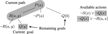
Figure 3: A state in the leanCoP solving process

To guide the proof search (Fig. 3), i.e. to select the next action, we use Monte Carlo Tree Search with policy and value, similar to the AlphaZero [42] algorithm. This means that the trainable model should take a leanCoP state as its input, and return estimated value of the state, i.e., the probability that the prover will win, and the action logits, i.e., real numbers assigned to every available action. The action probabilities are then computed from action logits using the softmax function.

To process the leanCoP state with our network, we first need to convert it to a list of clauses. If there are $A$ axioms, and a path of length $P$, we give the network the $A+P+1$ clauses: every axiom is a clause and every element in the path is a clause consisting of one literal. The last clause given to the network consists of all the unfinished goals, both under the current path and in earlier branches. This roughly corresponds to the set of clauses from which we aim to obtain the contradiction. The initial labels of the clauses can be therefore of 3 types: a clause originating from a goal, a member of a path, or an axiom. Each of these types represent a learnable initial vector of dimension 4.

The symbols can be of two types: predicates and functions, their initial value is represented by a single real number: zero for predicates, and a learnable number for functions. For term nodes, variables in different axioms are always considered to be different, and they are also considered to be different from the variables in the tableaux (note that unification performs variable renaming). Variables in the tableaux are shared among the path and the goals. Every term node can be of four types: a variable in an axiom, a variable in the tableaux, a literal, or another term. The term nodes have initial dimension 4.

Afterwards, we propagate through five message passing layers, with dimensions $d_{\mathbf{c}}^{i}=d_{\mathbf{c}}^{i}=32$, $d_{\mathbf{s}}^{i}=64$, obtaining $c_{5,j}$, $s_{5,j}$ and $t_{5,j}$. Then we consider all the $c_{5,j}$ vectors, apply a hidden layer of size 64 with ReLU activation to them, apply the $\mathop{\mathrm{red}}\limits$ reduction and use one more hidden layer of size 64 with ReLU activation. The final value is then computed by a linear layer with sigmoid activation.

Given the general setup, we now describe how we compute the logit for an action corresponding to the use of axiom $C_{i}$, and complementing its literal $T_{j}$ with the current goal. Let $C_{k}$ represents the clause of all the remaining goals. We concatenate $c_{5,i}$, $t_{5,j}$ and $c_{5,k}$, process it with a hidden layer of size 64 with ReLU activation, and then use a linear output layer (without the activation function).

With the leanCoP prover, we perform four solving and training iterations. In every solving iteration, we attempt to solve every problem in the dataset, generating training data in the meantime. The training data are then used for training the network, minimizing the cross-entropy with the target action probabilities and the MSE of the target value of every trained state. Every solving iteration therefore produces the target for action policy, and for value estimation, that are used for the following training.

The solving iteration number 0 (we also call it “bare prover”) is performed differently from the following ones. We use the prover without guidance, performing random steps with the step limit 200 repeatedly within a time limit. For every proof we find, we run the random solver again from every partial point in the proof, estimating the probabilities that the particular actions will lead to a solution. This is our training data for action probabilities. In order to get training data for value, we take all the states which we estimated during the computation of action probabilities. If the probability of finding a proof is non-zero in that state, we give it value 1, otherwise, we give it value 0.

Every other solving iteration is based on the network guidance in an MCTS setting, analogously to AlphaZero [42] and to the rlCoP system [26]. In order to decide on the action, we first built a game tree of size 200 according to the PUCT formula

$$U(s,a)=\log\left(\frac{1+N(s)+c_{\mathrm{base}}}{c_{\mathrm{base}}}\right)\cdot\frac{\sqrt{N(s)}}{1+N(s,a)},$$

where the prior probabilities and values are given by the network, and then we select the most visited node (performing a bigstep). This contrasts to the previous experiment with a simpler clasifier [26] where every decision node is given 2000 new expansions (in addition to the expansions already performed on the node). Additionally a limit of game steps of 200 has been added. The target probabilities of any state in every bigstep is proportional the number of visit counts of the appropriate actions in the tree search. The target value in these states is boolean depending on whether the proof was ultimately found or not.

5 DeepMath Experiments

DeepMath is a dataset developed for the first deep learning experiments with premise selection [2] on the Mizar40 problems [25]. Unlike other datasets such as HOLStep [21], DeepMath contains first-order formulas which makes it more suitable for our network. We used the dataset for two experiments – premise selection (Section 5.1) and recovering symbol names from the structure, i.e. symbol guessing (Section 5.2).

5.1 Premise Selection

DeepMath contains 32524 conjectures, and a balanced list of positive and negative premises for each conjecture. There are on average 8 positive and 8 negative premises for each conjecture. The task we consider first is to tell apart the positive and negative premises.

For our purposes, we randomly divided the conjectures into 3252 testing conjectures and 29272 training conjectures. For every conjecture, we clausified the negated conjecture together with all its (negative and positive) premises, and gave them all as input to the network (as a set of clauses). We kept the hyperparameters from the leanCoP experiment. There are two differences. First, there are just two types of clause nodes: negated conjectures and premises. Second, we consider just one type of variable nodes.

To obtain the output, we reduce (using the $\mathop{\mathrm{red}}\limits$ function introduced in Section 2) the clause nodes belonging to the conjecture and we do the same also for each premise. The the two results are concatenated and pushed through a hidden layer of size 128 with ReLU activation. Finally, an output layer (with sigmoid activation) is applied to obtain the estimated probability of the premise being positive (i.e., relevant for the conjecture).

5.2 Recovering Symbol Names from the Structure

In addition to the standard premise selection task, our setting is also suitable for defining and experimenting with a novel interesting task: guessing the names of the symbols from the structure of the formula. In particular, since the network has no information about the names of the symbols, it is interesting to see how much the trained system can correctly guess the exact names of the function and predicates symbols based just on the problem structure.

One of the interesting uses is for conjecturing by analogies [15], i.e., creating new conjectures by detecting and following alignments of various mathematical theories and concepts. Typical examples include the alignment between the theories of additive and multiplicative groups, complex and real vector spaces, dual operations such as join and meet in lattices, etc. The first systems used for alignment detection have been so far manually engineered [14], whereas in our setting such alignment is just a byproduct of the structural learning.

There are two ways how a new unique symbol can arise during the clausification process. Either as a Skolem function, or as a new definition (predicate) that represents parts of the original formulas. We performed two experiments based on how such new symbols are handled. We either ignore them, and train the neural network on the original (labeled) symbols only, or we give to all the new symbols the common labels skolem and def. Table 1 shows the frequencies of the five most common symbols in the DeepMath dataset after the clausification. Note that the newly introduced skolems and definitions account for almost 40% of the data.

TPTP name	def	skolem	=	m1_subset_1	k1_zfmisc_1
Mizar name	N/A	N/A	=	Element	bool
Frequency	21.5%	17.3%	2.0%	1.7%	1.2%

Table 1: The most common symbols in the clausified DeepMath.

6 Experimental Results

6.1 Guiding leanCoP

We evaluate our neural guided leanCoP against rlCoP [26]. Note however, that for both systems we use 200 playouts per MCTS decision so the rlCoP results presented here are different from [26]. We start with a set of leanCoP states with their values and action probabilities coming from the 4595 training problems solved with the bare random prover.

After training on this set, the MCTS guided by our network manages to solve 11978 training (160.7% more) and 1322 (159.2% more) testing problems, in total 13300 problems (160.5% more – Fig. 4). This is in total 49.1% more than rlCoP guided by XGBoost which in the same setup and with the same limits solves 8012 training problems, 908 testing problems, and 8920 problems in total. The improvement in the first iteration over XGBoost on the training and testing set is 49.5% and 45.6% respectively.

Subsequent iterations are also much better than for rlCoP, with slower progress already in third iteration (note that rlCoP also loses problems, starting with 6th iteration). The evaluation ran 100 provers in parallel on multiple CPUs communicating with the network running on a GPU. Receiving the queries from the prover takes on average 0.1 s, while the message-passing layers alone take around 0.12 s per batch. The current main speed issue turned out to be the communication overhead between the provers and the network. The average inference step in 100 agents and one network inference took on average 0.57 sec.

invariant net guided	bare	iter. 1	iter. 2	iter. 3
overall	5105	13300	14042	14002
training	4595	11978	12648	12642
testing	510	1322	1394	1360
rlCoP	bare	iter. 1	iter. 2	iter. 3
overall	5105	8920	10030	10959
training	4595	8012	9042	9874
testing	510	908	988	1085

Figure 4: Comparison of the number of problems solved by leanCoP guided by the invariant-preserving GNN and by XGBoost.

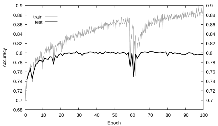
Figure 5: Testing and training accuracy on the premise selection task on the DeepMath dataset.

6.2 Premise Selection

In the first DeepMath experiment with Boolean classification, we obtained testing accuracy of around $80\%$. We trained the network in 100 epochs on minibatches of size 50. A stability issue can be spotted around the epoch 60 from which the network quickly recovered. We cannot compare the results to the standard methods since the dataset is by design hostile to them – the negatives samples are based on the KNN, so KNN has accuracy even less than $50\%$. Simpler neural networks were previously tested on the same dataset [29] reaching accuracy $76.45\%$ .

6.3 Recovering Symbol Names from the Structure

For guessing of symbol names, we used minibatches consisting only of 10 queries, and trained the network for 50 epochs. When training and evaluating on the labeled symbols only, the testing accuracy reached $65.27\%$ in the last epoch. Note that this accuracy is measured on the whole graph, i.e., we count both the symbols of the conjecture and of the premises. When training and evaluating also on the def and skolem symbols, the testing accuracy reached $78.4\%$ in the last epoch – see Fig. 7.

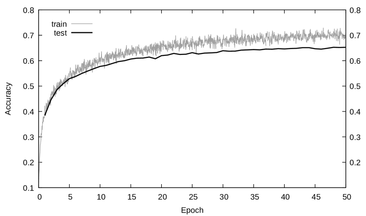
Figure 6: Testing and training accuracy on the label guessing task on the DeepMath dataset.

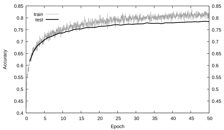
Figure 7: Testing and training accuracy on the label guessing task including labels def and skolem on the DeepMath dataset.

We evaluate the symbol guessing (without considering def and skolem) in more detail on the 3252 test problems and their conjectures. In particular, for each of these problems and each conjecture symbol, the evaluation with the trained network gives a list of candidate symbol names ranked by their probability. We first compute the number of cases where the most probable symbol name as suggested by the trained network is the correct one. This happens in 22409 cases out of 32196, i.e., in 70% cases. A perfect naming of all symbols is achieved for 544 conjectures, i.e., in 16.7% of the test cases. Some of the most common analogies measured as the common symbol-naming mistakes done on the test conjectures are shown in Table 2.

Table 2: Some of the common analogies

count	original Mizar symbol	Mizar analogy
129	Relation-like	Function-like
69	void	empty
53	Abelian	add-associative
47	total	-defined
45	0	1
40	+	*
39	reflexive	transitive
38	Function-like	FinSequence-like
33	-	+
31	trivial	empty
28	$>=$	=
27	associative	transitive
26	infinite	Function-like
25	empty	degenerated
24	real	natural
23	sigma-multiplicative	compl-closed
20	REAL	COMPLEX
18	transitive	reflexive
18	RelStr	TopStruct
18	Category-like	transitive
17	=	c=
16	initial	infinite
16	[Graph-like]	Function-like
16	associative	Group-like
16	0	{}
16	/	*
15	add-associative	associative
15	-	*
13	width	len
13	integer	natural
13	in	c=
12	$\cap$	$\cup$
11	c=	$>=$
10	with_infima	with_suprema
10	ordinal	natural
9	closed	open
8	sup	inf
8	Submodule	Subspace
7	Int	Cl

We briefly analyze some of the analogies produced by the network predictions. In theorem XBOOLE_1:25 below, the trained network’s best guess correctly labels the symbols as binary intersection and union (both with probability ca 0.75). Its second best guess is however also quite probable ($p=0.2$), swapping the union and intersection. This is quite common, probably because dual theorems about these two symbols are frequent in the training data. Interestingly, the second best guess results also in an provable conjecture, since it easily follows from XBOOLE_1:25 just by symmetry of equality.

⬇

theorem :: XBOOLE_1:25

for X, Y, Z being set holds ((X /\ Y) \/ (Y /\ Z)) \/ (Z /\ X) = ((X \/ Y) /\ (Y \/ Z)) /\ (Z \/ X)

second guess:

for X, Y, Z being set holds ((X \/ Y) /\ (Y \/ Z)) /\ (Z \/ X) = ((X /\ Y) \/ (Y /\ Z)) \/ (Z /\ X)

In theorem CLVECT_1:72 the trained network has consistently decided to replace the symbols defined for complex vector spaces with their analogs defined for real vector spaces (i.e., those symbols are ranked higher). This is most likely because of the large theory of real vector spaces in the training data, even though the exact theorem RLSUB_1:53 was not among the training data. This again means that the trained network has produced RLSUB_1:53 as a new (provable) conjecture.

⬇

theorem :: CLVECT_1:72

for V being ComplexLinearSpace for u, v being VECTOR of V

for W being Subspace of V holds

( u in W iff v + W = (v - u) + W )

theorem :: RLSUB_1:53

for V being RealLinearSpace for u, v being VECTOR of V

for W being Subspace of V holds

( u in W iff v + W = (v - u) + W )

Finally, we show below two examples. The first one illustrates on theorems LATTICE4:15 and LATTICE4:23 the network finding well-known dualities of concepts in lattices (join vs. meet, upper-bounded vs. lower-bounded and related concepts). The second one is an example of a discovered analogy between division and subtraction operations on complex numbers, i.e, conjecturing MEMBER_1:130 from MEMBER_1:77.

⬇

theorem :: LATTICE4:15

for 0L being lower-bounded Lattice

for B1, B2 being Finite_Subset of the carrier of 0L holds

(FinJoin B1) "\/" (FinJoin B2) = FinJoin (B1 \/ B2)

similar to:

theorem Th23: :: LATTICE4:23

for 1L being upper-bounded Lattice

for B1, B2 being Finite_Subset of the carrier of 1L holds

(FinMeet B1) "/\" (FinMeet B2) = FinMeet (B1 \/ B2)

theorem :: MEMBER_1:77

for a, b, s being complex number holds

{a,b} -- {s} = {(a - s),(b - s)}

similar to:

theorem :: MEMBER_1:130

for a, b, s being complex number holds

{a,b} /// {s} = {(a / s),(b / s)}

7 Related Work

Early work on combining machine learning with automated theorem proving includes, e.g., [10, 8, 40]. Machine learning over large formal corpora created from ITP libraries [45, 34, 22] has been used for premise selection [44, 47, 30, 2], resulting in strong hammer systems for selecting relevant facts for proving new conjectures over large formal libraries [1, 4, 12]. More recently, machine learning has also started to be used to guide the internal search of the ATP systems. In saturation-style provers this has been done by feedback loops for strategy invention [46, 18, 39] and by using supervised learning [19, 33] to select the next given clause [37]. In the simpler connection tableau systems such as leanCoP [36] used here, supervised learning has been used to choose the next tableau extension step [48, 23], using Monte-Carlo guided proof search [11] and reinforcement learning [26] with fast non-deep learners. Our main evaluation is done in this setting.

Deep neural networks for classification of mathematical formulae were first introduced in the DeepMath experiments [2] with 1D convolutional networks and LSTM networks. For higher-order logic, the HolStep [21] dataset was extracted from interactive theorem prover HOL Light. 1D convolutional neural networks, LSTM, and their combination were proposed as baselines for the dataset. On this dataset a Graph-based neural network was for a first time applied to theorem proving in the FormulaNet [49] work. FormulaNet, like our work, also represents identical variables by a single nodes in a graph, being therefore invariant under variable renaming. Unlike our network, FormulaNet glues variables only and not more complex terms. FormulaNet is not designed specifically for first-order logic, therefore it lacks invariance under negation and possibly reordering of clauses and literals. The greatest difference is however that our network abstracts over the symbol names while FormulaNet learns them individually.

A different invariance property was proposed in a network for propositional calculus by Selsam et al. [41]. This network is invariant under negation, order of clauses, and order of literals in clauses, however this is restricted to propositional logic, where no quantifiers and variables are present. In the first-order setting, Kucik and Korovin [29] performed experiments with basic neural networks with one hidden layer on the DeepMath dataset. Neural networks reappeared in state-of-the-art saturation-based proving (E prover) in the work of Loos et al. [32]. The considered models included CNNs, LSTMs, dilated convolutions, and tree models. The first practical comparison of neural networks, XGBoost and Liblinear in guiding E prover was done by Chvalovsky et al. [6].

An alternative to connecting an identifier with all the formulas about it, is to perform definitional embeddings. This has for the first time been done in the context of theorem proving in DeepMath [2], however in a non-recursive way. A fully recursive, but non-deep name-independent encoding has been used and evaluated in HOLyHammer experiments [24]. Similarity between concepts has been discovered using alignments, see e.g. [13]. Embeddings of particular individual logical concepts have been considered as well, for example polynomials [3] or equations [28].

8 Conclusion

We presented a neural network for processing mathematical formulae invariant under symbol names, negation and ordering of clauses and their literals, and we demonstrated its learning capabilities in three automated reasoning tasks. In particular, the network improves over the previous version of rlCoP guided by XGBoost by 45.6% on the test set in the first iteration of learning-guided proving. It also outperforms earlier methods on the premise-selection data, and establishes a strong baseline for symbol guessing. One of its novel uses proposed here and allowed by this neural architecture is creating new conjectures by detecting and following alignments of various mathematical theories and concepts. This task turns out to be a straightforward application of the structural learning performed by the network.

Possible future work includes for example integration with state-of-the-art saturation-style provers. An interesting next step is also evaluation on a heterogeneous dataset such as TPTP where symbols are not used consistently and learning on multiple libraries – e.g. jointly on HOL and HOL Light as done previously by [13] using a hand-crafted alignment system.

9 Acknowledgements

Olšák and Kaliszyk were supported by the ERC Project SMART Starting Grant no. 714034. Urban was supported by the AI4REASON ERC Consolidator grant number 649043, and by the Czech project AI&Reasoning CZ.02.1.01/0.0/0.0/15_003/0000466 and the European Regional Development Fund.

References

- [1] Jesse Alama, Tom Heskes, Daniel Kühlwein, Evgeni Tsivtsivadze, and Josef Urban, ‘Premise selection for mathematics by corpus analysis and kernel methods’, J. Autom. Reasoning, 52(2), 191–213, (2014).
- [2] Alexander A. Alemi, François Chollet, Niklas Eén, Geoffrey Irving, Christian Szegedy, and Josef Urban, ‘DeepMath - deep sequence models for premise selection’, in Advances in Neural Information Processing Systems 29: Annual Conference on Neural Information Processing Systems 2016, December 5-10, 2016, Barcelona, Spain, eds., Daniel D. Lee, Masashi Sugiyama, Ulrike V. Luxburg, Isabelle Guyon, and Roman Garnett, pp. 2235–2243, (2016).
- [3] Miltiadis Allamanis, Pankajan Chanthirasegaran, Pushmeet Kohli, and Charles A. Sutton, ‘Learning continuous semantic representations of symbolic expressions’, in Proceedings of the 34th International Conference on Machine Learning, ICML 2017, Sydney, NSW, Australia, 6-11 August 2017, eds., Doina Precup and Yee Whye Teh, volume 70 of Proceedings of Machine Learning Research, pp. 80–88. PMLR, (2017).
- [4] Jasmin Christian Blanchette, David Greenaway, Cezary Kaliszyk, Daniel Kühlwein, and Josef Urban, ‘A learning-based fact selector for Isabelle/HOL’, J. Autom. Reasoning, 57(3), 219–244, (2016).
- [5] Jasmin Christian Blanchette, Cezary Kaliszyk, Lawrence C. Paulson, and Josef Urban, ‘Hammering towards QED’, J. Formalized Reasoning, 9(1), 101–148, (2016).
- [6] Karel Chvalovský, Jan Jakubuv, Martin Suda, and Josef Urban, ‘ENIGMA-NG: efficient neural and gradient-boosted inference guidance for E’, in Automated Deduction - CADE 27 - 27th International Conference on Automated Deduction, Natal, Brazil, August 27-30, 2019, Proceedings, ed., Pascal Fontaine, volume 11716 of Lecture Notes in Computer Science, pp. 197–215. Springer, (2019).
- [7] Martin Davis, Ansgar Fehnker, Annabelle McIver, and Andrei Voronkov, eds. Logic for Programming, Artificial Intelligence, and Reasoning - 20th International Conference, LPAR-20 2015, Suva, Fiji, November 24-28, 2015, Proceedings, volume 9450 of Lecture Notes in Computer Science. Springer, 2015.
- [8] Jörg Denzinger, Matthias Fuchs, Christoph Goller, and Stephan Schulz, ‘Learning from Previous Proof Experience’, Technical Report AR99-4, Institut für Informatik, Technische Universität München, (1999).
- [9] David Duvenaud, Dougal Maclaurin, Jorge Aguilera-Iparraguirre, Rafael Gómez-Bombarelli, Timothy Hirzel, Alán Aspuru-Guzik, and Ryan P. Adams, ‘Convolutional networks on graphs for learning molecular fingerprints’, in Advances in Neural Information Processing Systems 28: Annual Conference on Neural Information Processing Systems 2015, December 7-12, 2015, Montreal, Quebec, Canada, eds., Corinna Cortes, Neil D. Lawrence, Daniel D. Lee, Masashi Sugiyama, and Roman Garnett, pp. 2224–2232, (2015).
- [10] Wolfgang Ertel, Johann Schumann, and Christian B. Suttner, ‘Learning heuristics for a theorem prover using back propagation’, in 5. Österreichische Artificial Intelligence-Tagung, Igls, Tirol, 28. bis 30. September 1989, Proceedings, eds., Johannes Retti and Karl Leidlmair, volume 208 of Informatik-Fachberichte, pp. 87–95. Springer, (1989).
- [11] Michael Färber, Cezary Kaliszyk, and Josef Urban, ‘Monte Carlo tableau proof search’, in Automated Deduction - CADE 26 - 26th International Conference on Automated Deduction, Gothenburg, Sweden, August 6-11, 2017, Proceedings, ed., Leonardo de Moura, volume 10395 of Lecture Notes in Computer Science, pp. 563–579. Springer, (2017).
- [12] Thibault Gauthier and Cezary Kaliszyk, ‘Premise selection and external provers for HOL4’, in Certified Programs and Proofs (CPP’15), LNCS. Springer, (2015). http://dx.doi.org/10.1145/2676724.2693173.
- [13] Thibault Gauthier and Cezary Kaliszyk, ‘Sharing HOL4 and HOL light proof knowledge’, In Davis et al. [7], pp. 372–386.
- [14] Thibault Gauthier and Cezary Kaliszyk, ‘Aligning concepts across proof assistant libraries’, J. Symb. Comput., 90, 89–123, (2019).
- [15] Thibault Gauthier, Cezary Kaliszyk, and Josef Urban, ‘Initial experiments with statistical conjecturing over large formal corpora’, in Joint Proceedings of the FM4M, MathUI, and ThEdu Workshops, Doctoral Program, and Work in Progress at the Conference on Intelligent Computer Mathematics 2016 co-located with the 9th Conference on Intelligent Computer Mathematics (CICM 2016), Bialystok, Poland, July 25-29, 2016, eds., Andrea Kohlhase, Paul Libbrecht, Bruce R. Miller, Adam Naumowicz, Walther Neuper, Pedro Quaresma, Frank Wm. Tompa, and Martin Suda, volume 1785 of CEUR Workshop Proceedings, pp. 219–228. CEUR-WS.org, (2016).
- [16] Christoph Goller and Andreas Küchler, ‘Learning task-dependent distributed representations by backpropagation through structure’, in Proceedings of International Conference on Neural Networks (ICNN’96), Washington, DC, USA, June 3-6, 1996, pp. 347–352. IEEE, (1996).
- [17] Georg Gottlob, Geoff Sutcliffe, and Andrei Voronkov, eds. Global Conference on Artificial Intelligence, GCAI 2015, Tbilisi, Georgia, October 16-19, 2015, volume 36 of EPiC Series in Computing. EasyChair, 2015.
- [18] Jan Jakubův and Josef Urban, ‘Hierarchical invention of theorem proving strategies’, AI Commun., 31(3), 237–250, (2018).
- [19] Jan Jakubuv and Josef Urban, ‘ENIGMA: efficient learning-based inference guiding machine’, in Intelligent Computer Mathematics - 10th International Conference, CICM 2017, Edinburgh, UK, July 17-21, 2017, Proceedings, eds., Herman Geuvers, Matthew England, Osman Hasan, Florian Rabe, and Olaf Teschke, volume 10383 of Lecture Notes in Computer Science, pp. 292–302. Springer, (2017).
- [20] Jan Jakubuv and Josef Urban, ‘Hammering Mizar by learning clause guidance’, in 10th International Conference on Interactive Theorem Proving, ITP 2019, September 9-12, 2019, Portland, OR, USA, eds., John Harrison, John O’Leary, and Andrew Tolmach, volume 141 of LIPIcs, pp. 34:1–34:8. Schloss Dagstuhl - Leibniz-Zentrum für Informatik, (2019).
- [21] Cezary Kaliszyk, François Chollet, and Christian Szegedy, ‘HolStep: A machine learning dataset for higher-order logic theorem proving’, in 5th International Conference on Learning Representations, ICLR 2017, Toulon, France, April 24-26, 2017, Conference Track Proceedings. OpenReview.net, (2017).
- [22] Cezary Kaliszyk and Josef Urban, ‘Learning-assisted automated reasoning with Flyspeck’, J. Autom. Reasoning, 53(2), 173–213, (2014).
- [23] Cezary Kaliszyk and Josef Urban, ‘FEMaLeCoP: Fairly efficient machine learning connection prover’, In Davis et al. [7], pp. 88–96.
- [24] Cezary Kaliszyk and Josef Urban, ‘HOL(y)Hammer: Online ATP service for HOL Light’, Mathematics in Computer Science, 9(1), 5–22, (2015).
- [25] Cezary Kaliszyk and Josef Urban, ‘MizAR 40 for Mizar 40’, J. Autom. Reasoning, 55(3), 245–256, (2015).
- [26] Cezary Kaliszyk, Josef Urban, Henryk Michalewski, and Miroslav Olšák, ‘Reinforcement learning of theorem proving’, in Advances in Neural Information Processing Systems 31: Annual Conference on Neural Information Processing Systems 2018, NeurIPS 2018, 3-8 December 2018, Montréal, Canada., pp. 8836–8847, (2018).
- [27] Cezary Kaliszyk, Josef Urban, and Jirí Vyskocil, ‘Efficient semantic features for automated reasoning over large theories’, in IJCAI, pp. 3084–3090. AAAI Press, (2015).
- [28] Kriste Krstovski and David M. Blei, ‘Equation embeddings’, CoRR, abs/1803.09123, (2018).
- [29] Andrzej Stanislaw Kucik and Konstantin Korovin, ‘Premise selection with neural networks and distributed representation of features’, CoRR, abs/1807.10268, (2018).
- [30] Daniel Kühlwein, Twan van Laarhoven, Evgeni Tsivtsivadze, Josef Urban, and Tom Heskes, ‘Overview and evaluation of premise selection techniques for large theory mathematics’, in IJCAR, eds., Bernhard Gramlich, Dale Miller, and Uli Sattler, volume 7364 of LNCS, pp. 378–392. Springer, (2012).
- [31] Reinhold Letz, Klaus Mayr, and Christoph Goller, ‘Controlled integration of the cut rule into connection tableau calculi’, Journal of Automated Reasoning, 13, 297–337, (1994).
- [32] Sarah Loos, Geoffrey Irving, Christian Szegedy, and Cezary Kaliszyk, ‘Deep network guided proof search’, in LPAR-21. 21st International Conference on Logic for Programming, Artificial Intelligence and Reasoning, eds., Thomas Eiter and David Sands, volume 46 of EPiC Series in Computing, pp. 85–105. EasyChair, (2017).
- [33] Sarah M. Loos, Geoffrey Irving, Christian Szegedy, and Cezary Kaliszyk, ‘Deep network guided proof search’, in LPAR-21, 21st International Conference on Logic for Programming, Artificial Intelligence and Reasoning, Maun, Botswana, May 7-12, 2017, eds., Thomas Eiter and David Sands, volume 46 of EPiC Series in Computing, pp. 85–105. EasyChair, (2017).
- [34] Jia Meng and Lawrence C. Paulson, ‘Translating higher-order clauses to first-order clauses’, J. Autom. Reasoning, 40(1), 35–60, (2008).
- [35] Jens Otten, ‘Restricting backtracking in connection calculi’, AI Commun., 23(2-3), 159–182, (2010).
- [36] Jens Otten and Wolfgang Bibel, ‘leanCoP: lean connection-based theorem proving’, J. Symb. Comput., 36(1-2), 139–161, (2003).
- [37] Ross A. Overbeek, ‘A new class of automated theorem-proving algorithms’, J. ACM, 21(2), 191–200, (April 1974).
- [38] Handbook of Automated Reasoning (in 2 volumes), eds., John Alan Robinson and Andrei Voronkov, Elsevier and MIT Press, 2001.
- [39] Simon Schäfer and Stephan Schulz, ‘Breeding theorem proving heuristics with genetic algorithms’, In Gottlob et al. [17], pp. 263–274.
- [40] Stephan Schulz, Learning search control knowledge for equational deduction, volume 230 of DISKI, Infix Akademische Verlagsgesellschaft, 2000.
- [41] Daniel Selsam, Matthew Lamm, Benedikt Bünz, Percy Liang, Leonardo de Moura, and David L. Dill, ‘Learning a SAT solver from single-bit supervision’, in 7th International Conference on Learning Representations, ICLR 2019, New Orleans, LA, USA, May 6-9, 2019. OpenReview.net, (2019).
- [42] David Silver, Julian Schrittwieser, Karen Simonyan, Ioannis Antonoglou, Aja Huang, Arthur Guez, Thomas Hubert, Lucas Baker, Matthew Lai, Adrian Bolton, et al., ‘Mastering the game of go without human knowledge’, Nature, 550(7676), 354, (2017).
- [43] Geoff Sutcliffe, ‘The TPTP world - infrastructure for automated reasoning’, in LPAR (Dakar), eds., Edmund M. Clarke and Andrei Voronkov, volume 6355 of LNCS, pp. 1–12. Springer, (2010).
- [44] Josef Urban, ‘MPTP - Motivation, Implementation, First Experiments’, J. Autom. Reasoning, 33(3-4), 319–339, (2004).
- [45] Josef Urban, ‘MPTP 0.2: Design, implementation, and initial experiments’, J. Autom. Reasoning, 37(1-2), 21–43, (2006).
- [46] Josef Urban, ‘BliStr: The Blind Strategymaker’, In Gottlob et al. [17], pp. 312–319.
- [47] Josef Urban, Geoff Sutcliffe, Petr Pudlák, and Jiří Vyskočil, ‘MaLARea SG1 - Machine Learner for Automated Reasoning with Semantic Guidance’, in IJCAR, eds., Alessandro Armando, Peter Baumgartner, and Gilles Dowek, volume 5195 of LNCS, pp. 441–456. Springer, (2008).
- [48] Josef Urban, Jiří Vyskočil, and Petr Štěpánek, ‘MaLeCoP: Machine learning connection prover’, in TABLEAUX, eds., Kai Brünnler and George Metcalfe, volume 6793 of LNCS, pp. 263–277. Springer, (2011).
- [49] Mingzhe Wang, Yihe Tang, Jian Wang, and Jia Deng, ‘Premise selection for theorem proving by deep graph embedding’, in Advances in Neural Information Processing Systems 30: Annual Conference on Neural Information Processing Systems 2017, 4-9 December 2017, Long Beach, CA, USA, eds., Isabelle Guyon, Ulrike von Luxburg, Samy Bengio, Hanna M. Wallach, Rob Fergus, S. V. N. Vishwanathan, and Roman Garnett, pp. 2786–2796, (2017).