The partonic structure of the electron at the next-to-leading logarithmic accuracy in QED

Abstract

By working in QED, we obtain the electron, positron, and photon Parton Distribution Functions (PDFs) of the unpolarised electron at the next-to-leading logarithmic accuracy. The PDFs account for all of the universal effects of initial-state collinear origin, and are key ingredients in the calculations of cross sections in the so-called structure-function approach. We present both numerical and analytical results, and show that they agree extremely well with each other. The analytical predictions are defined by means of an additive formula that matches a large-$z$ solution that includes all orders in the QED coupling constant $\alpha$, with a small- and intermediate-$z$ solution that includes terms up to ${\cal O}(\alpha^{3})$.

1 Introduction

The typical cross section relevant to $e^{+}e^{-}$ collisions is in principle entirely computable as a perturbative series in the QED coupling constant $\alpha$. In practice, however, this is hardly useful, since the coefficients of such a series are very large, thus compensating the suppression due to $\alpha$ – in other words, all terms of the series might be of the same order numerically, which leads to a complete loss of predictive power. The problem stems from the fact that the incoming $e^{\pm}$ particles tend to copiously radiate photons (which in turn may convert into $e^{+}e^{-}$ pairs, and so forth) at small angles w.r.t. the beamline. In perturbation theory, any zero-angle emission would induce a divergent cross section, were it not for the screening effect provided by the mass of the emitter and/or the emitted particle. Thus, when integrating over all possible emissions, the cross section will contain logarithms of the ratio $m^{2}/E^{2}$, where $E$ is a scale of the order of the hardness of the process, and $m$ is the screening mass (i.e. that of the electron in the case we are interested in). It is these logarithms that, by growing large when $m^{2}/E^{2}\ll 1$, give the dominant contributions to the perturbative coefficients, and ultimately prevent the series from being well behaved.

Fortunately, such $\log(m^{2}/E^{2})$ terms are universal, and because of this they can be taken into account to all orders in $\alpha$ by a process-independent resummation procedure. In the so-called structure-function approach, the physical cross section is then written by means of a factorisation formula such as the following one:

$$d\bar{\sigma}_{e^{+}e^{-}}(p_{e^{+}},p_{e^{-}},m^{2}) = \sum_{ij=e^{\pm},\gamma}\int dz_{+}dz_{-}\,\Gamma_{\!i/e^{+}}(z_{+},\mu^{2},m^{2})\,\Gamma_{\!j/e^{-}}(z_{-},\mu^{2},m^{2})$$ (1)

$$\phantom{\sum_{ij}\int}\times d\hat{\sigma}_{ij}(z_{+}p_{e^{+}},z_{-}p_{e^{-}},\mu^{2})\,.$$

The quantities $\Gamma_{\!i/e^{\pm}}$ are called the Parton Distribution Functions (PDFs) of the electron or the positron, a name that originates from the analogy of eq. (1) with its QCD counterpart. PDFs collect and resum all of the $\log(m^{2}/E^{2})$ terms; conversely, the short-distance cross sections $d\hat{\sigma}_{ij}$ do not contain any such logarithms, and are expected to be well-behaved order by order in perturbation theory. Neither $\Gamma_{\!i/e^{\pm}}$ nor $d\hat{\sigma}_{ij}$ are physical quantities; their definitions always involve some degree of arbitrariness, which is parametrised by the mass scale $\mu$, that is only constrained by the requirement $\mu\sim E$, and by the chosen factorisation scheme.

Fuller details on the usage of the factorisation formula (1) in calculations relevant to $e^{+}e^{-}$ colliders and on its physical meaning can be found e.g. in ref. Frixione:2019lga . In particular, we shall adopt the notation of ref. Frixione:2019lga , whereby the incoming $e^{\pm}$ are called particles (with $d\bar{\sigma}_{e^{+}e^{-}}$ thus being a particle-level cross section, defined so as to retain only terms that do not vanish in the $m/E\to 0$ limit), and the objects $i$ and $j$ are called partons (so that $d\hat{\sigma}_{ij}$ is a parton-level cross section). This allows one to distinguish easily between an electron that stems from one of the collider beams, and an electron that initiates the hard collisions, and that stems from the PDF $\Gamma_{\!e^{-}/e^{-}}$.

We point out that it is somehow customary in QED to call $\Gamma_{\!e^{-}/e^{-}}$ ($\Gamma_{\!e^{+}/e^{+}}$) the electron (positron) structure function. This is motivated by the fact that, by ignoring the contributions of partons whose species is not the same as that of the incoming particle, and by working at the first order in perturbation theory, a structure function (which is an observable) can be made to coincide with the PDF relevant to the case where particle and parton have the same identity, by means of a suitable definition of such a PDF. This position is not tenable at higher perturbative orders, and when more parton species are allowed in any given particle. Therefore, “structure functions” will not be used in this paper, and we shall only refer to PDFs.

The crucial point that we need to stress here is that in QED $e^{\pm}$ PDFs, at variance with hadronic PDFs, are entirely calculable with perturbative techniques. Presently they are known in close analytical forms Skrzypek:1990qs ; Skrzypek:1992vk ; Cacciari:1992pz which are leading-logarithmic (LL) accurate, and that include all-order in $\alpha$ contributions in the region $z_{\pm}\simeq 1$ (which is responsible for the bulk of the cross section), matched with up to ${\cal O}(\alpha^{3})$ terms for any values of $z_{\pm}$; both of these forms exploit leading-order (LO) initial conditions. The goal of the present work is to improve on the results of refs. Skrzypek:1990qs ; Skrzypek:1992vk ; Cacciari:1992pz by extending them to the next-to-leading logarithm accuracy (NLL) starting from the next-to-leading order (NLO) initial conditions computed in ref. Frixione:2019lga . In keeping with what was done in the literature, we shall present predictions both for all-order PDFs in the $z_{\pm}\simeq 1$ region, and for up to ${\cal O}(\alpha^{3})$ NLL terms valid for any $z_{\pm}$. By working at the NLL+NLO accuracy, the mixing between the electron/positron and the photon PDFs is taken into proper account, as are running-$\alpha$ effects. Our results are obtained with both analytical and numerical methods, which are compared and used to validate each other.

This paper is organised as follows. For those readers who are not interested in the technical procedures which underpin this work but only in their final outcomes, we summarise our final results in sect. 2. The details of the derivations of such results are then given in the remainder of the paper. In sect. 3 we introduce the evolution equations for the PDFs that we are going to solve, and report the associated initial conditions. Sect. 4 briefly describes the evolution-operator formalism. Analytical solutions are computed in sect. 5, for any $z_{\pm}$ values in sect. 5.1 (the resulting lengthy expressions are partly collected in appendix A), and for $z_{\pm}\simeq 1$ in sect. 5.2 (with additional details reported in appendix B), while a description of the codes employed to obtain numerical results is given in sect. 6. The solutions of sects. 5.1 and 5.2 are combined (“matched”) in sect. 7. Our analytical and numerical predictions are extensively compared in sect. 8. Finally, we conclude and give a short outlook in sect. 9. Additional material is collected in the appendices.

2 Synopsis of results

The $e^{\pm}$ PDFs that we shall compute in this paper result from solving the evolution equations of eqs. (12)–(13), with the initial conditions given in eqs. (25)–(28). The all-order, large-$z$ solutions and one of the numerical codes we shall employ require the use of an evolution operator, whose RGE is presented in eq. (44). The latter can be solved in a closed form in the case of a one-dimensional flavour space; such a closed form is reported either in eq. (46) or in eq. (50), the two differing by terms of ${\cal O}(\alpha^{3})$ and with the latter form suitable to take the fixed-$\alpha$ limit. The two-dimensional flavour space case is discussed in appendix B. The PDF solutions valid for any $z$ and including up to ${\cal O}(\alpha^{3})$ contributions are represented in terms of sets of basis functions, which are obtained by solving recursive equations; these are given in eqs. (80) and (5.1), and their explicit solutions partly in appendix A, and partly in an ancillary file (see below). Conversely, the all-order, large-$z$ solutions for the PDFs are reported in eq. (96) (LL accurate for singlet and non-singlet), eq. (357) (LL accurate for photon), eq. (113) (NLL accurate with running $\alpha$ for singlet and non-singlet), eq. (343) (NLL accurate with running $\alpha$ for photon), and eq. (118) (NLL accurate with fixed $\alpha$ for singlet and non-singlet; the corresponding result for the photon is obtained from eq. (343), but is not reported explicitly). The all-$z$ and large-$z$ solutions are then matched in an additive manner, as is shown in eq. (131). The arXiv submission of the present work will be accompanied by two ancillary files, that will contain the main results for the PDFs as Mathematica formulae, and some analytical results too long to fit in this paper. Furthermore, a numerical code that returns the PDFs will be made public, to be downloaded at:

                           https://github.com/gstagnit/ePDF.

3 Evolution equations and initial conditions

By working in QED the cases of the electron and of the positron PDFs are identical. Thus, in order to be definite in this paper we shall only consider the PDFs of the electron, which allows us to simplify the notation of ref. Frixione:2019lga in the following way:

$$\Gamma_{\!i}(z,\mu^{2})\big{[}{\rm this~{}paper}\big{]}\;\equiv\;\Gamma_{\!i/e^{-}}(z,\mu^{2})\big{[}{\rm ref}.~{}\text{\cite[cite]{\@@bibref{Authors Phrase1YearPhrase2}{Frixione:2019lga}{\@@citephrase{(}}{\@@citephrase{)}}}}\big{]}\,.$$ (2)

The evolution equations are therefore Gribov:1972ri ; Lipatov:1974qm ; Altarelli:1977zs ; Dokshitzer:1977sg :

$$\frac{\partial\Gamma_{\!i}(z,\mu^{2})}{\partial\log\mu^{2}}=\frac{\alpha(\mu)}{2\pi}\left[P_{ij}\otimes\Gamma_{\!j}\right](z,\mu^{2})\,.$$ (3)

Henceforth, we shall omit to write the explicit $z$ and/or $\mu$ dependences when no confusion can possibly arise. By working with a single fermion family, eq. (3) becomes:

$$\frac{\partial\Gamma_{\!e^{-}}}{\partial\log\mu^{2}} = \frac{\alpha}{2\pi}\Big{(}P_{e^{-}e^{-}}\otimes\Gamma_{\!e^{-}}+P_{e^{-}e^{+}}\otimes\Gamma_{\!e^{+}}+P_{e^{-}\gamma}\otimes\Gamma_{\!\gamma}\Big{)}\,,$$ (4)

$$\frac{\partial\Gamma_{\!e^{+}}}{\partial\log\mu^{2}} = \frac{\alpha}{2\pi}\Big{(}P_{e^{+}e^{-}}\otimes\Gamma_{\!e^{-}}+P_{e^{+}e^{+}}\otimes\Gamma_{\!e^{+}}+P_{e^{+}\gamma}\otimes\Gamma_{\!\gamma}\Big{)}\,,$$ (5)

$$\frac{\partial\Gamma_{\!\gamma}}{\partial\log\mu^{2}} = \frac{\alpha}{2\pi}\Big{(}P_{\gamma e^{-}}\otimes\Gamma_{\!e^{-}}+P_{\gamma e^{+}}\otimes\Gamma_{\!e^{+}}+P_{\gamma\gamma}\otimes\Gamma_{\!\gamma}\Big{)}\,.$$ (6)

This system of equations can be simplified by introducing the singlet and non-singlet combinations:

$$\Gamma_{\!\rm\scriptscriptstyle S}=\Gamma_{\!e^{-}}+\Gamma_{\!e^{+}}\,,\;\;\;\;\;\;\;\;\Gamma_{\!\rm\scriptscriptstyle NS}=\Gamma_{\!e^{-}}-\Gamma_{\!e^{+}}\,.$$ (7)

Equations (4)–(6) are then re-written as follows:

$$\frac{\partial}{\partial\log\mu^{2}}\left(\!\!\begin{array}[]{c}\Gamma_{\!\rm\scriptscriptstyle S}\\ \Gamma_{\!\gamma}\end{array}\!\!\right) = \frac{\alpha}{2\pi}{\mathbb{P}}_{\rm\scriptscriptstyle S}\otimes\left(\!\!\begin{array}[]{c}\Gamma_{\!\rm\scriptscriptstyle S}\\ \Gamma_{\!\gamma}\end{array}\!\!\right)\,,$$ (12)

$$\frac{\partial\Gamma_{\!\rm\scriptscriptstyle NS}}{\partial\log\mu^{2}} = \frac{\alpha}{2\pi}P_{\rm\scriptscriptstyle NS}\otimes\Gamma_{\!\rm\scriptscriptstyle NS}\,,$$ (13)

which show, as is customary, that the non-singlet component decouples (i.e. evolves independently) from the singlet-photon system. The evolution kernels in eqs. (12) and (13) are defined by starting from the elementary Altarelli-Parisi kernels. One uses the following decomposition:

$$P_{e^{\pm}e^{\pm}}=P^{\rm\scriptscriptstyle V}_{ee}+P^{\rm\scriptscriptstyle S}_{ee}\,,\;\;\;\;\;\;\;\;P_{e^{\pm}e^{\mp}}=P^{\rm\scriptscriptstyle V}_{e\bar{e}}+P^{\rm\scriptscriptstyle S}_{ee}\,.$$ (14)

Furthermore, in QED:

$$P_{e^{\pm}\gamma}=P_{e\gamma}\,,\;\;\;\;\;\;\;\;\phantom{+P^{\rm\scriptscriptstyle S}_{ee}}\;\;\;P_{\gamma e^{\pm}}=P_{\gamma e}\,.$$ (15)

Thus, by introducing the quantities:

$$P_{\Sigma\Sigma} = P_{e^{\pm}e^{\pm}}+P_{e^{\pm}e^{\mp}}\equiv P^{\rm\scriptscriptstyle V}_{ee}+P^{\rm\scriptscriptstyle V}_{e\bar{e}}+2n_{\scriptscriptstyle F}P^{\rm\scriptscriptstyle S}_{ee}\,,\;\;\;\;\;\;\;\;n_{\scriptscriptstyle F}=1\,,$$ (16)

$$P_{\Sigma\gamma} = 2n_{\scriptscriptstyle F}P_{e\gamma}\,,$$ (17)

$$P_{\gamma\Sigma} = P_{\gamma e}\,,$$ (18)

one finally defines the evolution kernels:

$${\mathbb{P}}_{\rm\scriptscriptstyle S} = \left(\begin{array}[]{cc}P_{\Sigma\Sigma}&P_{\Sigma\gamma}\\ P_{\gamma\Sigma}&P_{\gamma\gamma}\\ \end{array}\right)\,,$$ (21)

$$P_{\rm\scriptscriptstyle NS} = P_{e^{\pm}e^{\pm}}-P_{e^{\pm}e^{\mp}}\equiv P^{\rm\scriptscriptstyle V}_{ee}-P^{\rm\scriptscriptstyle V}_{e\bar{e}}\,.$$ (22)

After solving the evolution equations for the singlet and non-singlet components, one recovers the solutions for the electron and the positron by inverting eq. (7):

$$\Gamma_{\!e^{-}}=\frac{1}{2}\left(\Gamma_{\!\rm\scriptscriptstyle S}+\Gamma_{\!\rm\scriptscriptstyle NS}\right)\,,\;\;\;\;\;\;\;\;\Gamma_{\!e^{+}}=\frac{1}{2}\left(\Gamma_{\!\rm\scriptscriptstyle S}-\Gamma_{\!\rm\scriptscriptstyle NS}\right)\,.$$ (23)

The electron PDFs can be expanded perturbatively. We denote the first two coefficients of such an expansion in the same way as in ref. Frixione:2019lga , namely:

$$\Gamma_{\!i}=\Gamma_{\!i}^{[0]}+\frac{\alpha}{2\pi}\,\Gamma_{\!i}^{[1]}+{\cal O}(\alpha^{2})\,.$$ (24)

The evolution equations are supplemented by the initial conditions computed up to ${\cal O}(\alpha)$ in ref. Frixione:2019lga . These read as follows:

$$\Gamma_{\!i}^{[0]}(z,\mu_{0}^{2}) = \delta_{ie^{-}}\delta(1-z)\,,$$ (25)

$$\Gamma_{\!e^{-}}^{[1]}(z,\mu_{0}^{2}) = \left[\frac{1+z^{2}}{1-z}\left(\log\frac{\mu_{0}^{2}}{m^{2}}-2\log(1-z)-1\right)\right]_{+}+K_{ee}(z)\,,$$ (26)

$$\Gamma_{\!\gamma}^{[1]}(z,\mu_{0}^{2}) = \frac{1+(1-z)^{2}}{z}\left(\log\frac{\mu_{0}^{2}}{m^{2}}-2\log z-1\right)+K_{\gamma e}(z)\,,$$ (27)

$$\Gamma_{\!e^{+}}^{[1]}(z,\mu_{0}^{2}) = 0\,,$$ (28)

where $\mu_{0}\simeq m$, and $m$ is the electron mass. The rightmost terms on the r.h.s. of eqs. (26) and (27) are associated with, and fully determined by, the scheme used to subtract the initial-state collinear singularities. In this paper, we work in the $\overline{\rm MS}$ scheme, which implies:

$$K_{ee}(z)=K_{\gamma e}(z)=0\;\;\;\;\Longleftrightarrow\;\;\;\;\overline{\rm MS}\,.$$ (29)

We conclude this section with a general remark on evolution. Throughout this paper, by “evolution” we understand the one governed by RGE’s. This implies, in particular, that the contributions of $e^{+}e^{-}$ low-energy data to the running of $\alpha$ are locally neglected (i.e. for scales of the order of the masses of light hadronic resonances). However, nothing prevents one from taking into account such contributions in an inclusive way. Namely, by starting from a precise determination of $\alpha=\alpha_{H}$ that does include low-energy contributions, and that can be associated with a scale $\mu_{H}$ (just) larger than the mass of the heaviest hadronic resonance, one can backward-evolve $\alpha_{H}=\alpha(\mu_{H})$ from $\mu_{H}$ down to $\mu_{0}$, thus determining the value of $\alpha(\mu_{0})$ that is employed in this work. By doing so, the possible local effects of the resonances on the evolution of the PDFs are still neglected, but this is not important: in the factorisation formulae such as eq. (1) where the PDFs are used, the scales are meant to be hard and therefore never assume values comparable to the masses of the light hadronic resonances.

4 Evolution operator

As far as the evolution in $\mu$ is concerned, eqs. (12) and (13) are identical. We shall thus start dealing with the former one, which has a more involved flavour structure; the results will then be applied to the non-singlet case as well, by simply considering a one-dimensional flavour space. We re-write eq. (12) by means of a simpler notation, where all of the irrelevant indices are dropped:

$$\frac{\partial\Gamma(z,\mu^{2})}{\partial\log\mu^{2}}=\frac{\alpha(\mu)}{2\pi}\big{[}{\mathbb{P}}\otimes\Gamma\big{]}(z,\mu^{2})\,,$$ (30)

and $\Gamma$ is a column vector. We define the Mellin transform of any function $f(z)$ whose domain is $[0,1]$ as follows:

$$M[f]\equiv f_{N}=\int_{0}^{1}dz\,z^{N-1}f(z)\,.$$ (31)

If $f(z)$ is the convolution of two functions $g(z)$ and $h(z)$:

$$f(z)=g\otimes_{z}h=\int_{0}^{1}dx\,dy\,\delta(z-xy)g(x)h(y)\,,$$ (32)

then:

$$M[g\otimes h]=M[g]\,M[h]\;\;\;\;\Longleftrightarrow\;\;\;\;[g\otimes h]_{N}=g_{N}\,h_{N}\,.$$ (33)

The evolution kernels are expanded in a perturbative series whose coefficients follow the same conventions as those in eq. (24), namely:

$${\mathbb{P}}(x,\mu)=\sum_{k=0}^{\infty}\left(\frac{\alpha(\mu)}{2\pi}\right)^{k}{\mathbb{P}}^{[k]}(x)\,.$$ (34)

Equation (30) is, in Mellin space:

$$\frac{\partial\Gamma_{N}(\mu^{2})}{\partial\log\mu^{2}}=\frac{\alpha(\mu)}{2\pi}\,{\mathbb{P}}_{N}(\mu)\,\Gamma_{N}(\mu^{2})=\sum_{k=0}^{\infty}\left(\frac{\alpha(\mu)}{2\pi}\right)^{k+1}{\mathbb{P}}_{N}^{[k]}\,\Gamma_{N}(\mu^{2})\,.$$ (35)

By denoting by $\Gamma_{0,N}\equiv\Gamma_{N}(\mu_{0}^{2})$ the PDF initial conditions at the reference scale $\mu_{0}$, and by introducing the evolution operator ${\mathbb{E}}_{N}(\mu^{2},\mu_{0}^{2})$ such that:

$$\Gamma_{N}(\mu^{2})={\mathbb{E}}_{N}(\mu^{2},\mu_{0}^{2})\,\Gamma_{0,N}\,,\;\;\;\;\;\;{\mathbb{E}}_{N}(\mu_{0}^{2},\mu_{0}^{2})=I\,,$$ (36)

eq. (35) becomes:

$$\frac{\partial{\mathbb{E}}_{N}(\mu^{2},\mu_{0}^{2})}{\partial\log\mu^{2}}\,\Gamma_{0,N}=\sum_{k=0}^{\infty}\left(\frac{\alpha(\mu)}{2\pi}\right)^{k+1}{\mathbb{P}}_{N}^{[k]}\,{\mathbb{E}}_{N}(\mu^{2},\mu_{0}^{2})\,\Gamma_{0,N}\,.$$ (37)

Since eq. (37) must be true regardless of the specific choice for $\Gamma_{0,N}$, it is equivalent to:

$$\frac{\partial{\mathbb{E}}_{N}(\mu^{2},\mu_{0}^{2})}{\partial\log\mu^{2}} = \sum_{k=0}^{\infty}\left(\frac{\alpha(\mu)}{2\pi}\right)^{k+1}{\mathbb{P}}_{N}^{[k]}\,{\mathbb{E}}_{N}(\mu^{2},\mu_{0}^{2})$$ (38)

$$= \frac{\alpha(\mu)}{2\pi}\left[{\mathbb{P}}_{N}^{[0]}+\frac{\alpha(\mu)}{2\pi}\,{\mathbb{P}}_{N}^{[1]}\right]{\mathbb{E}}_{N}(\mu^{2},\mu_{0}^{2})+{\cal O}(\alpha^{2})\,.$$

Following ref. Furmanski:1981cw , it is appropriate to introduce the variable:

$$t=\frac{1}{2\pi b_{0}}\log\frac{\alpha(\mu)}{\alpha(\mu_{0})}\,.$$ (39)

We use the following definition of the QED $\beta$ function:

$$\frac{\partial\alpha(\mu)}{\partial\log\mu^{2}}=\beta(\alpha)=b_{0}\alpha^{2}+b_{1}\alpha^{3}+\ldots\,,$$ (40)

with

$$b_{0}=\frac{n_{\scriptscriptstyle F}}{3\pi}\,,\;\;\;\;\;\;\;\;b_{1}=\frac{n_{\scriptscriptstyle F}}{4\pi^{2}}\,,$$ (41)

and $n_{\scriptscriptstyle F}$ the number of active charged fermion families. Equation (39) implies that:

$$\frac{\partial}{\partial\log\mu^{2}}=\frac{1}{2\pi b_{0}}\,\frac{\beta(\alpha(\mu))}{\alpha(\mu)}\,\frac{\partial}{\partial t}\,,$$ (42)

and thus:

$$\frac{\partial\alpha(\mu)}{\partial t}=2\pi b_{0}\alpha(\mu)\;\;\;\;\Longrightarrow\;\;\;\;\alpha(\mu)=\alpha(\mu_{0})e^{2\pi b_{0}t}\,.$$ (43)

With eq. (42), eq. (38) becomes:

$$\frac{\partial{\mathbb{E}}_{N}(t)}{\partial t} = \frac{b_{0}\alpha^{2}(\mu)}{\beta(\alpha(\mu))}\sum_{k=0}^{\infty}\left(\frac{\alpha(\mu)}{2\pi}\right)^{k}{\mathbb{P}}_{N}^{[k]}\,{\mathbb{E}}_{N}(t)$$ (44)

$$= \left[{\mathbb{P}}_{N}^{[0]}+\frac{\alpha(\mu)}{2\pi}\left({\mathbb{P}}_{N}^{[1]}-\frac{2\pi b_{1}}{b_{0}}\,{\mathbb{P}}_{N}^{[0]}\right)\right]{\mathbb{E}}_{N}(t)+{\cal O}(\alpha^{2})\,.$$

Note that, from eq. (36), ${\mathbb{E}}_{N}(t=0)=I$.

If the flavour space is one-dimensional (as for the non-singlet evolution), eq. (44) can be solved analytically. Notation-wise, we deal with this case by performing the formal replacements:

$${\mathbb{E}}_{N}\;\longrightarrow\;E_{N}\,,\;\;\;\;\;\;\;\;{\mathbb{P}}_{N}^{[k]}\;\longrightarrow\;P_{N}^{[k]}\,.$$ (45)

By exploiting eq. (43), one readily obtains:

$$\log E_{N}=P_{N}^{[0]}\,t+\frac{1}{4\pi^{2}b_{0}}\big{(}\alpha(\mu)-\alpha(\mu_{0})\big{)}\left(P_{N}^{[1]}-\frac{2\pi b_{1}}{b_{0}}\,P_{N}^{[0]}\right)+{\cal O}(\alpha^{3})\,.$$ (46)

By construction, the ${\cal O}(\alpha^{3})$ terms neglected in eq. (46) stem from the truncation of the series that gives the evolution kernels in eq. (34); conversely, the relationship between $\alpha(\mu)$ and $\alpha(\mu_{0})$ is treated exactly thanks to the usage of the variable $t$. If one wants to expose explicitly the large logarithms that originate from having $\mu\gg\mu_{0}$, one can use the following series expansions:

$$\alpha(\mu_{0}) = \alpha(\mu)-\alpha^{2}(\mu)b_{0}L+\alpha^{3}(\mu)\left(b_{0}^{2}L^{2}-b_{1}L\right)+{\cal O}(\alpha^{4})\,,$$ (47)

$$t = \frac{\alpha(\mu)}{2\pi}\,L-\frac{\alpha^{2}(\mu)}{4\pi}\left(b_{0}L^{2}-\frac{2b_{1}}{b_{0}}L\right)+{\cal O}(\alpha^{3})\,,$$ (48)

having defined:

$$L=\log\frac{\mu^{2}}{\mu_{0}^{2}}\,.$$ (49)

By employing these results, eq. (46) becomes:

$$\log E_{N}=\frac{\alpha(\mu)}{2\pi}P_{N}^{[0]}L+\left(\frac{\alpha(\mu)}{2\pi}\right)^{2}\left(P_{N}^{[1]}L-\pi b_{0}P_{N}^{[0]}L^{2}\right)+{\cal O}(\alpha^{3})\,.$$ (50)

This result is useful because, at variance with that of eq. (46), it allows one to consider the case of a non-running $\alpha$, which can simply be obtained from eq. (50) in the limit $b_{0}\to 0$. As a consistency check, it is immediate to verify that, by taking such a limit, one arrives at a form for $\log E_{N}$ which could have been directly obtained from eq. (38), by working in a one-dimensional flavour space and by freezing $\alpha(\mu)$ there.

5 Analytical solutions for the PDFs

In this section we obtain the NLL-accurate PDFs of the electron in closed analytical forms in two different ways: by solving the evolution equations order by order in perturbation theory (sect. 5.1), and by using the properties of the evolution operator to obtain the asymptotic behaviour in the $z\to 1$ region to all orders in $\alpha$ (sect. 5.2). These two results can then be combined in order to obtain predictions which are numerically well-behaved in the whole of the $z$ range (sect. 7).

5.1 Recursive solutions

Following ref. Cacciari:1992pz , perturbative solutions for the evolution equations can conveniently be obtained by re-writing eq. (30) in an integral form:

$$\frac{\partial{\cal F}(z,\mu^{2})}{\partial\log\mu^{2}}=\frac{\alpha(\mu)}{2\pi}\big{[}{\mathbb{P}}\,\overline{\otimes}\,{\cal F}\big{]}(z,\mu^{2})\,,$$ (51)

with:

$${\cal F}(z,\mu^{2})=\int_{0}^{1}dy\,\Theta(y-z)\,\Gamma(y,\mu^{2})\;\;\;\;\Longrightarrow\;\;\;\;\Gamma(z,\mu^{2})=-\,\frac{\partial}{\partial z}{\cal F}(z,\mu^{2})\,,$$ (52)

and the modified convolution operator defined as follows:

$$g\,\overline{\otimes}\,_{z}h=\int_{0}^{1}dx\,\Theta(x-z)\,g(x)\,h(z/x)=\bar{g}\otimes_{z}h\,,\;\;\;\;\;\;\;\;\bar{g}(x)=xg(x)\,,$$ (53)

which is a valid definition regardless of whether $g(x)$ is a distribution or an ordinary function. Note that ${\cal F}$ is a column vector, and that eq. (51) has a matrix structure, in the flavour space. As was the case for eq. (30), this implies that all of the results to be obtained in the following can be applied to the limiting situation of a one-dimensional flavour space as well.

The procedure of ref. Cacciari:1992pz is LL-accurate. In order to generalise it to the NLL accuracy we are interested in in this work, it is best to first consider the case of non-running $\alpha$. With this assumption, the solution of eq. (51) can formally be written as follows:

$${\cal F}(z,\mu^{2})={\cal F}(z,\mu_{0}^{2})+\frac{\alpha}{2\pi}\int_{\log\mu_{0}^{2}}^{\log\mu^{2}}d\log\mu^{\prime^{2}}\,\left[{\mathbb{P}}\,\overline{\otimes}\,{\cal F}\right](z,\mu^{\prime^{2}})\,.$$ (54)

From this equation, ${\cal F}$ can be obtained by representing it by means of a power series:

$${\cal F}(z,\mu^{2})=\sum_{k=0}^{\infty}\frac{\eta_{0}^{k}}{2^{k}k!}\left({\cal I}^{\scriptscriptstyle\rm LL}_{k}(z)+\frac{\alpha}{2\pi}\,{\cal I}^{\scriptscriptstyle\rm NLL}_{k}(z)\right),$$ (55)

where:

$$\eta_{0}=\frac{\alpha}{\pi}L\,,\;\;\;\;\;\;\;\;\;\;L=\log\frac{\mu^{2}}{\mu_{0}^{2}}\,,$$ (56)

and with ${\cal I}^{\scriptscriptstyle\rm LL}_{k}$ and ${\cal I}^{\scriptscriptstyle\rm NLL}_{k}$ two sets of unknown functions. By replacing eq. (55) into eq. (54), the two sides of the latter equation become two series in $\eta_{0}$: one then equates the coefficients relevant to the same power of $\eta_{0}$ on the two sides, thereby obtaining equations that can be solved for ${\cal I}^{\scriptscriptstyle\rm LL}_{k}$ and ${\cal I}^{\scriptscriptstyle\rm NLL}_{k}$ (recursively in $k$). The r.h.s. of eq. (55) is simply an expansion in terms of $\alpha L$, and thus $\eta_{0}$ is a convenient expansion parameter, irrespective of the logarithmic accuracy one is working at. Indeed, eq. (55) can be extended by adding further contributions to its r.h.s., that are suppressed by higher powers of $\alpha$. Conversely, by keeping only the ${\cal I}^{\scriptscriptstyle\rm LL}_{k}$ contributions, one recovers what was done in ref. Cacciari:1992pz . The recursive solutions for ${\cal I}^{\scriptscriptstyle\rm LL}_{k}$ and ${\cal I}^{\scriptscriptstyle\rm NLL}_{k}$ stemming from eq. (55) read as follows:

$${\cal I}^{\scriptscriptstyle\rm LL}_{k} = {\mathbb{P}}^{[0]}\,\overline{\otimes}\,{\cal I}^{\scriptscriptstyle\rm LL}_{k-1}\,,$$ (57)

$${\cal I}^{\scriptscriptstyle\rm NLL}_{k} = {\mathbb{P}}^{[0]}\,\overline{\otimes}\,{\cal I}^{\scriptscriptstyle\rm NLL}_{k-1}+{\mathbb{P}}^{[1]}\,\overline{\otimes}\,{\cal I}^{\scriptscriptstyle\rm LL}_{k-1}\,,$$ (58)

with:

$${\cal I}^{\scriptscriptstyle\rm LL}_{0}={\cal F}^{[0]}(z,\mu_{0}^{2})\,,\;\;\;\;\;\;\;\;{\cal I}^{\scriptscriptstyle\rm NLL}_{0}={\cal F}^{[1]}(z,\mu_{0}^{2})\,.$$ (59)

The quantities in eq. (59) must be obtained by direct computation by using the definition in eq. (52), with the perturbative expansion of eq. (24) and the initial conditions of eqs. (25)–(28). By doing so, we obtain:

$${\cal I}^{\scriptscriptstyle\rm LL}_{{\rm\scriptscriptstyle S},\,0}={\cal I}^{\scriptscriptstyle\rm LL}_{{\rm\scriptscriptstyle NS},\,0} = 1\,,$$ (60)

$${\cal I}^{\scriptscriptstyle\rm LL}_{\gamma,\,0} = 0\,,$$ (61)

$${\cal I}^{\scriptscriptstyle\rm NLL}_{{\rm\scriptscriptstyle S},\,0}={\cal I}^{\scriptscriptstyle\rm NLL}_{{\rm\scriptscriptstyle NS},\,0} = 2z+(1-2z-z^{2})\log(1-z)-2\log^{2}(1-z)$$ (62)

$$+ \Big{[}z+z^{2}/2+2\log(1-z)\Big{]}\log\frac{\mu_{0}^{2}}{m^{2}}\,,$$

$${\cal I}^{\scriptscriptstyle\rm NLL}_{\gamma,\,0} = -2(1-z)+(2-4z+z^{2})\log z+2\log^{2}z$$ (63)

$$- \Big{[}\frac{1}{2}\,(3-4z+z^{2})+2\log z\Big{]}\log\frac{\mu_{0}^{2}}{m^{2}}\,.$$

The key to the simplicity of the solutions in eqs. (57) and (58) is the fact that the dependence on $\mu$ on the r.h.s. of eq. (55) is entirely parametrised by $L$, which in turn allows one to compute the integral on the r.h.s. of eq. (54) in a trivial manner:

$$\int_{\log\mu_{0}^{2}}^{\log\mu^{2}}d\log\mu^{\prime^{2}}\left.\eta_{0}^{k}\right|_{\mu\to\mu^{\prime}}=\left(\frac{\alpha}{\pi}\right)^{-1}\frac{\eta_{0}^{k+1}}{k+1}\,.$$ (64)

Unfortunately, things are not so simple when $\alpha$ is running. In this case, as was already done in sect. 4, it is convenient to use the variable $t$ introduced in eq. (39). Owing to eq. (42), the analogue of eq. (54) reads as follows:

$${\cal F}(z,t)={\cal F}(z,0)+\int_{0}^{t}du\,\frac{b_{0}\alpha^{2}(u)}{\beta(\alpha(u))}\left[{\mathbb{P}}\,\overline{\otimes}\,{\cal F}\right](z,u)\,.$$ (65)

As a consequence of this, we shall use the representation:

$${\cal F}(z,t)=\sum_{k=0}^{\infty}\frac{t^{k}}{k!}\left({\cal J}^{\scriptscriptstyle\rm LL}_{k}(z)+\frac{\alpha(t)}{2\pi}\,{\cal J}^{\scriptscriptstyle\rm NLL}_{k}(z)\right),$$ (66)

rather than that of eq. (55). Thus:

$$\frac{b_{0}\alpha^{2}(t)}{\beta(\alpha(t))}\,{\mathbb{P}}\,\overline{\otimes}\,{\cal F} = \sum_{k=0}^{\infty}\frac{t^{k}}{k!}\,\Bigg{\{}{\mathbb{P}}^{[0]}\,\overline{\otimes}\,{\cal J}^{\scriptscriptstyle\rm LL}_{k}+\frac{\alpha(t)}{2\pi}\Bigg{[}{\mathbb{P}}^{[0]}\,\overline{\otimes}\,{\cal J}^{\scriptscriptstyle\rm NLL}_{k}+{\mathbb{P}}^{[1]}\,\overline{\otimes}\,{\cal J}^{\scriptscriptstyle\rm LL}_{k}$$ (67)

$$\phantom{aaaaP^{[0]}\,\overline{\otimes}\,{\cal J}^{\scriptscriptstyle\rm LL}_{k}}-\frac{2\pi b_{1}}{b_{0}}\,{\mathbb{P}}^{[0]}\,\overline{\otimes}\,{\cal J}^{\scriptscriptstyle\rm LL}_{k}\Bigg{]}+{\cal O}(\alpha^{2})\Bigg{\}}\,.$$

The r.h.s. of eq. (65) therefore features two independent classes of integrals, namely:

$$a_{k} = \int_{0}^{t}du\,u^{k}=\frac{t^{k+1}}{k+1}\,,$$ (68)

$$b_{k} = \int_{0}^{t}du\,u^{k}\alpha(u)\,.$$ (69)

In order to evaluate eq. (69), we make repeated use of eq. (43). Then:

$$b_{k}=\alpha(0)\int_{0}^{t}du\,u^{k}\,e^{2\pi b_{0}u}=\alpha(t)e^{-2\pi b_{0}t}\sum_{j=0}^{\infty}\frac{(2\pi b_{0})^{j}}{j!}\int_{0}^{t}du\,u^{k}\,u^{j}\,.$$ (70)

By direct computation:

$$e^{-2\pi b_{0}t}\sum_{j=0}^{\infty}\frac{(2\pi b_{0})^{j}}{(k+1+j)j!}\,t^{k+1+j}=\frac{t^{k+1}}{k+1}\sum_{p=0}^{\infty}d_{k,p}\,t^{p}\,,$$ (71)

with:

$$d_{k,p}=(-)^{p}(2\pi b_{0})^{p}\,\frac{\Gamma(k+2)}{\Gamma(k+2+p)}\,.$$ (72)

We have thus:

$${\cal F}(z,t)-{\cal F}(z,0)=\sum_{k=0}^{\infty}\frac{1}{k!}\left(g_{k}\,\frac{t^{k+1}}{k+1}+\frac{\alpha(t)}{2\pi}\,h_{k}\,\sum_{p=0}^{\infty}\frac{t^{k+1+p}}{k+1}\,d_{k,p}\right),$$ (73)

where:

$$g_{k} = {\mathbb{P}}^{[0]}\,\overline{\otimes}\,{\cal J}^{\scriptscriptstyle\rm LL}_{k}\,,$$ (74)

$$h_{k} = {\mathbb{P}}^{[0]}\,\overline{\otimes}\,{\cal J}^{\scriptscriptstyle\rm NLL}_{k}+{\mathbb{P}}^{[1]}\,\overline{\otimes}\,{\cal J}^{\scriptscriptstyle\rm LL}_{k}-\frac{2\pi b_{1}}{b_{0}}\,{\mathbb{P}}^{[0]}\,\overline{\otimes}\,{\cal J}^{\scriptscriptstyle\rm LL}_{k}\,.$$ (75)

The r.h.s. of eq. (73) can be simplified by means of algebraic manipulations of the summation indices:

$$\sum_{k=0}^{\infty}\frac{1}{k!}\,g_{k}\,\frac{t^{k+1}}{k+1}=\sum_{k=1}^{\infty}\frac{t^{k}}{k!}\,g_{k-1}\,,$$ (76)

and:

$$\sum_{k=0}^{\infty}\frac{1}{k!}\,h_{k}\,\sum_{p=0}^{\infty}\frac{t^{k+1+p}}{k+1}\,d_{k,p}=\sum_{k=1}^{\infty}\,\frac{t^{k}}{k!}\,\sum_{p=0}^{k-1}(-)^{p}(2\pi b_{0})^{p}\,h_{k-1-p}\,,$$ (77)

since from eq. (72):

$$\frac{d_{k-1-p,p}}{(k-p)!}=\frac{(-)^{p}(2\pi b_{0})^{p}}{k!}\,.$$ (78)

The initial conditions must then be written as follows:

$${\cal F}(z,0) = {\cal F}^{[0]}(z,\mu_{0}^{2})+\frac{\alpha(t)e^{-2\pi b_{0}t}}{2\pi}\,{\cal F}^{[1]}(z,\mu_{0}^{2})$$ (79)

$$= {\cal F}^{[0]}(z,\mu_{0}^{2})+\frac{\alpha(t)}{2\pi}\,{\cal F}^{[1]}(z,\mu_{0}^{2})\sum_{k=0}^{\infty}\frac{(-)^{k}(2\pi b_{0})^{k}}{k!}\,t^{k}\,.$$

By replacing the results of eqs. (76), (77), and (79) into eq. (73), and by using the representation of eq. (66) for ${\cal F}(z,t)$, we obtain the sought recursion relations:

$${\cal J}^{\scriptscriptstyle\rm LL}_{k} = {\mathbb{P}}^{[0]}\,\overline{\otimes}\,{\cal J}^{\scriptscriptstyle\rm LL}_{k-1}\,,$$ (80)

$${\cal J}^{\scriptscriptstyle\rm NLL}_{k} = (-)^{k}(2\pi b_{0})^{k}{\cal F}^{[1]}(\mu_{0}^{2})$$

$$+\sum_{p=0}^{k-1}(-)^{p}(2\pi b_{0})^{p}\Bigg{(}{\mathbb{P}}^{[0]}\,\overline{\otimes}\,{\cal J}^{\scriptscriptstyle\rm NLL}_{k-1-p}+{\mathbb{P}}^{[1]}\,\overline{\otimes}\,{\cal J}^{\scriptscriptstyle\rm LL}_{k-1-p}$$

$$\phantom{\sum_{p=0}^{k-1}(-)^{p}(2\pi b_{0})^{p}\Bigg{(}}-\frac{2\pi b_{1}}{b_{0}}\,{\mathbb{P}}^{[0]}\,\overline{\otimes}\,{\cal J}^{\scriptscriptstyle\rm LL}_{k-1-p}\Bigg{)}\,,$$

with:

$${\cal J}^{\scriptscriptstyle\rm LL}_{0}={\cal F}^{[0]}(z,\mu_{0}^{2})\,,\;\;\;\;\;\;\;\;{\cal J}^{\scriptscriptstyle\rm NLL}_{0}={\cal F}^{[1]}(z,\mu_{0}^{2})\,.$$ (82)

These results generalise those obtained in the case of non-running $\alpha$, which can be obtained from them. Indeed, in the limit of fixed $\alpha$, which at the NLL can be achieved by letting $b_{0}\to 0$ and $b_{1}\to 0$ (with $b_{1}/b_{0}\to 0$), we have $t\to\eta_{0}/2$, whence eq. (66) coincides with eq. (55), if one identifies ${\cal J}^{\scriptscriptstyle\rm LL}$ with ${\cal I}^{\scriptscriptstyle\rm LL}$ and ${\cal J}^{\scriptscriptstyle\rm NLL}$ with ${\cal I}^{\scriptscriptstyle\rm NLL}$. This is justified, since eqs. (57) and (80) are identical, and the recursive relation of eq. (5.1) coincides with that of eq. (58) when $\alpha$ is not running.

After solving eqs. (57) and (58) for ${\cal I}^{\scriptscriptstyle\rm LL}_{k}$ and ${\cal I}^{\scriptscriptstyle\rm NLL}_{k}$, with the definition in eq. (52) one arrives at the following representation of the PDF in the case of fixed $\alpha$:

$$\Gamma(z,\mu^{2})=\sum_{k=0}^{\infty}\frac{\eta_{0}^{k}}{2^{k}k!}\left(I^{\scriptscriptstyle\rm LL}_{k}(z)+\frac{\alpha}{2\pi}\,I^{\scriptscriptstyle\rm NLL}_{k}(z)\right),$$ (83)

where

$$I^{\scriptscriptstyle\rm LL}_{k}(z)=-\,\frac{d}{dz}\,{\cal I}^{\scriptscriptstyle\rm LL}_{k}(z)\,,\;\;\;\;\;\;\;\;I^{\scriptscriptstyle\rm NLL}_{k}(z)=-\,\frac{d}{dz}\,{\cal I}^{\scriptscriptstyle\rm NLL}_{k}(z)\,.$$ (84)

Analogously, in the case of running $\alpha$:

$$\Gamma(z,\mu^{2})=\sum_{k=0}^{\infty}\frac{t^{k}}{k!}\left(J^{\scriptscriptstyle\rm LL}_{k}(z)+\frac{\alpha(t)}{2\pi}\,J^{\scriptscriptstyle\rm NLL}_{k}(z)\right),$$ (85)

with

$$J^{\scriptscriptstyle\rm LL}_{k}(z)=-\,\frac{d}{dz}\,{\cal J}^{\scriptscriptstyle\rm LL}_{k}(z)\,,\;\;\;\;\;\;\;\;J^{\scriptscriptstyle\rm NLL}_{k}(z)=-\,\frac{d}{dz}\,{\cal J}^{\scriptscriptstyle\rm NLL}_{k}(z)\,.$$ (86)

We point out that with, for example, $\alpha(\mu)=1/128$ and $\alpha(\mu_{0})=1/137$ we have $t\simeq 0.1/n_{\scriptscriptstyle F}$. Furthermore, since:

$$2\pi b_{0}=\frac{2}{3}\,n_{\scriptscriptstyle F}\,,\;\;\;\;\;\;\;\;\frac{2\pi b_{1}}{b_{0}}=\frac{3}{2}\,,$$ (87)

the numerical coefficients in front of the convolution products and of the initial conditions in eq. (5.1) are of order one. Therefore, the series of eq. (66) is expected to be poorly convergent only for $z\to 1$ and $z\to 0$, owing to the possible presence of $\log^{p}(1-z)$ and $\log^{p}z$ terms in the ${\cal J}^{\scriptscriptstyle\rm LL}$ and ${\cal J}^{\scriptscriptstyle\rm NLL}$ functions.

Part of the explicit results for the functions $J^{\scriptscriptstyle\rm LL}_{k}$ (with $0\leq k\leq 3$) and $J^{\scriptscriptstyle\rm NLL}_{k}$ (with $0\leq k\leq 2$) are reported in appendix A, and part in one of the ancillary files.

5.2 Asymptotic large-$z$ solutions

The electron PDF is equal to $\delta(1-z)$ at the LO (see eq. (25)); while the LL evolution of such an initial condition does smooth its behaviour, resulting in a tail that extends down to $z=0$ Skrzypek:1990qs ; Skrzypek:1992vk ; Cacciari:1992pz , the PDF remains very peaked towards $z=1$, where it has an integrable singularity. This implies that the perturbative expansion of the LL-accurate solution features $\log(1-z)$ terms at each order: if one truncates such a perturbative series, one exposes a non-integrable divergence at $z=1$, regardless of the order at which the truncation occurs. The same is true when NLO initial conditions and NLL-accurate evolution are considered, as is explicitly shown by the results in appendix C.

In order to address this issue, the $\log(1-z)$ terms must be resummed. This can conveniently be done by exploiting the evolution-operator formalism presented in sect. 4, whose usage is simplified by the observation that the large-$z$ region corresponds to the large-$N$ region in Mellin space:

$$z\;\rightarrow\;1\;\;\;\;\;\;\longleftrightarrow\;\;\;\;\;\;N\;\rightarrow\;\infty\,.$$ (88)

Thus in this section, when dealing with Mellin transforms and their inverse, we shall often implicitly assume eq. (88).

A second crucial observation is that the $z\to 1$ asymptotic behaviours of the singlet and non-singlet components are actually identical. This implies that also in the former case one can effectively work as if the evolution operator were a c-number and not a matrix, thereby allowing one to exploit the closed-form solutions of eqs. (46) and (50). Therefore, we shall start by understanding the non-singlet notation in sects. 5.2.1 and 5.2.2 in order to derive the main results relevant to the asymptotic $z\to 1$ region; we shall return to and comment on the singlet-photon case in sect. 5.2.3 and in appendix B.

5.2.1 LL solution for non-singlet

Given that the LL-accurate result has been available for a long while Gribov:1972ri , this case is presented here only to show how the evolution-operator formalism helps find the asymptotic solution in a straightforward manner. At the LL we are entitled to neglect the running of $\alpha$. Thus, the appropriate form for the evolution operator is obtained by keeping only the ${\cal O}(\alpha)$ term of eq. (50), with $\alpha(\mu)\to\alpha$ there, supplemented by the LO initial condition:

$$\Gamma_{0,N}^{[0]}=1\,.$$ (89)

From eqs. (36) and (89) we obtain:

$$\Gamma(z,\mu^{2})=M^{-1}\big{[}\exp\big{(}\log E_{N}\big{)}\big{]}\,.$$ (90)

A direct calculation in the large-$N$ region leads to:

$$P_{N}^{[0]}\;\stackrel{{\scriptstyle N\to\infty}}{{\longrightarrow}}\;-2\log\bar{N}+2\lambda_{0}\,,$$ (91)

where all terms suppressed by at least one inverse power of $N$ have been neglected, and we have defined:

$$\bar{N}=N\,e^{\gamma_{\scriptscriptstyle\rm E}}\,,\;\;\;\;\;\;\;\;\lambda_{0}=\frac{3}{4}\,.$$ (92)

We point out that $\bar{N}$ is a quantity that routinely appears in the computation of Mellin transforms, and which helps retain some universal subleading terms. Therefore:

$$\log E_{N}=\frac{\alpha}{2\pi}\,P_{N}^{[0]}\,L\;\stackrel{{\scriptstyle N\to\infty}}{{\longrightarrow}}\;-\eta_{0}\left(\log\bar{N}-\lambda_{0}\right)\,,$$ (93)

with $\eta_{0}$ defined in eq. (56). Equation (93), when substituted into eq. (90), implies:

$$M\left[\Gamma(z,\mu^{2})\right]=N^{-\eta_{0}}e^{-\gamma_{\scriptscriptstyle\rm E}\eta_{0}}e^{\lambda_{0}\eta_{0}}\,.$$ (94)

The inverse Mellin transform can now be evaluted by using the following result, valid for any $\kappa>0$:

$$M\left[(1-z)^{-1+\kappa}\right]=\frac{\Gamma(\kappa)\Gamma(N)}{\Gamma(\kappa+N)}\;\stackrel{{\scriptstyle N\to\infty}}{{\longrightarrow}}\;\Gamma(\kappa)N^{-\kappa}\,.$$ (95)

The comparison of eq. (95) with eq. (94) allows one to arrive at the final result Gribov:1972ri :

$$\Gamma(z,\mu^{2})=\frac{e^{-\gamma_{\scriptscriptstyle\rm E}\eta_{0}}e^{\lambda_{0}\eta_{0}}}{\Gamma(1+\eta_{0})}\,\eta_{0}(1-z)^{-1+\eta_{0}}\,.$$ (96)

This is identical to what is nowadays a rather standard form, except for an exponentiated term of pure-soft origin (stemming from the use of $\beta_{exp}=\beta$, rather than of $\beta_{exp}=\eta$, as defined e.g. in eq. (67) of ref. Beenakker:1996kt ). Such a term clearly cannot be obtained by means of the collinear resummation carried out here.

5.2.2 $\overline{\rm MS}$ NLL solution for non-singlet

At the NLL, the PDF initial conditions must be set as given in eqs. (25) and (26), with $K_{ee}=0$ in the latter equation (see eq. (29)). By exploiting the property of the Mellin transform of eq. (33), we have:

$$\Gamma(z,\mu^{2}) = \left(\delta(1-x)+\frac{\alpha(\mu_{0}^{2})}{2\pi}\left[\frac{1+x^{2}}{1-x}\left(\log\frac{\mu_{0}^{2}}{m^{2}}-2\log(1-x)-1\right)\right]_{+}\right)$$ (97)

$$\otimes_{z}\;M^{-1}\big{[}\exp\big{(}\log E_{N}\big{)}\big{]}\,,$$

with $\log E_{N}$ given in eq. (46) (where running-$\alpha$ effects are also included). With eq. (91) and its NLO analogue:

$$P_{N}^{[1]}\;\stackrel{{\scriptstyle N\to\infty}}{{\longrightarrow}}\;\frac{20}{9}n_{\scriptscriptstyle F}\log\bar{N}+\lambda_{1}\,,$$ (98)

where:

$$\lambda_{1}=\frac{3}{8}-\frac{\pi^{2}}{2}+6\zeta_{3}-\frac{n_{\scriptscriptstyle F}}{18}(3+4\pi^{2})\,,$$ (99)

we can cast the logarithm of the evolution operator in the same form as in eq. (93), namely:

$$\log E_{N}\;\stackrel{{\scriptstyle N\to\infty}}{{\longrightarrow}}\;-\xi_{1}\log\bar{N}+\hat{\xi}_{1}\,,$$ (100)

having defined:

$$\xi_{1} = 2t-\frac{\alpha(\mu)}{4\pi^{2}b_{0}}\Big{(}1-e^{-2\pi b_{0}t}\Big{)}\left(\frac{20}{9}n_{\scriptscriptstyle F}+\frac{4\pi b_{1}}{b_{0}}\right)$$ (102)

$$= 2\left[1-\frac{\alpha(\mu)}{\pi}\left(\frac{5}{9}n_{\scriptscriptstyle F}+\frac{\pi b_{1}}{b_{0}}\right)\right]t$$

$$\phantom{aaa}+\frac{\alpha(\mu)}{\pi}\left(\frac{10}{9}\pi b_{0}n_{\scriptscriptstyle F}+2b_{1}\pi^{2}\right)t^{2}+{\cal O}(t^{3})\,,$$

$$\hat{\xi}_{1} = \frac{3}{2}\,t+\frac{\alpha(\mu)}{4\pi^{2}b_{0}}\Big{(}1-e^{-2\pi b_{0}t}\Big{)}\left(\lambda_{1}-\frac{3\pi b_{1}}{b_{0}}\right)$$ (104)

$$= \frac{3}{2}\left[1+\frac{\alpha(\mu)}{\pi}\left(\frac{\lambda_{1}}{3}\,-\frac{\pi b_{1}}{b_{0}}\right)\right]t$$

$$\phantom{aaa}-\frac{\alpha(\mu)}{\pi}\left(\frac{\pi b_{0}}{2}\,\lambda_{1}-\frac{3}{2}\,\pi^{2}b_{1}\right)t^{2}+{\cal O}(t^{3})\,.$$

Equation (100) implies that we can follow the same steps that have led us to eq. (96), and therefore:

$$M^{-1}\big{[}\exp\big{(}\log E_{N}\big{)}\big{]}=\frac{e^{-\gamma_{\scriptscriptstyle\rm E}\xi_{1}}e^{\hat{\xi}_{1}}}{\Gamma(1+\xi_{1})}\,\xi_{1}(1-y)^{-1+\xi_{1}}\,.$$ (105)

We must now replace this result into eq. (97). In this way, two independent convolution integrals emerge:

$$I_{+}(z) = \frac{1}{2}\left[\frac{1+x^{2}}{1-x}\right]_{+}\otimes_{z}(1-y)^{-1+\kappa}\,,$$ (106)

$$I_{\rm L}(z) = \frac{1}{2}\left[\frac{1+x^{2}}{1-x}\log(1-x)\right]_{+}\otimes_{z}(1-y)^{-1+\kappa}\,.$$ (107)

A tedious but otherwise relatively straightforward procedure leads to the following results:

$$I_{+}(z) = (1-z)^{-1+\kappa}\Big{[}A(\kappa)+\log(1-z)+\frac{3}{4}\Big{]}\,,$$ (108)

$$I_{\rm L}(z) = (1-z)^{-1+\kappa}\Big{[}B(\kappa)+A(\kappa)\log(1-z)+\frac{1}{2}\log^{2}(1-z)-\frac{7}{8}\Big{]}\,,$$ (109)

where, inside the square brackets, we have neglected terms that vanish at $z\to 1$. We have introduced the two functions:

$$A(\kappa) = \sum_{k=1}^{\infty}\,\frac{1}{k\,k!}\,\frac{\Gamma(1-\kappa+k)}{\Gamma(1-\kappa)}=-\gamma_{\scriptscriptstyle\rm E}-\psi_{0}(\kappa)\,,$$ (110)

$$B(\kappa) = -\sum_{k=1}^{\infty}\,\frac{1}{k^{2}\,k!}\frac{\Gamma(1-\kappa+k)}{\Gamma(1-\kappa)}$$ (111)

$$= \frac{1}{2}\,\gamma_{\scriptscriptstyle\rm E}^{2}+\frac{\pi^{2}}{12}+\gamma_{\scriptscriptstyle\rm E}\,\psi_{0}(\kappa)+\frac{1}{2}\,\psi_{0}(\kappa)^{2}-\frac{1}{2}\,\psi_{1}(\kappa)\,,$$

where:

$$\psi_{j}(z)=\frac{d^{j+1}\log\Gamma(z)}{dz^{j+1}}\,.$$ (112)

By putting everything back together, we arrive at the final result:

$$\!\!\!\!\!\Gamma(z,\mu^{2})=\frac{e^{-\gamma_{\scriptscriptstyle\rm E}\xi_{1}}e^{\hat{\xi}_{1}}}{\Gamma(1+\xi_{1})}\,\xi_{1}(1-z)^{-1+\xi_{1}}$$ (113)

$$\phantom{aaa}\times\Bigg{\{}1+\frac{\alpha(\mu_{0})}{\pi}\Bigg{[}\left(\log\frac{\mu_{0}^{2}}{m^{2}}-1\right)\left(A(\xi_{1})+\frac{3}{4}\right)-2B(\xi_{1})+\frac{7}{4}$$

$$\phantom{\times aaa1+\frac{\alpha}{\pi}\Bigg{[}}\;+\left(\log\frac{\mu_{0}^{2}}{m^{2}}-1-2A(\xi_{1})\right)\log(1-z)-\log^{2}(1-z)\Bigg{]}\Bigg{\}}\,,$$

which is therefore the NLL-accurate counterpart of eq. (96).

A couple of observations about eq. (113) are in order. Firstly, owing to eqs. (102) and (48), we have $\xi_{1}\simeq\eta_{0}$. With $\mu_{0}$ and $\mu$ of the order of the electron mass and of a few hundred GeV’s, respectively, one obtains $\eta_{0}\sim 0.05$. Therefore, both the LL and the NLL solutions are still very peaked towards $z=1$, where they diverge with an integrable singularity. Furthermore, the $z\to 1$ behavior of eq. (113) is worse than that of eq. (96) because of the presence of the explicit $\log^{p}(1-z)$ terms in the former equation. Secondly, the small numerical value of $\xi_{1}$ just mentioned implies that the following expansions:

$$A(\kappa) = \frac{1}{\kappa}+{\cal O}(\kappa)\,,$$ (114)

$$B(\kappa) = -\frac{\pi^{2}}{6}+2\zeta_{3}\kappa+{\cal O}(\kappa^{2})\,,$$ (115)

are rather accurate approximations of the complete results of eqs. (110) and (111). Equation (114), in particular, implies that numerically the $\log(1-z)$ term is much larger than the (formally dominant) $\log^{2}(1-z)$ one, even for $z$ values that are extremely close to one. This fact might be significant when performing the integral of the convolution between electron PDFs and short-distance cross sections.

From eq. (113) one can also readily obtain a LL-accurate solution, where at variance with that of eq. (96) the effects due to the running of $\alpha$ are included. Explicitly:

$$\Gamma(z,\mu^{2})=\frac{e^{-\gamma_{\scriptscriptstyle\rm E}\xi_{0}}e^{\hat{\xi}_{0}}}{\Gamma(1+\xi_{0})}\,\xi_{0}(1-z)^{-1+\xi_{0}}\,,$$ (116)

where

$$\xi_{0}=2t\,,\;\;\;\;\;\;\;\;\hat{\xi}_{0}=\frac{3}{2}\,t\,;$$ (117)

this is again consistent with the findings of ref. Gribov:1972ri . Finally, the running of $\alpha$ can formally be switched off in the NLL-accurate solution. In order to do so, one must repeat the procedure that leads to eq. (113); however, rather than using the expression of the evolution operator given in eq. (46), one must use that of eq. (50). By doing so, one arrives at:

$$\!\!\!\!\!\Gamma(z,\mu^{2})=\frac{e^{-\gamma_{\scriptscriptstyle\rm E}\eta_{1}}e^{\hat{\eta}_{1}}}{\Gamma(1+\eta_{1})}\,\eta_{1}(1-z)^{-1+\eta_{1}}$$ (118)

$$\phantom{aaa}\times\Bigg{\{}1+\frac{\alpha}{\pi}\Bigg{[}\left(\log\frac{\mu_{0}^{2}}{m^{2}}-1\right)\left(A(\eta_{1})+\frac{3}{4}\right)-2B(\eta_{1})+\frac{7}{4}$$

$$\phantom{\times aaa1+\frac{\alpha}{\pi}\Bigg{[}}\;+\left(\log\frac{\mu_{0}^{2}}{m^{2}}-1-2A(\eta_{1})\right)\log(1-z)-\log^{2}(1-z)\Bigg{]}\Bigg{\}}.\phantom{aa}$$

where

$$\eta_{1} = \eta_{0}\left(1-\frac{5\alpha}{9\pi}\,n_{\scriptscriptstyle F}\right)\,,$$ (119)

$$\hat{\eta}_{1} = \eta_{0}\left(\lambda_{0}+\frac{\alpha}{4\pi}\,\lambda_{1}\right)\,.$$ (120)

5.2.3 The singlet and photon cases

The key result relevant to the evolution of the singlet and photon sector in the $z\to 1$ region is the following:

$${\mathbb{P}}_{{\rm\scriptscriptstyle S},N}\;\stackrel{{\scriptstyle N\to\infty}}{{\longrightarrow}}\;\left(\begin{array}[]{cc}-2\log\bar{N}+2\lambda_{0}&0\\ 0&-\frac{2}{3}\,n_{\scriptscriptstyle F}\\ \end{array}\right)+\frac{\alpha}{2\pi}\left(\begin{array}[]{cc}\frac{20}{9}n_{\scriptscriptstyle F}\log\bar{N}+\lambda_{1}&0\\ 0&-n_{\scriptscriptstyle F}\\ \end{array}\right)+{\cal O}(\alpha^{2})\,,$$ (121)

that is obtained by means of a direct computation starting from the definitions given in sect. 3. Equation (121) implies that the singlet and the photon evolve independently from each other in this limit. Since the kernel evolution is a diagonal matrix, so is the evolution operator, and therefore the solutions for its elements on the diagonal are given by either eq. (46) or eq. (50).

Let us start by considering the singlet. The singlet-singlet elements of the ${\cal O}(\alpha^{0})$ and ${\cal O}(\alpha)$ matrices in eq. (121) are identical to eqs. (91) and (98) respectively. Thus, the solutions of eqs. (113), (116), and (118) are also valid for the singlet.

As far as the photon is concerned, eq. (41) and the photon-photon elements in eq. (121) imply that the second term on the r.h.s. of eq. (46) is equal to zero. Therefore:

$$M^{-1}\big{[}E_{\gamma\gamma,N}\big{]}=\frac{\alpha(\mu_{0})}{\alpha(\mu)}\,\delta(1-z)\,,$$ (122)

having used eq. (39). The convolution with the initial conditions of eqs. (25) and (27) is thus trivial, and the final result reads as follows:

$$\Gamma_{\!\gamma}(z,\mu^{2})=\frac{1}{2\pi}\,\frac{\alpha(\mu_{0})^{2}}{\alpha(\mu)}\,\frac{1+(1-z)^{2}}{z}\left(\log\frac{\mu_{0}^{2}}{m^{2}}-2\log z-1\right)\,.$$ (123)

We can observe the presence of an $\alpha(\mu)$ term in the denominator of eq. (123) which, typically, will cancel an analogous factor in the short-distance cross sections (given that these, for consistency with the present results, will have to be computed in the $\overline{\rm MS}$ scheme). Thus, one sees the natural emergence of quantities that are employed in the so-called $\alpha(0)$ scheme (see e.g. ref. Denner:1991kt ) – this is the same mechanism that has been anticipated in ref. Frederix:2016ost in the case of photon fragmentation functions. We stress that this properties stems from the computation of both the PDFs and the cross sections in the same collinear subtraction scheme, and from the solution of the evolution equations for the PDFs.

Unfortunately, eq. (123) does not give a good description of the true large-$z$ behaviour of the photon PDF. This is because the off-diagonal terms of the evolution kernel imply that such a PDF receives a contribution that primarily stems from the initial conditions of the electron PDF. As we have seen previously, these are much more peaked towards $z=1$ than their photon counterparts, so much so that this behaviour compensates the fact that the off-diagonal elements of the evolution kernel are suppressed w.r.t. the diagonal ones, which are the only ones that have been taken into account in eq. (121). It then follows that, in order to improve on the solution in eq. (123), one needs to solve the evolution equations of the singlet-photon system by including those off-diagonal elements. In turn, this entails a significant increase in complexity, and for this reason we refrain from discussing the relevant procedure here – all of the results are reported in appendix B.

6 Numerical solutions for the PDFs

The numerical evolution for the PDFs is achieved by first solving the evolution equation for the evolution operator in Mellin space. More specifically, we solve the equation given in the first line of eq. (44) without expanding the $\beta$ function in the denominator. As is discussed in sect. 3, the introduction of the singlet and non-singlet combinations, eq. (7), allows for a decoupling of the evolution equations that is well-suited for a numerical implementation. As has been done thus far, in the following we shall implicitly refer to the two-dimensional singlet-photon case, keeping in mind that the non-singlet case is obtained by considering a one-dimensional flavour space.

The numerical solution of eq. (44) for the evolution operator ${\mathbb{E}}_{N}$ is obtained by means of a discretised path-ordered product Bonvini:2012sh . The evolution range $[0,t]$ is partitioned into $n$ intervals $[t_{i},t_{i+1}]$, with $t_{0}=0$ and $t_{n}=t$, and the evolution operator is written as follows:

$${\mathbb{E}}_{N}(t)=\prod_{i=n-1}^{0}{\mathbb{E}}_{N}(t_{i+1},t_{i})\,.$$ (124)

If the interval $\Delta t_{i}=t_{i+1}-t_{i}$ is small enough, the evolution operator ${\mathbb{E}}_{N}(t_{i+1},t_{i})$ relevant to it can be evaluated by using the trapezoidal approximation:

$${\mathbb{E}}_{N}(t_{i+1},t_{i})\simeq I+\frac{\Delta t_{i}}{2}\sum_{l=i}^{i+1}\frac{b_{0}\alpha^{2}(\mu_{0})e^{4\pi b_{0}t_{l}}}{\beta(\alpha(\mu_{0})e^{2\pi b_{0}t_{l}})}\sum_{k=0}^{\infty}\left(\frac{\alpha(\mu_{0})e^{2\pi b_{0}t_{l}}}{2\pi}\right)^{k}{\mathbb{P}}_{N}^{[k]}\,,$$ (125)

where we have used eq. (43). We have found that a number of intervals $n=20$ is appropriate for giving stable results for $t$ values relevant to applications to TeV-range colliders. At the perturbative order at which we are working, the sum over $k$ on the r.h.s. of eq. (125) is restricted to $k\leq 1$. After having obtained the evolution operator, the PDFs at the hard scale $\mu$ are computed in the Mellin space according to eq. (36). Finally, in order to invert the PDFs from the Mellin to the $z$ space, we employ a numerical algorithm based on the so-called Talbot path. Details on the implementation of this method can be found in ref. DelDebbio:2007ee . The computer program that implements what has been described thus far was used to obtain all of the numerical results presented in sect. 8 and appendix A.

In the non-singlet case one can devise an alternative procedure. Namely, one can exploit the analytical $N$-space solution for the evolution operator, given in eq. (46), multiply it by the Mellin-transformed initial conditions, and then invert the result thus obtained back to the $z$ space by means of a numerical contour integration. We have implemented this strategy in a computer program fully independent from the one described above, and verified that the two are in perfect agreement.

7 Matching

The best analytical prediction is obtained by matching the recursive solution of eq. (85), that is valid for all $z$ values but in practice can be computed only up to a certain ${\cal O}(\alpha^{n})$ (here, $n=3$), with the solutions of eqs. (113) (for singlet and non-singlet) and (343) (for photon), that retain all orders in $\alpha$ but are sensible only when $z\simeq 1$. In order to distinguish these two classes of solutions, we now denote them as follows:

$$\Gamma_{\rm rec}(z) = \Gamma(z)\big{[}{\rm eq.}~{}(\ref{PDFexpt})\big{]}\,,$$ (126)

$$\Gamma_{\rm asy}(z) = \Gamma(z)\big{[}{\rm eq.}~{}(\ref{NLLsol3run})\big{]}\;\;\;\;\;\;\;\;\;\;\;\;\;\,{\rm non\!-\!singlet}\,,$$ (127)

$$\Gamma_{\rm asy}(z) = \left(\!\!\begin{array}[]{c}\;\Gamma(z)\big{[}{\rm eq.}~{}(\ref{NLLsol3run})\big{]}\\ \Gamma_{\!\gamma}(z)\big{[}{\rm eq.~{}(\ref{gaNLLsol4run})}\big{]}\end{array}\!\!\right)\;\;\;\;\;\;\;\;{\rm singlet\!-\!photon}\,.$$ (130)

We remind the reader that eq. (85) implicitly encompasses the non-singlet, singlet, and photon cases by means of the $J^{\scriptscriptstyle\rm LL}_{k}$ and $J^{\scriptscriptstyle\rm NLL}_{k}$ functions (see sect. 5.1).

We define the matched PDFs with the additive formula:

$$\Gamma_{\rm mtc}(z)=\Gamma_{\rm rec}(z)+\Big{(}\Gamma_{\rm asy}(z)-\Gamma_{\rm subt}(z)\Big{)}\,G(z)\,,$$ (131)

where $G(z)$ is a largely arbitrary function that must obey the following condition

$$\lim_{z\to 1}G(z)=1\,,$$ (132)

and that might optionally be used to power-suppress at small $z$ the difference in round brackets in eq. (131) – we shall give more details on this point later. The quantity $\Gamma_{\rm subt}(z)$ (that we call “subtraction term”) is responsible for removing the double counting, i.e. the contributions which are present both in the recursive and in the asymptotic solutions. We shall eventually construct it explicitly, but we anticipate the obvious fact that it must feature the dominant $z\to 1$ contributions to the PDF (which, in turn, are present in both the recursive and the asymptotic solutions, as is discussed in appendix C).

Before proceeding we stress that, although general, the arguments that follow from eq. (131) are best understood if the PDFs are strongly peaked at $z\to 1$, which is indeed what happens for the singlet and non-singlet components, but not for the photon (at least to a certain extent). Thus, we shall first understand the two former cases, and return to the latter one only towards the end of this section.

We want the matched PDF to coincide with the asymptotic or the recursive solution for those $z$ values appropriate for either of the latter two quantities. This is equivalent to requiring:

$$\Gamma_{\rm mtc}(z) \sim \Gamma_{\rm asy}(z)\;\;\;\;\;\;\;\;z\simeq 1\,,$$ (133)

$$\Gamma_{\rm mtc}(z) \sim \Gamma_{\rm rec}(z)\;\;\;\;\;\;\;\;z~{}~{}{\rm elsewhere}\,.$$ (134)

Given eq. (132), eq. (133) is satisfied when:

$$\Big{|}\Gamma_{\rm rec}(z)-\Gamma_{\rm subt}(z)\Big{|}\ll\Big{|}\Gamma_{\rm asy}(z)\Big{|}\,,\;\;\;\;\;\;\;\;z\simeq 1\,.$$ (135)

Conversely, there are two ways in which the behaviour in eq. (134) can be achieved.

• $G(z)$ can be expanded in series around $z=0$, and is such that:

  $$\lim_{z\to 0}G(z)=0\,,$$ (136)

  in addition to satisfying eq. (132).

• One has:

  $$\Big{|}\Gamma_{\rm asy}(z)-\Gamma_{\rm subt}(z)\Big{|}\ll\Big{|}\Gamma_{\rm rec}(z)\Big{|}\,,$$ (137)

  for small and intermediate $z$ values. When eq. (137) holds, one can set:

  $$G(z)\equiv 1\,.$$ (138)

The option of item a) stems from the observation that both $\Gamma_{\rm asy}(z)$ and $\Gamma_{\rm subt}(z)$ are only sensible when the $\log^{p}(1-z)$ terms they contain are large. When this is not the case, i.e. at small- and intermediate-$z$ values, one can suppress them (in fact, one must, if eq. (134) is to be fulfilled) by means of power-suppressed terms, here parametrised by $G(z)$, without affecting the formal accuracy of the matched PDF. However, this has the potential drawback of introducing in $\Gamma_{\rm mtc}(z)$ a dependence on the arbitrary quantity $G(z)$, which must remain small in order not to lose predictive power. This issue is avoided if the option of item b) is viable. This has the drawback that it relies on the condition in eq. (137), that might be problematic since it constrains $\Gamma_{\rm subt}(z)$ in a $z$ region which is not the natural domain of such a function.

Although there is significant freedom in the construction of the subtraction term, the recursive and asymptotic solutions provide us with two obvious candidates. Namely, we can set either

$$\Gamma_{\rm subt}(z)\equiv\Gamma_{\rm subt}^{\rm R}(z)=\overline{\Gamma}(z)\big{[}{\rm{\rm eq.}~{}(\ref{PDFexptLb})}\big{]}$$ (139)

or

$$\Gamma_{\rm subt}(z)\equiv\Gamma_{\rm subt}^{\rm A}(z)=\overline{\Gamma}(z)\big{[}{\rm{\rm eq.}~{}(\ref{lzPDFexptf})}\big{]}\,.$$ (140)

In other words: with eq. (139) we use all of the contributions to the recursive solution which are non-vanishing when $z\to 1$, while with eq. (140) we employ the ${\cal O}(\alpha^{3})$ expansion of the asymptotic solution. Therefore, as it follows from the discussion in appendix C, $\Gamma_{\rm subt}^{\rm A}(z)$ essentially contains a subset of the terms present in $\Gamma_{\rm subt}^{\rm R}(z)$. More precisely:

$$\Gamma_{\rm subt}^{\rm R}(z)\;\; \longleftrightarrow \;\;\Big{\{}\ell_{i}(z),q_{i}(z)\Big{\}}\equiv\left\{\frac{\log^{i}(1-z)}{1-z}\,,\,\log^{i}(1-z)\right\}\,,$$ (141)

$$\Gamma_{\rm subt}^{\rm A}(z)\;\; \longleftrightarrow \;\;\Big{\{}\ell_{i}(z)\Big{\}}\equiv\left\{\frac{\log^{i}(1-z)}{1-z}\right\}\,.$$ (142)

By construction (see eq. (163)), we have

$$\lim_{z\to 1}\Big{(}\Gamma_{\rm rec}(z)-\Gamma_{\rm subt}^{\rm R}(z)\Big{)}=0\,,$$ (143)

and therefore eq. (135) automatically holds when the subtraction term is defined by means of the recursive solution. Conversely,

$$\Gamma_{\rm rec}(z)-\Gamma_{\rm subt}^{\rm A}(z)\;\simeq\;\alpha\,q_{2}(z)\;\stackrel{{\scriptstyle z\to 1}}{{\longrightarrow}}\;\infty\,.$$ (144)

However, in spite of this, eq. (135) holds also in this case, since:

$$\frac{\Gamma_{\rm rec}(z)-\Gamma_{\rm subt}^{\rm A}(z)}{\Gamma_{\rm asy}(z)}\;\simeq\;\frac{q_{2}(z)+\ldots}{\ell_{2}(z)+\ldots}\;\stackrel{{\scriptstyle z\to 1}}{{\longrightarrow}}\;0\,.$$ (145)

The conclusion is that eq. (135) is satisfied with both choices of the subtraction term. The difference between adopting $\Gamma_{\rm subt}^{\rm R}(z)$ or $\Gamma_{\rm subt}^{\rm A}(z)$ is that with the former function the matched PDF will converge towards the asymptotic solution at $z$ values relatively smaller than those relevant to the latter function. This can be seen in fig. 1, where the ratio of the l.h.s. over the r.h.s. of eq. (135) (without the absolute values) is plotted as a function of $-\log_{10}(1-z)$ for the two choices of the subtraction term considered here, and for three different hard scales $\mu$. Note that the scale on the $y$ axis of the plots in fig. 1 is in units of $10^{-4}$.

  

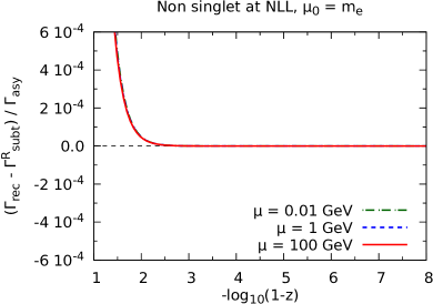
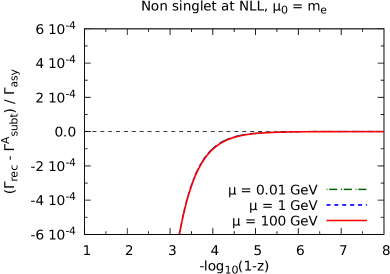
Figure 1: Ratio of the l.h.s. of eq. (135) over its r.h.s. (without the absolute values), for the two choices of the subtraction term (eq. (139), left panel; eq. (140), right panel), and for three different hard-scale values: $\mu=0.01$ GeV (dot-dashed green), $\mu=1$ GeV (dashed blue), and $\mu=100$ GeV (solid red). As is indicated, the scale on the $y$ axis of these plots is in units of $10^{-4}$.

The curves in fig. 1 are relevant to the non-singlet component. We point out that their analogues for the singlet component are qualitatively and quantitatively very similar to those shown here. Apart from being in keeping with the expectations emerging from eqs. (143)–(145), fig. 1 shows that, even in the case of eq. (139), the matched PDF will attain its asymptotic form only for values of $z$ which are extremely close to one; in other words, non-logarithmic contributions are almost always important. This being the case, by choosing $\Gamma_{\rm subt}^{\rm A}(z)$ as a subtraction term rather than $\Gamma_{\rm subt}^{\rm R}(z)$ (which, as was anticipated, “delays” the onset of the asymptotic regime in the matched PDF) one renders the transition between the asymptotic and recursive solutions less abrupt; this turns out to be beneficial in order to reproduce the results of the numerical evolution.

As far as the small- and intermediate-$z$ region is concerned, we observe that:

$$\Gamma_{\rm asy}(z)-\Gamma_{\rm subt}^{\rm R}(z) = {\cal O}(\alpha)\,,$$ (146)

$$\Gamma_{\rm asy}(z)-\Gamma_{\rm subt}^{\rm A}(z) = {\cal O}(\alpha^{4})\,.$$ (147)

Equation (146) implies that it is unlikely that, if the subtraction term is defined by means of the recursive solution, one can avoid the use of the $G(z)$ function. Conversely, eq. (147) implies that the definition by means of the asymptotic solution has a better chance of satisfying eq. (137), thus bypassing the need to introduce $G(z)$. Note that the difference in eq. (147) is of ${\cal O}(\alpha^{4})$ as a direct consequence of the fact that we have computed $\Gamma_{\rm subt}^{\rm A}(z)$ to ${\cal O}(\alpha^{3})$ (see eq. (367)). In fig. 2 we plot the ratio of the l.h.s. over the r.h.s. of eq. (137) (without the absolute values), by using the same layout as in fig. 1.

    

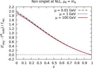
Figure 2: Same as in fig. 1, for eq. (137). As is indicated, the scale on the $y$ axis of the plot on the right panel is in units of $10^{-4}$.

In order to be definite, we have considered again the non-singlet component in fig. 2, and have verified that the singlet one gives results which are extremely similar to those of the non-singlet. Figure 2 confirms our expectation based on eqs. (146) and (147).

We now turn to discussing the case of the photon PDF, which is quite different from that of the singlet and the non-singlet. The starting point is the same as for the latter PDFs, namely the definition of the subtraction term with either eq. (139) or (140), since those formulae are the general parametrisations of the perturbative expansion of the recursive or the asymptotic solutions, respectively, whose actual values are determined by the parameters (given in appendices A.1, A.2, C.1, and C.2) specific to the particle which is being considered. Indeed, in the case of the photon, the analogues of eqs. (141) and (142) are:

$$\Gamma_{\rm subt}^{\rm R}(z)\;\; \longleftrightarrow \;\;\Big{\{}q_{i}(z)\Big{\}}\,,$$ (148)

$$\Gamma_{\rm subt}^{\rm A}(z)\;\; \longleftrightarrow \;\;\Big{\{}q_{i}(z)\Big{\}}\,.$$ (149)

Actually, because of eqs. (386) and (387), one can make a stronger statement, namely:

$$\Gamma_{\rm subt}^{\rm R}(z)=\Gamma_{\rm subt}^{\rm A}(z)\,.$$ (150)

We stress that eq. (150) is not a property inherent to the photon PDF, but a consequence of having been able to keep the relevant subleading terms in the computation of its large-$z$ form as carried out in appendix B. In order to be definite, for consistency with the case of the singlet/non-singlet we shall label the subtraction term with “A” here.

    

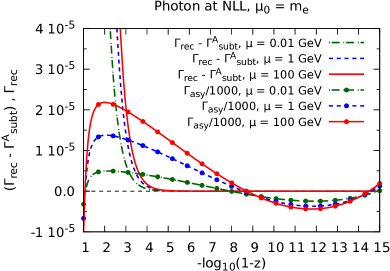
Figure 3: Plots assessing the validity of eq. (137) (left panel) and eq. (135) (right panel), in the case of the photon PDF. See the text for details.

The analogues of the right-hand side panels of fig. 1 and of fig. 2 are presented in the right and left panels of fig. 3, respectively. We start from the right-hand side one, in order to assess the validity of eq. (135). Unfortunately, it turns out that at large $z$’s the NLL photon PDF becomes negative in a certain range, and it crosses twice the zero. For this reason, we cannot consider the ratio of the two sides of eq. (135) as was done in fig. 1, but only plot separately $\Gamma_{\rm rec}(z)-\Gamma_{\rm subt}(z)$ and $\Gamma_{\rm asy}(z)$; these two quantities are displayed in fig. 3 by adopting identical patterns (each associated with a different hard scale $\mu$), with the curves relevant to $\Gamma_{\rm asy}(z)$ overlaid by full circles. Furthermore, in order for the latter curves to fit into the layout, they have been multiplied by a constant factor equal to $10^{-3}$. The plot clearly shows how eq. (135) is safely fulfilled.

We now consider the left panel of fig. 3, in order to assess the validity of eq. (137); given that for all of the $z$ values employed in the plot the photon PDFs is positive, we can compute the ratio of the two sides of eq. (137) (without the absolute values) as was done previously in fig. 2. It is immediate to see that the conclusions are the opposite of those valid in the cases of the singlet and non-singlet – namely, in a very large range in $z$ the subtraction term and the asymptotic solution do not agree with each other. Thus, in the case of the photon the use of a damping function $G(z)$ is unavoidable. In order to define it, it is useful to introduce the function:

$$\hat{z}(z)=-\log_{10}(1-z)\,,$$ (151)

by means of which we set:

$$G(z)=\left\{\begin{array}[]{ll}1&\phantom{aaaa}\hat{z}_{1}\leq\hat{z}(z)\,,\\ G_{p}\!\left(\frac{\hat{z}(z)-\hat{z}_{0}}{\hat{z}_{1}-\hat{z}_{0}}\right)&\phantom{aaaa}\hat{z}_{0}\leq\hat{z}(z)<\hat{z}_{1}\,,\\ 0&\phantom{aaaa}\hat{z}(z)<\hat{z}_{0}\,,\\ \end{array}\right.\;\;\;\;\;\;\;\;\;\;G_{p}(v)=\frac{v^{p}}{v^{p}+(1-v)^{p}}\,.$$ (155)

This is a smooth function that obeys eqs. (132) and (136), and where $\hat{z}_{0}$, $\hat{z}_{1}$, and $p$ are free parameters. The physical meaning of the parameters $\hat{z}_{0}$ and $\hat{z}_{1}$ is that, for $z$ such that $\hat{z}(z)<\hat{z}_{0}$ ($\hat{z}(z)>\hat{z}_{1}$), the matched PDF coincides with the recursive (the asymptotic) solution. As a matter of fact, eqs. (151) and (155) stem from the observation that it is $\hat{z}(z)$, and not $z$, the natural variable to carry out the matching, and this is because the large-$z$ behaviour of the PDFs is achieved when logarithmic terms grow much larger than non-logarithmic ones.

Figure 4: Study of the dependence of the matched photon PDF upon the parameters of the matching function $G(z)$, defined in eq. (155). We have set $\mu=100$ GeV.

In principle, the parameters $\hat{z}_{0}$, $\hat{z}_{1}$, and $p$ are unconstrained. In order to choose them sensibly, we plot in fig. 4 the asymptotic and recursive solutions as solid black and red curves, respectively (both are multiplied by a factor of $10^{-2}$, for reasons that will soon become clear). For the matching to work reasonably well, the transition between the recursive and the asymptotic solutions must occur in a region where these two predictions are as close as possible to each other (which we interpret as the signal that both give a reasonable description of the “true” photon PDF). From fig. 4, we gather that such a region is $2\lesssim\hat{z}\lesssim 6$; this suggests to set $\hat{z}_{0}=2$ and $\hat{z}_{1}=6$. However, it is clear that there is (and there must be) a certain flexibility in these choices. The agreement between the asymptotic and recursive solutions quickly worsens in the range $z\in(1,2)$, which implies that $\hat{z}_{0}=1$ must be considered as an extreme choice. On the other hand, for $\hat{z}>6$ the asymptotic and recursive solutions do tend to stay relatively close to each other, to the extent that even $\hat{z}_{1}=10$ appears to be an acceptable choice. As far as $p$ is concerned, the larger this parameter the more abrupt is the transition between the two regimes. We have therefore opted to employ $p=2$, which essentially corresponds to the slowest transition compatible with the derivatives of $G(z)$ being continuous. In order to assess the impact of the choices of $\hat{z}_{0}$ and $\hat{z}_{1}$ on the matched PDF, we have computed the latter for several values of these parameters. In fig. 4 we display as dashed curves the differences between any of the matched predictions (relevant to $(\hat{z}_{0},\hat{z}_{1})=(1,5)$, $(3,5)$, $(1,7)$, $(3,7)$, and $(1,10)$) minus the one obtained with $(\hat{z}_{0},\hat{z}_{1})=(2,6)$. For comparison, we also show the differences between the asymptotic and recursive solutions minus the $(\hat{z}_{0},\hat{z}_{1})=(2,6)$ matched PDF as black and red dot-dashed curves, respectively. We see that the differences between any two pairs of matched predictions are roughly in the range $(-2,3)\cdot 10^{-4}$, i.e. at least a factor $25$ smaller than the recursive and the asymptotic solutions. While this statement progressively loses validity when moving towards $\hat{z}=8$ (where the asymptotic solution, which is the appropriate one in this region, crosses zero), it also becomes less relevant, since indeed all quantities of interest tend to become negligible in absolute value. Having said that, it is important to bear in mind that the dependence on the matching-function parameters is a genuine uncertainty that affects the matched predictions; plots such as those in fig. 4 help assess its size, and should be re-produced whenever new conditions become relevant (specifically, for hard-scale values significantly different w.r.t. those considered in fig. 4). We finally point out that we have repeated the exercise by using $p=3$ and $p=4$; the overall uncertainties are similar to those obtained with $p=2$.

In summary, our best analytical results are obtained with the matching formula of eq. (131). In the case of the singlet and the non-singlet, we employ eq. (140) for the definition of the subtraction term, and a constant $G(z)$ function as in eq. (138). In the case of the photon, the definition of the subtraction term is still given by eq. (140) – however, there are more limited possibilities here, owing to eq. (150). The matched photon PDF does need a non-trivial matching function: we adopt that of eq. (155), with $\hat{z}_{0}=2$, $\hat{z}_{1}=6$, and $p=2$.

8 Numerical and analytical predictions

In this section we present our predictions for the PDFs, by computing them both with the numerical code described in the first part of sect. 6, and by evaluating the analytical formulae; these are always the matched ones. We compare these two classes of predictions, mutually validating them in the process. Unless explicitly indicated, all results are NLL-accurate with running $\alpha$, and all have been obtained by setting $\mu_{0}=m$.

We begin by plotting in fig. 5 the electron, photon, and positron PDFs, computed at $\mu=100$ GeV with the numerical code. The left panel shows

    

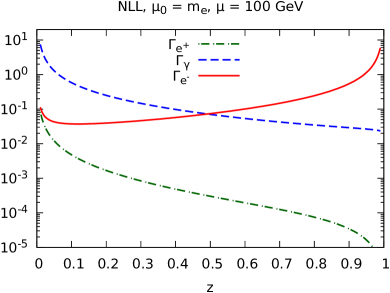
Figure 5: Electron (solid red), photon (dashed blue), and positron PDFs (dot-dashed green) PDFs at $\mu=100$ GeV. The electron PDF is multiplied by a factor $(1-z)$ in the plot on the right panel.

these quantities in the full $z\in(0,1)$ range, while the right panel is a zoom to the large-$z$ region, where we consider $\hat{z}\in(1,15)$ (see eq. (151) for the definition of $\hat{z}$). Owing to the much faster growth of the electron PDFs in this region w.r.t. that of the other two partons, we have multiplied this PDF by a factor equal to $(1-z)$, in order for all of the three curves to fit into the same layout. Figure 5 renders it manifest that the production of heavy (relative to the collider c.m. energy) objects is dominated by the partonic lepton whose charge is the same as that of the particle lepton it stems from (in eq. (1), one has the implicit constraint $z_{+}z_{-}\geq M^{2}/S$, with $M$ and $\sqrt{S}$ the mass of the object produced and the collider c.m. energy, respectively). Note that from the right panel of fig. 5, given that the solid-red and dashed-blue curves are roughly of the same order, and that the former includes the $(1-z)$ factor, one can immediately see that the photon PDF is smaller than the electron PDF by a number of orders of magnitude equal to the value of $\hat{z}$. Conversely, by producing lighter objects and/or by increasing the collider energy, the contribution(s) of the incoming photon(s) become(s) important.

In view of the smallness of the positron PDF as is documented in fig. 5, it is more convenient to present our findings in terms of the singlet and the non-singlet PDFs rather than by means of the electron and positron ones. This is what we shall do in the remainder of this section.

In order to establish the level of agreement between our numerical and analytical predictions, we plot in figures 6, 7, and 8 the ratios of the latter over the former, minus one, in the cases of the non-singlet, singlet, and photon, respectively.

    

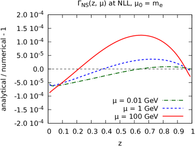
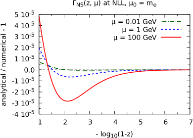
Figure 6: Comparison between the numerical and analytical predictions for the non-singlet, for three different hard-scale choices.

In each plot, there are three curves, corresponding to three different choices of hard scales: $\mu=0.01$ GeV (dot-dashed green curves), $\mu=1$ GeV (dashed blue curves), and $\mu=100$ GeV (solid red curves). An overarching observation is that, in all of the cases bar for the photon at large $z$’s (an exception to which we shall return later), the $\mu=100$ GeV results are those which display the largest analytical-numerical disagreements.

    

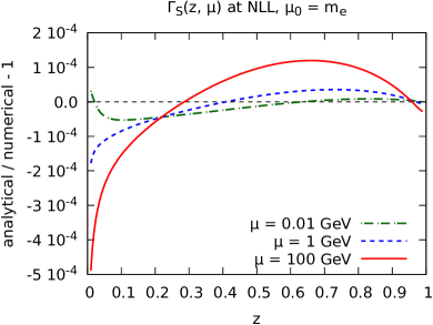
Figure 7: As in fig. 6, for the singlet.

    

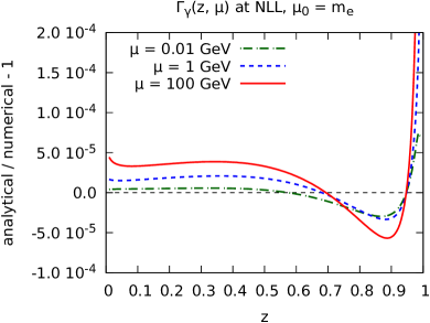
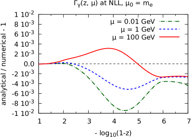
Figure 8: As in fig. 6, for the photon.

However, even in this worst-case scenario, the level of agreement is excellent, being typically of the order of $10^{-5}$–$10^{-4}$ (relative); the largest disagreements are to be found at small $z$’s in the case of the singlet (because of the presence of un-resummed $\log z$ terms). In keeping with the previous remark relevant to the hard-scale dependence, the case of the photon at $z\simeq 1$ constitutes an exception: from the right panel of fig. 8 we see that the analytical and numerical predictions agree at the level of $10^{-3}$ ($10^{-2}$) at $\mu=100$ GeV ($\mu=0.01$ GeV) for $2\lesssim\hat{z}\lesssim 6\,$; furthermore, the behaviour at $\hat{z}>6$ might seem to suggest that the $z\to 1$ limits of the analytical and numerical computations are different. We shall show in the following (see fig. 12) that this is in fact not the case. For the time being, the crucial thing to bear in mind is that, in the $z$ region we are discussing, the photon PDF is very small in absolute value and, more importantly, smaller than the electron PDF by several orders of magnitude. Thus, even a relatively large discrepancy of 0.1–1% between the numerical and analytical photon PDFs will be quite irrelevant. The general conclusion, which applies to all partons, is therefore that the analytical formulae appear to be perfectly adequate, and can be employed in calculations of cross sections for phenomenological purposes.

    

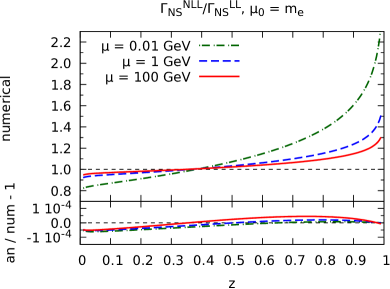
Figure 9: Main frames: ratios of NLL over LL PDF, as computed with the numerical code, for the non-singlet, and for three different hard-scale choices. Insets: ratio of the ratio shown in the main frame, over the same quantity computed analytically, minus one.

    

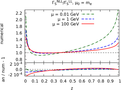
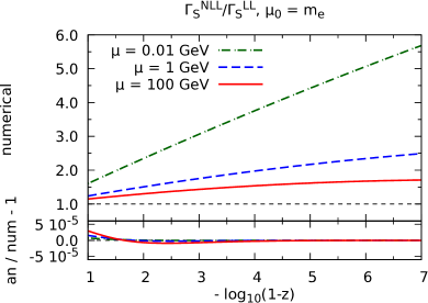
Figure 10: As in fig. 9, for the singlet.

    

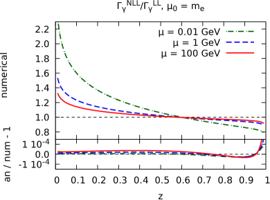
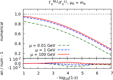
Figure 11: As in fig. 9, for the photon.

We now turn to assessing the effects on the PDFs of the NLL corrections, by comparing the NLL results with their LL counterparts. While this will fully account for the predictions obtained here for the first time, it is important to bear in mind that the PDFs are unphysical quantities, and that beyond LL cancellations do occur (in particular, in $\overline{\rm MS}$) between them and the short-distance cross sections. Thus, an increase or decrease by a factor $X$ of an NLL PDF w.r.t. an LL one will most definitely not translate into a corresponding increase or decrease of the NLO physical cross section w.r.t. its LO counterpart.

In the main frames of figs. 9, 10, and 11, we plot the ratios of the NLL PDFs over the LL ones, both computed with the numerical code. As was done previously, all figures feature three curves, that correspond to different choices of hard scales; the same scale values, and the same graphical patterns, are used here as in figs. 6–8. All the figures have an inset, which displays the double ratio (minus one):

$$\left.\frac{{\rm PDF}_{\scriptscriptstyle\rm NLL}}{{\rm PDF}_{\scriptscriptstyle\rm LL}}\right|_{\rm an}\Bigg{/}\left.\frac{{\rm PDF}_{\scriptscriptstyle\rm NLL}}{{\rm PDF}_{\scriptscriptstyle\rm LL}}\right|_{\rm num}-1\,.$$ (156)

The agreement between the numerical and analytical predictions is again extremely good, especially at large $z$’s; once more, the photon in this region is the (relative) exception to that general rule, on which we shall comment later. The agreement becomes marginally worse with increasing $\mu$, but this effect is less evident w.r.t. that in the case of the absolute predictions of figs. 6–8. Interestingly, the size of the NLL effects decreases with the hard scale. This is particularly easy to understand in the large-$z$ region in the case of the singlet (or non-singlet), since it can be directly read from eq. (113). As was already remarked there, this behaviour is driven by eq. (114), which implies that: a) the coefficient of the $\log(1-z)$ term is much larger than that of the $\log^{2}(1-z)$ term up to extremely large values of $z$; b) such a coefficient, being proportional to $1/\alpha(\mu)$, decreases with $\mu$. These two effects can clearly be seen in the main frames of the right panels of figs. 9 and 10, where the various lines are almost straight ones, but relatively less so at larger values of the hard scales. Keeping in mind the general observation made above on the unphysical nature of the PDFs, we point out that the natural applications of the quantities computed here involve scales that are large.

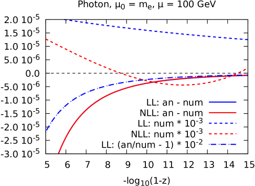
Figure 12: Behaviour of the photon PDF at very large $z$ values, where the analytical and numerical predictions are compared. We have set $\mu=100$ GeV.

We now go back to commenting on the large-$z$ behaviour of the photon PDF. We have already remarked in fig. 8 that such a PDF in this region is close to zero in absolute value, and orders of magnitude smaller than its electron counterpart. On top of that, for the specific issue of the NLL vs LL results, the comparison between eqs. (343) and (357) (or between their over-simplified forms of eqs. (356) and (360)) shows that, at variance with the case of the electron (eqs. (113) and (116)), the NLL asymptotic photon PDF does not factorise the functional form relevant to its LL version. Hence, larger differences in the matching region have to be expected between the NLL and LL photon PDF, which are larger than those for the electron.

At the right end of the $z$ range in fig. 11 we see again the kind of pattern as in the same region of fig. 8, which might cast doubts on the agreement between the $z\to 1$ limits of the analytical and numerical predictions. In order to address this concern, in fig. 12 we plot the photon PDF in a much more extended $z$ range w.r.t. what was done so far. The blue and red solid curves are the differences between the analytical and numerical results computed at the LL and NLL, respectively; the dashed curves of the same colours are the corresponding PDFs, multiplied by an overall constant factor equal to $10^{-3}$; finally, the blue dot-dashed curve is the rescaled ratio of the analytical over the numerical LL results, minus one, which can be sensibly computed owing to the fact that the LL PDF does not vanish for values of $z\neq 1$. Apart from the similarity between the LL and NLL differences, the key message of fig. 12 is that at $z\to 1$ the analytical and numerical predictions do tend to the same value, but in a much slower way w.r.t. the case of the singlet/non-singlet. In other words, the onset of the true asymptotic regime occurs at much larger $z$ values for the photon than for the singlet or non-singlet. This needs not be surprising, owing to the mechanism that governs the asymptotic photon behaviour, as is documented in appendix B. An improvement of the analytical large-$z$ PDF computed here would require keeping all terms suppressed by powers of $N^{-2}$ in Mellin space, an extremely involved computation which is not justified in view of the smallness of the photon PDF in this region.

9 Conclusions

In this paper we have computed the electron, positron, and photon PDFs relevant to an incoming unpolarised electron; the case of an incoming positron is trivially obtained by charge conjugation. Our predictions include up to next-to-leading logarithmic (NLL) terms, and are obtained by evolving the initial conditions that have recently been calculated Frixione:2019lga at the next-to-leading order (NLO). We thus improve upon the long-standing leading-logarithmic (LL) PDFs of refs. Skrzypek:1990qs ; Skrzypek:1992vk ; Cacciari:1992pz ; this is crucial to help achieve the high-precision results needed at future $e^{+}e^{-}$ colliders. All of the calculations are perturbative in the QED coupling constant $\alpha$, which by default we take as running.

The PDFs have been obtained by means of both numerical and analytical methods, which are shown to agree extremely well with each other (typically, at the $10^{-4}$ level or better for those $z$ values where the relevant PDFs are not vanishingly small). As far as the analytical results are concerned, they stem from an additive matching formula (eq. (131)), which combines a prediction that is accurate to all orders in $\alpha$ but only at $z\to 1$, with a prediction that is accurate up to ${\cal O}(\alpha^{3})$ in the whole $z$ range; these are referred to as the asymptotic and the recursive solutions, respectively. The latter are thus called because they stem from recursive equations (derived here for the first time at the NLL accuracy), whereby the ${\cal O}(\alpha^{k})$ contributions are obtained from the ${\cal O}(\alpha^{p})$ ones (with $p<k$), the NLO initial conditions, and the Altarelli-Parisi kernels. Although we have limited ourselves to considering $k\leq 3$ in this work, nothing prevents one from employing the recursive equations to achieve an even higher precision if need be.

The electron LL PDF is extremely peaked towards $z\to 1$, where it features an integrable singularity. The NLL result has the same qualitative behaviour, and in fact the $z\to 1$ singularity is even more pronounced than at the LL because of the presence of additional $\log(1-z)$ terms. While the photon LL PDF vanishes at $z\to 1$, its NLL counterpart grows logarithmically there, thus exhibiting the same enhanced growth at higher orders as the electron. However, one must bear in mind that PDFs are unphysical quantities: in particular, beyond LL they become dependent on the adopted collinear subtraction scheme. In this paper we have worked in $\overline{\rm MS}$, and some of the logarithms mentioned above stem directly from this scheme choice; as such, they will cancel against their counterparts in the short-distance cross sections, so as to have scheme-independent predictions for physical observables.

The analytical knowledge of the PDFs is important to better understand the details of QED collinear dynamics. However, in view of the rapidity of the growth of the electron PDF at $z\to 1$, such a knowledge is also crucial in the context of numerical computations, because it gives one the possibility to adapt in a very tailored manner the integration procedure, which would otherwise be hardly converging.

We finally point out that the PDFs of the photon (understood as an incoming particle), and/or those of any polarised particle, can be dealt with similar techniques as those we have employed here.

Appendix A Results for the recursive solutions

In this appendix we report the results for the $J^{\scriptscriptstyle\rm LL}_{k}$ and $J^{\scriptscriptstyle\rm NLL}_{k}$ basis functions that appear in eq. (85), which we have computed for $0\leq k\leq 3$ and $0\leq k\leq 2$, respectively, i.e. up to ${\cal O}(\alpha^{3})$. We write the actual recursive solution that constitutes one of the main results of this paper, and which we have used in our numerical studies, as follows:

$$\Gamma(z,\mu^{2})=\sum_{k=0}^{k_{\rm max}^{\scriptscriptstyle\rm LL}}\frac{t^{k}}{k!}\,J^{\scriptscriptstyle\rm LL}_{k}(z)+\frac{\alpha(t)}{2\pi}\sum_{k=0}^{k_{\rm max}^{\scriptscriptstyle\rm NLL}}\frac{t^{k}}{k!}\,J^{\scriptscriptstyle\rm NLL}_{k}(z)\,,$$ (157)

with

$$k_{\rm max}^{\scriptscriptstyle\rm LL}=3\,,\;\;\;\;\;\;\;\;k_{\rm max}^{\scriptscriptstyle\rm NLL}=2\,.$$ (158)

We also remind the reader that from eq. (157) one can obtain the solution in the case of non-running $\alpha$, by replacing $J^{\scriptscriptstyle\rm LL}_{k}$ with $I^{\scriptscriptstyle\rm LL}_{k}$ and $J^{\scriptscriptstyle\rm NLL}_{k}$ with $I^{\scriptscriptstyle\rm NLL}_{k}$, where:

$$I^{\scriptscriptstyle\rm LL}_{k}(z) = J^{\scriptscriptstyle\rm LL}_{k}(z)\,,$$ (159)

$$I^{\scriptscriptstyle\rm NLL}_{k}(z) = J^{\scriptscriptstyle\rm NLL}_{k}(z)\big{[}b_{0}\to 0\,,b_{1}\to 0\,,b_{1}/b_{0}\to 0\big{]}\,.$$ (160)

It is convenient, also in view of the matching with the large-$z$ solution, to present the results for the basis functions by writing them as follows:

$$J^{\scriptscriptstyle\rm LL}_{k}(z) = \bar{J}^{\scriptscriptstyle\rm LL}_{k}(z)+\hat{J}^{\scriptscriptstyle\rm LL}_{k}(z)\,,$$ (161)

$$J^{\scriptscriptstyle\rm NLL}_{k}(z) = \bar{J}^{\scriptscriptstyle\rm NLL}_{k}(z)+\hat{J}^{\scriptscriptstyle\rm NLL}_{k}(z)\,.$$ (162)

By definition, $\hat{J}^{\scriptscriptstyle\rm LL}_{k}$ and $\hat{J}^{\scriptscriptstyle\rm NLL}_{k}$ collect all of the terms of $J^{\scriptscriptstyle\rm LL}_{k}$ and $J^{\scriptscriptstyle\rm NLL}_{k}$, respectively, that vanish at $z=1$:

$$\lim_{z\to 1}\hat{J}^{\scriptscriptstyle\rm LL}_{k}(z)=\lim_{z\to 1}\hat{J}^{\scriptscriptstyle\rm NLL}_{k}(z)=0\,.$$ (163)

It then follows that $\bar{J}^{\scriptscriptstyle\rm LL}_{k}$ and $\bar{J}^{\scriptscriptstyle\rm NLL}_{k}$ include all contributions that are either divergent (which then feature all the $\log^{p}(1-z)$ terms) or equal to a non-null constant at $z=1$. Because of this, it is useful to introduce the following auxiliary functions:

$$\ell_{i}(z) = \frac{\log^{i}(1-z)}{1-z}\,,\;\;\;\;\;\;\;\;i\geq 0\,,$$ (164)

$$q_{i}(z) = \log^{i}(1-z)\,,\;\;\;\;\;\;\;\;\;i\geq 0\,,$$ (165)

and write:

$$\bar{J}^{\scriptscriptstyle\rm LL}_{k}(z) = \sum_{i=0}^{i_{\rm max}^{\scriptscriptstyle\rm LL}(k)}\Big{[}\,b_{k,i}^{\scriptscriptstyle\rm LL}\,\ell_{i}(z)+c_{k,i}^{\scriptscriptstyle\rm LL}\,q_{i}(z)\Big{]},\;\;\;\;\;\;\;\;\;\;\;k\geq 1\,,$$ (166)

$$\bar{J}^{\scriptscriptstyle\rm NLL}_{k}(z) = \sum_{i=0}^{i_{\rm max}^{\scriptscriptstyle\rm NLL}(k)}\Big{[}\,b_{k,i}^{\scriptscriptstyle\rm NLL}\,\ell_{i}(z)+c_{k,i}^{\scriptscriptstyle\rm NLL}\,q_{i}(z)\Big{]},\;\;\;\;\;\;\;\;k\geq 0\,.$$ (167)

with:

$$i_{\rm max}^{\scriptscriptstyle\rm LL}(k) = k-1\,,$$ (168)

$$i_{\rm max}^{\scriptscriptstyle\rm NLL}(k) = k+1\,.$$ (169)

In addition to this, one must take into account that, at ${\cal O}(\alpha^{0})$:

$$J^{\scriptscriptstyle\rm LL}_{0}(z)=\bar{J}^{\scriptscriptstyle\rm LL}_{0}(z)=\hat{J}^{\scriptscriptstyle\rm LL}_{0}(z)=0\,.$$ (170)

The contribution to $\Gamma(z)$ that does not vanish at $z\to 1$ is then written as follows:

$$\overline{\Gamma}(z,\mu^{2})=\sum_{k=0}^{k_{\rm max}^{\scriptscriptstyle\rm LL}}\frac{t^{k}}{k!}\,\bar{J}^{\scriptscriptstyle\rm LL}_{k}(z)+\frac{\alpha(t)}{2\pi}\sum_{k=0}^{k_{\rm max}^{\scriptscriptstyle\rm NLL}}\frac{t^{k}}{k!}\,\bar{J}^{\scriptscriptstyle\rm NLL}_{k}(z)\,.$$ (171)

The expressions of the $b_{k,i}^{\scriptscriptstyle\rm(N)LL}$ and $c_{k,i}^{\scriptscriptstyle\rm(N)LL}$ coefficients for the non-singlet, singlet, and photon PDFs will be presented in appendix A.1 (LL results), and in appendix A.2 (NLL results). The expressions of the functions $\hat{J}^{\scriptscriptstyle\rm(N)LL}(z)$ are lengthy (with some of them receiving contributions that we have not computed analytically, as detailed below), and not relevant to the matching; for these reasons, they are only reported in an ancillary file that will accompany the submission of this paper to the arXiv. We remind the reader that the recursive solutions are obtained by following the procedure outlined in sect. 5.1. Namely, one first computes the ${\cal J}^{\scriptscriptstyle\rm LL}_{k}$ and ${\cal J}^{\scriptscriptstyle\rm NLL}_{k}$ functions, by employing eqs. (80) and (5.1). These equations must be applied recursively, by working one’s own way up in $k$ from the known $k=0$ results (given in eqs. (60)–(63)). The expressions for the Altarelli-Parisi kernels are taken from ref. deFlorian:2016gvk . Finally, the $J^{\scriptscriptstyle\rm LL}_{k}$ and $J^{\scriptscriptstyle\rm NLL}_{k}$ functions are obtained by derivation, according to eq. (86).

         

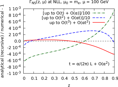
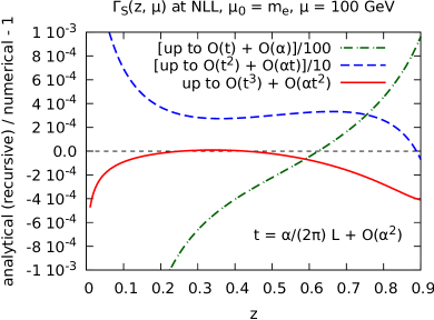
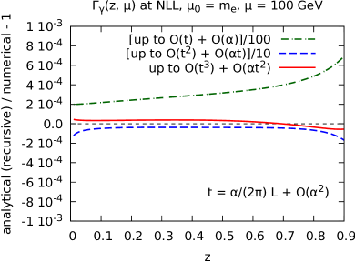
Figure 13: Agreement between recursive solutions of various accuracies, and the numerical predictions, for the non-singlet (top left panel), singlet (top right panel), and photon (bottom panel), for $\mu=100$ GeV. See the text for details.

In order to document the effect of increasing the number of terms included in the recursive solutions, we plot in fig. 13 the ratio of the result of eq. (157) over the numerical predictions minus one; eq. (157) is computed by setting:

$$k_{\rm max}^{\scriptscriptstyle\rm NLL}=k_{\rm max}^{\scriptscriptstyle\rm LL}-1\,,\;\;\;\;\;\;\;\;k_{\rm max}^{\scriptscriptstyle\rm LL}=1,2,3\,.$$ (172)

The ratios are displayed as green dot-dashed lines ($k_{\rm max}^{\scriptscriptstyle\rm LL}=1$), blue dashed lines ($k_{\rm max}^{\scriptscriptstyle\rm LL}=2$), and red solid lines ($k_{\rm max}^{\scriptscriptstyle\rm LL}=3$). In order for the results to fit into the layout of the figures, the green and blue curves are multiplied by a constant factor equal to $10^{-2}$ and $10^{-1}$, respectively. In keeping with what has been discussed in sect. 8, we see that our most accurate recursive predictions ($k_{\rm max}^{\scriptscriptstyle\rm LL}=3$) agree with the numerical results at the level of a few $10^{-4}$ at the worst. Note that since here we are dealing only with the recursive solutions we have limited ourselves to plotting the PDFs in the range $z\in(0,0.9)$ – at the upper end of the range, the absence of the contribution from the asymptotic solution starts to be felt. The new information stemming from fig. 13 is that, if we had only computed either the first term or the first two terms in the sums of eq. (157), the ${\cal O}(10^{-4})$ agreement remarked above would actually have been roughly equal to, but generally worse than, $10^{-2}$ and $10^{-3}$, respectively. The figure also shows that, for any given accuracy of the recursive solution, the agreement with the numerical prediction marginally worsens towards $z\to 0$ in the case of the singlet, owing to the presence of $\log z$ terms which are not resummed.

In the course of the recursive procedure, we have found that some integrals relevant to ${\cal J}^{\scriptscriptstyle\rm NLL}_{2}$ (i.e. the function associated with the ${\cal O}(\alpha t^{2})$ term in the representation of the PDFs) are not easily computable analytically. We have therefore opted to limit ourselves to obtaining their $z\to 1$ leading terms analytically, while evaluating all of the remaining terms numerically, so that the latter contribute only to $\hat{J}^{\scriptscriptstyle\rm NLL}_{2}$ (we point out that an analogous strategy has already been adopted in ref. Cacciari:1992pz ). More precisely, let us consider the generic modified-convolution integral of eq. (53). We distinguish two possibilities: either $g(x)$ is a plus distribution, or it is an ordinary function. Notation-wise, these two cases are written as follows:

$${\rm plus~{}distribution:}\phantom{aaaaaaa}g(x)=\Big{[}\hat{g}(x)\Big{]}_{+}\,,$$ (173)

$${\rm ordinary~{}function:}\phantom{aaaaaa}g(x)\,.$$ (174)

In the case of eq. (173), we have:

$$\big{[}\hat{g}\big{]}_{+}\,\overline{\otimes}\,_{z}h=\left.\big{[}\hat{g}\big{]}_{+}\,\overline{\otimes}\,_{z}h\right|_{\rm end}+\left.\big{[}\hat{g}\big{]}_{+}\,\overline{\otimes}\,_{z}h\right|_{\rm bulk}\,,$$ (175)

where we have defined the endpoint and bulk contributions, respectively, as follows:

$$\left.\big{[}\hat{g}\big{]}_{+}\,\overline{\otimes}\,_{z}h\right|_{\rm end} = -h(z)\int_{0}^{z}dx\,\hat{g}(x)\,,$$ (176)

$$\left.\big{[}\hat{g}\big{]}_{+}\,\overline{\otimes}\,_{z}h\right|_{\rm bulk} = \int_{z}^{1}dx\,\hat{g}(x)\left[h\left(\frac{z}{x}\right)-h(z)\right]$$ (177)

$$= \int_{0}^{1}dy\,(1-z)\,\hat{g}\Big{(}1-(1-z)y\Big{)}\left[h\!\left(\frac{z}{1-(1-z)y}\right)-h(z)\right]\,.\phantom{aa}$$

These equations can also be used in the simpler case of eq. (174): one simply sets the endpoint contribution equal to zero, and computes eq. (177) by removing the subtraction term $h(z)$ and with the formal replacement $\hat{g}\to g$ there.

The endpoint contribution of eq. (176) is always computed analytically, and its results are included in $\bar{J}^{\scriptscriptstyle\rm NLL}_{2}(z)$ and/or $\hat{J}^{\scriptscriptstyle\rm NLL}_{k}(z)$, according to the behaviour of $h(z)$ at $z\to 1$. As far as eq. (177) is concerned, for the sake of the forthcoming discussion let us re-write it more compactly as follows:

$$F(z)=\int_{0}^{1}dy\,f(y,z)\,.$$ (178)

If the integral in eq. (178) were strongly convergent, then we might obtain its contribution to the PDF (see eq. (52)) by means of a derivation under the integral sign, namely:

$$-\frac{\partial F(z)}{\partial z}=-\int_{0}^{1}dy\,\frac{\partial f(y,z)}{\partial z}\,.$$ (179)

Unfortunately, the strong convergence of the integral is not guaranteed, given that $F(z)$ in general is logarithmically divergent at $z\to 1$. However, the contributions that are non vanishing at $z=1$ are also easy to compute analytically; such computation can be carried out directly at the differential level of eq. (179), and stems from expanding the integrand on the r.h.s. of that equation in a series of $z$ around $1$. The latter must include all terms that result in either a logarithmically-divergent or a constant non-null term at $z\to 1$, which typically implies up to $(1-z)^{0}$ contributions. In this way we arrive at the following identity:

$$-\frac{\partial F(z)}{\partial z}=-\left[\frac{\partial F(z)}{\partial z}-\left.\frac{\partial F(z)}{\partial z}\right|_{\rm asy}\right]-\left.\frac{\partial F(z)}{\partial z}\right|_{\rm asy}\,,$$ (180)

with:

$$\left.\frac{\partial F(z)}{\partial z}\right|_{\rm asy}=\int_{0}^{1}dy\,\left.\frac{\partial f(y,z)}{\partial z}\right|_{\rm exp}\,,$$ (181)

having denoted by $\partial f/\partial z|_{\rm exp}$ the aforementioned series expansion. The integral in eq. (181) is computed analytically, and its result added to $\bar{J}^{\scriptscriptstyle\rm NLL}_{2}$ (thus, given eq. (167), it contributes to $c_{2,i}^{\scriptscriptstyle\rm NLL}$ for some $i$, depending on $h(z)$; there are no contributions to $b_{2,i}^{\scriptscriptstyle\rm NLL}$):

$$-\left.\frac{\partial F(z)}{\partial z}\right|_{\rm asy}\;\longrightarrow\;\bar{J}^{\scriptscriptstyle\rm NLL}_{2}(z)\,.$$ (182)

Conversely, the quantity in square brackets in eq. (180), where the rightmost term is regarded as a regularising factor, is computed numerically, and eventually included in $\hat{J}^{\scriptscriptstyle\rm NLL}_{2}$:

$$-\left[\frac{\partial F(z)}{\partial z}-\left.\frac{\partial F(z)}{\partial z}\right|_{\rm asy}\right]\equiv-\int_{0}^{1}dy\,\left(\frac{\partial f(y,z)}{\partial z}-\left.\frac{\partial f(y,z)}{\partial z}\right|_{\rm exp}\right)\;\longrightarrow\;\hat{J}^{\scriptscriptstyle\rm NLL}_{2}(z)\,.$$ (183)

We list here the pairs $\hat{g}$ (or $g$) and $h$ that we handle in the way we have just described:

$$\hat{g}_{a}(v) =\frac{1+v^{2}}{1-v}\,, \quad h_{a}(v) =\log^{2}(1-v)\log v\,,$$ (184)

$$\hat{g}_{b}(v) =\frac{1+v^{2}}{1-v}\,, \quad h_{b}(v) =\log(1-v)\,\text{Li}_{2}(v)\,,$$ (185)

$$\hat{g}_{c}(v) =\frac{1+v^{2}}{1-v}\,, \quad h_{c}(v) =\log^{2}(v)\,\log(1+v)\,,$$ (186)

$$\hat{g}_{d}(v) =\frac{1+v^{2}}{1-v}\,, \quad h_{d}(v) =\log(v)\,\log^{2}(1+v)\,,$$ (187)

$$\hat{g}_{e}(v) =\frac{1+v^{2}}{1-v}\,, \quad h_{e}(v) =\log(v)\,\text{Li}_{2}(-v)\,,$$ (188)

$$\hat{g}_{f}(v) =\frac{1+v^{2}}{1-v}\,, \quad h_{f}(v) =\log(1+v)\,\text{Li}_{2}(-v)\,,$$ (189)

$$\hat{g}_{g}(v) =\frac{1+v^{2}}{1-v}\,, \quad h_{g}(v) =\log(1+v)\,\text{Li}_{2}\left(\frac{1}{1+v}\right)\,,$$ (190)

$$\hat{g}_{h}(v) =\frac{1+v^{2}}{1-v}\,, \quad h_{h}(v) =\text{Li}_{3}(1-v)\,,$$ (191)

$$\hat{g}_{i}(v) =\frac{1+v^{2}}{1-v}\,, \quad h_{i}(v) =\text{Li}_{3}(-v)\,,$$ (192)

$$\hat{g}_{j}(v) =\frac{1+v^{2}}{1-v}\,, \quad h_{j}(v) =\text{Li}_{3}\left(\frac{1}{1+v}\right)\,,$$ (193)

$$\hat{g}_{k}(v) =\frac{1+v^{2}}{1-v}\,\log(1-v)\,\log v\,, \quad h_{k}(v) =\log(1-v)\,,$$ (194)

$$g_{l}(v) =\frac{1+v^{2}}{1+v}\,\log^{2}v\,, \quad h_{l}(v) =\log(1-v)\,,$$ (195)

$$g_{m}(v) =\frac{1+v^{2}}{1+v}\,\log v\,\log(1+v)\,, \quad h_{m}(v) =\log(1-v)\,,$$ (196)

$$g_{n}(v) =\frac{1+v^{2}}{1+v}\,\text{Li}_{2}(-v)\,, \quad h_{n}(v) =\log(1-v)\,,$$ (197)

$$g_{o}(v) =\frac{1}{v}\,, \quad h_{o}(v) =\log v\,\log^{2}(1+v)\,,$$ (198)

$$g_{p}(v) =\frac{1}{v}\,, \quad h_{p}(v) =\log(1+v)\,\text{Li}_{2}(-v)\,,$$ (199)

$$g_{q}(v) =\frac{1}{v}\,, \quad h_{q}(v) =\log(1+v)\,\text{Li}_{2}\left(\frac{1}{1+v}\right)\,,$$ (200)

$$g_{r}(v) =1\,, \quad h_{r}(v) =\text{Li}_{3}(1-v)\,,$$ (201)

$$g_{s}(v) =\frac{1}{v}\,, \quad h_{s}(v) =\text{Li}_{3}(1-v)\,,$$ (202)

$$g_{t}(v) =1\,, \quad h_{t}(v) =\text{Li}_{3}\left(\frac{1}{1+v}\right)\,,$$ (203)

$$g_{u}(v) =\frac{1}{v}\,, \quad h_{u}(v) =\text{Li}_{3}\left(\frac{1}{1+v}\right)\,,$$ (204)

$$g_{v}(v) =\frac{1}{v}\log^{2}(1-v)\,, \quad h_{v}(v) =\log(1-v)\,.$$ (205)

We stress again that each of these pairs will contribute to both eq. (182) and (183). We denote generically either of these contributions as follows:

$$J^{\scriptscriptstyle\rm num}_{\rho}(z)\;\longleftrightarrow\;\big{(}\hat{g}_{\rho},h_{\rho}\big{)}\;\;\;\;{\rm or}\;\;\;\;\big{(}g_{\rho},h_{\rho}\big{)}\,,\;\;\;\;\;\;\;\;\rho=a,\ldots v\,.$$ (206)

These will enter $\bar{J}^{\scriptscriptstyle\rm NLL}_{2}(z)$ and $\hat{J}^{\scriptscriptstyle\rm NLL}_{2}(z)$ as linear combinations with identical coefficients (owing to eq. (180)), which however do depend on the flavour structure. Explicitly:

$${\rm non-singlet:}~{}~{}~{}~{} \sum_{\rho}w_{{\rm\scriptscriptstyle NS},\rho}\,J^{\scriptscriptstyle\rm num}_{\rho}(z)=$$

$$\phantom{aaaa}4\,J^{\scriptscriptstyle\rm num}_{a}+4\,J^{\scriptscriptstyle\rm num}_{b}+4\,J^{\scriptscriptstyle\rm num}_{h}+2\,J^{\scriptscriptstyle\rm num}_{c}+4\,J^{\scriptscriptstyle\rm num}_{d}+4\,J^{\scriptscriptstyle\rm num}_{e}+4\,J^{\scriptscriptstyle\rm num}_{f}$$

$$\phantom{aa}\!-4\,J^{\scriptscriptstyle\rm num}_{g}-4\,J^{\scriptscriptstyle\rm num}_{i}+8\,J^{\scriptscriptstyle\rm num}_{j}-4\,J^{\scriptscriptstyle\rm num}_{k}-2\,J^{\scriptscriptstyle\rm num}_{l}+8\,J^{\scriptscriptstyle\rm num}_{m}+8\,J^{\scriptscriptstyle\rm num}_{n}\,,$$

$${\rm singlet:}~{}~{}~{}~{} \sum_{\rho}w_{{\rm\scriptscriptstyle S},\rho}\,J^{\scriptscriptstyle\rm num}_{\rho}(z)=$$

$$\phantom{aaaa}4\,J^{\scriptscriptstyle\rm num}_{a}+4\,J^{\scriptscriptstyle\rm num}_{b}+4\,J^{\scriptscriptstyle\rm num}_{h}-2\,J^{\scriptscriptstyle\rm num}_{c}-4\,J^{\scriptscriptstyle\rm num}_{d}-4\,J^{\scriptscriptstyle\rm num}_{e}-4\,J^{\scriptscriptstyle\rm num}_{f}$$

$$\phantom{aa}\!+4\,J^{\scriptscriptstyle\rm num}_{g}+4\,J^{\scriptscriptstyle\rm num}_{i}-8\,J^{\scriptscriptstyle\rm num}_{j}-4\,J^{\scriptscriptstyle\rm num}_{k}+2\,J^{\scriptscriptstyle\rm num}_{l}-8\,J^{\scriptscriptstyle\rm num}_{m}$$

$$\phantom{aa}\!-8\,J^{\scriptscriptstyle\rm num}_{n}-24\,n_{\scriptscriptstyle F}\,J^{\scriptscriptstyle\rm num}_{r}\,,$$

$${\rm photon:}~{}~{}~{}~{} \sum_{\rho}w_{\gamma,\rho}\,J^{\scriptscriptstyle\rm num}_{\rho}(z)=$$

$$\phantom{aa}-8\,J^{\scriptscriptstyle\rm num}_{o}-8\,J^{\scriptscriptstyle\rm num}_{p}+8\,J^{\scriptscriptstyle\rm num}_{q}+8\,J^{\scriptscriptstyle\rm num}_{s}+16\,J^{\scriptscriptstyle\rm num}_{t}-16\,J^{\scriptscriptstyle\rm num}_{u}-4\,J^{\scriptscriptstyle\rm num}_{v}\,.$$

The results of these linear combinations when the $J^{\scriptscriptstyle\rm num}_{\rho}$ contributions are computed analytically as in eq. (182) are the following:

$$\sum_{\rho}w_{{\rm\scriptscriptstyle NS},\rho}\,J^{\scriptscriptstyle\rm num}_{\rho}(z) = -\frac{2}{3}\pi^{2}\log(1-z)+\frac{4}{3}\pi^{2}+10\log(2)^{2}\,,$$ (210)

$$\sum_{\rho}w_{{\rm\scriptscriptstyle S},\rho}\,J^{\scriptscriptstyle\rm num}_{\rho}(z) = \frac{2}{3}\pi^{2}\log(1-z)+4\pi^{2}-10\log(2)^{2}\,,$$ (211)

$$\sum_{\rho}w_{\gamma,\rho}\,J^{\scriptscriptstyle\rm num}_{\rho}(z) = -4\log^{3}(1-z)+\frac{4}{3}\pi^{2}\log(1-z)+\frac{4}{3}\pi^{2}\log(2)-4\log(2)^{3}-8\zeta_{3}\,.$$

As was anticipated, the results on the r.h.s. of eqs. (210)–(LABEL:resjbNLL2numga) do not contribute to any of the $b_{2,i}^{\scriptscriptstyle\rm NLL}$ coefficients, while they enter the coefficients $c_{2,1}^{\scriptscriptstyle\rm NLL}$ and $c_{2,0}^{\scriptscriptstyle\rm NLL}$ (singlet and non-singlet), and $c_{2,3}^{\scriptscriptstyle\rm NLL}$, $c_{2,1}^{\scriptscriptstyle\rm NLL}$, and $c_{2,0}^{\scriptscriptstyle\rm NLL}$ (photon).

A.1 LL coefficients

In this appendix we report the results for the coefficients that enter eq. (166); all of the coefficients that do not appear below are understood to be equal to zero.

$\bullet$ Non-singlet:

$$b_{{\rm\scriptscriptstyle NS},\,1,0}^{\scriptscriptstyle\rm LL}=2\,,$$ (213)

$$c_{{\rm\scriptscriptstyle NS},\,1,0}^{\scriptscriptstyle\rm LL}=-2\,,$$ (214)

$$b_{{\rm\scriptscriptstyle NS},\,2,1}^{\scriptscriptstyle\rm LL}=8\,,$$ (215)

$$c_{{\rm\scriptscriptstyle NS},\,2,1}^{\scriptscriptstyle\rm LL}=-8\,,$$ (216)

$$b_{{\rm\scriptscriptstyle NS},\,2,0}^{\scriptscriptstyle\rm LL}=6\,,$$ (217)

$$c_{{\rm\scriptscriptstyle NS},\,2,0}^{\scriptscriptstyle\rm LL}=-2\,,$$ (218)

$$b_{{\rm\scriptscriptstyle NS},\,3,2}^{\scriptscriptstyle\rm LL}=24\,,$$ (219)

$$c_{{\rm\scriptscriptstyle NS},\,3,2}^{\scriptscriptstyle\rm LL}=-24\,,$$ (220)

$$b_{{\rm\scriptscriptstyle NS},\,3,1}^{\scriptscriptstyle\rm LL}=36\,,$$ (221)

$$c_{{\rm\scriptscriptstyle NS},\,3,1}^{\scriptscriptstyle\rm LL}=-12\,,$$ (222)

$$b_{{\rm\scriptscriptstyle NS},\,3,0}^{\scriptscriptstyle\rm LL}=\frac{27}{2}-4\pi^{2}\,,$$ (223)

$$c_{{\rm\scriptscriptstyle NS},\,3,0}^{\scriptscriptstyle\rm LL}=\frac{9}{2}+4\pi^{2}\,.$$ (224)

$\bullet$ Singlet:

$$b_{{\rm\scriptscriptstyle S},\,k,i}^{\scriptscriptstyle\rm LL} = b_{{\rm\scriptscriptstyle NS},\,k,i}^{\scriptscriptstyle\rm LL}\;\;\;\;\;\;\;\;\forall\,k\,,i\,,$$ (225)

$$c_{{\rm\scriptscriptstyle S},\,k,i}^{\scriptscriptstyle\rm LL} = c_{{\rm\scriptscriptstyle NS},\,k,i}^{\scriptscriptstyle\rm LL}\;\;\;\;\;\;\;\;\forall\,k\,,i\,.$$ (226)

$\bullet$ Photon:

$$c_{\gamma,\,1,0}^{\scriptscriptstyle\rm LL}=1\,,$$ (227)

$$c_{\gamma,\,2,1}^{\scriptscriptstyle\rm LL}=2\,,$$ (228)

$$c_{\gamma,\,2,0}^{\scriptscriptstyle\rm LL}=\frac{3}{2}-\frac{2}{3}n_{\scriptscriptstyle F}\,,$$ (229)

$$c_{\gamma,\,3,2}^{\scriptscriptstyle\rm LL}=4\,,$$ (230)

$$c_{\gamma,\,3,1}^{\scriptscriptstyle\rm LL}=6-\frac{4}{3}n_{\scriptscriptstyle F}\,,$$ (231)

$$c_{\gamma,\,3,0}^{\scriptscriptstyle\rm LL}=\frac{9}{4}-\frac{2}{3}\pi^{2}-n_{\scriptscriptstyle F}+\frac{4}{9}n_{\scriptscriptstyle F}^{2}\,.$$ (232)

A.2 NLL coefficients

In this appendix we report the results for the coefficients that enter eq. (167). Note that these do already include the r.h.s. of eqs. (210)–(LABEL:resjbNLL2numga); all of the coefficients that do not appear below are understood to be equal to zero. We employ the following shorthand notation:

$$L_{0}=\log\frac{\mu_{0}^{2}}{m^{2}}\,.$$ (233)

$\bullet$ Non-singlet:

$$b_{{\rm\scriptscriptstyle NS},\,0,1}^{\scriptscriptstyle\rm NLL}=-4\,,$$ (234)

$$c_{{\rm\scriptscriptstyle NS},\,0,1}^{\scriptscriptstyle\rm NLL}=4\,,$$ (235)

$$b_{{\rm\scriptscriptstyle NS},\,0,0}^{\scriptscriptstyle\rm NLL}=2\,(L_{0}-1)\,,$$ (236)

$$c_{{\rm\scriptscriptstyle NS},\,0,0}^{\scriptscriptstyle\rm NLL}=-2\,(L_{0}-1)\,,$$ (237)

$$b_{{\rm\scriptscriptstyle NS},\,1,2}^{\scriptscriptstyle\rm NLL}=-12\,,$$ (238)

$$c_{{\rm\scriptscriptstyle NS},\,1,2}^{\scriptscriptstyle\rm NLL}=12\,,$$ (239)

$$b_{{\rm\scriptscriptstyle NS},\,1,1}^{\scriptscriptstyle\rm NLL}=-14+8L_{0}+8\pi b_{0}\,,$$ (240)

$$c_{{\rm\scriptscriptstyle NS},\,1,1}^{\scriptscriptstyle\rm NLL}=10-8L_{0}-8\pi b_{0}\,,$$ (241)

$$b_{{\rm\scriptscriptstyle NS},\,1,0}^{\scriptscriptstyle\rm NLL}=1-\frac{20}{9}n_{\scriptscriptstyle F}+4\pi b_{0}-\frac{4\pi b_{1}}{b_{0}}+\frac{4}{3}\pi^{2}+L_{0}(6-4\pi b_{0})\,,$$ (242)

$$c_{{\rm\scriptscriptstyle NS},\,1,0}^{\scriptscriptstyle\rm NLL}=-2+\frac{32}{9}n_{\scriptscriptstyle F}-4\pi b_{0}+\frac{4\pi b_{1}}{b_{0}}-\frac{4}{3}\pi^{2}+L_{0}(-2+4\pi b_{0})\,,$$ (243)

$$b_{{\rm\scriptscriptstyle NS},\,2,3}^{\scriptscriptstyle\rm NLL}=-32\,,$$ (244)

$$c_{{\rm\scriptscriptstyle NS},\,2,3}^{\scriptscriptstyle\rm NLL}=32\,,$$ (245)

$$b_{{\rm\scriptscriptstyle NS},\,2,2}^{\scriptscriptstyle\rm NLL}=12(-5+2L_{0}+4\pi b_{0})\,,$$ (246)

$$c_{{\rm\scriptscriptstyle NS},\,2,2}^{\scriptscriptstyle\rm NLL}=-12(-3+2L_{0}+4\pi b_{0})\,,$$ (247)

$$b_{{\rm\scriptscriptstyle NS},\,2,1}^{\scriptscriptstyle\rm NLL}=-17-\frac{160}{9}n_{\scriptscriptstyle F}+56\pi b_{0}-\frac{32\pi b_{1}}{b_{0}}+\frac{40}{3}\pi^{2}-16\pi^{2}b_{0}^{2}-4L_{0}(-9+8\pi b_{0})\,,$$ (248)

$$c_{{\rm\scriptscriptstyle NS},\,2,1}^{\scriptscriptstyle\rm NLL}=-7+\frac{208}{9}n_{\scriptscriptstyle F}-32\pi b_{0}+\frac{32\pi b_{1}}{b_{0}}-\frac{40}{3}\pi^{2}+16\pi^{2}b_{0}^{2}+4L_{0}(-3+8\pi b_{0})\,,$$ (249)

$$b_{{\rm\scriptscriptstyle NS},\,2,0}^{\scriptscriptstyle\rm NLL} = 9-\frac{24\pi b_{1}}{b_{0}}-4\pi b_{0}+6\pi^{2}+8\pi^{2}b_{1}-8\pi^{2}b_{0}^{2}-\frac{16}{3}\pi^{3}b_{0}-40\zeta_{3}$$ (250)

$$+L_{0}\left(\frac{27}{2}-24\pi b_{0}-4\pi^{2}+8\pi^{2}b_{0}^{2}\right)+n_{\scriptscriptstyle F}\left(\frac{40\pi b_{0}}{9}-\frac{2}{9}(33+4\pi^{2})\right),\phantom{aa}$$

$$c_{{\rm\scriptscriptstyle NS},\,2,0}^{\scriptscriptstyle\rm NLL} = -4-\frac{10}{3}\pi^{2}+8\pi^{2}b_{0}^{2}+\frac{8\pi b_{1}}{b_{0}}-8\pi^{2}b_{1}+14\pi b_{0}+\frac{16}{3}\pi^{3}b_{0}$$ (251)

$$+n_{\scriptscriptstyle F}\left(\frac{22}{9}-\frac{64}{9}\pi b_{0}+\frac{8}{9}\pi^{2}\right)+L_{0}\left(\frac{9}{2}+8\pi b_{0}+4\pi^{2}-8\pi^{2}b_{0}^{2}\right)+40\zeta_{3}\,.\phantom{aa}$$

$\bullet$ Singlet:

$$b_{{\rm\scriptscriptstyle S},\,k,i}^{\scriptscriptstyle\rm NLL} = b_{{\rm\scriptscriptstyle NS},\,k,i}^{\scriptscriptstyle\rm NLL}\;\;\;\;\;\;\;\;\forall\,k\,,i\,,$$ (252)

$$c_{{\rm\scriptscriptstyle S},\,k,i}^{\scriptscriptstyle\rm NLL} = c_{{\rm\scriptscriptstyle NS},\,k,i}^{\scriptscriptstyle\rm NLL}\;\;\;\;\;\;\;\;\forall\,k\,,i\,.$$ (253)

$\bullet$ Photon:

$$c_{\gamma,\,0,0}^{\scriptscriptstyle\rm NLL}=(L_{0}-1)\,,$$ (254)

$$c_{\gamma,\,1,2}^{\scriptscriptstyle\rm NLL}=-3\,,$$ (255)

$$c_{\gamma,\,1,1}^{\scriptscriptstyle\rm NLL}=-7+2L_{0}-\frac{4}{3}n_{\scriptscriptstyle F}\,,$$ (256)

$$c_{\gamma,\,1,0}^{\scriptscriptstyle\rm NLL}=-4+n_{\scriptscriptstyle F}\left(-\frac{26}{9}-\frac{2}{3}L_{0}\right)+2\pi b_{0}-\frac{2\pi b_{1}}{b_{0}}+L_{0}\left(\frac{3}{2}-2\pi b_{0}\right)\,,$$ (257)

$$c_{\gamma,\,2,3}^{\scriptscriptstyle\rm NLL}=-6\,,$$ (258)

$$c_{\gamma,\,2,2}^{\scriptscriptstyle\rm NLL}=-\frac{37}{2}+4L_{0}-\frac{2}{3}n_{\scriptscriptstyle F}+10\pi b_{0}\,,$$ (259)

$$c_{\gamma,\,2,1}^{\scriptscriptstyle\rm NLL} = -\frac{37}{2}+\frac{8}{9}n_{\scriptscriptstyle F}^{2}+18\pi b_{0}-\frac{8\pi b_{1}}{b_{0}}+2\pi^{2}$$ (260)

$$+L_{0}(6-8\pi b_{0})-\frac{4}{3}n_{\scriptscriptstyle F}\left(5+L_{0}-2\pi b_{0}\right)\,,$$

$$c_{\gamma,\,2,0}^{\scriptscriptstyle\rm NLL} = -\frac{45}{8}+\left(\frac{52}{27}+\frac{4}{9}L_{0}\right)n_{\scriptscriptstyle F}^{2}+4\pi b_{0}+\frac{11}{6}\pi^{2}-4\pi^{2}b_{0}^{2}-\frac{6\pi b_{1}}{b_{0}}+4\pi^{2}b_{1}$$ (261)

$$+n_{\scriptscriptstyle F}\left(-\frac{23}{6}+\frac{40\pi b_{0}}{9}+\frac{8\pi b_{1}}{3b_{0}}+\frac{2}{9}\pi^{2}-L_{0}+L_{0}\frac{8\pi b_{0}}{3}\right)$$

$$+L_{0}\left(\frac{9}{4}-6\pi b_{0}-\frac{2}{3}\pi^{2}+4\pi^{2}b_{0}^{2}\right)-6\zeta_{3}\,.$$

Appendix B Asymptotic large-$z$ solution for photon PDF beyond leading $N$

In this appendix we consider the problem that has been anticipated in sect. 5.2.3, namely the improvement of the asymptotic behaviour of the photon PDF given in eq. (123) stemming from the inclusion of the off-diagonal elements in the evolution kernels. In order to do this, we start from writing the ${\cal O}(\alpha)$ expressions of the Altarelli-Parisi kernels as follows (see eq. (34)):

$${\mathbb{P}}_{{\rm\scriptscriptstyle S},N} = {\mathbb{P}}_{{\rm\scriptscriptstyle S},N}^{[0]}+\frac{\alpha(\mu)}{2\pi}{\mathbb{P}}_{{\rm\scriptscriptstyle S},N}^{[1]}+{\cal O}(\alpha^{2})$$ (263)

$$\equiv \left({\mathbb{P}}_{{\rm\scriptscriptstyle S},N}^{[0,0]}+\frac{1}{N}{\mathbb{P}}_{{\rm\scriptscriptstyle S},N}^{[0,1]}+{\cal O}\left(N^{-2}\right)\right)$$

$$\phantom{aaa}+\frac{\alpha(\mu)}{2\pi}\left({\mathbb{P}}_{{\rm\scriptscriptstyle S},N}^{[1,0]}+\frac{1}{N}{\mathbb{P}}_{{\rm\scriptscriptstyle S},N}^{[1,1]}+{\cal O}\left(N^{-2}\right)\right)+{\cal O}(\alpha^{2})\,,$$

having introduced, at each order in $\alpha$, the leading- and subleading-$N$ contributions. They read as follows:

$${\mathbb{P}}_{{\rm\scriptscriptstyle S},N}^{[0,0]} = \left(\begin{array}[]{cc}-2\log\bar{N}+2\lambda_{0}&0\\ 0&-\frac{2}{3}\,n_{\scriptscriptstyle F}\\ \end{array}\right),$$ (266)

$${\mathbb{P}}_{{\rm\scriptscriptstyle S},N}^{[0,1]} = \left(\begin{array}[]{cc}-1{}{}&2n_{\scriptscriptstyle F}\\ 1&0\\ \end{array}\right),$$ (269)

$${\mathbb{P}}_{{\rm\scriptscriptstyle S},N}^{[1,0]} = \left(\begin{array}[]{cc}\frac{20}{9}n_{\scriptscriptstyle F}\log\bar{N}+\lambda_{1}&0\\ 0&-n_{\scriptscriptstyle F}\\ \end{array}\right),$$ (272)

$${\mathbb{P}}_{{\rm\scriptscriptstyle S},N}^{[1,1]} = \left(\begin{array}[]{cc}-4\log\bar{N}+\frac{27+22n_{\scriptscriptstyle F}}{9}{}{}{}{}&2n_{\scriptscriptstyle F}\left(\log^{2}\bar{N}+\frac{15-\pi^{2}}{6}\right)\\ -\log^{2}\bar{N}+\frac{15+4n_{\scriptscriptstyle F}}{3}\log\bar{N}-\frac{64n_{\scriptscriptstyle F}+3(36+\pi^{2})}{18}&0\\ \end{array}\right).$$ (275)

Note that, by considering only eqs. (266) and (272), one recovers eq. (121). According to eq. (44), the Altarelli-Parisi kernels define the evolution kernel as follows:

$${\mathbb{M}}_{N}={\mathbb{P}}_{{\rm\scriptscriptstyle S},N}^{[0]}+\frac{\alpha(\mu)}{2\pi}\left({\mathbb{P}}_{{\rm\scriptscriptstyle S},N}^{[1]}-\frac{2\pi b_{1}}{b_{0}}\,{\mathbb{P}}_{{\rm\scriptscriptstyle S},N}^{[0]}\right)\,,$$ (276)

whence one can write the evolution equation and its formal solution as follows:

$$\frac{\partial{\mathbb{E}}_{N}(t)}{\partial t}={\mathbb{M}}_{N}(t){\mathbb{E}}_{N}(t)\;\;\;\;\;\;\Longrightarrow\;\;\;\;\;\;{\mathbb{E}}_{N}(t)=\exp\left[\sum_{k=1}^{\infty}\Omega_{k,N}(t)\right]\,.$$ (277)

The solution in eq. (277) is based on the so-called Magnus expansion Magnus:1954 (see also ref. Magnus:rev2008 ), which is constructed solely in terms of the evolution kernel:

$$\Omega_{1,N}(t) = \int_{0}^{t}dt_{1}{\mathbb{M}}_{N}(t_{1})\,,$$ (278)

$$\Omega_{2,N}(t) = \frac{1}{2}\int_{0}^{t}dt_{1}\int_{0}^{t_{1}}dt_{2}\Big{[}{\mathbb{M}}_{N}(t_{1}),{\mathbb{M}}_{N}(t_{2})\Big{]}\,,$$ (279)

$$\Omega_{3,N}(t) = \ldots\,,$$ (280)

with $\Omega_{k,N}(t)$ featuring $k$ instances of ${\mathbb{M}}_{N}$, all appearing in commutators. Thus, in the case of a one-dimensional flavour space or of a diagonal evolution kernels, eq. (277) is identical to the solutions given in eq. (46) and in sect. 5.2.3. As far as the singlet-photon sector is concerned, we can indeed recover the solutions we have found previously in terms of the quantity introduced in this appendix. We define the leading-$N$ evolution kernel:

$${\mathbb{M}}_{N}^{(0)}={\mathbb{P}}_{{\rm\scriptscriptstyle S},N}^{[0,0]}+\frac{\alpha(\mu)}{2\pi}\left({\mathbb{P}}_{{\rm\scriptscriptstyle S},N}^{[1,0]}-\frac{2\pi b_{1}}{b_{0}}\,{\mathbb{P}}_{{\rm\scriptscriptstyle S},N}^{[0,0]}\right)$$ (281)

and denote by ${\mathbb{E}}_{N}^{(0)}(t)$ the corresponding evolution operator. Thus:

$$\frac{\partial{\mathbb{E}}_{N}^{(0)}(t)}{\partial t}={\mathbb{M}}_{N}^{(0)}(t){\mathbb{E}}_{N}^{(0)}(t)\;\;\;\;\;\;\Longrightarrow\;\;\;\;\;\;{\mathbb{E}}_{N}^{(0)}(t)=\left(\begin{array}[]{cc}E_{\Sigma\Sigma,N}^{(0)}&0\\ 0&E_{\gamma\gamma,N}^{(0)}\\ \end{array}\right),$$ (282)

where:

$$E_{\Sigma\Sigma,N}^{(0)} = \exp\left[-\xi_{1}\log\bar{N}+\hat{\xi}_{1}\right],$$ (283)

$$E_{\gamma\gamma,N}^{(0)} = \exp\left[-\frac{2n_{\scriptscriptstyle F}}{3}t-\frac{\alpha(\mu)-\alpha(\mu_{0})}{4\pi^{2}b_{0}}n_{\scriptscriptstyle F}\Big{(}1-\frac{4\pi b_{1}}{3b_{0}}\Big{)}\right]$$ (284)

$$= \left(\frac{\alpha(\mu_{0})}{\alpha(\mu)}\right)^{\frac{n_{\scriptscriptstyle F}}{3\pi b_{0}}}\exp\left[-\frac{\alpha(\mu)-\alpha(\mu_{0})}{4\pi^{2}b_{0}}n_{\scriptscriptstyle F}\Big{(}1-\frac{4\pi b_{1}}{3b_{0}}\Big{)}\right]\;\stackrel{{\scriptstyle{\rm QED}}}{{\longrightarrow}}\;\frac{\alpha(\mu_{0})}{\alpha(\mu)}\,.$$ (285)

Equation (283) coincides with eq. (100), while eq. (284) coincides with eq. (122), as they should. This is not immediately apparent in the case of eq. (284) since there, at variance with what has been done in eq. (122), we have not used the simplifications induced by the explicit expressions of the QED $\beta$-function coefficients (see eq. (41)). This is useful when one considers the limit of non-running $\alpha$ of the formulae presented here. An expression equivalent to eq. (284), as well as the QED “limit” of both, is given in eq. (285).

We stress that the case of non-running $\alpha$ is problematic, as it might lead to inconsistencies. By switching off the running, one effectively neglects bubble-diagram contributions which are exactly the same as those that lead to the $\gamma\gamma$ entries in eqs. (266) and (272). In this paper we ignore such potential inconsistencies, but then we need to carefully distinguish the $\gamma\gamma$ contributions to the Altarelli-Parisi kernels (which we always parametrise by means of $n_{\scriptscriptstyle F}$) from those to the QED $\beta$ function (which we parametrise by means of the $\beta$-function coefficients $b_{i}$). We shall return to this point with one explicit example later in this appendix (see eqs. (344) and (345)).

In order to improve on the leading-$N$ results, we shall introduce the subleading-$N$ contributions to the evolution kernel, and treat them as a perturbation to the solution of eq. (282). This entails writing:

$${\mathbb{M}}_{N}={\mathbb{M}}_{N}^{(0)}+\frac{1}{N}{\mathbb{M}}_{N}^{(1)}\;\;\;\;\;\;\Longrightarrow\;\;\;\;\;\;{\mathbb{E}}_{N}(t)={\mathbb{E}}_{N}^{(0)}(t){\mathbb{E}}_{N}^{(1)}(t)\,,$$ (286)

having defined:

$${\mathbb{M}}_{N}^{(1)}={\mathbb{P}}_{{\rm\scriptscriptstyle S},N}^{[0,1]}+\frac{\alpha(\mu)}{2\pi}\left({\mathbb{P}}_{{\rm\scriptscriptstyle S},N}^{[1,1]}-\frac{2\pi b_{1}}{b_{0}}\,{\mathbb{P}}_{{\rm\scriptscriptstyle S},N}^{[0,1]}\right).$$ (287)

By replacing eq. (286) into eq. (277), one arrives at the evolution equation for the operator ${\mathbb{E}}_{N}^{(1)}(t)$:

$$\frac{\partial{\mathbb{E}}_{N}^{(1)}(t)}{\partial t}=\widehat{{\mathbb{M}}}_{N}^{(1)}(t){\mathbb{E}}_{N}^{(1)}(t)\,,\;\;\;\;\;\;\;\;\widehat{{\mathbb{M}}}_{N}^{(1)}(t)=\frac{1}{N}\left({\mathbb{E}}_{N}^{(0)}(t)\right)^{-1}{\mathbb{M}}_{N}^{(1)}(t){\mathbb{E}}_{N}^{(0)}(t)\,.$$ (288)

Equation (288) can be solved as is written in eq. (277), by constructing the $\Omega_{k,N}(t)$ terms according to eqs. (278)–(280) with ${\mathbb{M}}_{N}\to\widehat{{\mathbb{M}}}_{N}^{(1)}$ there. We then observe that $\Omega_{k,N}\propto 1/N^{k}$, and thus for consistency with eq. (263) we are allowed to discard all contributions with $k\geq 2$. Therefore:

$${\mathbb{E}}_{N}^{(1)}(t)=\exp\Big{[}\Omega_{1,N}(t)\Big{]}+{\cal O}\left({1/N^{2}}\right)=I+\int_{0}^{t}dt_{1}\widehat{{\mathbb{M}}}_{N}^{(1)}(t_{1})+{\cal O}\left({1/N^{2}}\right)\,.$$ (289)

In spite of these simplifications, the integral on the r.h.s. of eq. (289) features contributions of the type $\exp(at_{1})\exp(\exp(bt_{1}))$ for certain $a$ and $b$, where the functional dependence $\exp(\exp(bt_{1}))$ stems for the dependence on $t_{1}$ of $\alpha(\mu)$ in ${\mathbb{E}}_{N}^{(0)}$. Apart from rendering the $t_{1}$ integral in eq. (289) non trivial, this will also induce functional forms in the $N$-space whose analytical inverse Mellin transforms will be extremely hard to compute. We shall therefore resort to simplifying the expression of ${\mathbb{E}}_{N}^{(0)}$, by linearising the dependence on $t_{1}$ of $\alpha(\mu)$ there. This implies that, as an evolution kernel, we shall use what follows:

$$\widehat{{\mathbb{M}}}_{N}^{(1,L)}(t)=\widehat{{\mathbb{M}}}_{N}^{(1)}(t)\Bigg{[}{\mathbb{E}}_{N}^{(0)}(t)\;\longrightarrow\;{\mathbb{E}}_{N}^{(0,L)}(t)\Bigg{]},$$ (290)

where:

$${\mathbb{E}}_{N}^{(0,L)}(t)=\left(\begin{array}[]{cc}E_{\Sigma\Sigma,N}^{(0,L)}&0\\ 0&E_{\gamma\gamma,N}^{(0,L)}\\ \end{array}\right),$$ (291)

whose expression can be obtained from eqs. (283) and (284) after the linearisation introduced above. Thus:

$$E_{\Sigma\Sigma,N}^{(0,L)} = \exp\left[\left(-\xi_{1,0}\log\bar{N}+\hat{\xi}_{1,0}\right)t\,\right]\,,$$ (292)

$$E_{\gamma\gamma,N}^{(0,L)} = \exp\left[-\left(\frac{2n_{\scriptscriptstyle F}}{3}+\chi_{1,0}\right)t\,\right]\,.$$ (293)

In equation (292) we have introduced the quantities $\xi_{1,0}$ and $\hat{\xi}_{1,0}$ which we have defined as follows:

$$\xi_{1}=\xi_{1,0}\,t+{\cal O}(t^{2})\,,\;\;\;\;\;\;\;\;\;\;\hat{\xi}_{1}=\hat{\xi}_{1,0}\,t+{\cal O}(t^{2})\,,$$ (294)

with $\xi_{1}$ and $\hat{\xi}_{1}$ given in eqs. (102) and (104). By means of an explicit computations from the latter two equations we obtain:

$$\xi_{1,0} = 2\left[1-\frac{\alpha(\mu_{0})}{\pi}\left(\frac{5}{9}n_{\scriptscriptstyle F}+\frac{\pi b_{1}}{b_{0}}\right)\right],$$ (295)

$$\hat{\xi}_{1,0} = \frac{3}{2}\left[1+\frac{\alpha(\mu_{0})}{\pi}\left(\frac{\lambda_{1}}{3}\,-\frac{\pi b_{1}}{b_{0}}\right)\right].$$ (296)

As far as eq. (293) is concerned, its expression stems from that of eq. (284); in particular:

$$-\frac{\alpha(\mu)-\alpha(\mu_{0})}{4\pi^{2}b_{0}}n_{\scriptscriptstyle F}\Big{(}1-\frac{4\pi b_{1}}{3b_{0}}\Big{)}=-\chi_{1,0}\,t+{\cal O}(t^{2})\,,$$ (297)

from whence:

$$\chi_{1,0}=\frac{\alpha(\mu_{0})}{2\pi}n_{\scriptscriptstyle F}\Big{(}1-\frac{4\pi b_{1}}{3b_{0}}\Big{)}\;\stackrel{{\scriptstyle{\rm QED}}}{{\longrightarrow}}\;0\,.$$ (298)

In summary, the evolution operator we shall use is the following:

$${\mathbb{E}}_{N}(t)={\mathbb{E}}_{N}^{(0,L)}(t)\left(I+\int_{0}^{t}dt_{1}\widehat{{\mathbb{M}}}_{N}^{(1,L)}(t)\right).$$ (299)

Having established that the asymptotic solutions presented in sect. 5.2 are perfectly adequate for the case of the singlet, we shall now focus on the implications of eq. (299) on the photon PDF. We obtain:

$$\Gamma_{\!\gamma}(z)=M^{-1}\Big{[}\big{(}{\mathbb{E}}_{N}(t)\big{)}_{\gamma\Sigma}\,\Gamma_{{\rm\scriptscriptstyle S},0,N}\Big{]}+M^{-1}\Big{[}\big{(}{\mathbb{E}}_{N}(t)\big{)}_{\gamma\gamma}\,\Gamma_{\gamma,0,N}\Big{]},$$ (300)

with $\Gamma_{{\rm\scriptscriptstyle S},0,N}$ and $\Gamma_{\gamma,0,N}$ the $N$-space expressions of the singlet and photon initial conditions, respectively. These can be obtained from eqs. (25)–(28):

$$\Gamma_{{\rm\scriptscriptstyle S},0,N} = 1+\frac{\alpha(\mu_{0})}{2\pi}\left(F_{0}+F_{1}\log\bar{N}+F_{2}\log^{2}\bar{N}\right)+{\cal O}\left(N^{-1}\right)\,,$$ (301)

$$\Gamma_{\gamma,0,N} = {\cal O}\left(N^{-1}\right)\,,$$ (302)

where:

$$F_{0} = 2-\frac{\pi^{2}}{3}+\frac{3}{2}L_{0}\,,$$ (303)

$$F_{1} = 2\left(1-L_{0}\right)\,,$$ (304)

$$F_{2} = -2\,.$$ (305)

Let us start by considering the contribution of the first term on the r.h.s. of eq. (300). With a straightforward, if tedious, computation we obtain what follows:

$$\big{(}{\mathbb{E}}_{N}(t)\big{)}_{\gamma\Sigma}\,\Gamma_{{\rm\scriptscriptstyle S},0,N}\;\stackrel{{\scriptstyle N\to\infty}}{{\longrightarrow}}\;E_{\gamma\gamma,N}^{(0,L)}\,\frac{1}{N}\sum_{j=1}^{4}\bar{N}^{-\kappa_{j}}\frac{\sum_{i=0}^{4}x_{i}^{(j)}\log^{i}\bar{N}}{y_{0}^{(j)}+y_{1}^{(j)}\log\bar{N}}\,,$$ (306)

with $\{x_{0}^{(j)},\ldots x_{4}^{(j)},y_{0}^{(j)},y_{1}^{(j)}\}$ four sets of $N$-independent quantities, whose specific forms are unimportant here. For any given $j$, the five terms in the numerators on the r.h.s. of eq. (306) can be re-expressed algebraically (i.e. without any approximations) in terms of the corresponding denominators. In this way, one arrives at the following forms (note that $E_{\gamma\gamma,N}^{(0,L)}$ is independent of $N$):

$$\Gamma_{\!\gamma,j}(z) = M^{-1}\left[\frac{1}{N}\bar{N}^{-\kappa_{j}}\frac{\sum_{i=0}^{4}x_{i}^{(j)}\log^{i}\bar{N}}{y_{0}^{(j)}+y_{1}^{(j)}\log\bar{N}}\,,\right]\,,\;\;\;\;\;\;\;\;\;\;j=1,2,3,4\,,$$ (307)

$$\equiv \sum_{i=1}^{5}R_{i}\Big{(}C_{1,j},C_{2,j},C_{3,j},D_{2,j}\big{/}D_{1,j},D_{1,j}\Big{)}\,\mathfrak{M}_{i}\Big{(}z;\kappa_{j},D_{1,j},D_{2,j}\Big{)}\,.$$

Here, we have introduced the inverse Mellin transforms relevant to eq. (306) which are linearly independent from each other, namely:

$$M^{-1}\left[\frac{\bar{N}^{-\kappa}}{N}\frac{1}{M_{2}+M_{1}\log\bar{N}}\right]\;\; \stackrel{{\scriptstyle z\to 1}}{{\longrightarrow}} \;\;\mathfrak{M}_{1}(z;\kappa,M_{1},M_{2})\,,$$ (308)

$$M^{-1}\left[\frac{\bar{N}^{-\kappa}}{N}\log^{p}\bar{N}\right]\;\; \stackrel{{\scriptstyle z\to 1}}{{\longrightarrow}} \;\;\mathfrak{M}_{p+2}(z;\kappa,M_{1},M_{2})\,,\;\;\;\;\;\;\;\;p=0,1,2,3\,.\phantom{aaa}$$ (309)

Explicit computations give:

$$\mathfrak{M}_{1}(z;\kappa,M_{1},M_{2}) = \frac{e^{-\gamma_{\scriptscriptstyle\rm E}\kappa}(1-z)^{\kappa}}{\Gamma(1+\kappa)}\Bigg{(}\frac{1}{M_{2}-M_{1}\log(1-z)}-\frac{(\pi^{2}\kappa-6\zeta_{3}\kappa^{2})M_{1}}{6(M_{2}-M_{1}\log(1-z))^{2}}$$ (310)

$$\phantom{\frac{e^{-\gamma_{\scriptscriptstyle\rm E}\kappa}(1-z)^{\kappa}}{\Gamma(1+\kappa)}\Bigg{(}}-\frac{(30\pi^{2}-360\zeta_{3}\kappa+\pi^{4}\kappa^{2})M_{1}^{2}}{180(M_{2}-M_{1}\log(1-z))^{3}}\Bigg{)}\,,$$

$$\mathfrak{M}_{2}(z;\kappa,M_{1},M_{2}) = \frac{e^{-\gamma_{\scriptscriptstyle\rm E}\kappa}(1-z)^{\kappa}}{\Gamma(1+\kappa)}\,,$$ (311)

$$\mathfrak{M}_{3}(z;\kappa,M_{1},M_{2}) = \frac{e^{-\gamma_{\scriptscriptstyle\rm E}\kappa}(1-z)^{\kappa}}{\Gamma(1+\kappa)}\left(-\log(1-z)+\frac{\pi^{2}\kappa}{6}-\zeta_{3}\kappa^{2}\right)\,,$$ (312)

$$\mathfrak{M}_{4}(z;\kappa,M_{1},M_{2}) = \frac{e^{-\gamma_{\scriptscriptstyle\rm E}\kappa}(1-z)^{\kappa}}{\Gamma(1+\kappa)}\Bigg{(}\log(1-z)^{2}-\frac{\pi^{2}}{6}+\kappa\Big{(}\!-\frac{\pi^{2}}{3}\log(1-z)+2\zeta_{3}\Big{)}$$ (313)

$$\phantom{\frac{e^{-\gamma_{\scriptscriptstyle\rm E}\kappa}(1-z)^{\kappa}}{\Gamma(1+\kappa)}\Bigg{(}}+\kappa^{2}\Big{(}2\zeta_{3}\log(1-z)-\frac{\pi^{4}}{180}\Big{)}\Bigg{)}\,,$$

$$\mathfrak{M}_{5}(z;\kappa,M_{1},M_{2}) = \frac{e^{-\gamma_{\scriptscriptstyle\rm E}\kappa}(1-z)^{\kappa}}{\Gamma(1+\kappa)}\Bigg{(}-\log(1-z)^{3}+\frac{\pi^{2}}{2}\log(1-z)-2\zeta_{3}$$

$$\phantom{\frac{e^{-\gamma_{\scriptscriptstyle\rm E}\kappa}(1-z)^{\kappa}}{\Gamma(1+\kappa)}\Bigg{(}}+\kappa\Big{(}\frac{\pi^{2}}{2}\log(1-z)^{2}-6\zeta_{3}\log(1-z)-\frac{\pi^{4}}{60}\Big{)}$$

$$\phantom{aaaaaa}+\kappa^{2}\Big{(}-3\zeta_{3}\log(1-z)^{2}+\frac{\pi^{4}}{60}\log(1-z)+\frac{3}{2}\pi^{2}\zeta_{3}-12\zeta_{5}\Big{)}\Bigg{)}\,,$$

where, consistently with eqs. (308) and (309), in eqs. (310)–(B) some terms that vanish at $z\to 1$ have not been included. This is of course arbitrary to some extent, and the logic we have followed is that of keeping those terms which, when expanded in series, either contribute to the same monomials $t^{n}$ and $\alpha t^{n}$ as the recursive solutions considered in this paper, or have the same power of $\kappa$ as the former ones. On top of this, one has the special case of eq. (310) which has the structure of a series in $M_{1}^{k-1}(M_{2}-M_{1}\log(1-z))^{-k}$. When $z\to 1$, these terms are progressively more suppressed with increasing $k$. Unfortunately, this hierarchy is not valid at intermediate $z$’s; in fact, for the values of $M_{1}$ and $M_{2}$ relevant to our computation there is a singularity at $z\simeq 0.65$ which is dominated by increasingly large values of $k$. This is what prevents the asymptotic solution of the photon PDF from being well-behaved in all of the $z$ range, at variance with its electron counterpart. This has significant implications for the matching, which are discussed in sect. 7. A solution to this problem would be that of resumming the series on the r.h.s. of eq. (310); we have computed its first seven coefficients, but have not been able to identify the corresponding generating function. Numerically, the use of all of these seven contributions instead of the three reported in eq. (310) does not change the behaviour at large $z$’s, and does not improve that at intermediate $z$’s.

The $R_{i}$ functions that appear in eq. (307) are:

$$\allowdisplaybreaks R_{1}(C_{1},C_{2},C_{3},C_{4},C_{5}) = \Big{(}C_{3}-C_{4}C_{2}+C_{4}^{2}C_{1}\Big{)}$$ (315)

$$\phantom{aaa}\times\left[1+\frac{\alpha(\mu_{0})}{2\pi}\Big{(}F_{0}-C_{4}F_{1}+C_{4}^{2}F_{2}\Big{)}\right],$$

$$R_{2}(C_{1},C_{2},C_{3},C_{4},C_{5}) = \frac{1}{C_{5}}\big{(}C_{2}-C_{4}C_{1}\big{)}$$ (316)

$$+ \frac{\alpha(\mu_{0})}{2\pi}\frac{1}{C_{5}}\Big{(}C_{2}F_{0}+C_{3}F_{1}-C_{4}\big{(}C_{1}F_{0}+C_{2}F_{1}+C_{3}F_{2}\big{)}$$

$$\phantom{\frac{\alpha(\mu_{0})}{2\pi}\frac{1}{C_{5}}}+C_{4}^{2}\big{(}C_{1}F_{1}+C_{2}F_{2}\big{)}-C_{4}^{3}C_{1}F_{2}\Big{)},$$

$$R_{3}(C_{1},C_{2},C_{3},C_{4},C_{5}) = \frac{C_{1}}{C_{5}}+\frac{\alpha(\mu_{0})}{2\pi}\frac{1}{C_{5}}\Big{(}C_{1}F_{0}+C_{2}F_{1}+C_{3}F_{2}$$ (317)

$$\phantom{aaaa\frac{\alpha(\mu_{0})}{2\pi}\frac{1}{C_{5}}}-C_{4}\big{(}C_{1}F_{1}+C_{2}F_{2}\big{)}+C_{4}^{2}C_{1}F_{2}\Big{)},$$

$$R_{4}(C_{1},C_{2},C_{3},C_{4},C_{5}) = \frac{\alpha(\mu_{0})}{2\pi}\frac{1}{C_{5}}\Big{(}C_{1}F_{1}+C_{2}F_{2}-C_{4}C_{1}F_{2}\Big{)},$$ (318)

$$R_{5}(C_{1},C_{2},C_{3},C_{4},C_{5}) = \frac{\alpha(\mu_{0})}{2\pi}\frac{C_{1}}{C_{5}}F_{2}\,,$$ (319)

where the $F_{i}$ constants are given in eqs. (303)–(305). Equations (315)–(319) must be evaluated as indicated in eq. (307), with parameters:

$$D_{1,1} = \xi_{1,0}\,,$$ (320)

$$D_{2,1} = -\left(\frac{2n_{\scriptscriptstyle F}}{3}+2\pi b_{0}+\hat{\xi}_{1,0}+\chi_{1,0}\right)\,,$$ (321)

$$C_{1,1} = \frac{\alpha(\mu_{0})}{2\pi}\exp\big{(}\!-\!D_{2,1}t\big{)}\,,$$ (322)

$$C_{2,1} = -\frac{\alpha(\mu_{0})}{2\pi}\left(5+\frac{4n_{\scriptscriptstyle F}}{3}\right)\exp\big{(}\!-\!D_{2,1}t\big{)}\,,$$ (323)

$$C_{3,1} = \frac{\alpha(\mu_{0})}{2\pi}\left(6+\frac{\pi^{2}}{6}+\frac{32n_{\scriptscriptstyle F}}{9}+\frac{2\pi b_{1}}{b_{0}}\right)\exp\big{(}\!-\!D_{2,1}t\big{)}\,,$$ (324)

$$D_{1,2} = D_{1,1}\,,$$ (325)

$$D_{2,2} = D_{2,1}\,,$$ (326)

$$C_{1,2} = -\frac{\alpha(\mu_{0})}{2\pi}\,,$$ (327)

$$C_{2,2} = \frac{\alpha(\mu_{0})}{2\pi}\left(5+\frac{4n_{\scriptscriptstyle F}}{3}\right)\,,$$ (328)

$$C_{3,2} = -\frac{\alpha(\mu_{0})}{2\pi}\left(6+\frac{\pi^{2}}{6}+\frac{32n_{\scriptscriptstyle F}}{9}+\frac{2\pi b_{1}}{b_{0}}\right)\,,$$ (329)

$$D_{1,3} = D_{1,1}\,,$$ (330)

$$D_{2,3} = -\left(\frac{2n_{\scriptscriptstyle F}}{3}+\hat{\xi}_{1,0}+\chi_{1,0}\right)\,,$$ (331)

$$C_{1,3} = 0\,,$$ (332)

$$C_{2,3} = 0\,,$$ (333)

$$C_{3,3} = -\exp\big{(}\!-\!D_{2,3}t\big{)}\,,$$ (334)

$$D_{1,4} = D_{1,3}\,,$$ (335)

$$D_{2,4} = D_{2,3}\,,$$ (336)

$$C_{1,4} = 0\,,$$ (337)

$$C_{2,4} = 0\,,$$ (338)

$$C_{3,4} = 1\,,$$ (339)

and:

$$k_{j} = \xi_{1,0}\,t\,,\phantom{aaaaaaa}j=1,3\,,$$ (340)

$$k_{j} = 0\,,\phantom{aaaaaaaaaa}j=2,4\,.$$ (341)

We next consider the contribution of the second term on the r.h.s. of eq. (300). Owing to eq. (299), to the $1/N$ suppression implicit in $\widehat{{\mathbb{M}}}_{N}^{(1,L)}$, and to eq. (302), it is immediate to see that this contribution, up to terms vanishing in the $z\to 1$ limit, is identical to that of eq. (123), bar for an $\alpha(\mu_{0})/\alpha(\mu)$ prefactor that here needs to be written according to eq. (293). Thus, by introducing the quantity:

$$\Gamma_{\!\gamma,5}(z) = \frac{\alpha(\mu_{0})}{2\pi}\,\frac{1+(1-z)^{2}}{z}\left(\log\frac{\mu_{0}^{2}}{m^{2}}-2\log z-1\right)\,,$$ (342)

we can write the sought large-$z$ expression of the photon PDFs in a compact form:

$$\Gamma_{\!\gamma}(z) = \exp\left[-\left(\frac{2n_{\scriptscriptstyle F}}{3}+\chi_{1,0}\right)t\right]\sum_{j=1}^{5}\Gamma_{\!\gamma,j}(z)\,,$$ (343)

with $\Gamma_{\!\gamma,j}(z)$ given in eq. (307) for $j\leq 4$ and in eq. (342) for $j=5$.

The results presented above allow one to obtain their counterparts in the case of non-running $\alpha$, by means of the following formal replacements (see eq. (48)):

$$t\;\longrightarrow\;\frac{\eta_{0}}{2}\,,\;\;\;\;\;\;\;\;\chi_{1,0}\,t\;\longrightarrow\;\frac{\alpha}{2\pi}\,\frac{\eta_{0}}{2}\,n_{\scriptscriptstyle F}\,,$$ (344)

$$b_{0}\;\longrightarrow\;0\,,\;\;\;\;\;\;\;\;b_{1}\;\longrightarrow\;0\,,\;\;\;\;\;\;\;\;b_{1}/b_{0}\;\longrightarrow\;0\,,$$ (345)

with $\eta_{0}$ defined in eq. (56). This procedure is consistent with its analogue relevant to the recursive solutions (see sect. 5.1 and appendix A). We can also see that, by using the replacements above in the expression for $E_{\gamma\gamma,N}^{(0)}$ given in eq. (284), one obtains the same result as one would have directly read from the solution for the evolution operator relevant to the case of non-running $\alpha$ (eq. (50), with $\alpha(\mu)\to\alpha$ and $b_{0}\to 0$ there). We observe that this would not have happened if one had used eq. (285) instead of eq. (284), in spite of these two equations being identical in QED. In other words, the replacements in eqs. (344) and (345) might lead to an incorrect result in the limit of non-running $\alpha$ if applied to an expression that contains two values of $\alpha$ computed at different scales; when this is the case, one must first express one of such $\alpha$ values in terms of the other one, and of $t$. That being said, we point out again that the limit of non-running $\alpha$ must be interpreted with some care (see the comments that follow eq. (285)).

When not considering the case of non-running $\alpha$, one can re-expressed the exponential prefactors in eq. (343) and in eqs. (320)–(339), and their combinations, in simpler ways, namely:

$$\exp\big{(}\!-\!D_{2,1}t\big{)}\,\exp\left[-\left(\frac{2n_{\scriptscriptstyle F}}{3}+\chi_{1,0}\right)t\right] = \frac{\alpha(\mu)}{\alpha(\mu_{0})}\,e^{\hat{\xi}_{1,0}t}\;\longrightarrow\;\frac{\alpha(\mu)}{\alpha(\mu_{0})}\,e^{\hat{\xi}_{1}}\,,$$ (346)

$$\exp\big{(}\!-\!D_{2,3}t\big{)}\,\exp\left[-\left(\frac{2n_{\scriptscriptstyle F}}{3}+\chi_{1,0}\right)t\right] = e^{\hat{\xi}_{1,0}t}\;\longrightarrow\;e^{\hat{\xi}_{1}}\,,$$ (347)

$$\exp\left[-\left(\frac{2n_{\scriptscriptstyle F}}{3}+\chi_{1,0}\right)t\right] = \frac{\alpha(\mu_{0})}{\alpha(\mu)}\,.$$ (348)

Two observations are in order. Firstly, the expressions on the r.h.s.’s of eqs. (346) and (347) factorise in the functions $R_{i}$, owing to the linearity of the latter w.r.t. $C_{1,j}$, $C_{2,j}$, and $C_{3,j}$. Secondly, the replacements on the rightmost sides of eqs. (346) and (347) stem from eq. (294); they are not mandatory, but are consistent with the linearisation simplifications made when solving the evolution equations. For scales of the order of up to a few hundred GeV’s, in practice they do not induce any significant numerical differences. With the same arguments, in eq. (307) one can also perform the replacements:

$$k_{j}=\xi_{1,0}\,t\;\;\longrightarrow\;\;\xi_{1}\phantom{aaaaaaa}j=1,3\,,$$ (349)

again from eq. (294).

Equation (343) is the asymptotic solution that emerges from solving the evolution equation by keeping the dominant off-diagonal terms in the Altarelli-Parisi kernels. As we shall discuss in appendix C, it shares with its singlet and non-singlet counterparts the nice property that its perturbative expansion lead to the same coefficients as those of the recursive solutions (for certain classes of basis functions in the $z$ space). However, its functional form is rather involved, but it is fortunately possible to simplify it, by keeping only the truly dominant terms in the $z\to 1$ limit at each order in $\alpha$. In order to do so one starts by observing that, in such a limit, one has:

$$\mathfrak{M}_{i}(z;\kappa,M_{1},M_{2})\;\; \stackrel{{\scriptstyle z\to 1}}{{\longrightarrow}} \;\;0\,,$$ (350)

$$\mathfrak{M}_{1}(z;0,M_{1},M_{2})\;\; \stackrel{{\scriptstyle z\to 1}}{{\longrightarrow}} \;\;0\,,$$ (351)

$$\mathfrak{M}_{2}(z;0,M_{1},M_{2})\;\; \stackrel{{\scriptstyle z\to 1}}{{\longrightarrow}} \;\;1\,,$$ (352)

$$\mathfrak{M}_{3}(z;0,M_{1},M_{2})\;\; \stackrel{{\scriptstyle z\to 1}}{{\longrightarrow}} \;\;-\log(1-z)\,,$$ (353)

$$\mathfrak{M}_{4}(z;0,M_{1},M_{2})\;\; \stackrel{{\scriptstyle z\to 1}}{{\longrightarrow}} \;\;\log^{2}(1-z)\,,$$ (354)

$$\mathfrak{M}_{5}(z;0,M_{1},M_{2})\;\; \stackrel{{\scriptstyle z\to 1}}{{\longrightarrow}} \;\;\frac{\pi^{2}}{2}\log(1-z)-\log^{3}(1-z)\,,$$ (355)

for any values of $M_{1}$ and $M_{2}$. Because of eqs. (340) and (341), eq. (350) implies that only the $j=2$ and $j=4$ contributions to eq. (343) govern the divergent behaviour of $\Gamma_{\!\gamma}(z)$ at $z\to 1$. A simple computation then leads to the following result:

$$\Gamma_{\!\gamma}(z)\;\stackrel{{\scriptstyle z\to 1}}{{\longrightarrow}}\;\frac{\alpha(\mu_{0})^{2}}{\alpha(\mu)}\,\frac{3}{2\pi\xi_{1,0}}\,\log(1-z)-\frac{\alpha(\mu_{0})^{3}}{\alpha(\mu)}\,\frac{1}{2\pi^{2}\xi_{1,0}}\,\log^{3}(1-z)\,.$$ (356)

There is a certain similarity between eq. (356) and eq. (113) which is worth stressing. In particular, the dominant term at $z\to 1$ in both equations (proportional to $\log(1-z)^{3}$ and $\log(1-z)^{2}$, respectively) is suppressed w.r.t. the subdominant one ($\log(1-z)$ in both cases) by a factor proportional to $\alpha$ (owing to eq. (114) for eq. (113)). This implies that numerically the onset of the behaviour driven by the most divergent terms occurs only at $z$ values which are exceedingly large, and in fact hardly relevant to any phenomenological applications – we have commented further on this point in sect. 8.

Equation (343) simplifies considerably when one retains only the LL terms. A direct calculation leads to the following result:

$$\Gamma_{\!\gamma}(z)=-e^{\hat{\xi}_{0}}\,\mathfrak{M}_{1}\!\left(z;\xi_{0},D_{1}^{(0)},D_{2}^{(0)}\right)+\frac{\alpha(\mu_{0})}{\alpha(\mu)}\,\mathfrak{M}_{1}\!\left(z;0,D_{1}^{(0)},D_{2}^{(0)}\right)\,,$$ (357)

with $\xi_{0}$ and $\hat{\xi}_{0}$ defined in eq. (117), and:

$$D_{1}^{(0)} = 2\,,$$ (358)

$$D_{2}^{(0)} = -\frac{2n_{\scriptscriptstyle F}}{3}-\frac{3}{2}\,.$$ (359)

We point out that, consistently with the results of appendix A.1, the LL photon PDF is of ${\cal O}(t)$ (i.e. it does vanish with $\alpha\to 0$): the two terms on the r.h.s. of eq. (357) cancel each other at $t=0$. From eq. (310), we also see that the LL-accurate photon PDF of eq. (357) vanishes in the $z\to 1$ limit:

$$\Gamma_{\!\gamma}(z)\;\stackrel{{\scriptstyle z\to 1}}{{\longrightarrow}}\;0\,.$$ (360)

By comparing eqs. (356) and (360) we observe that the photon PDF has a behaviour analogous to that of the electron PDF, namely that its NLL form grows faster than its LL counterpart at $z\to 1$; to a good extent, this is an artifact of the $\overline{\rm MS}$ scheme.

We finally point out that eq. (357) can be directly obtained from solving the evolution equation of eq. (277), by using there:

$${\mathbb{M}}_{N}={\mathbb{P}}_{{\rm\scriptscriptstyle S},N}^{[0,0]}+\frac{1}{N}{\mathbb{P}}_{{\rm\scriptscriptstyle S},N}^{[0,1]}\,.$$ (361)

Since the kernel of eq. (361) is independent of $t$, eq. (277) can be simply solved by diagonalisation. After that, one multiplies the results by the LO initial conditions, and performs the inverse Mellin transform. The fact that by doing so one recovers eq. (357) is a rather powerful check on the procedure adopted in this appendix.

Appendix C Expansion of large-$z$ solutions

In view of the matching between the asymptotic large-$z$ solutions and the recursive solutions, it is useful to consider the expansion of the former ones in a series of $\alpha$; this will also allow us to perform some consistency checks on them. We can formally write the result of such an expansion for the NLL-accurate, running-$\alpha$ solutions of eqs. (113) and (343) in the same way as in eqs. (157) and (171), namely:

$$\overline{\Gamma}(z,\mu^{2})=\sum_{k=0}^{k_{\rm max}^{\scriptscriptstyle\rm LL}}\frac{t^{k}}{k!}\,{\cal K}^{\scriptscriptstyle\rm LL}_{k}(z)+\frac{\alpha(t)}{2\pi}\sum_{k=0}^{k_{\rm max}^{\scriptscriptstyle\rm NLL}}\frac{t^{k}}{k!}\,{\cal K}^{\scriptscriptstyle\rm NLL}_{k}(z)\,.$$ (362)

As the notation with an overline suggests, we only take into account contributions that do no vanish at $z\to 1$. We point out that we consider the expansion up to ${\cal O}(\alpha^{3})$, i.e. we use the values in eq. (158), for the sole reason of consistency with what has been done for the recursive solutions in appendix A. The flavour structure of eq. (362) is the same as that in eqs. (127) and (130), and can therefore be accounted for by ${\cal K}^{\scriptscriptstyle\rm LL}_{k}$ and ${\cal K}^{\scriptscriptstyle\rm NLL}_{k}$, precisely as is the case of the $J^{\scriptscriptstyle\rm LL}_{k}$ and $J^{\scriptscriptstyle\rm NLL}_{k}$ functions for the recursive solutions; in practice we shall omit flavour indices here, in order to simplify the notation, since no confusion is possible. In fact, one must bear in mind that the large-$z$ solutions of the singlet and non-singlet PDFs coincide, and that the one of the photon has a functional behaviour significantly different from the former two. Therefore we shall first deal with the singlet non-singlet cases together, and with that of the photon afterwards.

C.1 Singlet and non-singlet

When expanding eq. (113) to obtain ${\cal K}^{\scriptscriptstyle\rm LL}_{k}(z)$ and ${\cal K}^{\scriptscriptstyle\rm NLL}_{k}(z)$, one can simply use the explicit expressions of $\xi_{1}$ and $\hat{\xi}_{1}$ in eqs. (102) and (104), respectively, and then consider the Taylor series in $t$ and $\alpha$. However, this procedure cannot possibly give a correct answer at $z=1$, since $\Gamma(z)$ diverges there order by order, with non-integrable singularities. In order to properly take such an endpoint contribution into account, all $z$-dependent terms in $\Gamma(z)$ must be regarded as distributions, rather than as regular functions. By doing so, one can exploit the following identities:

$$\frac{\log^{p}(1-z)}{(1-z)^{1-\kappa}}=\frac{(-1)^{p}\,\Gamma(1+p)}{\kappa^{1+p}}\,\delta(1-z)+\sum_{i=0}^{\infty}\frac{\kappa^{i}}{\Gamma(1+\kappa)}\,{\cal L}_{i+p}(z)\,,\;\;\;\;\;\;\;\;p\geq 0\,,$$ (363)

for any $\kappa$, and where:

$${\cal L}_{i}(z)=\Big{[}\ell_{i}(z)\Big{]}_{+}\equiv\left[\frac{\log^{i}(1-z)}{1-z}\right]_{+},\;\;\;\;\;\;\;\;i\geq 0\,,$$ (364)

having introduced $\ell_{i}(z)$ in eq. (164). By using eq. (363) in eq. (113) with $\kappa=\xi_{1}$, and by subsequently expanding in $t$ and $\alpha$, one determines ${\cal K}^{\scriptscriptstyle\rm LL}_{k}(z)$ and ${\cal K}^{\scriptscriptstyle\rm NLL}_{k}(z)$. Because of the structure of eq. (363), it is clear that the latter two quantities can be expressed as linear combinations of the ${\cal L}_{i}(z)$ distributions and of Dirac delta’s, namely:

$${\cal K}^{\scriptscriptstyle\rm LL}_{k}(z) = A_{k}^{\scriptscriptstyle\rm LL}\delta(1-z)+\left(1-\delta_{k0}\right)\sum_{i=0}^{i_{\rm max}^{\scriptscriptstyle\rm LL}(k)}B_{k,i}^{\scriptscriptstyle\rm LL}\,{\cal L}_{i}(z)\,,\;\;\;\;\;\;\;\;\;\;\;k\geq 0\,,$$ (365)

$${\cal K}^{\scriptscriptstyle\rm NLL}_{k}(z) = A_{k}^{\scriptscriptstyle\rm NLL}\delta(1-z)+\sum_{i=0}^{i_{\rm max}^{\scriptscriptstyle\rm NLL}(k)}B_{k,i}^{\scriptscriptstyle\rm NLL}\,{\cal L}_{i}(z)\,,\;\;\;\;\;\;\;\;\;\;\;\phantom{1-\delta_{k0}}k\geq 0\,.$$ (366)

Equations (365) and (366) are by construction valid for any $z$, including $z=1$, and so is eq. (362). The $z=1$ contribution will be used in the following, but is not relevant for the matching procedure. For the latter, $\overline{\Gamma}(z)$ will be considered only with $z<1$, and thus becomes an ordinary function. Its form can be read directly from eq. (362), and is as follows:

$$\overline{\Gamma}(z,\mu^{2})=\sum_{k=0}^{k_{\rm max}^{\scriptscriptstyle\rm LL}}\frac{t^{k}}{k!}\,K^{\scriptscriptstyle\rm LL}_{k}(z)+\frac{\alpha(t)}{2\pi}\sum_{k=0}^{k_{\rm max}^{\scriptscriptstyle\rm NLL}}\frac{t^{k}}{k!}\,K^{\scriptscriptstyle\rm NLL}_{k}(z)\,,$$ (367)

where:

$$K^{\scriptscriptstyle\rm LL}_{k}(z) = {\cal K}^{\scriptscriptstyle\rm LL}_{k}(z)\Big{[}A_{k}^{\scriptscriptstyle\rm LL}\to 0\,,\;{\cal L}_{i}(z)\to\ell_{i}(z)\Big{]},$$ (368)

$$K^{\scriptscriptstyle\rm NLL}_{k}(z) = {\cal K}^{\scriptscriptstyle\rm NLL}_{k}(z)\Big{[}A_{k}^{\scriptscriptstyle\rm NLL}\to 0\,,\;{\cal L}_{i}(z)\to\ell_{i}(z)\Big{]}.$$ (369)

Note the strict similarity between eqs. (367) and (171). This has to be expected, since both of these expressions are ${\cal O}(\alpha^{3})$ approximations of the PDF, that retain either some (eq. (367)) or all (eq. (171)) of the terms that are singular for $z\to 1$.

We have determined the coefficients $A_{k}^{\scriptscriptstyle\rm LL}$ and $B_{k,i}^{\scriptscriptstyle\rm LL}$ for $k\leq 3$, and $A_{k}^{\scriptscriptstyle\rm NLL}$ and $B_{k,i}^{\scriptscriptstyle\rm NLL}$ for $k\leq 2$, by means of a direct computation. The results for $k=0$ are particularly interesting since, in view of eq. (362), they must be related to the initial conditions of eqs. (25) and (26). We have obtained:

$$A_{0}^{\scriptscriptstyle\rm LL} = 1\,,$$ (370)

$$A_{0}^{\scriptscriptstyle\rm NLL} = 2+\frac{3}{2}\,L_{0}\,,$$ (371)

$$B_{0,0}^{\scriptscriptstyle\rm NLL} = 2\left(L_{0}-1\right)\,,$$ (372)

$$B_{0,1}^{\scriptscriptstyle\rm NLL} = -4\,,$$ (373)

where $L_{0}$ has been defined in eq. (233). With the result of eq. (370), $K^{\scriptscriptstyle\rm LL}_{0}(z)$ is indeed identical to eq. (25). However, by replacing the results of eqs. (371)–(373) into eq. (366), $K^{\scriptscriptstyle\rm NLL}_{0}(z)$ turns out not to coincide with $\Gamma_{\!e^{-}}^{[1]}(z)$ of eq. (26). This is hardly surprising: when working in the large-$z$ region, one is entitled to set $z=1$ in all of the polynomial terms that appear in the numerators. Therefore, while $K^{\scriptscriptstyle\rm NLL}_{0}(z)$ should not necessarily be equal to $\Gamma_{\!e^{-}}^{[1]}(z)$, it must be equal to the $z\to 1$ asymptotic form of the latter – if that were not the case, the large-$z$ solution would not be compatible with the initial conditions from which it supposedly originates. In order to obtain the asymptotic expression of the initial condition, one cannot set $z=1$ in all of the numerators of the latter right away, since $\Gamma_{\!e^{-}}^{[1]}(z)$ is not an ordinary function, but a distribution. Before doing so, one must first pull out the $1+z^{2}$ factors from the plus distributions in eq. (26). This can be done by exploiting the following identities:

$$\frac{1+z^{2}}{(1-z)_{+}} = \left(\frac{1+z^{2}}{1-z}\right)_{+}-\frac{3}{2}\,\delta(1-z)\,,$$ (374)

$$(1+z^{2})\left(\frac{\log\left(1-z\right)}{1-z}\right)_{\!+} = \left(\frac{1+z^{2}}{1-z}\log(1-z)\right)_{+}+\frac{7}{4}\,\delta(1-z)\,.\phantom{aaaa}$$ (375)

After having done this, one can finally let $1+z^{2}\to 2$ in the numerators. It is a matter of simple algebra to show that this procedure leads to the expected result:

$$\Gamma_{\!e^{-}}^{[1]}(z)\;\stackrel{{\scriptstyle z\to 1}}{{\longrightarrow}}\;K^{\scriptscriptstyle\rm NLL}_{0}(z)\,.$$ (376)

In summary, we have thus proven that the solution of eq. (113) embeds the initial conditions of eqs. (25) and (26).

We conclude this appendix by reporting the results for the coefficients with $k>0$. We have obtained what follows:

$$A_{1}^{\scriptscriptstyle\rm LL} = \frac{3}{2}\,,$$ (377)

$$A_{1}^{\scriptscriptstyle\rm NLL} = \frac{27}{8}+\frac{\pi^{2}}{6}-2\zeta_{3}-4\pi b_{0}-\frac{3\pi b_{1}}{b_{0}}-\frac{n_{\scriptscriptstyle F}}{18}(3+4\pi^{2})$$ (378)

$$+ \left(\frac{9}{4}-\frac{2\pi^{2}}{3}-3\pi b_{0}\right)L_{0}$$

$$A_{2}^{\scriptscriptstyle\rm LL} = \frac{9}{4}-\frac{2\pi^{2}}{3}\,,$$ (379)

$$A_{2}^{\scriptscriptstyle\rm NLL} = \frac{45}{8}+\left(8b_{0}^{2}+6b_{1}-\frac{5}{6}\right)\pi^{2}+\frac{4\pi^{4}}{45}-\left(22-20\pi b_{0}\right)\zeta_{3}-\left(\frac{51}{4}+\frac{5\pi^{2}}{3}\right)\pi b_{0}$$ (380)

$$- \left(9-\frac{8\pi^{2}}{3}\right)\frac{\pi b_{1}}{b_{0}}-n_{\scriptscriptstyle F}\left(\frac{1}{2}-\frac{22\pi^{2}}{27}-\frac{\pi b_{0}}{3}-\frac{4\pi^{3}b_{0}}{9}\right)$$

$$+ \left(\frac{27}{8}-3\pi^{2}-9\pi b_{0}+6\pi^{2}b_{0}^{2}+\frac{8\pi^{3}b_{0}}{3}+16\zeta_{3}\right)L_{0}\,,$$

$$A_{3}^{\scriptscriptstyle\rm LL} = \frac{27}{8}-3\pi^{2}+16\zeta_{3}\,,$$ (381)

and:

$$B_{k,i}^{\scriptscriptstyle\rm LL} = b_{{\rm\scriptscriptstyle S},\,k,i}^{\scriptscriptstyle\rm LL}=b_{{\rm\scriptscriptstyle NS},\,k,i}^{\scriptscriptstyle\rm LL}\,,$$ (382)

$$B_{k,i}^{\scriptscriptstyle\rm NLL} = b_{{\rm\scriptscriptstyle S},\,k,i}^{\scriptscriptstyle\rm NLL}=b_{{\rm\scriptscriptstyle NS},\,k,i}^{\scriptscriptstyle\rm NLL}\,,$$ (383)

with $b_{{\rm\scriptscriptstyle S},\,k,i}^{\scriptscriptstyle\rm LL}$ and $b_{{\rm\scriptscriptstyle NS},\,k,i}^{\scriptscriptstyle\rm LL}$ given in appendix A.1, and $b_{{\rm\scriptscriptstyle S},\,k,i}^{\scriptscriptstyle\rm NLL}$ and $b_{{\rm\scriptscriptstyle NS},\,k,i}^{\scriptscriptstyle\rm NLL}$ in appendix A.2. We point out that eqs. (382) and (383) hold for all values of $k$ and $i$ we have considered here. This is remarkable, because it tells one that with the expressions obtained in this paper all of the $\log^{p}(1-z)/(1-z)$ terms in the PDF are the same regardless of whether one obtains them from the recursive solution, or by expanding the asymptotic solution. In general, one expects the logarithms from the latter to coincide with those of the former only for the larger values of $p$ at any given $k$. The result obtained here ultimately stems from keeping some formally subleading contributions in the procedure of sect. 5.2.2; in particular, it is important that the numerators in eqs. (106) and (107) be $1+x^{2}$ rather than $2$ (which would be a perfectly fine choice in the asymptotic region).

C.2 Photon

In the case of the photon one needs to employ eq. (343). We start by observing that the Taylor series in $t$ and $\alpha$ of such a quantity leads order by order to integrable singularities; as expected, there is therefore no endpoint contribution, and the expansion of the large-$z$ solution can be expressed in terms of ordinary functions. Before turning to the explicit form of the latter, we point out that the $t^{0}$ term in the expansion of eq. (343) is equal to $\Gamma_{\!\gamma,5}(z)$, since the contributions of the $\Gamma_{\!\gamma,j}(z)$ with $j\leq 4$ terms mutually cancel (that of $j=1$ ($j=3$) against that of $j=2$ ($j=4$)). One thus recovers the initial conditions of eqs. (25) and (27), which is a first consistency check on eq. (343). We now write the expansion of the large-$z$ photon PDF in the same way as was done in eq. (367), but with the $K_{k}$ functions defined as follows:

$$K^{\scriptscriptstyle\rm LL}_{k}(z) = \left(1-\delta_{k0}\right)\sum_{i=0}^{i_{\rm max}^{\scriptscriptstyle\rm LL}(k)}C_{k,i}^{\scriptscriptstyle\rm LL}\,q_{i}(z)\,,\;\;\;\;\;\;\;\;\;\;\;k\geq 0\,,$$ (384)

$$K^{\scriptscriptstyle\rm NLL}_{k}(z) = \sum_{i=0}^{i_{\rm max}^{\scriptscriptstyle\rm NLL}(k)}C_{k,i}^{\scriptscriptstyle\rm NLL}\,q_{i}(z)\,,\;\;\;\;\;\;\;\;\;\;\;\phantom{1-\delta_{k0}}k\geq 0\,.$$ (385)

having introduced the $q_{i}(z)$ functions in eq. (165). It is a matter of algebra to arrive at the final results:

$$C_{k,i}^{\scriptscriptstyle\rm LL} = c_{\gamma,\,k,i}^{\scriptscriptstyle\rm LL}\,,$$ (386)

$$C_{k,i}^{\scriptscriptstyle\rm NLL} = c_{\gamma,\,k,i}^{\scriptscriptstyle\rm NLL}\,,$$ (387)

with $c_{\gamma,\,k,i}^{\scriptscriptstyle\rm LL}$ given in appendix A.1, and $c_{\gamma,\,k,i}^{\scriptscriptstyle\rm NLL}$ in appendix A.2. As was the case for their singlet and non-singlet counterparts (eqs. (382) and (383)), eqs. (386) and (387) have the property of holding for all of the $k$ and $i$ values considered here. Thus, the same remarks done previously are valid here as well (with the obvious exception that they apply to the $\log^{p}(1-z)$ terms rather than to the $\log^{p}(1-z)/(1-z)$ ones relevant to the singlet and non-singlet cases).

Appendix D Alternative $z$-space derivation of asymptotic large-$z$ solutions

In this appendix we show how some of the asymptotic results of sect. 5.2 can be obtained directly in configuration space, that is without resorting to Mellin-space techniques, and thus providing one with a cross-check on the results of the latter. We have considered this alternative procedure starting from a couple of simplifying assumptions: namely, we only deal with the non-singlet case, and we neglect the running of $\alpha$. We point out that this method has already been used to obtain the LL solution of eq. (96) – see e.g. ref. Altarelli:1981ax . Here, we extend it to the NLL accuracy.

In essence, the procedure works as follows. One makes an ansatz for the $z$-space functional form of $\Gamma(z,\mu^{2})$, where the $\mu^{2}$ dependence is parametrised by unknown functions. The PDF evolution equations, simplified in the $z\to 1$ limit, are then turned into differential equations for such unknown functions, where the independent variable is $\mu^{2}$. By solving these equations, one is left with arbitrary integration constants, whose values are finally determined by matching the solutions to the known PDF initial conditions.

In order to proceed, we start by observing that the assumption of non-running $\alpha$ implies that the dependence on $\mu^{2}$ can be entirely parametrised by means of the quantity $\eta_{0}$, introduced in eq. (56); thus, we shall use the latter as our independent variable. At the LL, this implies that the evolution equation of eq. (13) reads as follows:

$$\frac{d}{d\eta_{0}}\Gamma^{\scriptscriptstyle\rm LL}(z,\eta_{0})=\frac{1}{2}\,P^{[0]}\otimes_{z}\Gamma^{\scriptscriptstyle\rm LL}(\eta_{0})\,.$$ (388)

For the computation of the convolution integral on the r.h.s. of eq. (388) we approximate the first-order non-singlet Altarelli-Parisi kernel in the large-$z$ region as follows:

$$P^{[0]}(z)\;\stackrel{{\scriptstyle z\to 1}}{{\longrightarrow}}\;2\left(\frac{1}{1-z}\right)_{+}+2\lambda_{0}\,\delta(1-z)\,,$$ (389)

which is the analogue of eq. (91). The parameter $\lambda_{0}$ has been defined in eq. (92), and its value stems from the exact form of the denominator of the splitting kernels, $1+z^{2}$; thus, eq. (389) is fully consistent with what is observed in footnote 20. We now make the following ansatz for the functional form of the LL PDF that appear in eq. (388):

$$\Gamma^{\scriptscriptstyle\rm LL}(z,\eta_{0})=b(\eta_{0})\,(1-z)^{a(\eta_{0})}\,.$$ (390)

By replacing eq. (390) into eq. (388), and by using eq. (389), the convolution integral has two trivial contributions, induced by the $\delta(1-z)$ and by the subtraction term of the plus distribution (integrated in the $(0,z)$ range) in eq. (389). The non-trivial part of the convolution integral can also be easily computed in the $z\to 1$ limit, to read:

$$\int_{z}^{1}\frac{dx}{1-x} \left[\frac{1}{x}\left(1-\frac{z}{x}\right)^{a(\eta_{0})}-\left(1-z\right)^{a(\eta_{0})}\right]$$ (391)

$$\quad\stackrel{{\scriptstyle z\to 1}}{{\simeq}}-(1-z)^{a(\eta_{0})}\Big{[}\psi_{0}(a(\eta_{0})+1)+\gamma_{\scriptscriptstyle\rm E}\Big{]}\,.$$

Thus, both sides of eq. (388) are linear combinations of two terms, whose dependence on $z$ is equal to $(1-z)^{a(\eta_{0})}$ and to $(1-z)^{a(\eta_{0})}\log(1-z)$, respectively. By equating the coefficients of such terms one finally arrives at the sought differential equations:

$$\frac{d}{d\eta_{0}}a(\eta_{0}) = 1\,,$$ (392)

$$\frac{d}{d\eta_{0}}b(\eta_{0}) = b(\eta_{0})\Big{[}-\big{(}\psi_{0}(a(\eta_{0})+1)+\gamma_{\scriptscriptstyle\rm E}\big{)}+\lambda_{0}\Big{]}\,.$$ (393)

The solutions of these are:

$$a(\eta_{0}) = \eta_{0}+a_{0}\,,$$ (394)

$$b(\eta_{0}) = b_{0}\,\frac{e^{(\lambda_{0}-\gamma_{\scriptscriptstyle\rm E})\eta_{0}}}{\Gamma(\eta_{0}+a_{0}+1)}\,.$$ (395)

The quantities $a_{0}$ and $b_{0}$ are arbitrary integration constants, which can be determined by observing that, in the limit $\eta_{0}\to 0$, $\Gamma^{\scriptscriptstyle\rm LL}(z,\eta_{0})$ must be equal to the initial condition of eq. (25). By imposing such an equality we obtain:

$$a_{0}=-1\,,\;\;\;\;\;\;\;\;b_{0}=1\,.$$ (396)

It then becomes appartent that eq. (390), supplemented with eqs. (394), (395), and (396), coincides with eq. (96).

The procedure outlined so far can now be extended to the NLL. We write the analogue of eq. (388) as follows:

$$\frac{d}{d\eta_{0}}\Gamma^{\scriptscriptstyle\rm NLL}(z,\eta_{0})=\frac{1}{2}\left(P^{[0]}+\frac{\alpha}{2\pi}P^{[1]}\right)\otimes_{z}\Gamma^{\scriptscriptstyle\rm NLL}\left(\eta_{0}\right)\,,$$ (397)

with the second-order non-singlet Altarelli-Parisi kernel approximated in the large-$z$ as follows:

$$P^{[1]}(z)\;\stackrel{{\scriptstyle z\to 1}}{{\longrightarrow}}\;-\frac{20}{9}n_{\scriptscriptstyle F}\left(\frac{1}{1-z}\right)_{+}+\lambda_{1}\,\delta(1-z)\,.$$ (398)

Equation (398) is the $z$-space analogue of eq. (98), with $\lambda_{1}$ defined in eq. (99). We also need to replace our LL ansatz of eq. (390) with one that is appropriate at the NLL, namely:

$$\Gamma^{\scriptscriptstyle\rm NLL}(z,\eta_{0}) = (1-z)^{a(\eta_{0})}$$ (399)

$$\phantom{\times}\times\left\{b(\eta_{0})+\frac{\alpha}{\pi}\Big{[}c(\eta_{0})+d(\eta_{0})\log(1-z)+e(\eta_{0})\log^{2}(1-z)\Big{]}\right\}.\phantom{aaa}$$

The physical motivation of eq. (399) is the following. Firstly, one observes that $P^{[0]}$ and $P^{[1]}$ have the same functional large-$z$ behaviours. Secondly, we have seen that at the LL the convolution of the evolution kernel with the r.h.s. of eq. (390) either leaves the functional form of the latter unchanged, or it multiplies it by a $\log(1-z)$ term. Therefore, since the ${\cal O}(\alpha)$ contribution to the PDF initial condition in the $\overline{\rm MS}$ scheme, eq. (26), contains logarithmic terms up to the first power, its convolution with the evolution kernel either leave those unchanged, or it increases their powers by one unity.

As was the case at the LL, the convolution of the r.h.s. of eq. (399) with the Altarelli-Parisi kernels features a few trivial contributions, due to the endpoints, and some non-trivial ones, which can nevertheless be readily computed. Among the latter, we find again eq. (391), and:

$$\int_{z}^{1} \frac{dx}{1-x}\left[\frac{1}{x}\left(1-\frac{z}{x}\right)^{a(\eta_{0})}\log\left(1-\frac{z}{x}\right)-\left(1-z\right)^{a(\eta_{0})}\log\left(1-z\right)\right]$$ (400)

$$\quad\stackrel{{\scriptstyle z\to 1}}{{\simeq}}-(1-z)^{a(\eta_{0})}\Big{\{}\log(1-z)[\psi_{0}(a(\eta_{0})+1)+\gamma_{\scriptscriptstyle\rm E}]+\psi_{1}(a(\eta_{0})+1)\Big{\}}\,,\phantom{aaa}$$

$$\int_{z}^{1} \frac{dx}{1-x}\left[\frac{1}{x}\left(1-\frac{z}{x}\right)^{a(\eta_{0})}\log^{2}\left(1-\frac{z}{x}\right)-\left(1-z\right)^{a(\eta_{0})}\log^{2}\left(1-z\right)\right]$$ (401)

$$\stackrel{{\scriptstyle z\to 1}}{{\simeq}}-(1-z)^{a(\eta_{0})}\Bigg{\{}\log(1-z)\Big{\{}\log(1-z)[\psi_{0}(a(\eta_{0})+1)+\gamma_{\scriptscriptstyle\rm E}]$$

$$\phantom{\stackrel{{\scriptstyle z\to 1}}{{\simeq}}-(1-z)^{a(\eta_{0})}\Bigg{\{}\log(1-z)\Big{\{}}+2\psi_{1}(a(\eta_{0})+1)\Big{\}}+\psi_{2}(a(\eta_{0})+1)\Bigg{\}}\,.$$

Upon using these results, the two sides of eq. (397) become linear combinations of terms proportional to $\log^{p}(1-z)$, with $p=0,1,2,3$. By equating the coefficients of such terms, one finds a system of differential equations:

$$\frac{d}{d\eta_{0}}a(\eta_{0}) =1-\frac{5\alpha}{9\pi}n_{\scriptscriptstyle F}\,,$$ (402)

$$\frac{d}{d\eta_{0}}b(\eta_{0}) =b(\eta_{0})\left\{-[\psi_{0}(a(\eta_{0})+1)+\gamma_{\scriptscriptstyle\rm E}]\left(1-\frac{5\alpha}{9\pi}n_{\scriptscriptstyle F}\right)+\left(\lambda_{0}+\frac{\alpha}{4\pi}\lambda_{1}\right)\right\}\,,$$ (403)

$$\frac{d}{d\eta_{0}}e(\eta_{0}) =e(\eta_{0})\left\{-[\psi_{0}(a(\eta_{0})+1)+\gamma_{\scriptscriptstyle\rm E}]\left(1-\frac{5\alpha}{9\pi}n_{\scriptscriptstyle F}\right)+\left(\lambda_{0}+\frac{\alpha}{4\pi}\lambda_{1}\right)\right\}\,,$$ (404)

$$\frac{d}{d\eta_{0}}d(\eta_{0}) =d(\eta_{0})\left\{-[\psi_{0}(a(\eta_{0})+1)+\gamma_{\scriptscriptstyle\rm E}]\left(1-\frac{5\alpha}{9\pi}n_{\scriptscriptstyle F}\right)+\left(\lambda_{0}+\frac{\alpha}{4\pi}\lambda_{1}\right)\right\}$$

$$+\left(1-\frac{5\alpha}{9\pi}n_{\scriptscriptstyle F}\right)\Bigg{\{}-2\,e(\eta_{0})\,\psi_{1}(a(\eta_{0})+1)\Bigg{\}}\,,$$ (405)

$$\frac{d}{d\eta_{0}}c(\eta_{0}) =c(\eta_{0})\left\{-[\psi_{0}(a(\eta_{0})+1)+\gamma_{\scriptscriptstyle\rm E}]\left(1-\frac{5\alpha}{9\pi}n_{\scriptscriptstyle F}\right)+\left(\lambda_{0}+\frac{\alpha}{4\pi}\lambda_{1}\right)\right\}$$

$$+\left(1-\frac{5\alpha}{9\pi}n_{\scriptscriptstyle F}\right)\Bigg{\{}-d(\eta_{0})\,\psi_{1}(a(\eta_{0})+1)-e(\eta_{0})\,\psi_{2}(a(\eta_{0})+1)\Bigg{\}}\,,$$ (406)

with solutions:

$$a(\eta_{0}) =\eta_{0}\left(1-\frac{5\alpha}{9\pi}n_{\scriptscriptstyle F}\right)+a_{0}\equiv\eta_{1}+a_{0}\,,$$ (407)

$$b(\eta_{0}) =b_{0}\frac{e^{\hat{\eta}_{1}-\gamma_{\scriptscriptstyle\rm E}\eta_{1}}}{\Gamma(\eta_{1}+a_{0}+1)}\,,$$ (408)

$$e(\eta_{0}) =e_{0}\frac{e^{\hat{\eta}_{1}-\gamma_{\scriptscriptstyle\rm E}\eta_{1}}}{\Gamma(\eta_{1}+a_{0}+1)}\,,$$ (409)

$$d(\eta_{0}) =e(\eta_{0})\left[d_{0}+\left(1-\frac{5\alpha}{9\pi}n_{\scriptscriptstyle F}\right)\int_{\eta_{0}}^{1}dt\,2\,\psi_{1}(a(t)+1)\right]$$

$$=e(\eta_{0})\left[d_{0}-2\,\psi_{0}(\eta_{1}+a_{0}+1)\right]\,,$$ (410)

$$c(\eta_{0}) =e(\eta_{0})\left[c_{0}+\left(1-\frac{5\alpha}{9\pi}n_{\scriptscriptstyle F}\right)\int_{\eta_{0}}^{1}dt\,d(t)\,\psi_{1}(a(t)+1)+\psi_{2}(a(t)+1)\right]$$

$$=e(\eta_{0})\left[c_{0}-d_{0}\,\psi_{0}(\eta_{1}+a_{0}+1)+\psi_{0}(\eta_{1}+a_{0}+1)^{2}-\psi_{1}(\eta_{1}+a_{0}+1)\right]\,,$$ (411)

where $\eta_{1}$ and $\hat{\eta}_{1}$ have been defined in eqs. (119) and (120), respectively.

The arbitrary integration constants $a_{0}\,,\ldots e_{0}$ can be found by matching with the initial condition. We observe that at $\mu=\mu_{0}$ the $\alpha\to 0$ NLL result for the PDF must coincide with the LL one; this implies that eq. (396) must still hold true. Because of this, one can expand eq. (399) by using the techniques employed in appendix C (see in particular eq. (363)), to obtain at ${\cal O}(\alpha)$ the same functional form as in eq. (26), which leads to the following results:

$$c_{0} = -\frac{7}{4}+\gamma_{\scriptscriptstyle\rm E}^{2}+\frac{\pi^{2}}{6}+\left(\gamma_{\scriptscriptstyle\rm E}-\frac{3}{4}\right)\left(\log\frac{\mu_{0}^{2}}{m^{2}}-1\right)\,,$$ (412)

$$d_{0} = 1-2\gamma_{\scriptscriptstyle\rm E}-\log\frac{\mu_{0}^{2}}{m^{2}}\,,$$ (413)

$$e_{0} = -1\,.$$ (414)

By putting everything back together, one sees that eq. (399) coincides with eq. (118).

References

- (1) S. Frixione, Initial conditions for electron and photon structure and fragmentation functions, 1909.03886.
- (2) M. Cacciari, A. Deandrea, G. Montagna and O. Nicrosini, QED structure functions: A Systematic approach, Europhys. Lett. 17 (1992) 123–128.
- (3) M. Skrzypek and S. Jadach, Exact and approximate solutions for the electron nonsinglet structure function in QED, Z. Phys. C49 (1991) 577–584.
- (4) M. Skrzypek, Leading logarithmic calculations of QED corrections at LEP, Acta Phys. Polon. B23 (1992) 135–172.
- (5) G. Altarelli and G. Parisi, Asymptotic Freedom in Parton Language, Nucl. Phys. B126 (1977) 298–318.
- (6) V. N. Gribov and L. N. Lipatov, Deep inelastic e p scattering in perturbation theory, Sov. J. Nucl. Phys. 15 (1972) 438–450.
- (7) L. N. Lipatov, The parton model and perturbation theory, Sov. J. Nucl. Phys. 20 (1975) 94–102.
- (8) Y. L. Dokshitzer, Calculation of the Structure Functions for Deep Inelastic Scattering and e+ e- Annihilation by Perturbation Theory in Quantum Chromodynamics., Sov. Phys. JETP 46 (1977) 641–653.
- (9) W. Furmanski and R. Petronzio, Lepton - Hadron Processes Beyond Leading Order in Quantum Chromodynamics, Z. Phys. C11 (1982) 293.
- (10) W. Beenakker et al., cross-sections and distributions, in CERN Workshop on LEP2 Physics (followed by 2nd meeting, 15-16 Jun 1995 and 3rd meeting 2-3 Nov 1995) Geneva, Switzerland, February 2-3, 1995, pp. 79–139, 1996. hep-ph/9602351.
- (11) V. Bertone, M. Cacciari, S. Catani, S. Frixione and G. Stagnitto, On the subtraction schemes for electron structure functions, in preparation .
- (12) A. Denner, Techniques for calculation of electroweak radiative corrections at the one loop level and results for W physics at LEP-200, Fortsch. Phys. 41 (1993) 307–420, [0709.1075].
- (13) R. Frederix, S. Frixione, V. Hirschi, D. Pagani, H.-S. Shao and M. Zaro, The complete NLO corrections to dijet hadroproduction, JHEP 04 (2017) 076, [1612.06548].
- (14) M. Bonvini, Resummation of soft and hard gluon radiation in perturbative QCD. PhD thesis, Genoa U., 2012. 1212.0480.
- (15) NNPDF collaboration, L. Del Debbio, S. Forte, J. I. Latorre, A. Piccione and J. Rojo, Neural network determination of parton distributions: The Nonsinglet case, JHEP 03 (2007) 039, [hep-ph/0701127].
- (16) B. Mele and P. Nason, The Fragmentation function for heavy quarks in QCD, Nucl. Phys. B361 (1991) 626–644.
- (17) E. A. Kuraev and V. S. Fadin, On Radiative Corrections to e+ e- Single Photon Annihilation at High-Energy, Sov. J. Nucl. Phys. 41 (1985) 466–472.
- (18) O. Nicrosini and L. Trentadue, Soft Photons and Second Order Radiative Corrections to e+ e- —¿ Z0, Phys. Lett. B196 (1987) 551.
- (19) G. Altarelli, R. D. Ball and S. Forte, Small x Resummation with Quarks: Deep-Inelastic Scattering, Nucl. Phys. B799 (2008) 199–240, [0802.0032].
- (20) M. Ciafaloni, D. Colferai, G. P. Salam and A. M. Stasto, Renormalization group improved small x Green’s function, Phys. Rev. D68 (2003) 114003, [hep-ph/0307188].
- (21) D. de Florian, G. F. R. Sborlini and G. Rodrigo, Two-loop QED corrections to the Altarelli-Parisi splitting functions, JHEP 10 (2016) 056, [1606.02887].
- (22) W. Magnus, On the exponential solution of differential equations for a linear operator, Comm. Pure and Appl. Math. VII (1954) 649–673.
- (23) S. Blanes, F. Casas, J. Oteo and J. Ros, The Magnus expansion and some of its applications, Phys. Reports 470 (2009) 151–238, [0810.5488].
- (24) G. Altarelli, Partons in Quantum Chromodynamics, Phys. Rept. 81 (1982) 1.