Quantum dot exciton dephasing by Coulomb interaction. A fermionic analogue of the independent boson model

Abstract

The time evolution of a quantum dot exciton in Coulomb interaction with wetting layer carriers is treated using an approach similar to the independent boson model. The role of the polaronic unitary transform is played by the scattering matrix, for which a diagrammatic, linked cluster expansion is available. Similarities and differences to the independent boson model are discussed. A numerical example is presented.

I Introduction

Quantum dots (QD) in semiconductor heterostructures are sometimes regarded as artificial atoms, but one aspect in which they differ from real atoms is that they live in an invasive environment. QD carriers interact with both acoustic and optical phonons, and sometimes with free carriers in the wetting layer (WL) or in the bulk. Such interactions play an important role in the QD optical properties, and especially in the dissipative behavior, like carrier population redistribution and polarization dephasing.

In this respect, the role of the phonons enjoyed a much larger attention in the literature, one reason being the availability of the independent boson model (IBM) Mahan (2000); Huang and Rhys (1950); Duke and Mahan (1965), which is both simple and in certain circumstances exact. The popularity of the method cannot be overestimated, it being used in various contexts like the theory of exciton dephasing and absorption Zimmermann and Runge (2002); Lindwall et al. (2007); Li et al. (2014), phonon-assisted exciton recombination Dusanowski et al. (2014), phonon-mediated off-resonant light-matter coupling in QD lasers Florian et al. (2013); Hohenester (2010), generation of entangled phonon states Hahn et al. (2019) or phonon-assisted adsorption in graphene Sengupta (2019), to cite only a few.

The IBM relies on the carrier-phonon interaction being diagonal in the carrier states. If not, or if additional interactions are present, the method ceases to be exact, but it is still helpful as a way to handle a part of the interaction, responsible for the polaron formation. This diagonality implies that the bosons see an occupation number, either zero or one, according to whether the QD excitation is present or not. The difference between the two cases amounts, in a linear coupling, to a displacement of the phonon oscillation centers, without changing their frequency. In other words one has just a change of basis, performed by a unitary operator, the polaronic transform. The diagonality requirement means that the method is particularly suited for calculating pure dephasing, i.e. polarization decay without population changes, and absorption spectra Zimmermann and Runge (2002); Besombes et al. (2001), where it produces exact analytic results.

In view of this wide range of applications it is legitimate to ask whether such a unitary transform does not exist for the interaction with the free carriers too. We show that the answer is positive, if we frame the problem as above, i.e. if the interaction is diagonal in the QD states. We illustrate the situation in the case of a two-level system where the electron-hole vacuum acts as the ground state and an exciton pair as the excited state. The charge distribution of the latter acts as a scattering center for the carriers in the continuum. It is known Taylor (2006); Sitenko (1991) that the free and the scattered continua are unitary equivalent, with the transform provided by the scattering matrix. In many ways this approach resembles the IBM, and can be regarded as its fermionic analogue. Many similarities between the two can be seen, but we also point out the differences. Most importantly, the method is not exact any more, but it lends itself to a diagrammatic expansion.

In a previous paper Florian et al. (2014) this approach has been already used in the context of a nonresonant Jaynes-Cummings (JC) model. The cavity feeding was assisted by the fermionic bath of WL carriers, which compensated the energy mismatch. The situation there is more complicated due to the QD states getting mixed by the JC interaction with the photonic degrees of freedom.

In the present paper, we address a simpler, more clearcut situation, involving only the exciton-continuum interaction. We illustrate the method by calculating the polarization decay and absorption line shape, as functions of bath temperature and carrier concentration. We also discuss in more detail the similarities and differences with respect to the IBM.

II The model

The system under consideration consists of a QD exciton interacting with a fermionic thermal bath, represented by the WL carriers. The latter are taken interactionless and in thermal equilibrium. The Hamiltonian describing the problem is ($\hbar=1$)

$$\begin{split}H=&\,\varepsilon^{\phantom{\dagger}}_{X}X^{\dagger}X+(1-X^{\dagger}X)\,h_{0}+X^{\dagger}X\,h_{X}\,,\\ h_{0}=&\sum_{\lambda=e,h}\sum_{\textbf{k}}\varepsilon^{\lambda}_{\textbf{k}}\lambda^{\dagger}_{\textbf{k}}\lambda^{\phantom{\dagger}}_{\textbf{k}}\,,\quad\quad h_{X}=h_{0}+W\,.\end{split}$$ (1)

Here $X^{\dagger}$, $X$ are the excitonic creation and annihilation operators. Specifically, considering in the QD one $s$-state in each band, with operators $e^{\dagger},e$ and $h^{\dagger},h$ for electrons and holes respectively, we have $X=he$. Limiting the QD configurations to the neutral ones, one has $X^{\dagger}X=e^{\dagger}e=h^{\dagger}h$. The exciton energy is $\varepsilon^{\phantom{\dagger}}_{X}$. The WL Hamiltonian is given by $h_{0}$, with the subscripted $\lambda$ symbol meaning either $e$ or $h$ WL-continuum operators, and the momentum index k including tacitly the spin. In the presence of the exciton the WL Hamiltonian $h_{X}$ gets additionally a term $W$, describing the interaction with the QD carriers.

This is expressed in terms of the matrix elements

$$V^{\lambda\lambda^{\prime}}_{ij,kl}=\sum_{\textbf{q}}V_{\textbf{q}}\bra{\varphi^{\lambda}_{i}}e^{i\textbf{q}\textbf{r}}\ket{\varphi^{\lambda}_{l}}\bra{\varphi^{\lambda^{\prime}}_{j}}e^{-i\textbf{q}\textbf{r}}\ket{\varphi^{\lambda^{\prime}}_{k}}$$ (2)

of the Coulomb potential $V_{\textbf{q}}$, between one-particle states, with $\lambda,\lambda^{\prime}=e,h$. Only two of these indices are needed since band index conservation is, as usual, assumed.

The WL-QD interaction has the form

$$\begin{split}&X^{\dagger}X\,W=\\ &\sum_{\textbf{k},\textbf{k}^{\prime}}e^{\dagger}_{\textbf{k}}e^{\phantom{\dagger}}_{\textbf{k}^{\prime}}\left[V^{ee}_{s\textbf{k},\textbf{k}^{\prime}s}e^{\dagger}e-V^{he}_{s\textbf{k},\textbf{k}^{\prime}s}h^{\dagger}h-V^{ee}_{s\textbf{k},s\textbf{k}^{\prime}}e^{\dagger}e\right]+\\ &\sum_{\textbf{k},\textbf{k}^{\prime}}h^{\dagger}_{\textbf{k}}h^{\phantom{\dagger}}_{\textbf{k}^{\prime}}\left[V^{hh}_{s\textbf{k},\textbf{k}^{\prime}s}h^{\dagger}h-V^{eh}_{s\textbf{k},\textbf{k}^{\prime}s}e^{\dagger}e-V^{hh}_{s\textbf{k},s\textbf{k}^{\prime}}h^{\dagger}h\right]\,.\end{split}$$ (3)

It shows that the WL carriers are scattered by an external field produced by the exciton, having the form

$$W=\sum_{\lambda=e,h}\sum_{\textbf{k},\textbf{k}^{\prime}}W^{\lambda}_{\textbf{k},\textbf{k}^{\prime}}\lambda^{\dagger}_{\textbf{k}}\lambda^{\phantom{\dagger}}_{\textbf{k}^{\prime}}\,.$$ (4)

In each $W^{\lambda}_{\textbf{k},\textbf{k}^{\prime}}$ the first two terms describe direct, electrostatic interaction between WL-carriers with the QD electron and hole respectively. The difference between repulsion and attraction is nonzero due to the different charge densities of these two. The exciton is globally neutral, but local charges are usually present and generate scattering. The strength of the scattering depends on the degree of charge compensation within the exciton. The third term is the exchange contribution, and it is not expected to be large, since around $\textbf{q}=0$ the matrix elements in Eq.(2) become overlap integrals between orthogonal states.

The idea of the present method relies on the unitary equivalence between the WL Hamiltonians $h_{0}$ and $h_{X}$ provided by the scattering matrix $\mathcal{S}(0,-\infty)$ (see e.g.  Taylor (2006); Sitenko (1991)). One has

$$\mathcal{S}(-\infty,0)\,h_{X}\,\mathcal{S}(0,-\infty)=h_{0}\,,$$ (5)

with $\mathcal{S}$ generated by the scattering potential $W$

$$\begin{split}\mathcal{S}(t_{1},t_{2})&=\mathcal{S}^{\dagger}(t_{2},t_{1})\\ &=\mathcal{T}\exp\left[-i\int_{t_{2}}^{t_{1}}\,W(t)\,\text{d}t\right]\,,\quad t_{1}>t_{2}\,.\end{split}$$ (6)

$\mathcal{T}$ is the time ordering operator and the interaction representation of the perturbation $W(t)$ with respect to $h_{0}$ is used.

For the full WL-QD Hamiltonian we formally eliminate the interaction part using the unitary transform

$$U=1-X^{\dagger}X+X^{\dagger}X\,\mathcal{S}(0,-\infty)\,,$$ (7)

which switches on the action of the $\mathcal{S}$-matrix only when the exciton is present. It follows that

$$\begin{split}U^{\dagger}&\left[(1-X^{\dagger}X)\,h_{0}+X^{\dagger}X\,h_{X}\right]U=\\ (1-X^{\dagger}X)\,h_{0}+&X^{\dagger}X\,\mathcal{S}(-\infty,0)\,h_{X}\,\mathcal{S}(0,-\infty)=h_{0}\,.\end{split}$$ (8)

The excitonic operators are changed, according to $\widetilde{X}=U^{\dagger}\,X\,U=X\,\mathcal{S}(0,-\infty)=\mathcal{S}(0,-\infty)\,X$ and similarly $\widetilde{X}^{\dagger}=X^{\dagger}\mathcal{S}(-\infty,0)$, but $X^{\dagger}X$ remains invariant. Therefore in the transformed problem

$$\widetilde{H}=U^{\dagger}\,H\,U=\varepsilon^{\phantom{\dagger}}_{X}X^{\dagger}\,X+h_{0}\,,$$ (9)

the QD and the WL become uncoupled. This follows faithfully the effect produced by the polaronic transform in the bosonic bath case, as described by the IBM.

Assuming an instantaneous excitation at $t=0$, the linear optical polarization of the QD is expressed in terms of the exciton retarded Green’s function

$$\mathcal{P}(t)=-i\,\theta(t)\braket{X(t)X^{\dagger}}=-i\,\theta(t)\text{Tr}\{\rho\,X(t)X^{\dagger}\}\,.$$ (10)

In the unitary transformed picture

$$\mathcal{P}(t)=-i\,\theta(t)\text{Tr}\{\widetilde{\rho}\,\widetilde{X}(t)\widetilde{X}^{\dagger}\}\,,$$ (11)

the problem is interaction-free, and QD and WL operators evolve independently. Therefore

$$\widetilde{X}(t) =e^{-i\varepsilon^{\phantom{\dagger}}_{X}t}Xe^{ih_{0}t}\mathcal{S}(0,-\infty)e^{-ih_{0}t}$$

$$=e^{-i\varepsilon^{\phantom{\dagger}}_{X}t}X\mathcal{S}(t,-\infty)\,,$$ (12)

and as a consequence

$$\mathcal{P}(t)=-i\,\theta(t)e^{-i\varepsilon^{\phantom{\dagger}}_{X}t}\braket{XX^{\dagger}}\braket{\mathcal{S}(t,0)}\,.$$ (13)

Essentially, besides a trivial exciton energy oscillation, the problem boils down to evaluating the thermal bath average of the scattering matrix $\mathcal{S}(t,0)$ for positive times.

This is again formally similar to the IBM case, but differing in the details, as will be discussed below. In the present case one makes use of the linked cluster (cumulant) expansion for $\braket{\mathcal{S}(t,0)}$ Abrikosov (1975); Mahan (2000), in which a lot of resummation has been performed. As a consequence $\braket{\mathcal{S}(t,0)}$ is expressed as an exponential, $\exp[\Phi(t)]$, where $\Phi(t)$ is the sum of all connected diagrams with no external points $\Phi(t)=\sum_{n}L_{n}(t)$, where the diagram $L_{n}\,,n=1,2,3\dots$ of order $n$ comes with a factor $1/n$. Its internal points are time-integrated from $0$ to $t$. In our case the interaction is an external potential, not a many-body one and the elementary interaction vertex in the diagrams is as in Fig. 1(a). The first diagrams of the expansion are represented in Fig. 1(b). One has

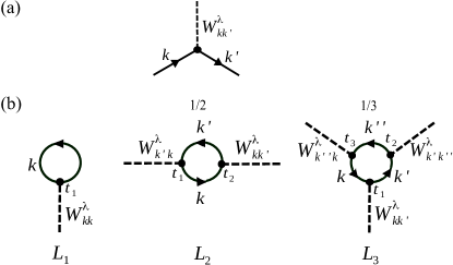
Figure 1: (a) Elementary interaction vertex. (b) First three connected diagrams $L_{1}$, $L_{2}$ and $L_{3}$ of the linked cluster expansion in the evaluation of the thermal average of the $S$-matrix $\braket{S(t,0)}$.

$$\begin{split}L_{1}(t)=&-\sum_{\lambda,\textbf{k}}\int_{0}^{t}\text{d}t_{1}W^{\lambda}_{\textbf{k},\textbf{k}}\,G^{0}_{\lambda\textbf{k}}(t_{1},t_{1}^{+})\\ L_{2}(t)=&-\frac{1}{2}\sum_{\lambda,\textbf{k},\textbf{k}^{\prime}}\Big{|}W^{\lambda}_{\textbf{k},\textbf{k}^{\prime}}\Big{|}^{2}\\ &\times\int_{0}^{t}\text{d}t_{1}\int_{0}^{t}\text{d}t_{2}\,G^{0}_{\lambda\textbf{k}}(t_{1},t_{2})\,G^{0}_{\lambda\textbf{k}^{\prime}}(t_{2},t_{1})\,,\end{split}$$ (14)

where $G^{0}_{\lambda\textbf{k}}$ is the free Green’s function for the WL state $\lambda\textbf{k}$.

For the first-order contribution one obtains an imaginary, linear time dependence, which amount to a correction to the exciton energy.

$$L_{1}(t)=-i\sum_{\lambda,\textbf{k}}W^{\lambda}_{\textbf{k},\textbf{k}}\,f^{\lambda}_{\textbf{k}}\,\,t$$ (15)

with $f^{\lambda}_{\textbf{k}}$ the Fermi function for the WL level carrying the same indices.

More important is the second order diagram ($\varepsilon^{\lambda}_{\textbf{k}\textbf{k}^{\prime}}$ denotes the difference $\varepsilon^{\lambda}_{\textbf{k}}-\varepsilon^{\lambda}_{\textbf{k}^{\prime}}$)

$$\begin{split}L_{2}(t)=&\sum_{\lambda,\textbf{k},\textbf{k}^{\prime}}\Big{|}W^{\lambda}_{\textbf{k},\textbf{k}^{\prime}}\Big{|}^{2}(1-f^{\lambda}_{\textbf{k}})f^{\lambda}_{\textbf{k}^{\prime}}\,\\ &\times\Big{(}e^{-i\,\varepsilon^{\lambda}_{\textbf{k}\textbf{k}^{\prime}}\,t}-1+i\,\varepsilon^{\lambda}_{\textbf{k}\textbf{k}^{\prime}}\,t\Big{)}\Big{(}\varepsilon^{\lambda}_{\textbf{k}\textbf{k}^{\prime}}\Big{)}^{-2}\,.\end{split}$$ (16)

Initially it decays quadratically with time, as obvious from the double integral from $0$ to $t$ in Eq.(14), and also reflected in Eq.(16) by the subtraction of the first two terms in the expansion of the exponential.

More relevant is the long-time behavior of the real part

$$\text{Re}L_{2}(t)=-\sum_{\lambda,\textbf{k},\textbf{k}^{\prime}}\Big{|}W^{\lambda}_{\textbf{k},\textbf{k}^{\prime}}\Big{|}^{2}(1-f^{\lambda}_{\textbf{k}})f^{\lambda}_{\textbf{k}^{\prime}}\,\,\frac{1-\cos(\varepsilon^{\lambda}_{\textbf{k}\textbf{k}^{\prime}}\,t)}{(\varepsilon^{\lambda}_{\textbf{k}\textbf{k}^{\prime}})^{2}}\,,$$ (17)

which controls the polarization decay. Indeed, using the large $t$ asymptotics of $(1-\cos\omega t)/\omega^{2}\sim\pi\,\delta(\omega)\,t$, one finds an exponential attenuation $\mathcal{P}(t)\sim\exp(-\Gamma t)$ with the decay rate given by

$$\Gamma=\pi\sum_{\lambda,\textbf{k},\textbf{k}^{\prime}}\Big{|}W^{\lambda}_{\textbf{k},\textbf{k}^{\prime}}\Big{|}^{2}(1-f^{\lambda}_{\textbf{k}})f^{\lambda}_{\textbf{k}^{\prime}}\,\delta(\varepsilon^{\lambda}_{\textbf{k}\textbf{k}^{\prime}})\,.$$ (18)

A comparative discussion with the IBM is in order. The dephasing process does not imply a change of population (pure dephasing) and therefore the decay rate $\Gamma$ does not involve energy transfer, as seen by the presence of the $\delta$-function. In the case of IBM that means only zero-energy phonons are involved. Then all the discussion takes place around the spectral edge, and depends on the density of states and coupling constants there. Usually they vanish as a higher power of energy and overcome the singularity of the Bose-Einstein distribution, with the result that $\Gamma=0$. This leads to the problem of the zero-phonon line (ZPL) appearing as an artificial pure $\delta$-peak in the spectrum. This is a weak point and several ways out have been devised, like including a phenomenological line broadening Zimmermann and Runge (2002), a phonon-phonon interaction Muljarov and Zimmermann (2004), or considering a lower dimensionality Lindwall et al. (2007) to enhance the density of states. The fermionic case is free from this problem, since $\Gamma$ relies on quantities around the chemical potential.

Also, it is worth noting that limiting the expansion to $L_{2}$ gives the exact result in the IBM, while here it is only an approximation. One may plead in favor of neglecting higher diagrams by arguing that a lot of compensation takes place between the direct terms in Eq.(3) and the exchange terms are small, in other words the QD-WL coupling is weak. Nevertheless, this is not sufficient, since it might turn out that higher order diagrams behave as higher powers in time, and thus asymptotically overtake the second order one. We argue below that this is not the case.

Indeed, the structure of the diagrams is such that the $\theta$-functions contained in the Green’s functions splits the expression into integrals of the form

$$I_{n}(t)=\int_{0}^{t}\text{d}t_{1}e^{i\omega_{1}t_{1}}\int_{0}^{t_{1}}\text{d}t_{2}e^{i\omega_{2}t_{2}}\,\ldots\int_{0}^{t_{n-1}}\text{d}t_{n}e^{i\omega_{n}t_{n}}\,.$$ (19)

The frequency appearing in each time integration is the difference of the energies of the Green’s functions meeting at the corresponding internal points. Summing these pairwise differences around the diagram entails the relation $\omega_{1}+\omega_{2}+\ldots+\omega_{n}=0$.

On the other hand, the Laplace transform of $I_{n}(t)$ can be easily calculated and gives

$$J_{n}(s)= \frac{1}{s}\,\frac{1}{s+i\omega_{1}}\,\frac{1}{s+i(\omega_{1}+\omega_{2})}\cdots$$

$$\cdots\frac{1}{s+i(\omega_{1}+\omega_{2}+\ldots+\omega_{n})}$$ (20)

The last factor is actually $1/s$, like the first, so that $J_{n}(s)\sim 1/s^{2}$ around $s=0$. This corresponds to a behavior $I_{n}(t)\sim t$ as $t\to\infty$ for all $n$. For instance, the $n=2$ case, discussed above, can be recovered from $J_{2}(s)=1/s^{2}\,\cdot 1/(s+i\omega_{1})$. The low-$s$ asymptotics of its real part generates the linear large time behavior times the $\pi\delta(\omega_{1})$ factor, with $\omega_{1}=\varepsilon^{\lambda}_{\textbf{k},\textbf{k}^{\prime}}$.

Using $g$ as a generic notation for the coupling strength, we conclude that the contribution of the diagram of order $n$ at large times is $\sim g^{n}\,t$. This is in agreement with the so-called weak interaction limit Spohn (1980), stating that when $g\to 0$ and simultaneously $t\to\infty$ so that $g^{2}\,t$ remains constant, the Born-Markov dissipative evolution becomes exact. Indeed, here all $n>2$ contributions vanish in this scaling limit.

III Numerical example

As an illustration we consider an InAs/GaAs heterostructure, with a self-assembled QD on a WL of $L=2.2$ nm width. The relevant material parameters are those of Vurgaftman et al. Vurgaftman et al. (2001). We assume the wavefunctions to be factorized into the square-well solution $\chi^{\lambda}(z)$ along the growth direction and the in-plane function. The latter are taken as oscillator ground-state gaussians for the QD $s$-states for electrons and holes, and as plane waves, orthogonalized on the former, for the WL extended states. The gaussians are defined by their width $\alpha_{\lambda}$ in the reciprocal space, i.e. $\varphi^{\lambda}_{s}(\textbf{r})=\alpha_{\lambda}/\sqrt{\pi}\exp(-\alpha^{2}_{\lambda}r^{2}/2)$ with r here the in-plane position. These parameters depend on many geometric and composition features of the QD, so that they can reach a broad set of values. For the sake of our example we take $\alpha_{e}=0.2/\text{nm}$ and $\alpha_{h}=0.1/\text{nm}$.

The phonon-induced dephasing is expected to be less important at low temperatures. The Coulomb-assisted dephasing depends on both temperature and WL-carrier concentration, therefore lowering the temperature and increasing the concentration it has a chance to compete with the phononic processes. We consider only the neutral charging, with electrons and holes in the WL at the same concentration $n$.

Figure 2: (color online) Time evolution of the real part of $\Phi$ for two temperatures, 5K (a) and 10K (b) at the same carrier concentration $n=10^{12}/\text{cm}^{2}$. The dephasing reaches a linear decay whose rate increases with temperature.

In Fig. 2 the time evolution of the real part of $\Phi(t)$ is plotted for two different temperatures. The inital quadratic behavior is followed by a linear decrease, whose slope $\Gamma$ is the dephasing rate predicted by Eq.(18). It increases with temperature, as confirmed by Fig. 3, which shows the values of $\Gamma$ at various temperatures and carrier concentrations.

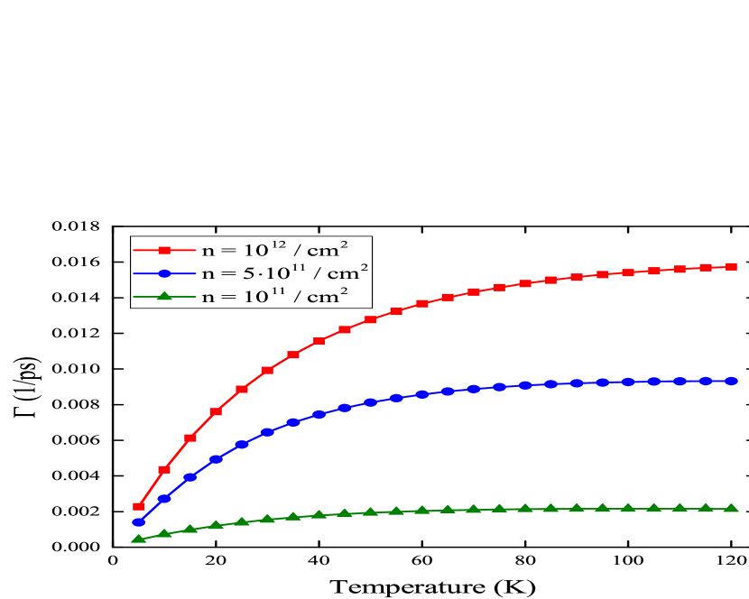
Figure 3: (color online) Dephasing rates $\Gamma$ as functions of temperature for different carrier concentrations.

The range of those values is such that $\hbar\Gamma$ is of the order of a few $\mu\text{eV}$. This is comparable with results for dephasing by phonons at low temperatures both in theoretical simulations Zimmermann and Runge (2002); Takagahara (1999) and in experimental data Borri et al. (2001, 2002). Experimental data obtained by four-wave mixing Borri et al. (2002) do not separate phonon and injected carrier contributions to dephasing, but their total effect is still in the $\mu\text{eV}$ range.

For an increase of temperatures from 5K to 120K the dephasing grows by roughly one order of magnitude. In the same conditions the rate of dephasing by phonons gains two orders of magnitude Zimmermann and Runge (2002); Borri et al. (2001), showing a higher sensitivity to temperature. Yet in the case of the fermionic bath the decay is enhanced also by increasing a second controllable parameter, the carrier concentration.

As mentioned above, the description of the phonon dephasing by the IBM runs into the ZPL problem. As seen in Refs. Li et al. (2014); Muljarov and Zimmermann (2004) the slope of the long-time linear asymptotics is zero, for reasons discussed Sec.II. This leads to an unphysical pure $\delta$-spike in the frequency domain.

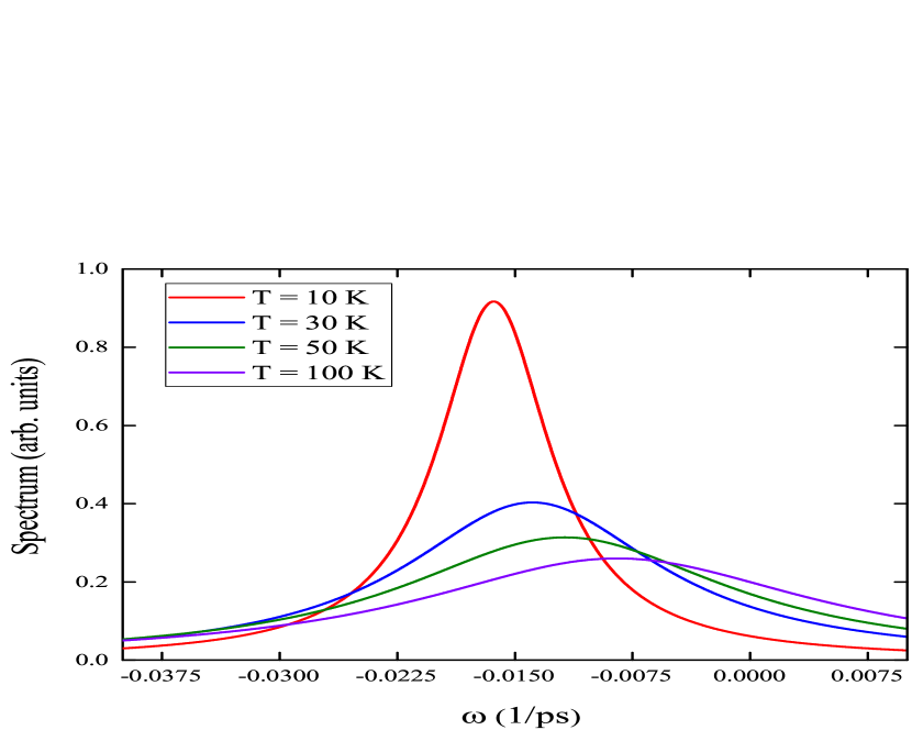
Figure 4: (color online) Absorption spectra for $n=10^{12}/\text{cm}^{2}$ at T=10, 30, 50, 100K

This is not the case with the fermionic bath, as also seen in Fig. 4. The main feature of the spectra is their Lorentzian shape, as a consequence of the exponential decay in the time domain. Still, the quadratic initial behavior replaces the cusp at $t=0$ of a pure exponential by a smooth matching. In the frequency domain this leads to a departure from the Lorentzian, in the sense of a faster decay at large frequencies.

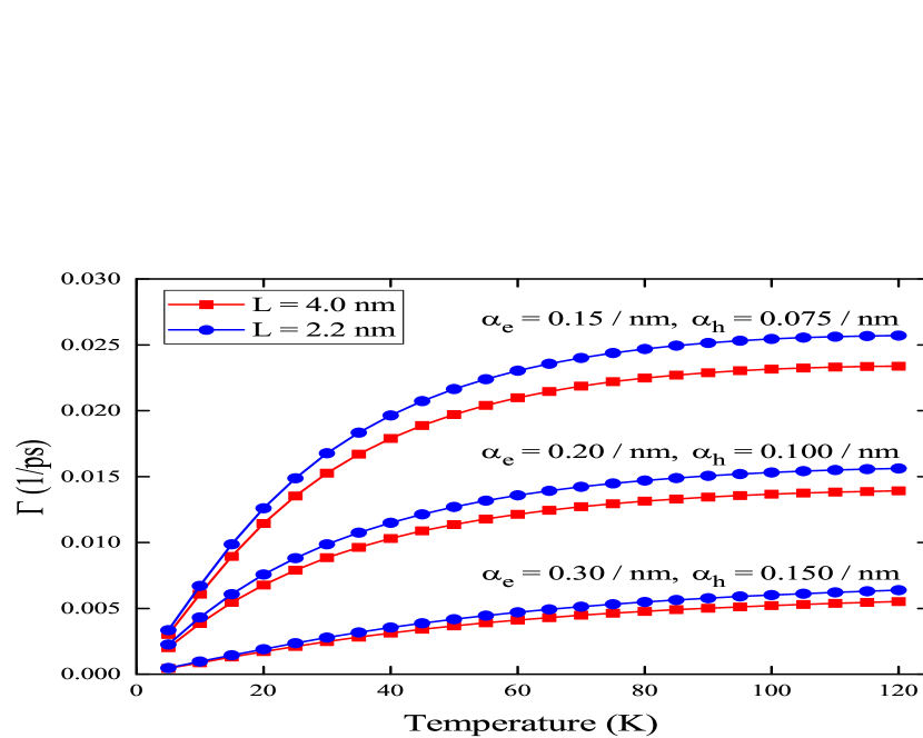
Figure 5: (color online) Temperature dependence of the dephasing rate for different WL width $L$ and space extension parameters $\alpha$. All curves for $n=10^{12}/\text{cm}^{2}$

In Fig. 5 we also consider the dependence of dephasing on other, more geometric parameters. It is seen that $\Gamma$ is not very sensitive to the WL width $L$, but it is significantly influenced by the spatial extension of the QD $s$-states. The broader the states, the stronger the dephasing, due to a more efficient scattering.

IV Conclusions

In conclusion, we have shown that a fermionic counterpart of the popular IBM is possible. It describes the QD exciton interaction with the fermionic bath consisting of injected carriers in the bulk or WL. Similarities and differences to the IBM are pointed out. For instance, the present solution takes the form of a diagrammatic series expansion, while the IBM is exact, but this advantage is lost as soon as other interactions are present. Also, our case is free from the ZPL problem inherent to the bosonic case. The dephasing process is controlled not only by temperature but also by the chemical potential of the bath. The numerical illustration shows that at low temperatures and higher carrier concentrations the dephasing times are comparable with those produced by the phonon interaction. But, of course, this is also dependent on the parameters of the particular case considered. The dephasing gets stronger at higher temperature and concentration, as well as with broader charge distribution of QD states.

References

- Mahan (2000) G. D. Mahan, Many Particle Physics (Springer, 2000), 3rd ed., ISBN 0306463385.
- Huang and Rhys (1950) K. Huang and A. Rhys, Proc. R. Soc. Ser. A 204, 406 (1950).
- Duke and Mahan (1965) C. B. Duke and G. D. Mahan, Phys. Rev. 139, A1965 (1965), URL https://link.aps.org/doi/10.1103/PhysRev.139.A1965.
- Zimmermann and Runge (2002) R. Zimmermann and E. Runge, in Proceedings of the 26th ICPS, Edinburgh, UK, edited by A. Long and J. Davies (IOP Publishing, Bristol, 2002), p. M 3.1.
- Lindwall et al. (2007) G. Lindwall, A. Wacker, C. Weber, and A. Knorr, Phys. Rev. Lett. 99, 087401 (2007), URL https://link.aps.org/doi/10.1103/PhysRevLett.99.087401.
- Li et al. (2014) X. Li, T. Wang, and C. Dong, IEEE J. Quantum Electron. 50, 548 (2014).
- Dusanowski et al. (2014) L. Dusanowski, A. Musiał, A. Maryński, P. Mrowiński, J. Andrzejewski, P. Machnikowski, J. Misiewicz, A. Somers, S. Höfling, J. P. Reithmaier, et al., Phys. Rev. B 90, 125424 (2014), URL https://link.aps.org/doi/10.1103/PhysRevB.90.125424.
- Florian et al. (2013) M. Florian, P. Gartner, C. Gies, and F. Jahnke, New J. Phys. 15, 035019 (2013).
- Hohenester (2010) U. Hohenester, Phys. Rev. B 81, 155303 (2010), URL https://link.aps.org/doi/10.1103/PhysRevB.81.155303.
- Hahn et al. (2019) T. Hahn, D. Groll, T. Kuhn, and D. Wigger, Phys. Rev. B 100, 024306 (2019), URL https://link.aps.org/doi/10.1103/PhysRevB.100.024306.
- Sengupta (2019) S. Sengupta, Phys. Rev. B 100, 075429 (2019), URL https://link.aps.org/doi/10.1103/PhysRevB.100.075429.
- Besombes et al. (2001) L. Besombes, K. Kheng, L. Marsal, and H. Mariette, Phys. Rev. B 63, 155307 (2001), URL https://link.aps.org/doi/10.1103/PhysRevB.63.155307.
- Taylor (2006) J. R. Taylor, Scattering Theory (Dover Publications, N.Y., 2006).
- Sitenko (1991) A. G. Sitenko, Scattering Theory (Springer, 1991), ISBN 3642840361.
- Florian et al. (2014) M. Florian, P. Gartner, A. Steinhoff, C. Gies, and F. Jahnke, Phys. Rev. B 89, 161302 (2014), URL https://link.aps.org/doi/10.1103/PhysRevB.89.161302.
- Abrikosov (1975) A. A. Abrikosov, Methods of Quantum Field Theory in Statistical Physics (Dover Publications, N.Y., 1975), revised ed., ISBN 0486632288.
- Muljarov and Zimmermann (2004) E. A. Muljarov and R. Zimmermann, Phys. Rev. Lett. 93, 237401 (2004), URL https://link.aps.org/doi/10.1103/PhysRevLett.93.237401.
- Spohn (1980) H. Spohn, Rev. Mod. Phys. 52, 569 (1980), URL https://link.aps.org/doi/10.1103/RevModPhys.52.569.
- Vurgaftman et al. (2001) I. Vurgaftman, J. R. Meyer, and L. R. Ram-Mohan, Appl. Phys. Rev. 89, 5815 (2001), URL https://doi.org/10.1063/1.1368156.
- Takagahara (1999) T. Takagahara, Phys. Rev. B 60, 2638 (1999), URL https://link.aps.org/doi/10.1103/PhysRevB.60.2638.
- Borri et al. (2001) P. Borri, W. Langbein, S. Schneider, U. Woggon, R. L. Sellin, D. Ouyang, and D. Bimberg, Phys. Rev. Lett. 87, 157401 (2001), URL https://link.aps.org/doi/10.1103/PhysRevLett.87.157401.
- Borri et al. (2002) P. Borri, W. Langbein, S. Schneider, U. Woggon, R. L. Sellin, D. Ouyang, and D. Bimberg, Phys. Rev. Lett. 89, 187401 (2002), URL https://link.aps.org/doi/10.1103/PhysRevLett.89.187401.