Trading Convergence Rate with Computational Budget in High Dimensional Bayesian Optimization


Hung Tran-The, Sunil Gupta, Santu Rana, Svetha Venkatesh
Applied Artificial Intelligence Institute,Deakin University, Geelong, Australia
{hung.tranthe, sunil.gupta, santu.rana, svetha.venkatesh}@deakin.edu.au
Abstract

Scaling Bayesian optimisation (BO) to high-dimensional search spaces is a active and open research problems particularly when no assumptions are made on function structure. The main reason is that at each iteration, BO requires to find global maximisation of acquisition function, which itself is a non-convex optimization problem in the original search space. With growing dimensions, the computational budget for this maximisation gets increasingly short leading to inaccurate solution of the maximisation. This inaccuracy adversely affects both the convergence and the efficiency of BO. We propose a novel approach where the acquisition function only requires maximisation on a discrete set of low dimensional subspaces embedded in the original high-dimensional search space. Our method is free of any low dimensional structure assumption on the function unlike many recent high-dimensional BO methods. Optimising acquisition function in low dimensional subspaces allows our method to obtain accurate solutions within limited computational budget. We show that in spite of this convenience, our algorithm remains convergent. In particular, cumulative regret of our algorithm only grows sub-linearly with the number of iterations. More importantly, as evident from our regret bounds, our algorithm provides a way to trade the convergence rate with the number of subspaces used in the optimisation. Finally, when the number of subspaces is โ€sufficiently largeโ€, our algorithmโ€™s cumulative regret is at most ๐’ชโˆ—โ€‹(Tโ€‹ฮณT)superscript๐’ช๐‘‡subscript๐›พ๐‘‡\mathcal{O}^{*}(\sqrt{T\gamma_{T}}) as opposed to ๐’ชโˆ—โ€‹(Dโ€‹Tโ€‹ฮณT)superscript๐’ช๐ท๐‘‡subscript๐›พ๐‘‡\mathcal{O}^{*}(\sqrt{DT\gamma_{T}}) for the GP-UCB of Srinivas et al. (2012), reducing a crucial factor D๐ท\sqrt{D} where D๐ทD being the dimensional number of input space. We perform empirical experiments to evaluate our method extensively, showing that its sample efficiency is better than the existing methods for many optimisation problems involving dimensions up to 5000.

Introduction

Bayesian optimization (BO) offers an efficient solution to find the global optimum of expensive black-box functions, a problem that is all pervasive in real-world experimental design applications. However, the scalability of BO is particularly compromised in high dimensions (>15absent15>15 dimensions).

The main difficulty that a BO algorithm faces in high dimensions is that at each iteration, it needs to find the global maximum of a surrogate function called the acquisition function in order to suggest the next function evaluation point. The acquisition function balances two conflicting requirements: evaluating the function at a location where the function may peak as indicated by knowledge collected so far (exploitation) and evaluating the function at a location to reduce our uncertaiity about the function (exploration). The acquisition function itself is a non-convex optimisation problem in the original search space. With growing dimensions, any fixed computational budget for this optimisation becomes quickly insufficient leading to inaccurate solutions. This inaccuracy adversely affects both the convergence and the efficiency of the BO algorithm.

In order to make the problem scalable, most of the current methods make restrictive structural assumptions such as the function having an effective low-dimensional subspace (?;ย ?;ย ?;ย ?;ย ?;ย ?), or being decomposable in subsets of dimensions (?;ย ?;ย ?;ย ?;ย ?). Through these assumptions, the acquisition function becomes easier to optimise and the global optimum can be found. However, such assumptions are rather strong and since we are dealing with unknown function, we have no way of knowing if such assumptions hold in reality.

Without these assumptions, the high-dimensional BO problem is more challenging. There have been some recent attempts to develop scalable BO methods. For example, (?) use an elastic Gaussian process model to reduce the โ€flatnessโ€ of the acquistion function in high dimensions and thus improve the solution. Although this method helps obtains improved optimum of the acquistion function, it still does not provide any way to scale BO to high dimensions. (?) devise a method under the assumption that the solution does not lie at the boundary of the search space and thus drive the BO search towards the interior of the search space using polar co-ordinate transformations. Thus, the convergence analysis of (?) depends on whether their assumptions holds. Some other methods are based on subspaces (?;ย ?;ย ?), which are more amenable to convergence analysis. Among them, LineBO (?) is the first to provide a complete analysis. In LineBO, the maximisation of the acquisition function is performed on a one-dimensional random subspace. Although this solution is computationally effective, the regret bound of LineBO does not scale well with the search space dimension and gets increasingly worse compared to the regret of the GP-UCB (?). Thus we still need a method that is both computationally efficient and offers optimal sample efficiency in high dimensions in a flexible manner.

We propose a novel algorithm for high-dimensional BO without making any restrictive assumptions on the function structure and show that our algorithm attains better regret than previous methods. The key insight of our method is that instead of maximizing the acquisition function on the full search space that is computationally prohibitive in high dimensions, we will maximize it on a restricted space that consist of multiple low-dimensional subspaces. This approach has several benefits. If the acquisition function is maximised in low-dimensional subspaces then computations involved in finding the solution of acquisition function optimisation are practically feasible while multiple subspaces can still cover the search space well if they are chosen in a principled manner. Further, this method allows us to theoretically derive a cumulative regret as a function of the number of subspaces. The crucial advantage is that we can trade between the computations and the convergence rate of the algorithm while still maintaining efficient convergence (i.e. a sublinear growth of cumulative regret). Our contributions in this paper are:

  • โ€ข

    A novel BO algorithm based on multiple random subspaces that offers the flexibility to trade between the computations and the convergence rate. To do this, we propose to decompose the original search space into multiple lower-dimensional spaces via a randomisation technique.

  • โ€ข

    We derive an upper bound on the cumulative regret for our algorithm and theoretically show that it has a sublinear growth rate and further, larger the number of subspaces, tighter the cumulative regret. Further, when the number of subspaces is large enough, the cumulative regret is at most of order ๐’ชโˆ—โ€‹(Tโ€‹ฮณT)superscript๐’ช๐‘‡subscript๐›พ๐‘‡\mathcal{O}^{*}(\sqrt{T\gamma_{T}}) as opposed to the regret bound of GP-UCB ๐’ชโˆ—โ€‹(Dโ€‹Tโ€‹ฮณT)superscript๐’ช๐ท๐‘‡subscript๐›พ๐‘‡\mathcal{O}^{*}(\sqrt{DT\gamma_{T}}). The regret bound of our algorithm is tighter by a factor of D๐ท\sqrt{D}. In some situations (detailed in the paper), this improvement is possible with fewer computations than GP-UCB - a double advantage.

  • โ€ข

    We also study a special case when the objective function has an effective low dimensional subspace as assumed by many previous methods e.g. REMBO (?). We show that our algorithm automatically benefits from this low dimensional structure with the tighter bound.

  • โ€ข

    We extensively evaluate our method using a variety of optimisation tasks including optimisation of several benchmark functions as well as learning the parameters of a moderately sized neural network and a classification model based on non-convex ramp loss. We compare our method with several existing high dimensional BO algorithms and demonstrate that given equal computational budget, the sample efficiency of our method is consistently better than that of the existing methods.

Preliminaries

We consider the global maximization problem of the form

๐ฑโˆ—=argmax๐ฑโˆˆ๐’ณโ€‹fโ€‹(๐ฑ)superscript๐ฑsubscriptargmax๐ฑ๐’ณ๐‘“๐ฑ\displaystyle\mathbf{x}^{*}=\text{argmax}_{\mathbf{x}\in\mathcal{X}}f(\mathbf{x}) (1)

in a compact search space ๐’ณ=[โˆ’1,1]D๐’ณsuperscript11๐ท\mathcal{X}=[-1,1]^{D}. In this paper we are especially concerned about problems with high values of D๐ทD. We consider functions f๐‘“f that are blackbox and expensive to evaluate, and our goal is to find the optimum in a minimal number of samples. We further assume we only have access to noisy evaluations of f๐‘“f in the form u=fโ€‹(๐ฑ)+ฯต๐‘ข๐‘“๐ฑitalic-ฯตu=f(\mathbf{x})+\epsilon where the noise ฯตโˆผ๐’ฉโ€‹(0,ฯƒ2)similar-toitalic-ฯต๐’ฉ0superscript๐œŽ2\epsilon\sim\mathcal{N}(0,\sigma^{2}) is i.i.d. Gaussian.

Bayesian Optimization

BO offers a principal framework to approach the global optimisation problem. The standard BO routine consists of two key steps: estimating the black-box function from function evaluation data and maximizing an acquisition function to suggest next function evaluation point balancing exploration and exploitation. Gaussian process (GP) (?) is a popular choice for the first step due to its tractability for posterior and predictive distributions: fโ€‹(๐ฑ)=๐’ขโ€‹๐’ซโ€‹(mโ€‹(๐ฑ),kโ€‹(๐ฑ,๐ฑโ€ฒ))๐‘“๐ฑ๐’ข๐’ซ๐‘š๐ฑ๐‘˜๐ฑsuperscript๐ฑโ€ฒf(\mathbf{x})=\mathcal{GP}(m(\mathbf{x}),k(\mathbf{x},\mathbf{x}^{\prime})), where mโ€‹(๐ฑ)๐‘š๐ฑm(\mathbf{x}) and kโ€‹(๐ฑ,๐ฑโ€ฒ)๐‘˜๐ฑsuperscript๐ฑโ€ฒk(\mathbf{x},\mathbf{x}^{\prime}) are the mean and the covariance (or kernel) functions. Popular covariance functions include linear kernel, squared exponential (SE) kernel, Matern kernel etc. The predictive mean and variance of Gaussian process is a Gaussian distribution. Given a set of observations ๐’Ÿ1:t={๐ฑi,ui}i=1tsubscript๐’Ÿ:1๐‘กsuperscriptsubscriptsubscript๐ฑ๐‘–subscript๐‘ข๐‘–๐‘–1๐‘ก\mathcal{D}_{1:t}=\{\mathbf{x}_{i},u_{i}\}_{i=1}^{t}, the predictive distribution can be derived as: Pโ€‹(ft+1|๐’Ÿ1:t,๐ฑ)=๐’ฉโ€‹(ฮผt+1โ€‹(๐ฑ),ฯƒt+12โ€‹(๐ฑ))๐‘ƒconditionalsubscript๐‘“๐‘ก1subscript๐’Ÿ:1๐‘ก๐ฑ๐’ฉsubscript๐œ‡๐‘ก1๐ฑsuperscriptsubscript๐œŽ๐‘ก12๐ฑP(f_{t+1}|\mathcal{D}_{1:t},\mathbf{x})=\mathcal{N}(\mu_{t+1}(\mathbf{x}),\sigma_{t+1}^{2}(\mathbf{x})), where ฮผt+1โ€‹(๐ฑ)=kTโ€‹[๐Š+ฯƒ2โ€‹I]โˆ’1โ€‹u+mโ€‹(๐ฑ)subscript๐œ‡๐‘ก1๐ฑsuperscriptk๐‘‡superscriptdelimited-[]๐Šsuperscript๐œŽ2I1u๐‘š๐ฑ\mu_{t+1}(\mathbf{x})=\textbf{k}^{T}[\mathbf{K}+\sigma^{2}\textbf{I}]^{-1}\textbf{u}+m(\mathbf{x}) and ฯƒt+12โ€‹(๐ฑ)=kโ€‹(๐ฑ,x)โˆ’kTโ€‹[K+ฯƒ2โ€‹I]โˆ’1โ€‹ksuperscriptsubscript๐œŽ๐‘ก12๐ฑ๐‘˜๐ฑxsuperscriptk๐‘‡superscriptdelimited-[]Ksuperscript๐œŽ2I1k\sigma_{t+1}^{2}(\mathbf{x})=k(\mathbf{x},\textbf{x})-\text{{k}}^{T}[\textbf{K}+\sigma^{2}\textbf{I}]^{-1}\textbf{k}. In the above expression we define kย =[kโ€‹(๐ฑ,๐ฑ1),โ€ฆ,kโ€‹(๐ฑ,๐ฑt)]kย ๐‘˜๐ฑsubscript๐ฑ1โ€ฆ๐‘˜๐ฑsubscript๐ฑ๐‘ก\textbf{k }=[k(\mathbf{x},\mathbf{x}_{1}),...,k(\mathbf{x},\mathbf{x}_{t})], Kย =[kโ€‹(๐ฑi,๐ฑj)]1โ‰คi,jโ‰คtKย subscriptdelimited-[]๐‘˜subscript๐ฑ๐‘–subscript๐ฑ๐‘—formulae-sequence1๐‘–๐‘—๐‘ก\textbf{K }=[k(\mathbf{x}_{i},\mathbf{x}_{j})]_{1\leq i,j\leq t} and u=[u1,โ€ฆ,ut]usubscript๐‘ข1โ€ฆsubscript๐‘ข๐‘ก\textbf{u}=[u_{1},\ldots,u_{t}].

The acquisition functions are designed to trade off between exploration of the search space and exploitation of current promising region. Some examples of acquisition functions include Expected Improvement (EI) (?) and GP-UCB (?). A GP-UCB acquisition function at iteration t+1๐‘ก1t+1 is defined as

at+1โ€‹(๐ฑ)=ฮผtโ€‹(๐ฑ)+ฮฒt+1โ€‹ฯƒtโ€‹(๐ฑ)subscript๐‘Ž๐‘ก1๐ฑsubscript๐œ‡๐‘ก๐ฑsubscript๐›ฝ๐‘ก1subscript๐œŽ๐‘ก๐ฑ\displaystyle a_{t+1}(\mathbf{x})=\mu_{t}(\mathbf{x})+\sqrt{\beta_{t+1}}\sigma_{t}(\mathbf{x}) (2)

where ฮฒt+1subscript๐›ฝ๐‘ก1\beta_{t+1} is a parameter to balance exploration and exploitation. There are guidelines (?) for setting ฮฒt+1subscript๐›ฝ๐‘ก1\beta_{t+1} to achieve sublinear regret.

Proposed Method

To solve the Bayesian optimization problem in high dimensions, the main difficulty is the prohibitive computational burden when maximising the acquisition function which requires solving a non-convex optimization problem in the same search space. Working with a small computational budget usually directly affects the quality of the point suggested by the acquisition step and consequently, many BO algorithms that require finding exactly the maximisers of the acquisition function (e.g. EI, GP-UCB) perform poorly in high dimensions. We propose a novel approach for this problem as follows. Instead of maximising the acquisition function on the whole space, we perform it only on a discrete set of low-dimensional subspaces generated by random sampling. This approach brings several benefits. First, it solves the computation challenge effectively. Second, it provides a way to trade between the computations and the sample efficiency for convergence. Finally, our analysis suggests that when the number of subspaces are sufficiently high, our approach can simultaneously offer both lower computational requirement and better sample efficiency.

Before introducing our method, we formally define the low dimensional subspaces (see Definition 1) that will be used in our method.

Subspace Description

Lemma 1.

Given a dโˆˆ{1,โ€ฆ,Dโˆ’1}๐‘‘1โ€ฆ๐ท1d\in\{1,...,D-1\}, for any xโˆˆ[โˆ’1,1]D๐‘ฅsuperscript11๐ทx\in[-1,1]^{D}, there exists a yโˆˆ[โˆ’1,1]d๐‘ฆsuperscript11๐‘‘y\in[-1,1]^{d} and a zโˆˆ[โˆ’1,1]Dโˆ’d๐‘งsuperscript11๐ท๐‘‘z\in[-1,1]^{D-d} such that

๐ฑ=๐€๐ฒ+๐๐ณ๐ฑ๐€๐ฒ๐๐ณ\mathbf{x}=\mathbf{A}\mathbf{y}+\mathbf{B}\mathbf{z}

where matrix ๐€=[๐ŸŽdร—(Dโˆ’d),๐ˆdร—d]T๐€superscriptsuperscript0๐‘‘๐ท๐‘‘superscript๐ˆ๐‘‘๐‘‘๐‘‡\mathbf{A}=[\mathbf{0}^{d\times(D-d)},\mathbf{I}^{d\times d}]^{T} and matrix ๐=[๐ˆ(Dโˆ’d)ร—(Dโˆ’d),๐ŸŽ(Dโˆ’d)ร—d]T๐superscriptsuperscript๐ˆ๐ท๐‘‘๐ท๐‘‘superscript0๐ท๐‘‘๐‘‘๐‘‡\mathbf{B}=[\mathbf{I}^{(D-d)\times(D-d)},\mathbf{0}^{(D-d)\times d}]^{T}.

Proof.

Given any ๐ฑโˆˆ๐’ณ๐ฑ๐’ณ\mathbf{x}\in\mathcal{X}, we denote the first Dโˆ’d๐ท๐‘‘D-d elements of vector ๐ฑ๐ฑ\mathbf{x} by [๐ฑ]1:Dโˆ’dsubscriptdelimited-[]๐ฑ:1๐ท๐‘‘[\mathbf{x}]_{1:D-d} and the last d๐‘‘d elements of vector ๐ฑ๐ฑ\mathbf{x} by [๐ฑ]Dโˆ’d+1:Dsubscriptdelimited-[]๐ฑ:๐ท๐‘‘1๐ท[\mathbf{x}]_{D-d+1:D}. We set ๐ฒ=[๐ฑ]Dโˆ’d+1:Dโˆˆ[โˆ’1,1]d๐ฒsubscriptdelimited-[]๐ฑ:๐ท๐‘‘1๐ทsuperscript11๐‘‘\mathbf{y}=[\mathbf{x}]_{D-d+1:D}\in[-1,1]^{d} and z=[๐ฑ]1:Dโˆ’dโˆˆ[โˆ’1,1]Dโˆ’d๐‘งsubscriptdelimited-[]๐ฑ:1๐ท๐‘‘superscript11๐ท๐‘‘z=[\mathbf{x}]_{1:D-d}\in[-1,1]^{D-d}. Thus, we have ๐ฑ=๐€๐ฒ+๐๐ณ๐ฑ๐€๐ฒ๐๐ณ\mathbf{x}=\mathbf{A}\mathbf{y}+\mathbf{B}\mathbf{z} with ๐ฒโˆˆ[โˆ’1,1]d๐ฒsuperscript11๐‘‘\mathbf{y}\in[-1,1]^{d} and ๐ณโˆˆ[โˆ’1,1]Dโˆ’d๐ณsuperscript11๐ท๐‘‘\mathbf{z}\in[-1,1]^{D-d}. โˆŽ

The main idea is that we split the dimensions of any point x๐‘ฅx in D๐ทD dimensional space into two groups: the first Dโˆ’d๐ท๐‘‘D-d dimensions correspond to z๐‘งz and the last d๐‘‘d dimensions correspond to y๐‘ฆy. Next, we define a set of subspaces based on this idea in the following form:

Definition 1 (Embedding Subspace).

Given a dโˆˆ{1,โ€ฆ,Dโˆ’1}๐‘‘1โ€ฆ๐ท1d\in\{1,...,D-1\} and a vector ๐ณโˆˆ๐’ต=[โˆ’1,1]Dโˆ’d๐ณ๐’ตsuperscript11๐ท๐‘‘\mathbf{z}\in\mathcal{Z}=[-1,1]^{D-d}. We define an embedding subspace ๐’ฎโ€‹(๐€,๐ณ)๐’ฎ๐€๐ณ\mathcal{S}(\mathbf{A},\mathbf{z}) as

๐’ฎโ€‹(๐€,๐ณ)={๐€๐ฒ+๐๐ณ|๐ฒโˆˆ๐’ด=[โˆ’1,1]d}๐’ฎ๐€๐ณconditional-set๐€๐ฒ๐๐ณ๐ฒ๐’ดsuperscript11๐‘‘\displaystyle\mathcal{S}(\mathbf{A},\mathbf{z})=\{\mathbf{A}\mathbf{y}+\mathbf{B}\mathbf{z}|\mathbf{y}\in\mathcal{Y}=[-1,1]^{d}\} (3)

where matrix ๐€=[๐ŸŽdร—(Dโˆ’d),๐ˆdร—d]T๐€superscriptsuperscript0๐‘‘๐ท๐‘‘superscript๐ˆ๐‘‘๐‘‘๐‘‡\mathbf{A}=[\mathbf{0}^{d\times(D-d)},\mathbf{I}^{d\times d}]^{T} and matrix ๐=[๐ˆ(Dโˆ’d)ร—(Dโˆ’d),๐ŸŽ(Dโˆ’d)ร—d]T๐superscriptsuperscript๐ˆ๐ท๐‘‘๐ท๐‘‘superscript0๐ท๐‘‘๐‘‘๐‘‡\mathbf{B}=[\mathbf{I}^{(D-d)\times(D-d)},\mathbf{0}^{(D-d)\times d}]^{T}.

The Proposed Algorithm

Our algorithm (presented in Algorithm 1) closely follows the standard BO algorithm. The main difference lies in the acquisition step that guides the selection of the next function evaluation point. We refer to our algorithm as MS-UCB.

Lemma 1 implies that there exists a ๐ฒโˆ—โˆˆ[โˆ’1,1]dsuperscript๐ฒsuperscript11๐‘‘\mathbf{y}^{*}\in[-1,1]^{d} and ๐ณโˆ—โˆˆ[โˆ’1,1]Dโˆ’dsuperscript๐ณsuperscript11๐ท๐‘‘\mathbf{z}^{*}\in[-1,1]^{D-d} such that

๐ฑโˆ—=๐€๐ฒโˆ—+๐๐ณโˆ—superscript๐ฑsuperscript๐€๐ฒsuperscript๐๐ณ\displaystyle\mathbf{x}^{*}=\mathbf{A}\mathbf{y}^{*}+\mathbf{B}\mathbf{z}^{*} (4)

Therefore, we can preserve any optimum point ๐ฑโˆ—superscript๐ฑ\mathbf{x}^{*} in the original space via ๐ฒโˆ—,๐ณโˆ—superscript๐ฒsuperscript๐ณ\mathbf{y}^{*},\mathbf{z}^{*} in two lower-dimensional spaces (via dimension splitting). This observation gives rise to our new idea that instead of optimising f๐‘“f on the original space, we can perform it in the lower dimensional spaces ๐’ด๐’ด\mathcal{Y} and ๐’ต๐’ต\mathcal{Z}:

๐ฒโˆ—,๐ณโˆ—=argmax๐ฒโˆˆ๐’ด,๐ณโˆˆ๐’ตโ€‹fโ€‹(๐€๐ฒ+๐๐ณ)superscript๐ฒsuperscript๐ณsubscriptargmaxformulae-sequence๐ฒ๐’ด๐ณ๐’ต๐‘“๐€๐ฒ๐๐ณ\displaystyle\mathbf{y}^{*},\mathbf{z}^{*}=\text{argmax}_{\mathbf{y}\in\mathcal{Y},\mathbf{z}\in\mathcal{Z}}f(\mathbf{A}\mathbf{y}+\mathbf{B}\mathbf{z}) (5)

where we denote the range [โˆ’1,1]dsuperscript11๐‘‘[-1,1]^{d} by ๐’ด๐’ด\mathcal{Y} and the range [โˆ’1,1]Dโˆ’dsuperscript11๐ท๐‘‘[-1,1]^{D-d} by ๐’ต๐’ต\mathcal{Z}. Note that this is different from (?;ย ?) where they assume an effective subspace on f๐‘“f. In that case, using a low-dimensional subspace can solve the BO problem. In our problem without any restrictive assumption on f๐‘“f, we need to use two low-dimensional subspaces to preserve an optimum. As a result, when Eq (27) is established, maximising the acquisition function atsubscript๐‘Ž๐‘กa_{t} will be performed in spaces ๐’ด๐’ด\mathcal{Y} and ๐’ต๐’ต\mathcal{Z} as

๐ฒt,๐ณt=argmax๐ฒโˆˆ๐’ด,๐ณโˆˆ๐’ตโ€‹atโ€‹(๐€๐ฒ+๐๐ณ)subscript๐ฒ๐‘กsubscript๐ณ๐‘กsubscriptargmaxformulae-sequence๐ฒ๐’ด๐ณ๐’ตsubscript๐‘Ž๐‘ก๐€๐ฒ๐๐ณ\displaystyle\mathbf{y}_{t},\mathbf{z}_{t}=\text{argmax}_{\mathbf{y}\in\mathcal{Y},\mathbf{z}\in\mathcal{Z}}a_{t}(\mathbf{A}\mathbf{y}+\mathbf{B}\mathbf{z}) (6)

In high dimensions where we may set d<<Dmuch-less-than๐‘‘๐ทd<<D, the (Dโˆ’d)๐ท๐‘‘(D-d)-dimensional space ๐’ต๐’ต\mathcal{Z} would itself be a high-dimensional space. Therefore, maximising the acquisition function in this space is still computationally expensive. To deal with this problem, we work with a finite set of samples ๐ณโˆˆ๐’ต๐ณ๐’ต\mathbf{z}\in\mathcal{Z} and maximise the acquisition function only on this finite set instead of the whole space ๐’ต๐’ต\mathcal{Z}. Let Ztsubscript๐‘๐‘กZ_{t} be the set of all ๐ณ๐ณ\mathbf{z} generated up to iteration t๐‘กt. With this modification, our acquisition step becomes:

๐ฒt,๐ณt=argmax๐ฒโˆˆ๐’ด,๐ณโˆˆ๐’ตtโ€‹atโ€‹(๐€๐ฒ+๐๐ณ)subscript๐ฒ๐‘กsubscript๐ณ๐‘กsubscriptargmaxformulae-sequence๐ฒ๐’ด๐ณsubscript๐’ต๐‘กsubscript๐‘Ž๐‘ก๐€๐ฒ๐๐ณ\displaystyle\mathbf{y}_{t},\mathbf{z}_{t}=\text{argmax}_{\mathbf{y}\in\mathcal{Y},\mathbf{z}\in\mathcal{Z}_{t}}a_{t}(\mathbf{A}\mathbf{y}+\mathbf{B}\mathbf{z}) (7)

Once ๐ณ๐ณ\mathbf{z} is sampled, a subspace ๐’ฎโ€‹(๐€,๐ณ)๐’ฎ๐€๐ณ\mathcal{S}(\mathbf{A},\mathbf{z}) as in Definition 1 is generated. Let ๐’ณtโ‰œ{๐’ฎโ€‹(๐€,๐ณi)โˆฃ๐ณiโˆˆZt}โ‰œsubscript๐’ณ๐‘กconditional-set๐’ฎ๐€superscript๐ณ๐‘–superscript๐ณ๐‘–subscript๐‘๐‘ก\mathcal{X}_{t}\triangleq\{\mathcal{S}(\mathbf{A},\mathbf{z}^{i})\mid\mathbf{z}^{i}\in Z_{t}\}. The Eq (7) can then be re-written as

๐ฑt=argmax๐ฑโˆˆ๐’ณtโ€‹atโ€‹(๐ฑ)subscript๐ฑ๐‘กsubscriptargmax๐ฑsubscript๐’ณ๐‘กsubscript๐‘Ž๐‘ก๐ฑ\displaystyle\mathbf{x}_{t}=\text{argmax}_{\mathbf{x}\in\mathcal{X}_{t}}a_{t}(\mathbf{x}) (8)

By Definition 1, we can see that for any subspace ๐’ฎโ€‹(๐€,๐ณi)๐’ฎ๐€superscript๐ณ๐‘–\mathcal{S}(\mathbf{A},\mathbf{z}^{i}), ๐’ฎโ€‹(๐€,๐ณi)โŠ‚๐’ณ๐’ฎ๐€superscript๐ณ๐‘–๐’ณ\mathcal{S}(\mathbf{A},\mathbf{z}^{i})\subset\mathcal{X}. Thus, the suggested point xtsubscript๐‘ฅ๐‘กx_{t} is always within ๐’ณ๐’ณ\mathcal{X}. This is a benefit of our dimension splitting based subspace projection as opposed to complex corrections required for previous methods ((?;ย ?)). We note that for our method atโ€‹(๐ฑ)=ฮผtโˆ’1โ€‹(๐ฑ)+ฮฒtโ€‹ฯƒtโˆ’1โ€‹(๐ฑ)subscript๐‘Ž๐‘ก๐ฑsubscript๐œ‡๐‘ก1๐ฑsubscript๐›ฝ๐‘กsubscript๐œŽ๐‘ก1๐ฑa_{t}(\mathbf{x})=\mu_{t-1}(\mathbf{x})+\sqrt{\beta_{t}}\sigma_{t-1}(\mathbf{x}) where ฮฒt=2โ€‹lโ€‹oโ€‹gโ€‹(ฯ€2โ€‹t2ฮด)+2โ€‹dโ€‹lโ€‹oโ€‹gโ€‹(2โ€‹bโ€‹dโ€‹lโ€‹oโ€‹gโ€‹(6โ€‹Dโ€‹aฮด)โ€‹t2)subscript๐›ฝ๐‘ก2๐‘™๐‘œ๐‘”superscript๐œ‹2superscript๐‘ก2๐›ฟ2๐‘‘๐‘™๐‘œ๐‘”2๐‘๐‘‘๐‘™๐‘œ๐‘”6๐ท๐‘Ž๐›ฟsuperscript๐‘ก2\beta_{t}=2log(\frac{\pi^{2}t^{2}}{\delta})+2dlog(2bd\sqrt{log(\frac{6Da}{\delta})}t^{2}). The ฮฒtsubscript๐›ฝ๐‘ก\beta_{t} of GP-UCB depends linearly on D๐ทD whereas the dependence of our ฮฒtsubscript๐›ฝ๐‘ก\beta_{t} on D๐ทD is only logโ€‹Dlog๐ท\sqrt{\text{log}D}.

A simple way to maximise atsubscript๐‘Ž๐‘กa_{t} on ๐’ณtsubscript๐’ณ๐‘ก\mathcal{X}_{t} is to maximise atsubscript๐‘Ž๐‘กa_{t} on each subspace ๐’ฎโ€‹(๐€,๐ณti)๐’ฎ๐€subscriptsuperscript๐ณ๐‘–๐‘ก\mathcal{S}(\mathbf{A},\mathbf{z}^{i}_{t}) separately and thus the returned value ๐ฑtsubscript๐ฑ๐‘ก\mathbf{x}_{t} is the maximizer on the all subspaces at iteration t๐‘กt. For a small d๐‘‘d, ๐’ฎโ€‹(๐€,๐ณi)๐’ฎ๐€superscript๐ณ๐‘–\mathcal{S}(\mathbf{A},\mathbf{z}^{i}) is a low-dimensional subspace of ๐’ณ๐’ณ\mathcal{X}. Thus, maximizing the acquisition function on such a subspace is computationally cheaper.

Importantly, we can show that maximising atsubscript๐‘Ž๐‘กa_{t} on a discrete set of subspaces can result in low regret by proposing a strategy to choose set Ztsubscript๐‘๐‘กZ_{t}. At iteration t๐‘กt, we uniformly randomly draw Ntsubscript๐‘๐‘กN_{t} samples of z๐‘งz, {๐ณtiโˆˆ๐’ตโˆฃi=1,โ€ฆ,Nt}conditional-setsuperscriptsubscript๐ณ๐‘ก๐‘–๐’ต๐‘–1โ€ฆsubscript๐‘๐‘ก\{\mathbf{z}_{t}^{i}\in\mathcal{Z}\mid i=1,...,N_{t}\} and then construct Ztsubscript๐‘๐‘กZ_{t} as Zt=Ztโˆ’1โˆช{๐ณt1,โ€ฆ,๐ณtNt}subscript๐‘๐‘กsubscript๐‘๐‘ก1subscriptsuperscript๐ณ1๐‘กโ€ฆsubscriptsuperscript๐ณsubscript๐‘๐‘ก๐‘กZ_{t}=Z_{t-1}\cup\{\mathbf{z}^{1}_{t},...,\mathbf{z}^{N_{t}}_{t}\}. We choose Nt=N0โ€‹tฮฑsubscript๐‘๐‘กsubscript๐‘0superscript๐‘ก๐›ผN_{t}=N_{0}t^{\alpha}, where N0,ฮฑโˆˆโ„•subscript๐‘0๐›ผโ„•N_{0},\alpha\in\mathbb{N}, N0โ‰ฅ1subscript๐‘01N_{0}\geq 1 and ฮฑโ‰ฅ0๐›ผ0\alpha\geq 0.

Algorithm 1 MS-UCB Algorithm

Input: Input space ๐’ณ=[โˆ’1,1]D๐’ณsuperscript11๐ท\mathcal{X}=[-1,1]^{D}; a low dimension 1โ‰คd<D1๐‘‘๐ท1\leq d<D, Z0=โˆ…subscript๐‘0Z_{0}=\emptyset, the parameters N0subscript๐‘0N_{0} and ฮฑ๐›ผ\alpha.

1:Sample initial points to construct ๐’Ÿ0subscript๐’Ÿ0\mathcal{D}_{0}.
2:Build a Gaussian process using ๐’Ÿ0subscript๐’Ÿ0\mathcal{D}_{0}.
3:forย t=1,2,โ€ฆ,T๐‘ก12โ€ฆ๐‘‡t=1,2,...,Tย do
4:ย ย ย ย ย Sample uniformly at random Ntsubscript๐‘๐‘กN_{t} values of ๐ณtiโˆˆ[โˆ’1,1]Dโˆ’dsubscriptsuperscript๐ณ๐‘–๐‘กsuperscript11๐ท๐‘‘\mathbf{z}^{i}_{t}\in[-1,1]^{D-d}, where 1โ‰คiโ‰คNt=N0โ€‹tฮฑ1๐‘–subscript๐‘๐‘กsubscript๐‘0superscript๐‘ก๐›ผ1\leq i\leq N_{t}=N_{0}t^{\alpha}.
5:ย ย ย ย ย Update Zt=Ztโˆ’1โˆช{๐ณt1,โ€ฆ,๐ณtNt}subscript๐‘๐‘กsubscript๐‘๐‘ก1subscriptsuperscript๐ณ1๐‘กโ€ฆsubscriptsuperscript๐ณsubscript๐‘๐‘ก๐‘กZ_{t}=Z_{t-1}\cup\{\mathbf{z}^{1}_{t},...,\mathbf{z}^{N_{t}}_{t}\}.
6:ย ย ย ย ย Maximise acquisition function to obtain ๐ฑtsubscript๐ฑ๐‘ก\mathbf{x}_{t} by following Eq (8).
7:ย ย ย ย ย Sample ut=fโ€‹(๐ฑt)+ฯตtsubscript๐‘ข๐‘ก๐‘“subscript๐ฑ๐‘กsubscriptitalic-ฯต๐‘กu_{t}=f(\mathbf{x}_{t})+\epsilon_{t}.
8:ย ย ย ย ย Augment the data ๐’Ÿt={๐’Ÿtโˆ’1,(๐ฑt,ut)}subscript๐’Ÿ๐‘กsubscript๐’Ÿ๐‘ก1subscript๐ฑ๐‘กsubscript๐‘ข๐‘ก\mathcal{D}_{t}=\{\mathcal{D}_{t-1},(\mathbf{x}_{t},u_{t})\}.
9:ย ย ย ย ย Update the Gaussian process using ๐’Ÿtsubscript๐’Ÿ๐‘ก\mathcal{D}_{t}.
10:endย for

Convergence Analysis

In this section, we analyse the convergence of our proposed MS-UCB algorithm. For this, we use the regret, which tells us how much better we could have done in iteration t๐‘กt had we known ๐ฑโˆ—superscript๐ฑ\mathbf{x}^{*}, formally rt=fโ€‹(๐ฑโˆ—)โˆ’fโ€‹(๐ฑt)subscript๐‘Ÿ๐‘ก๐‘“superscript๐ฑ๐‘“subscript๐ฑ๐‘กr_{t}=f(\mathbf{x}^{*})-f(\mathbf{x}_{t}). In many applications, such as recommender systems, robotic control, etc, we care about the quality of the points chosen at every iteration t๐‘กt, and thus a natural quantity to consider is the cumulative regret that is defined as RT=โˆ‘1โ‰คtโ‰คTrtsubscript๐‘…๐‘‡subscript1๐‘ก๐‘‡subscript๐‘Ÿ๐‘กR_{T}=\sum_{1\leq t\leq T}r_{t} , the sum of regrets incurred over a horizon of T๐‘‡T iterations. If we can show that the cumulative regret is sublinear for a given algorithm, then lโ€‹iโ€‹mTโ†’โˆžโ€‹RT/T=0๐‘™๐‘–subscript๐‘šโ†’๐‘‡subscript๐‘…๐‘‡๐‘‡0lim_{T\rightarrow\infty}R_{T}/T=0, meaning the algorithm efficiently converges to the optimum.

To derive a cumulative regret Rt=โˆ‘t=1Trtsubscript๐‘…๐‘กsuperscriptsubscript๐‘ก1๐‘‡subscript๐‘Ÿ๐‘กR_{t}=\sum_{t=1}^{T}r_{t}, we will seek to bound rt=fโ€‹(๐ฑโˆ—)โˆ’fโ€‹(๐ฑt)subscript๐‘Ÿ๐‘ก๐‘“superscript๐ฑ๐‘“subscript๐ฑ๐‘กr_{t}=f(\mathbf{x}^{*})-f(\mathbf{x}_{t}) for any t๐‘กt. At each iteration t๐‘กt, we denote by ๐’ฎt0โ‰œ{๐€๐ฒโˆ—+๐๐ณi}๐ณiโˆˆZtโ‰œsuperscriptsubscript๐’ฎ๐‘ก0subscriptsuperscript๐€๐ฒsubscript๐๐ณ๐‘–subscript๐ณ๐‘–subscript๐‘๐‘ก\mathcal{S}_{t}^{0}\triangleq\{\mathbf{A}\mathbf{y}^{*}+\mathbf{B}\mathbf{z}_{i}\}_{\mathbf{z}_{i}\in Z_{t}}. Let ๐ณtโˆ—โ‰œargmin๐ณโˆˆ๐’ตtโ€‹โ€–๐ณโˆ’๐ณโˆ—โ€–1โ‰œsubscriptsuperscript๐ณ๐‘กsubscriptargmin๐ณsubscript๐’ต๐‘กsubscriptnorm๐ณsuperscript๐ณ1\mathbf{z}^{*}_{t}\triangleq\text{argmin}_{\mathbf{z}\in\mathcal{Z}_{t}}||\mathbf{z}-\mathbf{z}^{*}||_{1} and f๐’ฎt0mโ€‹aโ€‹xโ‰œfโ€‹(๐€๐ฒโˆ—+๐๐ณtโˆ—)โ‰œsubscriptsuperscript๐‘“๐‘š๐‘Ž๐‘ฅsuperscriptsubscript๐’ฎ๐‘ก0๐‘“superscript๐€๐ฒsubscriptsuperscript๐๐ณ๐‘กf^{max}_{\mathcal{S}_{t}^{0}}\triangleq f(\mathbf{A}\mathbf{y}^{*}+\mathbf{B}\mathbf{z}^{*}_{t}). To obtain a bound on rtsubscript๐‘Ÿ๐‘กr_{t}, we write it as

rtsubscript๐‘Ÿ๐‘ก\displaystyle r_{t} =\displaystyle= fโ€‹(๐ฑโˆ—)โˆ’fโ€‹(๐ฑt)๐‘“superscript๐ฑ๐‘“subscript๐ฑ๐‘ก\displaystyle f(\mathbf{x}^{*})-f(\mathbf{x}_{t}) (9)
=\displaystyle= fโ€‹(๐ฑโˆ—)โˆ’f๐’ฎt0mโ€‹aโ€‹xโŸTerm 1+f๐’ฎt0mโ€‹aโ€‹xโŸTerm 2โˆ’fโ€‹(๐ฑt)โŸTerm 3subscriptโŸ๐‘“superscript๐ฑsubscriptsuperscript๐‘“๐‘š๐‘Ž๐‘ฅsuperscriptsubscript๐’ฎ๐‘ก0Term 1subscriptโŸsubscriptsuperscript๐‘“๐‘š๐‘Ž๐‘ฅsuperscriptsubscript๐’ฎ๐‘ก0Term 2subscriptโŸ๐‘“subscript๐ฑ๐‘กTerm 3\displaystyle\underbrace{f(\mathbf{x}^{*})-f^{max}_{\mathcal{S}_{t}^{0}}}_{\text{Term 1}}+\underbrace{f^{max}_{\mathcal{S}_{t}^{0}}}_{\text{Term 2}}-\underbrace{f(\mathbf{x}_{t})}_{\text{Term 3}} (10)

Term 1 will be bounded from the result of Lemma 4, Term 2 will be bounded from the result of Lemma 3 and Term 3 will bounded from the result of Lemma 2. Before proceeding to the proofs, we need to make the following assumption.

Assumption 1 (Gradients of GP Sample Paths (?)).

Let fโˆผ๐’ขโ€‹๐’ซโ€‹(๐ŸŽ,k)similar-to๐‘“๐’ข๐’ซ0๐‘˜f\sim\mathcal{GP}(\mathbf{0},k) and k๐‘˜k is a stationary kernel. The partial derivatives of f๐‘“f satisfies the following condition. There exist constants a,b>0๐‘Ž๐‘0a,b>0 such that

โ„™โ€‹[sโ€‹uโ€‹p๐ฑโˆˆ๐’ณโ€‹|\diffpโ€‹fโ€‹xi|>L]โ‰คaโ€‹eโˆ’(L/b)2โ„™delimited-[]๐‘ ๐‘ขsubscript๐‘๐ฑ๐’ณ\diffp๐‘“subscript๐‘ฅ๐‘–๐ฟ๐‘Žsuperscript๐‘’superscript๐ฟ๐‘2\mathbb{P}[sup_{\mathbf{x}\in\mathcal{X}}|\diffp{f}{{x_{i}}}|>L]\leq ae^{-(L/b)^{2}}

for all L>0๐ฟ0L>0 and for all iโˆˆ{1,2,โ€ฆ,D}๐‘–12โ€ฆ๐ทi\in\{1,2,...,D\}

Similar to Lemma 5.5 of (?), we have the following bound on the actual function observations.

Lemma 2 (Bounding Term 3).

Pick a ฮดโˆˆ(0,1)๐›ฟ01\delta\in(0,1) and set ฮฒt0=2โ€‹lโ€‹oโ€‹gโ€‹(ฯ€2โ€‹t2/(6โ€‹ฮด))superscriptsubscript๐›ฝ๐‘ก02๐‘™๐‘œ๐‘”superscript๐œ‹2superscript๐‘ก26๐›ฟ\beta_{t}^{0}=2log(\pi^{2}t^{2}/(6\delta)). Then we have

fโ€‹(๐ฑt)โ‰ฅฮผtโˆ’1โ€‹(๐ฑt)โˆ’ฮฒt0โ€‹ฯƒtโˆ’1โ€‹(๐ฑt)๐‘“subscript๐ฑ๐‘กsubscript๐œ‡๐‘ก1subscript๐ฑ๐‘กsuperscriptsubscript๐›ฝ๐‘ก0subscript๐œŽ๐‘ก1subscript๐ฑ๐‘ก\displaystyle f(\mathbf{x}_{t})\geq\mu_{t-1}(\mathbf{x}_{t})-\sqrt{\beta_{t}^{0}}\sigma_{t-1}(\mathbf{x}_{t}) (11)

holds with probability โ‰ฅ1โˆ’ฮดabsent1๐›ฟ\geq 1-\delta.

Lemma 3 (Bounding Term 2).

Pick a ฮดโˆˆ(0,1)๐›ฟ01\delta\in(0,1) and set ฮฒt1=2โ€‹lโ€‹oโ€‹gโ€‹(ฯ€2โ€‹t23โ€‹ฮด)+2โ€‹dโ€‹lโ€‹oโ€‹gโ€‹(2โ€‹bโ€‹dโ€‹lโ€‹oโ€‹gโ€‹(2โ€‹Dโ€‹aฮด)โ€‹t2)superscriptsubscript๐›ฝ๐‘ก12๐‘™๐‘œ๐‘”superscript๐œ‹2superscript๐‘ก23๐›ฟ2๐‘‘๐‘™๐‘œ๐‘”2๐‘๐‘‘๐‘™๐‘œ๐‘”2๐ท๐‘Ž๐›ฟsuperscript๐‘ก2\beta_{t}^{1}=2log(\frac{\pi^{2}t^{2}}{3\delta})+2dlog(2bd\sqrt{log(\frac{2Da}{\delta})}t^{2}). Then, under Assumption 1 there exists a ๐ฑโ€ฒโˆˆ๐’ฎโ€‹(๐€,๐ณtโˆ—)superscript๐ฑโ€ฒ๐’ฎ๐€subscriptsuperscript๐ณ๐‘ก\mathbf{x}^{\prime}\in\mathcal{S}(\mathbf{A},\mathbf{z}^{*}_{t}) such that

f๐’ฎt0mโ€‹aโ€‹xโ‰คฮผtโˆ’1โ€‹(๐ฑโ€ฒ)+ฮฒt1โ€‹ฯƒtโˆ’1โ€‹(๐ฑโ€ฒ)+1t2subscriptsuperscript๐‘“๐‘š๐‘Ž๐‘ฅsuperscriptsubscript๐’ฎ๐‘ก0subscript๐œ‡๐‘ก1superscript๐ฑโ€ฒsuperscriptsubscript๐›ฝ๐‘ก1subscript๐œŽ๐‘ก1superscript๐ฑโ€ฒ1superscript๐‘ก2\displaystyle f^{max}_{\mathcal{S}_{t}^{0}}\leq\mu_{t-1}(\mathbf{x}^{\prime})+\sqrt{\beta_{t}^{1}}\sigma_{t-1}(\mathbf{x}^{\prime})+\frac{1}{t^{2}} (12)

holds with probability โ‰ฅ1โˆ’ฮดabsent1๐›ฟ\geq 1-\delta.

Lemma 4 (Bounding Term 1).

Pick a ฮดโˆˆ(0,1)๐›ฟ01\delta\in(0,1) and set v0=2โ€‹bโ€‹lโ€‹oโ€‹gโ€‹(2โ€‹Dโ€‹aฮด)โ€‹(ฮ“โ€‹(Dโˆ’d+1))1Dโˆ’dsubscript๐‘ฃ02๐‘๐‘™๐‘œ๐‘”2๐ท๐‘Ž๐›ฟsuperscriptฮ“๐ท๐‘‘11๐ท๐‘‘v_{0}=2b\sqrt{log(\frac{2Da}{\delta})}(\Gamma(D-d+1))^{\frac{1}{D-d}}, where ฮ“โ€‹(Dโˆ’d+1)=(Dโˆ’d)!ฮ“๐ท๐‘‘1๐ท๐‘‘\Gamma(D-d+1)=(D-d)!. With probability at least 1โˆ’ฮด1๐›ฟ1-\delta, we have

fโ€‹(๐ฑโˆ—)โˆ’f๐’ฎt0mโ€‹aโ€‹xโ‰คv0โ€‹(1|Zt|โ€‹lโ€‹oโ€‹gโ€‹(2ฮด))1Dโˆ’d.๐‘“superscript๐ฑsuperscriptsubscript๐‘“superscriptsubscript๐’ฎ๐‘ก0๐‘š๐‘Ž๐‘ฅsubscript๐‘ฃ0superscript1subscript๐‘๐‘ก๐‘™๐‘œ๐‘”2๐›ฟ1๐ท๐‘‘\displaystyle f(\mathbf{x}^{*})-f_{\mathcal{S}_{t}^{0}}^{max}\leq v_{0}(\frac{1}{|Z_{t}|}log(\frac{2}{\delta}))^{\frac{1}{D-d}}. (13)

All proofs are provided in details in Supplementary Material. Different from confidence bound techniques that are used to bound Term 2 and Term 3, we use the randomisation techniques on sampled set Ztsubscript๐‘๐‘กZ_{t} and a result from (?) to bound Term 1. Combining the results from Lemmas 2, 3 and 4 we obtain a bound on rtsubscript๐‘Ÿ๐‘กr_{t} and then sum it over iteration 1 to T๐‘‡T to obtain the following theorem providing an upper bound on the cumulative regret RTsubscript๐‘…๐‘‡R_{T}. The notation ๐’ชโˆ—superscript๐’ช\mathcal{O}^{*} is a variant of ๐’ช๐’ช\mathcal{O}, where log factors are suppressed.

Theorem 1.

Pick a ฮดโˆˆ(0,1)๐›ฟ01\delta\in(0,1). Then, the cumulative regret of the proposed MS-UCB algorithm is bounded as

  • โ€ข

    RTโ‰ค๐’ชโˆ—โ€‹(dโ€‹Tโ€‹ฮณT+D)subscript๐‘…๐‘‡superscript๐’ช๐‘‘๐‘‡subscript๐›พ๐‘‡๐ทR_{T}\leq\mathcal{O}^{*}(\sqrt{dT\gamma_{T}}+D) if ฮฑโ‰ฅDโˆ’dโˆ’1๐›ผ๐ท๐‘‘1\alpha\geq D-d-1.

  • โ€ข

    RTโ‰ค๐’ชโˆ—โ€‹(dโ€‹Tโ€‹ฮณT+D2โˆ’Dโ€‹dDโˆ’dโˆ’ฮฑโˆ’1โ€‹T1โˆ’ฮฑ+1Dโˆ’d)subscript๐‘…๐‘‡superscript๐’ช๐‘‘๐‘‡subscript๐›พ๐‘‡superscript๐ท2๐ท๐‘‘๐ท๐‘‘๐›ผ1superscript๐‘‡1๐›ผ1๐ท๐‘‘R_{T}\leq\mathcal{O}^{*}(\sqrt{dT\gamma_{T}}+\frac{D^{2}-Dd}{D-d-\alpha-1}T^{1-\frac{\alpha+1}{D-d}}) if 0โ‰คฮฑ<Dโˆ’dโˆ’10๐›ผ๐ท๐‘‘10\leq\alpha<D-d-1.

with probability greater than 1โˆ’ฮด1๐›ฟ1-\delta, where ฮณTsubscript๐›พ๐‘‡\gamma_{T} is the maximum information gain about the function f๐‘“f from any set of observations of size T๐‘‡T. ฮฑ๐›ผ\alpha is related to the number of subspaces chosen as Nt=N0โ€‹tฮฑsubscript๐‘๐‘กsubscript๐‘0superscript๐‘ก๐›ผN_{t}=N_{0}t^{\alpha}.

Next, we show that if the objective function has a low dimensional effective subspace meaning when there are directions in which the function is constant, our algorithm can benefit automatically from this structure. The following Theorem provides a regret bound for this scenario.

Theorem 2 (For functions having an effective subspace).

Pick a ฮดโˆˆ(0,1)๐›ฟ01\delta\in(0,1). If there exists a linear subspace ๐’ฏโŠ‚โ„D๐’ฏsuperscriptโ„๐ท\mathcal{T}\subset\mathbb{R}^{D} with desubscript๐‘‘๐‘’d_{e} dimensions such that โˆ€๐ฑโˆˆโ„Dfor-all๐ฑsuperscriptโ„๐ท\forall\mathbf{x}\in\mathbb{R}^{D}, fโ€‹(๐ฑ)=fโ€‹(๐ฑโŠค)๐‘“๐ฑ๐‘“subscript๐ฑtopf(\mathbf{x})=f(\mathbf{x}_{\top}) where ๐ฑโŠคโˆˆ๐’ฏsubscript๐ฑtop๐’ฏ\mathbf{x}_{\top}\in\mathcal{T} is the orthogonal projection of x๐‘ฅx onto ๐’ฏ๐’ฏ\mathcal{T}, then

  • โ€ข

    RTโ‰ค๐’ชโˆ—โ€‹(dโ€‹Tโ€‹ฮณT+de)subscript๐‘…๐‘‡superscript๐’ช๐‘‘๐‘‡subscript๐›พ๐‘‡subscript๐‘‘๐‘’R_{T}\leq\mathcal{O}^{*}(\sqrt{dT\gamma_{T}}+d_{e}) if ฮฑโ‰ฅdeโˆ’1๐›ผsubscript๐‘‘๐‘’1\alpha\geq d_{e}-1.

  • โ€ข

    RTโ‰ค๐’ชโˆ—โ€‹(dโ€‹Tโ€‹ฮณT+de2deโˆ’ฮฑโˆ’1โ€‹T1โˆ’(ฮฑ+1)/de)subscript๐‘…๐‘‡superscript๐’ช๐‘‘๐‘‡subscript๐›พ๐‘‡superscriptsubscript๐‘‘๐‘’2subscript๐‘‘๐‘’๐›ผ1superscript๐‘‡1๐›ผ1subscript๐‘‘๐‘’R_{T}\leq\mathcal{O}^{*}(\sqrt{dT\gamma_{T}}+\frac{d_{e}^{2}}{d_{e}-\alpha-1}T^{1-(\alpha+1)/d_{e}}) if 0โ‰คฮฑ<deโˆ’10๐›ผsubscript๐‘‘๐‘’10\leq\alpha<d_{e}-1.

with probability greater than 1โˆ’ฮด1๐›ฟ1-\delta, where ฮณTsubscript๐›พ๐‘‡\gamma_{T} is the maximum information gain about the function f๐‘“f from any set of observations of size T๐‘‡T.

Discussion

There are two important parameters in our method, (1) the dimension d๐‘‘d that is used for acquisition function maximisation and (2) parameter ฮฑ๐›ผ\alpha that is related to the number of subspaces on which the acquisition function is maximised. In this section, we provide a discussion on these parameters. We also analyse the computational cost involved in maximising the acquisition function comparing it with that of GP-UCB.

On Dimension d๐‘‘d.

The proposed MS-UCB algorithm is applied for 1โ‰คd<D1๐‘‘๐ท1\leq d<D, We consider two extreme cases where d=0๐‘‘0d=0 or d=D๐‘‘๐ทd=D.

  • โ€ข

    For d=0๐‘‘0d=0, our Definition 1 is still valid however, in this case, the space ๐’ด๐’ด\mathcal{Y} is degenerated to 0. It follows that ๐’ฎโ€‹(A,๐ณ)={๐ณ}๐’ฎ๐ด๐ณ๐ณ\mathcal{S}(A,\mathbf{z})=\{\mathbf{z}\} that means that the subspace becomes a unique point. The acquisition step becomes finding the maximiser of the acquisition function of a set of sampled points. We obtain the same result as in Theorem 3 for d=0๐‘‘0d=0 with a slight modification of ฮฒt=4โ€‹lโ€‹oโ€‹gโ€‹(ฯ€2โ€‹t2/2โ€‹ฮด)subscript๐›ฝ๐‘ก4๐‘™๐‘œ๐‘”superscript๐œ‹2superscript๐‘ก22๐›ฟ\beta_{t}=4log(\pi^{2}t^{2}/2\delta) for Algorithm 1.

  • โ€ข

    For d=D๐‘‘๐ทd=D, the space ๐’ต๐’ต\mathcal{Z} is degenerated into 0 and space ๐’ด๐’ด\mathcal{Y} becomes space ๐’ณ๐’ณ\mathcal{X}. In this case, the idea of using sampling on space ๐’ต๐’ต\mathcal{Z} is not being utilised and the algorithm reduces to the standard GP-UCB algorithm working directly on the original high-dimensional space ๐’ณ๐’ณ\mathcal{X}.

On the Number of Subspaces.

In Theorem 3, the parameter N0subscript๐‘0N_{0} does not affect the convergence rate of RTsubscript๐‘…๐‘‡R_{T}. We thus only discuss the different cases of ฮฑ๐›ผ\alpha. When ฮฑ=0๐›ผ0\alpha=0, Theorem 3 says that RTโ‰ค๐’ชโˆ—โ€‹(dโ€‹Tโ€‹ฮณT+D2โˆ’Dโ€‹dDโˆ’dโˆ’1โ€‹T1โˆ’1/(Dโˆ’d))subscript๐‘…๐‘‡superscript๐’ช๐‘‘๐‘‡subscript๐›พ๐‘‡superscript๐ท2๐ท๐‘‘๐ท๐‘‘1superscript๐‘‡11๐ท๐‘‘R_{T}\leq\mathcal{O}^{*}(\sqrt{dT\gamma_{T}}+\frac{D^{2}-Dd}{D-d-1}T^{1-1/(D-d)}). Although the regret growth now has an additional term T1โˆ’1/(Dโˆ’d)superscript๐‘‡11๐ท๐‘‘T^{1-1/(D-d)}, but even in this case our algorithm has a sublinear cumulative regret. As expected, larger the value of ฮฑ๐›ผ\alpha, tighter the cumulative regret until ฮฑโ‰ฅDโˆ’dโˆ’1๐›ผ๐ท๐‘‘1\alpha\geq D-d-1, after which the cumulative regret no longer depends on ฮฑ๐›ผ\alpha as the term T1โˆ’(ฮฑ+1)/(Dโˆ’d)superscript๐‘‡1๐›ผ1๐ท๐‘‘T^{1-(\alpha+1)/(D-d)} gets dominated by dโ€‹Tโ€‹ฮณT๐‘‘๐‘‡subscript๐›พ๐‘‡\sqrt{dT\gamma_{T}}. In this case, RTโ‰ค๐’ชโˆ—โ€‹(dโ€‹Tโ€‹ฮณT)subscript๐‘…๐‘‡superscript๐’ช๐‘‘๐‘‡subscript๐›พ๐‘‡R_{T}\leq\mathcal{O}^{*}(\sqrt{dT\gamma_{T}}) for a large enough T๐‘‡T. Comparison with regret bound of GP-UCB ๐’ชโˆ—โ€‹(Dโ€‹Tโ€‹ฮณT)superscript๐’ช๐ท๐‘‡subscript๐›พ๐‘‡\mathcal{O}^{*}(\sqrt{DT\gamma_{T}}), our algorithmโ€™s bound is tighter by the factor D๐ท\sqrt{D}. To our best knowledge, ours is the first algorithm that obtains a cumulative regret bound better than GP-UCBโ€™s for any D๐ทD being the dimensional number of input space under the Assumption 1.

On the Computation Complexity.

As mentioned in (?), in any grid or branch and bound methods, maximising a function to within ฮถ๐œ\zeta accuracy, requires ๐’ชโ€‹(ฮถโˆ’D)๐’ชsuperscript๐œ๐ท\mathcal{O}(\zeta^{-D}) calls to atsubscript๐‘Ž๐‘กa_{t}. Since we need to solve |Zt|subscript๐‘๐‘ก|Z_{t}| d๐‘‘d dimensional optimization problems for acquisition functions, it requires only ๐’ชโ€‹(|Zt|โ€‹ฮถโˆ’d)๐’ชsubscript๐‘๐‘กsuperscript๐œ๐‘‘\mathcal{O}(|Z_{t}|\zeta^{-d}) calls.

In our algorithm, we consider Nt=N0โ€‹tฮฑsubscript๐‘๐‘กsubscript๐‘0superscript๐‘ก๐›ผN_{t}=N_{0}t^{\alpha}, and thus |Zt|=โˆ‘j=1tN0โ€‹jฮฑsubscript๐‘๐‘กsuperscriptsubscript๐‘—1๐‘กsubscript๐‘0superscript๐‘—๐›ผ|Z_{t}|=\sum_{j=1}^{t}N_{0}j^{\alpha}, which can be bounded by (t+1)ฮฑ+1โˆ’1ฮฑ+1superscript๐‘ก1๐›ผ11๐›ผ1\frac{(t+1)^{\alpha+1}-1}{\alpha+1} using the results from (?). The largest computation is at iteration T๐‘‡T where |ZT|=โˆ‘j=1TN0โ€‹jฮฑ<N0โ€‹(T+1)ฮฑ+1/(ฮฑ+1)subscript๐‘๐‘‡superscriptsubscript๐‘—1๐‘‡subscript๐‘0superscript๐‘—๐›ผsubscript๐‘0superscript๐‘‡1๐›ผ1๐›ผ1|Z_{T}|=\sum_{j=1}^{T}N_{0}j^{\alpha}<N_{0}(T+1)^{\alpha+1}/(\alpha+1). To have reduced computations in maximising the acquisition function, we should set ฮฑ๐›ผ\alpha so that (N0โ€‹(T+1)ฮฑ+1/(ฮฑ+1))โ€‹ฮถโˆ’d<ฮถโˆ’Dsubscript๐‘0superscript๐‘‡1๐›ผ1๐›ผ1superscript๐œ๐‘‘superscript๐œ๐ท(N_{0}(T+1)^{\alpha+1}/(\alpha+1))\zeta^{-d}<\zeta^{-D}. If we choose ฮถ=1(T+1)2๐œ1superscript๐‘‡12\zeta=\frac{1}{(T+1)^{2}} and N0=1subscript๐‘01N_{0}=1 then by choosing ฮฑ<2โ€‹(Dโˆ’d)โˆ’1๐›ผ2๐ท๐‘‘1\alpha<2(D-d)-1, the condition is satisfied. Thus, combining with Theorem 3, we can say, if there exists

Dโˆ’dโˆ’1โ‰คฮฑ<2โ€‹(Dโˆ’d)โˆ’1๐ท๐‘‘1๐›ผ2๐ท๐‘‘1D-d-1\leq\alpha<2(D-d)-1

then our algorithm can obtain both a cumulative regret ๐’ชโˆ—โ€‹(dโ€‹Tโ€‹ฮณT)superscript๐’ช๐‘‘๐‘‡subscript๐›พ๐‘‡\mathcal{O}^{*}(\sqrt{dT\gamma_{T}}) that is tighter than GP-UCBโ€™s and a computational cost that is cheaper than GP-UCBโ€™s when maximising the acquisition function with 1(T+1)21superscript๐‘‡12\frac{1}{(T+1)^{2}}- accuracy.

Experiments

Refer to caption
(a)
Refer to caption
(b)
Refer to caption
(c)
Refer to caption
(d)
Refer to caption
(e)
Refer to caption
(f)
Refer to caption
(g)
Refer to caption
(h)
Refer to caption
(i)
Refer to caption
(j)
Refer to caption
(k)
Refer to caption
(l)
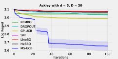
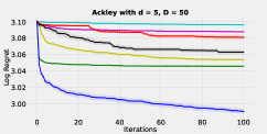
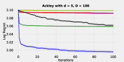
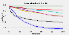
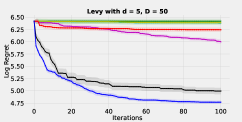
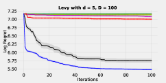
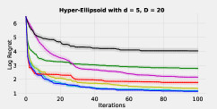
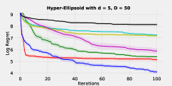
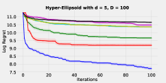
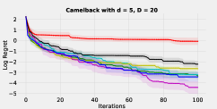
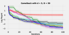
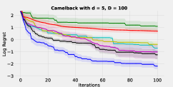
Figure 1: Comparison of baselines and the proposed MS-UCB method on four standard functions for 20, 50 and 100 input dimensions. For all cases, we set d=5๐‘‘5d=5 except LineBO and GP-UCB. The y๐‘ฆy-axis presents log distance to the true optimum (Smaller value is better).

To evaluate the performance of our MS-UCB, we have conducted a set of experiments involving optimization of four benchmark functions and two real applications. We compare our approach against six baselines: (1) Standard GP-UCB (?), (2) DropoutUCB (?), (3) LineBO (?) which restricts the search space to a one-dimensional subspace, (4) SRE (?) which uses sequential random embeddings several times sequentially, (5) REMBO (?), and (6) HeSBO (?) which use hashing-enhanced embedded subspaces. Among these baselines, the first three baselines do not make assumptions on the structure of the objective function, SRE assumes a tiny effect for some of the dimensions i.e. ฯตitalic-ฯต\epsilon-bounded while REMBO and HeSBO assume a low effective dimensional structure of the function.

For all experiments, we scale the search space of objective functions to convert into [โˆ’1,1]Dsuperscript11๐ท[-1,1]^{D}. We implemented our proposed MS-UCB, LineBO, DropoutUCB and SRE in Python 3 using GPy. For all other algorithms we used the authorsโ€™ reference implementations. For Gaussian process, we used Matern kernel and estimated the kernel hyper-parameters automatically from data. Each algorithm was randomly initialized with 20 points. To maximise the acquisition function, we used LBFGS-B algorithm with 10ร—D10๐ท10\times D random starts.

Optimization of Benchmark Functions

In this section, we test the algorithms on several optimization benchmark functions: Ackley, Levy, Hyper-Elippsoid and Camelback functions. For the first three functions we assume full dimensionality while for the two-dimensional Camelback function, we simulate a scenario so that the function has a low dimensional effective subspace. For this, we augment the Camelback function with auxiliary dimensions. The Ackley function is widely used for testing optimization algorithms. it is characterized by a nearly flat outer region while the Hyper-Elippsoid function is used to demonstrate that our algorithms can effectively work for functions with interacting variables. We evaluate the progress of each algorithm using the log distance to the true optimum, that is, log10โ€‹(fโ€‹(xโˆ—)โˆ’fโ€‹(xt))subscriptlog10๐‘“superscript๐‘ฅ๐‘“subscript๐‘ฅ๐‘ก\text{log}_{10}(f(x^{*})-f(x_{t})) where fโ€‹(xt)๐‘“subscript๐‘ฅ๐‘กf(x_{t}) is the function value sampled at iteration t๐‘กt. For each test function, we repeat the experiments 30 times. We plot the mean and a confidence bound of one standard deviation across all the runs.

On Scalability:

We perform experiments to empirically assess the scalability of our proposed MS-USB method and the baselines and report the results in Figure 1. We choose d=5๐‘‘5d=5 for all methods except LineBO for which d=1๐‘‘1d=1 is a requirement and the GP-UCB which works directly in original D๐ทD-dimensional space. We use N0=1,ฮฑ=0formulae-sequencesubscript๐‘01๐›ผ0N_{0}=1,\alpha=0 as parameters for our method. Recall that even with ฮฑ=0๐›ผ0\alpha=0, our method only has a sublinear cumulative regret growth. We study the cases with different input dimensions: (D=20,50,100)๐ท2050100(D=20,50,100). We can see that GP-UCB performs poorly in most cases on all test functions. The poor performance of GP-UCB is partly due to inaccurate solution of acquisition function optimisation in high dimensions. On the other hand, our method does better than all the baselines scaling well with the dimensions. Our method overcomes the difficulty by optimizing the acquisition function only on a set of d๐‘‘d-dimensional subspaces, and thus with a limited computation budget, the acquisition function optimisation is performed more accurately. Dropout and SRE that do not provide a vanishing regret scale poorly with high dimensions. LineBO performs poorly except for the Hyper-Ellipsoid function. For the Camelback function with just two effective dimensions, our method is still competitive to other methods that are designed to exploit such structure. Our method achieves a slightly better accuracy than SRE when D=50๐ท50D=50 and the best one when D=100๐ท100D=100. Thus our proposed MS-UCB outperforms baselines and scales well in high dimensions.

On the number of subspaces:

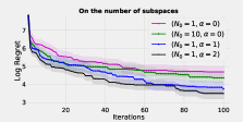
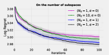
The number of subspaces per iteration is a control parameter in our method. It is set via N0subscript๐‘0N_{0} and in particular ฮฑ๐›ผ\alpha. In Theorem 3, we show that N0subscript๐‘0N_{0} does not affect much the regret. We study the effect of these parameters creating four MS-UCB variants: (N0=1,ฮฑ=0)formulae-sequencesubscript๐‘01๐›ผ0(N_{0}=1,\alpha=0), (N0=10,ฮฑ=0)formulae-sequencesubscript๐‘010๐›ผ0(N_{0}=10,\alpha=0), (N0=1,ฮฑ=1)formulae-sequencesubscript๐‘01๐›ผ1(N_{0}=1,\alpha=1) and finally (N0=1,ฮฑ=2)formulae-sequencesubscript๐‘01๐›ผ2(N_{0}=1,\alpha=2). We fix D=100๐ท100D=100 and d=5๐‘‘5d=5.

Refer to caption
(a) Hyper-Ellipsoid function
Refer to caption
(b) Ackley function
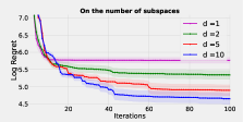
Figure 2: Log Regret vs iterations for varying number of subspaces (N0subscript๐‘0N_{0} and ฮฑ๐›ผ\alpha).

Figure 2 shows a comparison of these variants for Ackley function and Hyper-Ellipsoid function. It indicates if we increase N0subscript๐‘0N_{0} or ฮฑ๐›ผ\alpha (extending the search space), the regret decreases. For the case where ฮฑ=2๐›ผ2\alpha=2, we need to generate more subspaces at each iteration (at a quadratic rate: t2superscript๐‘ก2t^{2}). This demands more computational budget to maximise the acquisition function. It may be the reason why compared to case (N0=1,ฮฑ=0)formulae-sequencesubscript๐‘01๐›ผ0(N_{0}=1,\alpha=0), the regret of case (N0=1,ฮฑ=2)formulae-sequencesubscript๐‘01๐›ผ2(N_{0}=1,\alpha=2) improved only slightly.

On subspace dimension d๐‘‘d:

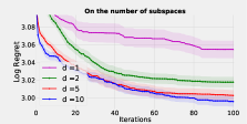
Dimension d๐‘‘d represents the dimension of the subspace. It directly affects the computational requirement of acquisition function maximization, and thus the BO optimization performance. As this computational requirement grows exponentially with increasing d๐‘‘d, it is often computationally hard to find the global maximum in more than 10 dimensions. Thus we only study the value of d๐‘‘d up to 10, i.e. we study cases: d=1,2,5,10๐‘‘12510d=1,2,5,10 for problems in D=100๐ท100D=100. We set N0=1,ฮฑ=0formulae-sequencesubscript๐‘01๐›ผ0N_{0}=1,\alpha=0 in our method. Figure 3 shows the performance of our method for different cases of d๐‘‘d for 100 dimensional Ackley function and Hyper-Ellipsoid function. It clearly indicates there is a faster convergence rate for a larger d๐‘‘d, though at a higher computational cost.
Refer to caption
(a) Hyper-Ellipsoid function
Refer to caption
(b) Ackley function
Figure 3: Log Regret vs iterations for varying dimension d๐‘‘d.

Learning Parameters of Machine Learning Models

Neural Network Parameter Search:

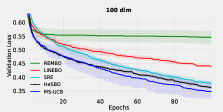
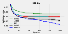
We evaluate our algorithm for learning the parameters of a neural network model as proposed by (?). Here we are given a neural network with one hidden layer having hโ„Žh nodes. The goal is to learn the weights between the hidden layer and the outputs in order to minimize the loss on the MNIST data set ((?)). We denote these weights by W2subscript๐‘Š2W_{2}. For all experiments, W2subscript๐‘Š2W_{2} is optimized by Bayesian optimization while the other weights and biases (we denote by W1subscript๐‘Š1W_{1}) are optimized by the Adam algorithm. We refer to (?) for more details. We try two cases: h=10โ„Ž10h=10 and h=50โ„Ž50h=50. Since the network has 10 outputs (for 10 digits of MNIST), the two cases lead to optimisation in dimensions 10ร—10=100101010010\times 10=100 and 50ร—10=500501050050\times 10=500 respectively. Figure 5 shows the validation loss for REMBO, LineBO, SRE, HeSBO and our proposed MS-UCB. As seen from the figure, MS-UCB clearly outperforms the baselines for both cases.
Refer to caption
(a)
Refer to caption
(b)
Figure 4: The neural network benchmark with target dimension d=10,N0=1,ฮฑ=1formulae-sequence๐‘‘10formulae-sequencesubscript๐‘01๐›ผ1d=10,N_{0}=1,\alpha=1 for two case where W2=10ร—10subscript๐‘Š21010W_{2}=10\times 10 and W2=50ร—10subscript๐‘Š25010W_{2}=50\times 10. For all experiments, W2subscript๐‘Š2W_{2} is optimized by Bayesian optimization while other weights and biases are optimized by Adam algorithm.

Learning Classification Model with Ramp Loss:

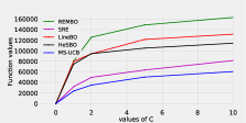
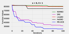
We also test our algorithm to optimize the parameters of a classification model with a nonconvex Ramp loss, following (?). The task is to find a vector w๐‘คw and a scalar b๐‘b to minimize fโ€‹(w,b)=12โ€‹โ€–wโ€–22+Cโ€‹โˆ‘l=1LRsโ€‹(ylโ€‹(wTโ€‹vl+b))๐‘“๐‘ค๐‘12superscriptsubscriptnorm๐‘ค22๐ถsuperscriptsubscript๐‘™1๐ฟsubscript๐‘…๐‘ subscript๐‘ฆ๐‘™subscript๐‘ค๐‘‡subscript๐‘ฃ๐‘™๐‘f(w,b)=\frac{1}{2}||w||_{2}^{2}+C\sum_{l=1}^{L}R_{s}(y_{l}(w_{T}v_{l}+b)), where vlsubscript๐‘ฃ๐‘™v_{l} are the training instances and ylโˆˆ{โˆ’1,+1}subscript๐‘ฆ๐‘™11y_{l}\in\{-1,+1\} are the corresponding labels. Rโ€‹sโ€‹(u)=H1โ€‹(u)โˆ’Hsโ€‹(u)๐‘…๐‘ ๐‘ขsubscript๐ป1๐‘ขsubscript๐ป๐‘ ๐‘ขRs(u)=H_{1}(u)-H_{s}(u) with s<1๐‘ 1s<1 where Hsโ€‹(u)=maxโ€‹(0,sโˆ’u)subscript๐ป๐‘ ๐‘ขmax0๐‘ ๐‘ขH_{s}(u)=\text{max}(0,s-u). We use the Gisette dataset from the UCI repository (?) with dimension D=5000๐ท5000D=5000. We study the effectiveness of all algorithms fixing the hyper-parameters to s=0๐‘ 0s=0 and Cโˆˆ{1,2,5,10}๐ถ12510C\in\{1,2,5,10\}. We set d=10๐‘‘10d=10 for REMBO, SRE, HeSBO and our method. For SRE, we set the number of sequential random embeddings m=5๐‘š5m=5 as suggested in (?). For our method, we consider the variant MS-UCB-1,1).
Refer to caption
(a)
Refer to caption
(b)
Figure 5: Left panel shows the progress of function values vs time for s=0๐‘ 0s=0 and C=1๐ถ1C=1. Right panel shows the comparison of achieved loss function values against the hyperparameter C๐ถC of the Ramp loss.

As shown in Figure 5, our method has consistently the best performance across different settings of C๐ถC, followed by SRE. REMBO, LineBO, HESBO perform poorly for this application. This shows the effectiveness of our method.

Conclusion

We propose a scalable Bayesian optimisation to optimise expensive blackbox functions in high dimensions. Unlike many previous existing methods, our algorithm does not make any additional assumption about the structure of the function (e.g. low effective dimension and additivity). In our method the acquisition function only requires maximisation on a discrete set of low dimensional subspaces embedded in the original high-dimensional search space and thus does not have high computational requirements for maximising acquisition functions. By varying the number of low dimensional subspaces, our algorithm has a flexibility to trade the optimisation convergence rate with the computational budget. This feature is important for many practical applications. We analyse our algorithm theoretically and show that irrespective of the number of subspaces, our algorithm always has a sublinear growth rate for cumulative regret. Further, we provide a regime for the number of subspaces where our algorithm has both tighter regret bound as well as lower computational requirement compared to the GP-UCB algorithm of (?). We perform experiments for many optimisation problems in high dimensions and show that the sample efficiency of our algorithm is better than the existing methods given the same computational budget for optimising acquisition function.

Acknowledgments

This research was partially funded by the Australian Government through the Australian Research Council (ARC). Prof Venkatesh is the recipient of an ARC Australian Laureate Fellowship (FL170100006).

References

  • [Chlebus 2009] Chlebus, E. 2009. An approximate formula for a partial sum of the divergent p-series. Appl. Math. Lett. 22:732โ€“737.
  • [Djolonga, Krause, and Cevher 2013] Djolonga, J.; Krause, A.; and Cevher, V. 2013. High-dimensional gaussian process bandits. In Proceedings of the 26th International Conference on Neural Information Processing Systems - Volume 1, NIPSโ€™13, 1025โ€“1033. USA: Curran Associates Inc.
  • [Eriksson et al. 2018] Eriksson, D.; Dong, K.; Lee, E.ย H.; Bindel, D.; and Wilson, A.ย G. 2018. Scaling gaussian process regression with derivatives. In Advances in Neural Information Processing Systems, 6868โ€“6878.
  • [Garnett, Osborne, and Hennig 2014] Garnett, R.; Osborne, M.ย A.; and Hennig, P. 2014. Active learning of linear embeddings for gaussian processes. In Proceedings of the Thirtieth Conference on Uncertainty in Artificial Intelligence, UAIโ€™14, 230โ€“239. Arlington, Virginia, United States: AUAI Press.
  • [Ghosal and Roy 2006] Ghosal, S., and Roy, A. 2006. Posterior consistency of gaussian process prior for nonparametric binary regression. Ann. Statist. 34(5):2413โ€“2429.
  • [Hoang et al. 2018] Hoang, T.ย N.; Hoang, Q.ย M.; Ouyang, R.; and Low, K.ย H. 2018. Decentralized high-dimensional bayesian optimization with factor graphs. In Proceedings of the Thirty-Second AAAI Conference on Artificial Intelligence (AAAI), 3231โ€“3238.
  • [Kandasamy 2015] Kandasamy. 2015. High dimensional bayesian optimisation and bandits via additive models. In Proceedings of the 32Nd International Conference on International Conference on Machine Learning - Volume 37, ICMLโ€™15, 295โ€“304. JMLR.org.
  • [Kirschner et al. 2019] Kirschner, J.; Mutny, M.; Hiller, N.; Ischebeck, R.; and Krause, A. 2019. Adaptive and safe Bayesian optimization in high dimensions via one-dimensional subspaces. In Chaudhuri, K., and Salakhutdinov, R., eds., Proceedings of the 36th International Conference on Machine Learning, volumeย 97 of Proceedings of Machine Learning Research, 3429โ€“3438. Long Beach, California, USA: PMLR.
  • [LeCun and Cortes 2010] LeCun, Y., and Cortes, C. 2010. MNIST handwritten digit database.
  • [Li et al. 2017] Li, C.; Gupta, S.; Rana, S.; Nguyen, V.; Venkatesh, S.; and Shilton, A. 2017. High dimensional bayesian optimization using dropout. In Proceedings of the 26th International Joint Conference on Artificial Intelligence, IJCAIโ€™17, 2096โ€“2102. AAAI Press.
  • [Li 2016] Li, C.-L. 2016. High dimensional bayesian optimization via restricted projection pursuit models. In Gretton, A., and Robert, C.ย C., eds., Proceedings of the 19th International Conference on Artificial Intelligence and Statistics, volumeย 51 of Proceedings of Machine Learning Research, 884โ€“892. Cadiz, Spain: PMLR.
  • [Mockus 1974] Mockus, J. 1974. On bayesian methods for seeking the extremum. In Proceedings of the IFIP Technical Conference, 400โ€“404. London, UK, UK: Springer-Verlag.
  • [Mutnรฝ and Krause 2018] Mutnรฝ, M., and Krause, A. 2018. Efficient high dimensional bayesian optimization with additivity and quadrature fourier features. In Proceedings of the 32Nd International Conference on Neural Information Processing Systems, NIPSโ€™18, 9019โ€“9030. USA: Curran Associates Inc.
  • [Nayebi, Munteanu, and Poloczek 2019] Nayebi, A.; Munteanu, A.; and Poloczek, M. 2019. A framework for Bayesian optimization in embedded subspaces. In Chaudhuri, K., and Salakhutdinov, R., eds., Proceedings of the 36th International Conference on Machine Learning, volumeย 97 of Proceedings of Machine Learning Research, 4752โ€“4761. Long Beach, California, USA: PMLR.
  • [Newman and Merz 1998] Newman, C. B.ย D., and Merz, C. 1998. UCI repository of machine learning databases.
  • [Oh, Gavves, and Welling 2018] Oh, C.; Gavves, E.; and Welling, M. 2018. BOCK : Bayesian optimization with cylindrical kernels. In ICML, volumeย 80 of Proceedings of Machine Learning Research, 3865โ€“3874. PMLR.
  • [Qian, Hu, and Yu 2016] Qian, H.; Hu, Y.-Q.; and Yu, Y. 2016. Derivative-free optimization of high-dimensional non-convex functions by sequential random embeddings. In Proceedings of the Twenty-Fifth International Joint Conference on Artificial Intelligence, IJCAIโ€™16, 1946โ€“1952. AAAI Press.
  • [Rana et al. 2017] Rana, S.; Li, C.; Gupta, S.; Nguyen, V.; and Venkatesh, S. 2017. High dimensional bayesian optimization with elastic gaussian process. In Proceedings of the 34th International Conference on Machine Learning - Volume 70, ICMLโ€™17, 2883โ€“2891. JMLR.org.
  • [Rasmussen and Williams 2005] Rasmussen, C.ย E., and Williams, C. K.ย I. 2005. Gaussian Processes for Machine Learning (Adaptive Computation and Machine Learning). The MIT Press.
  • [Rolland et al. 2018] Rolland, P.; Scarlett, J.; Bogunovic, I.; and Cevher, V. 2018. High-dimensional bayesian optimization via additive models with overlapping groups. In Storkey, A., and Perez-Cruz, F., eds., Proceedings of the Twenty-First International Conference on Artificial Intelligence and Statistics, volumeย 84 of Proceedings of Machine Learning Research, 298โ€“307. Playa Blanca, Lanzarote, Canary Islands: PMLR.
  • [Srinivas et al. 2012] Srinivas, N.; Krause, A.; Kakade, S.ย M.; and Seeger, M.ย W. 2012. Information-theoretic regret bounds for gaussian process optimization in the bandit setting. IEEE Trans. Inf. Theor. 58(5):3250โ€“3265.
  • [Wang et al. 2013] Wang, Z.; Zoghi, M.; Hutter, F.; Matheson, D.; and Deย Freitas, N. 2013. Bayesian optimization in high dimensions via random embeddings. In Proceedings of the Twenty-Third International Joint Conference on Artificial Intelligence, IJCAI โ€™13, 1778โ€“1784. AAAI Press.
  • [Wang 2005] Wang, X. 2005. Volumes of generalized unit balls. Mathematics Magazine 78(5):390 โ€“ 395.
  • [Zhang, Li, and Su 2019] Zhang, M.; Li, H.; and Su, S.ย W. 2019. High dimensional bayesian optimization via supervised dimension reduction. CoRR abs/1907.08953.

Supplementary Material

Proof for Lemma 2

Given ฮฒt0superscriptsubscript๐›ฝ๐‘ก0\beta_{t}^{0}, we have โ„™โ€‹[|fโ€‹(xt)โˆ’ฮผtโˆ’1โ€‹(xt)|>ฮฒt0]โ‰คeฮฒt0/2โ„™delimited-[]๐‘“subscript๐‘ฅ๐‘กsubscript๐œ‡๐‘ก1subscript๐‘ฅ๐‘กsuperscriptsubscript๐›ฝ๐‘ก0superscript๐‘’superscriptsubscript๐›ฝ๐‘ก02\mathbb{P}[|f(x_{t})-\mu_{t-1}(x_{t})|>\sqrt{\beta_{t}^{0}}]\leq e^{\beta_{t}^{0}/2}. Since eฮฒt0/2=6โ€‹ฮดฯ€2โ€‹t2superscript๐‘’superscriptsubscript๐›ฝ๐‘ก026๐›ฟsuperscript๐œ‹2superscript๐‘ก2e^{\beta_{t}^{0}/2}=\frac{6\delta}{\pi^{2}t^{2}}. Using the union bound for tโˆˆโ„•๐‘กโ„•t\ \in\mathbb{N}, we have โ„™โ€‹[|fโ€‹(xt)โˆ’ฮผtโˆ’1โ€‹(xt)|โ‰คฮฒt0]โ‰ฅ1โˆ’ฯ€2โ€‹ฮด6>1โˆ’ฮดโ„™delimited-[]๐‘“subscript๐‘ฅ๐‘กsubscript๐œ‡๐‘ก1subscript๐‘ฅ๐‘กsuperscriptsubscript๐›ฝ๐‘ก01superscript๐œ‹2๐›ฟ61๐›ฟ\mathbb{P}[|f(x_{t})-\mu_{t-1}(x_{t})|\leq\sqrt{\beta_{t}^{0}}]\geq 1-\frac{\pi^{2}\delta}{6}>1-\delta.

Proof for Lemma 3

We use the idea of proof of Lemma 5.7 in (?) with several modifications to adapt our method with low-dimensional subspaces. We consider the distance of any two points on subspace ๐’ฎโ€‹(A,ztโˆ—)๐’ฎ๐ดsubscriptsuperscript๐‘ง๐‘ก\mathcal{S}(A,z^{*}_{t}): โ€–(Aโ€‹y+Bโ€‹ztโˆ—)โˆ’(Aโ€‹yโ€ฒ+Bโ€‹ztโˆ—)โ€–1subscriptnorm๐ด๐‘ฆ๐ตsubscriptsuperscript๐‘ง๐‘ก๐ดsuperscript๐‘ฆโ€ฒ๐ตsubscriptsuperscript๐‘ง๐‘ก1||(Ay+Bz^{*}_{t})-(Ay^{\prime}+Bz^{*}_{t})||_{1}, where y,yโ€ฒโˆˆ๐’ด๐‘ฆsuperscript๐‘ฆโ€ฒ๐’ดy,y^{\prime}\in\mathcal{Y}. We have matrix A=[๐ŸŽ๐ˆ]๐ดmatrix0๐ˆA=\begin{bmatrix}\mathbf{0}\\ \mathbf{I}\end{bmatrix}, thus ||(Ay+Bztโˆ—)โˆ’(Ayโ€ฒ+Bztโˆ—)||1=โˆ‘i=1D|[A(yโˆ’yโ€ฒ)]i|=โˆ‘i=1Dโˆ’d|[๐ŸŽ(Dโˆ’d)ร—d(yโˆ’yโ€ฒ)]i)|+โˆ‘i=Dโˆ’d+1D|[๐ˆdร—d(yโˆ’yโ€ฒ)]i|=โˆ‘i=Dโˆ’d+1D|[(yโˆ’yโ€ฒ)]i|||(Ay+Bz^{*}_{t})-(Ay^{\prime}+Bz^{*}_{t})||_{1}=\sum_{i=1}^{D}|[A(y-y^{\prime})]_{i}|=\sum_{i=1}^{D-d}|[\mathbf{0}^{(D-d)\times d}(y-y^{\prime})]_{i})|+\sum_{i=D-d+1}^{D}|[\mathbf{I}^{d\times d}(y-y^{\prime})]_{i}|=\sum_{i=D-d+1}^{D}|[(y-y^{\prime})]_{i}|, where we denote [y]isubscriptdelimited-[]๐‘ฆ๐‘–[y]_{i} is the i๐‘–ith coordinate of y๐‘ฆy. However, since for every 1โ‰คiโ‰คDโˆ’d,1โ‰คjโ‰คdformulae-sequence1๐‘–๐ท๐‘‘1๐‘—๐‘‘1\leq i\leq D-d,1\leq j\leq d and |[yโˆ’yโ€ฒ]i|โ‰ค2subscriptdelimited-[]๐‘ฆsuperscript๐‘ฆโ€ฒ๐‘–2|[y-y^{\prime}]_{i}|\leq 2 for every y,yโ€ฒโˆˆ[โˆ’1,1]d๐‘ฆsuperscript๐‘ฆโ€ฒsuperscript11๐‘‘y,y^{\prime}\in[-1,1]^{d}, โˆ‘i=Dโˆ’d+1D|[(yโˆ’yโ€ฒ)]i|โ‰ค2โ€‹dsuperscriptsubscript๐‘–๐ท๐‘‘1๐ทsubscriptdelimited-[]๐‘ฆsuperscript๐‘ฆโ€ฒ๐‘–2๐‘‘\sum_{i=D-d+1}^{D}|[(y-y^{\prime})]_{i}|\leq 2d. Thus, โ€–(Aโ€‹y+Bโ€‹ztโˆ—)โˆ’(Aโ€‹yโ€ฒ+Bโ€‹ztโˆ—)โ€–1โ‰ค2โ€‹dsubscriptnorm๐ด๐‘ฆ๐ตsubscriptsuperscript๐‘ง๐‘ก๐ดsuperscript๐‘ฆโ€ฒ๐ตsubscriptsuperscript๐‘ง๐‘ก12๐‘‘||(Ay+Bz^{*}_{t})-(Ay^{\prime}+Bz^{*}_{t})||_{1}\leq 2d.

On the other hand, by Assumption 1 and the union bound, for โˆ€x,xโ€ฒโˆˆ๐’ฎโ€‹(A,ztโˆ—)for-all๐‘ฅsuperscript๐‘ฅโ€ฒ๐’ฎ๐ดsubscriptsuperscript๐‘ง๐‘ก\forall x,x^{\prime}\in\mathcal{S}(A,z^{*}_{t}) and thus โˆˆ๐’ณabsent๐’ณ\in\mathcal{X}, we have

|fโ€‹(x)โˆ’fโ€‹(xโ€ฒ)|โ‰คLโ€‹โ€–xโˆ’xโ€ฒโ€–1๐‘“๐‘ฅ๐‘“superscript๐‘ฅโ€ฒ๐ฟsubscriptnorm๐‘ฅsuperscript๐‘ฅโ€ฒ1|f(x)-f(x^{\prime})|\leq L||x-x^{\prime}||_{1}

with probability greater than 1โˆ’Dโ€‹aโ€‹eโˆ’L2/b21๐ท๐‘Žsuperscript๐‘’superscript๐ฟ2superscript๐‘21-Dae^{-L^{2}/b^{2}}. Thus, by choosing Dโ€‹aโ€‹eโˆ’L2/b2=ฮด/2๐ท๐‘Žsuperscript๐‘’superscript๐ฟ2superscript๐‘2๐›ฟ2Dae^{-L^{2}/b^{2}}=\delta/2, we have

|fโ€‹(x)โˆ’fโ€‹(xโ€ฒ)|โ‰คbโ€‹lโ€‹oโ€‹gโ€‹(2โ€‹Dโ€‹aฮด)โ€‹โ€–xโˆ’xโ€ฒโ€–1๐‘“๐‘ฅ๐‘“superscript๐‘ฅโ€ฒ๐‘๐‘™๐‘œ๐‘”2๐ท๐‘Ž๐›ฟsubscriptnorm๐‘ฅsuperscript๐‘ฅโ€ฒ1\displaystyle|f(x)-f(x^{\prime})|\leq b\sqrt{log(\frac{2Da}{\delta})}||x-x^{\prime}||_{1} (14)

with probability greater than 1โˆ’ฮด/21๐›ฟ21-\delta/2.

Now, we move to subspace ๐’ฎโ€‹(A,ztโˆ—)๐’ฎ๐ดsubscriptsuperscript๐‘ง๐‘ก\mathcal{S}(A,z^{*}_{t}). On ๐’ฎโ€‹(A,ztโˆ—)๐’ฎ๐ดsubscriptsuperscript๐‘ง๐‘ก\mathcal{S}(A,z^{*}_{t}), we construct a discretization Ftsubscript๐น๐‘กF_{t} of size (ฯ„t)dsuperscriptsubscript๐œ๐‘ก๐‘‘(\tau_{t})^{d} dense enough such that for any xโˆˆFt๐‘ฅsubscript๐น๐‘กx\in F_{t}

||xโˆ’[x]t]||1โ‰ค2โ€‹dฯ„t||x-[x]_{t}]||_{1}\leq\frac{2d}{\tau_{t}}

where [x]tsubscriptdelimited-[]๐‘ฅ๐‘ก[x]_{t} denotes the closest point in Ftsubscript๐น๐‘กF_{t} to x๐‘ฅx. We can perform this because the distance between any two point in ๐’ฎโ€‹(A,ztโˆ—)๐’ฎ๐ดsubscriptsuperscript๐‘ง๐‘ก\mathcal{S}(A,z^{*}_{t}) is bounded by 2โ€‹d2๐‘‘2d in the above proof.

By this manner, with probability greater than 1โˆ’ฮด/21๐›ฟ21-\delta/2, we have

|fโ€‹(x)โˆ’fโ€‹([x]t)|๐‘“๐‘ฅ๐‘“subscriptdelimited-[]๐‘ฅ๐‘ก\displaystyle|f(x)-f([x]_{t})| โ‰ค\displaystyle\leq bโ€‹lโ€‹oโ€‹gโ€‹(2โ€‹Dโ€‹aฮด)โ€‹โ€–xโˆ’[x]tโ€–1ฯ„t๐‘๐‘™๐‘œ๐‘”2๐ท๐‘Ž๐›ฟsubscriptnorm๐‘ฅsubscriptdelimited-[]๐‘ฅ๐‘ก1subscript๐œ๐‘ก\displaystyle\frac{b\sqrt{log(\frac{2Da}{\delta})}||x-[x]_{t}||_{1}}{\tau_{t}}
โ‰ค\displaystyle\leq bโ€‹lโ€‹oโ€‹gโ€‹(2โ€‹Dโ€‹aฮด)โ€‹2โ€‹dฯ„t๐‘๐‘™๐‘œ๐‘”2๐ท๐‘Ž๐›ฟ2๐‘‘subscript๐œ๐‘ก\displaystyle b\sqrt{log(\frac{2Da}{\delta})}\frac{2d}{\tau_{t}}
<\displaystyle< 2โ€‹bโ€‹dโ€‹lโ€‹oโ€‹gโ€‹(2โ€‹Dโ€‹aฮด)ฯ„t2๐‘๐‘‘๐‘™๐‘œ๐‘”2๐ท๐‘Ž๐›ฟsubscript๐œ๐‘ก\displaystyle\frac{2bd\sqrt{log(\frac{2Da}{\delta})}}{\tau_{t}}

Let ฯ„t=2โ€‹bโ€‹dโ€‹lโ€‹oโ€‹gโ€‹(2โ€‹Dโ€‹aฮด)โ€‹t2subscript๐œ๐‘ก2๐‘๐‘‘๐‘™๐‘œ๐‘”2๐ท๐‘Ž๐›ฟsuperscript๐‘ก2\tau_{t}=2bd\sqrt{log(\frac{2Da}{\delta})}t^{2}. Thus, |Ft|=(2โ€‹bโ€‹dโ€‹lโ€‹oโ€‹gโ€‹(2โ€‹Dโ€‹aฮด)โ€‹t2)dsubscript๐น๐‘กsuperscript2๐‘๐‘‘๐‘™๐‘œ๐‘”2๐ท๐‘Ž๐›ฟsuperscript๐‘ก2๐‘‘|F_{t}|=(2bd\sqrt{log(\frac{2Da}{\delta})}t^{2})^{d}. We obtain

|fโ€‹(x)โˆ’fโ€‹([x]t)|โ‰ค1t2๐‘“๐‘ฅ๐‘“subscriptdelimited-[]๐‘ฅ๐‘ก1superscript๐‘ก2\displaystyle|f(x)-f([x]_{t})|\leq\frac{1}{t^{2}} (15)

with probability 1โˆ’ฮด/21๐›ฟ21-\delta/2 for any xโˆˆFt๐‘ฅsubscript๐น๐‘กx\in F_{t}.

Similar to Lemma 5.6 of (?), if we set ฮฒt1=2โ€‹lโ€‹oโ€‹gโ€‹(|Ft|โ€‹ฯ€2โ€‹t23โ€‹ฮด)=2โ€‹lโ€‹oโ€‹gโ€‹(ฯ€2โ€‹t23โ€‹ฮด)+2โ€‹dโ€‹lโ€‹oโ€‹gโ€‹(2โ€‹bโ€‹dโ€‹lโ€‹oโ€‹gโ€‹(2โ€‹Dโ€‹aฮด)โ€‹t2)superscriptsubscript๐›ฝ๐‘ก12๐‘™๐‘œ๐‘”subscript๐น๐‘กsuperscript๐œ‹2superscript๐‘ก23๐›ฟ2๐‘™๐‘œ๐‘”superscript๐œ‹2superscript๐‘ก23๐›ฟ2๐‘‘๐‘™๐‘œ๐‘”2๐‘๐‘‘๐‘™๐‘œ๐‘”2๐ท๐‘Ž๐›ฟsuperscript๐‘ก2\beta_{t}^{1}=2log(|F_{t}|\frac{\pi^{2}t^{2}}{3\delta})=2log(\frac{\pi^{2}t^{2}}{3\delta})+2dlog(2bd\sqrt{log(\frac{2Da}{\delta})}t^{2}), we have with probability 1โˆ’ฮด/21๐›ฟ21-\delta/2, we have

fโ€‹(x)โ‰คฮผtโˆ’1โ€‹(x)+ฮฒt1โ€‹ฯƒtโˆ’1โ€‹(x)๐‘“๐‘ฅsubscript๐œ‡๐‘ก1๐‘ฅsuperscriptsubscript๐›ฝ๐‘ก1subscript๐œŽ๐‘ก1๐‘ฅ\displaystyle f(x)\leq\mu_{t-1}(x)+\sqrt{\beta_{t}^{1}}\sigma_{t-1}(x) (16)

for any xโˆˆFt๐‘ฅsubscript๐น๐‘กx\in F_{t} and any tโ‰ฅ1๐‘ก1t\geq 1. Thus, combining Eq(15) and Eq(16), if we let xโ€ฒ=[Aโ€‹yโˆ—+Bโ€‹ztโˆ—]tsuperscript๐‘ฅโ€ฒsubscriptdelimited-[]๐ดsuperscript๐‘ฆ๐ตsubscriptsuperscript๐‘ง๐‘ก๐‘กx^{\prime}=[Ay^{*}+Bz^{*}_{t}]_{t} which is the closest point in Ftsubscript๐น๐‘กF_{t} to Aโ€‹yโˆ—+Bโ€‹ztโˆ—๐ดsuperscript๐‘ฆ๐ตsubscriptsuperscript๐‘ง๐‘กAy^{*}+Bz^{*}_{t}, we have

f๐’ฎt0mโ€‹aโ€‹xsubscriptsuperscript๐‘“๐‘š๐‘Ž๐‘ฅsuperscriptsubscript๐’ฎ๐‘ก0\displaystyle f^{max}_{\mathcal{S}_{t}^{0}} =\displaystyle= fโ€‹(Aโ€‹yโˆ—+Bโ€‹ztโˆ—)๐‘“๐ดsuperscript๐‘ฆ๐ตsubscriptsuperscript๐‘ง๐‘ก\displaystyle f(Ay^{*}+Bz^{*}_{t})
โ‰ค\displaystyle\leq fโ€‹([Aโ€‹yโˆ—+Bโ€‹ztโˆ—]t)+1t2๐‘“subscriptdelimited-[]๐ดsuperscript๐‘ฆ๐ตsubscriptsuperscript๐‘ง๐‘ก๐‘ก1superscript๐‘ก2\displaystyle f([Ay^{*}+Bz^{*}_{t}]_{t})+\frac{1}{t^{2}}
โ‰ค\displaystyle\leq ฮผtโˆ’1โ€‹(xโ€ฒ)+ฮฒt1โ€‹ฯƒtโˆ’1โ€‹(xโ€ฒ)+1t2subscript๐œ‡๐‘ก1superscript๐‘ฅโ€ฒsuperscriptsubscript๐›ฝ๐‘ก1subscript๐œŽ๐‘ก1superscript๐‘ฅโ€ฒ1superscript๐‘ก2\displaystyle\mu_{t-1}(x^{\prime})+\sqrt{\beta_{t}^{1}}\sigma_{t-1}(x^{\prime})+\frac{1}{t^{2}}

with probability 1โˆ’ฮด1๐›ฟ1-\delta. Note that since xโ€ฒโˆˆFtsuperscript๐‘ฅโ€ฒsubscript๐น๐‘กx^{\prime}\in F_{t}, xโ€ฒโˆˆ๐’ฎโ€‹(A,ztโˆ—)superscript๐‘ฅโ€ฒ๐’ฎ๐ดsubscriptsuperscript๐‘ง๐‘กx^{\prime}\in\mathcal{S}(A,z^{*}_{t}).

Proof for Lemma 4

Given any xโˆˆ๐’ฎt0๐‘ฅsuperscriptsubscript๐’ฎ๐‘ก0x\in\mathcal{S}_{t}^{0}. Without loss of generality, we assume that x=Aโ€‹yโˆ—+Bโ€‹z๐‘ฅ๐ดsuperscript๐‘ฆ๐ต๐‘งx=Ay^{*}+Bz, where zโˆˆZt๐‘งsubscript๐‘๐‘กz\in Z_{t}. By Assumption 1 and the union bound, we have that for โˆ€๐ฑfor-all๐ฑ\forall\mathbf{x},

|f(xโˆ—)โˆ’f(x)|โ‰คL||xโˆ—โˆ’x)||1|f(x^{*})-f(x)|\leq L||x^{*}-x)||_{1}

with probability greater than 1โˆ’Dโ€‹aโ€‹eโˆ’L2/b21๐ท๐‘Žsuperscript๐‘’superscript๐ฟ2superscript๐‘21-Dae^{-L^{2}/b^{2}}. Since xโˆ—=Aโ€‹yโˆ—+Bโ€‹zโˆ—superscript๐‘ฅ๐ดsuperscript๐‘ฆ๐ตsuperscript๐‘งx^{*}=Ay^{*}+Bz^{*} and x=Aโ€‹yโˆ—+Bโ€‹z๐‘ฅ๐ดsuperscript๐‘ฆ๐ต๐‘งx=Ay^{*}+Bz, โ€–xโˆ—โˆ’xโ€–1=โ€–Aโ€‹yโˆ—+Bโ€‹zโˆ—โˆ’(Aโ€‹yโˆ—+Bโ€‹z)โ€–1=โ€–zโˆ’zโˆ—โ€–1subscriptnormsuperscript๐‘ฅ๐‘ฅ1subscriptnorm๐ดsuperscript๐‘ฆ๐ตsuperscript๐‘ง๐ดsuperscript๐‘ฆ๐ต๐‘ง1subscriptnorm๐‘งsuperscript๐‘ง1||x^{*}-x||_{1}=||Ay^{*}+Bz^{*}-(Ay^{*}+Bz)||_{1}=||z-z^{*}||_{1}. Thus,

|fโ€‹(xโˆ—)โˆ’fโ€‹(x)|โ‰คLโ€‹โ€–zโˆ—โˆ’zโ€–1๐‘“superscript๐‘ฅ๐‘“๐‘ฅ๐ฟsubscriptnormsuperscript๐‘ง๐‘ง1|f(x^{*})-f(x)|\leq L||z^{*}-z||_{1}

with probability greater than 1โˆ’Dโ€‹aโ€‹eโˆ’L2/b21๐ท๐‘Žsuperscript๐‘’superscript๐ฟ2superscript๐‘21-Dae^{-L^{2}/b^{2}}. Set Dโ€‹aโ€‹eโˆ’L2/b2=ฮด/2๐ท๐‘Žsuperscript๐‘’superscript๐ฟ2superscript๐‘2๐›ฟ2Dae^{-L^{2}/b^{2}}=\delta/2. Thus,

|fโ€‹(xโˆ—)โˆ’fโ€‹(x)|โ‰คbโ€‹lโ€‹oโ€‹gโ€‹(2โ€‹Dโ€‹aฮด)โ€‹โ€–zโˆ—โˆ’zโ€–1๐‘“superscript๐‘ฅ๐‘“๐‘ฅ๐‘๐‘™๐‘œ๐‘”2๐ท๐‘Ž๐›ฟsubscriptnormsuperscript๐‘ง๐‘ง1\displaystyle|f(x^{*})-f(x)|\leq b\sqrt{log(\frac{2Da}{\delta})}||z^{*}-z||_{1} (17)

with probability greater than 1โˆ’ฮด/21๐›ฟ21-\delta/2

We denote the volume of space ๐’ต๐’ต\mathcal{Z} be Vโ€‹oโ€‹lโ€‹(๐’ต)๐‘‰๐‘œ๐‘™๐’ตVol(\mathcal{Z}). Since zโˆˆ[โˆ’1,1]Dโˆ’d๐‘งsuperscript11๐ท๐‘‘z\in[-1,1]^{D-d}, Vโ€‹oโ€‹lโ€‹(๐’ต)=2Dโˆ’d๐‘‰๐‘œ๐‘™๐’ตsuperscript2๐ท๐‘‘Vol(\mathcal{Z})=2^{D-d}. For ฮธ>0๐œƒ0\theta>0, let V1={zโˆˆ๐’ต=[โˆ’1,1]Dโˆ’d|โ€–zโˆ’zโˆ—โ€–1โ‰คฮธ}subscript๐‘‰1conditional-set๐‘ง๐’ตsuperscript11๐ท๐‘‘subscriptnorm๐‘งsuperscript๐‘ง1๐œƒV_{1}=\{z\in\mathcal{Z}=[-1,1]^{D-d}|||z-z^{*}||_{1}\leq\theta\}. In the case where V1subscript๐‘‰1V_{1} is within ๐’ต๐’ต\mathcal{Z}, the volume Vโ€‹oโ€‹lโ€‹(V1)๐‘‰๐‘œ๐‘™subscript๐‘‰1Vol(V_{1}) is the volume of a (Dโˆ’d)๐ท๐‘‘(D-d)-dimensional ball of radius ฮธ๐œƒ\theta with center zโˆ—superscript๐‘งz^{*} and thus, Vโ€‹oโ€‹lโ€‹(V1)=(4โ€‹ฮธ)Dโˆ’dฮ“โ€‹(Dโˆ’d+1)๐‘‰๐‘œ๐‘™subscript๐‘‰1superscript4๐œƒ๐ท๐‘‘ฮ“๐ท๐‘‘1Vol(V_{1})=\frac{(4\theta)^{D-d}}{\Gamma(D-d+1)} where ฮ“ฮ“\Gamma is Leonhard Eulerโ€™s Gamma function. The function ฮ“โ€‹(k)=(kโˆ’1)!ฮ“๐‘˜๐‘˜1\Gamma(k)=(k-1)! for any positive integer k๐‘˜k. Here, we used the formula in (?) for the volume of the (Dโˆ’d)๐ท๐‘‘(D-d)-dimensional ball in L1superscript๐ฟ1L^{1} norms. In the worst case where zโˆ—superscript๐‘งz^{*} is at the boundary of ๐’ต๐’ต\mathcal{Z}, more precisely either [zโˆ—]i=1subscriptdelimited-[]superscript๐‘ง๐‘–1[z^{*}]_{i}=1 or [zโˆ—]i=โˆ’1subscriptdelimited-[]superscript๐‘ง๐‘–1[z^{*}]_{i}=-1 for any 1โ‰คiโ‰คDโˆ’d1๐‘–๐ท๐‘‘1\leq i\leq D-d, Vโ€‹oโ€‹lโ€‹(V1)๐‘‰๐‘œ๐‘™subscript๐‘‰1Vol(V_{1}) is at least (2โ€‹ฮธ)Dโˆ’dฮ“โ€‹(Dโˆ’d+1)superscript2๐œƒ๐ท๐‘‘ฮ“๐ท๐‘‘1\frac{(2\theta)^{D-d}}{\Gamma(D-d+1)}. This is because the volume halved by each dimension: ๐’ซโ€‹[|[z]iโˆ’[zโˆ—]i|โ‰คฮธ]=ฮธ2๐’ซdelimited-[]subscriptdelimited-[]๐‘ง๐‘–subscriptdelimited-[]superscript๐‘ง๐‘–๐œƒ๐œƒ2\mathcal{P}[|[z]_{i}-[z^{*}]_{i}|\leq\theta]=\frac{\theta}{2} when [zโˆ—]i=1subscriptdelimited-[]superscript๐‘ง๐‘–1[z^{*}]_{i}=1 or โˆ’11-1. Thus, in every case, we have Vโ€‹oโ€‹lโ€‹(V1)โ‰ฅ(2โ€‹ฮธ)Dโˆ’dฮ“โ€‹(Dโˆ’d+1)๐‘‰๐‘œ๐‘™subscript๐‘‰1superscript2๐œƒ๐ท๐‘‘ฮ“๐ท๐‘‘1Vol(V_{1})\geq\frac{(2\theta)^{D-d}}{\Gamma(D-d+1)}.

Thus, โ„™โ€‹[โ€–zโˆ’zโˆ—โ€–1โ‰คฮธ]=Vโ€‹oโ€‹lโ€‹(V1)Vโ€‹oโ€‹lโ€‹(๐’ต)โ‰ฅ(2โ€‹ฮธ)Dโˆ’dฮ“โ€‹(Dโˆ’d+1)2Dโˆ’d=ฮธDโˆ’dฮ“โ€‹(Dโˆ’d+1)โ„™delimited-[]subscriptnorm๐‘งsuperscript๐‘ง1๐œƒ๐‘‰๐‘œ๐‘™subscript๐‘‰1๐‘‰๐‘œ๐‘™๐’ตsuperscript2๐œƒ๐ท๐‘‘ฮ“๐ท๐‘‘1superscript2๐ท๐‘‘superscript๐œƒ๐ท๐‘‘ฮ“๐ท๐‘‘1\mathbb{P}[||z-z^{*}||_{1}\leq\theta]=\frac{Vol(V_{1})}{Vol(\mathcal{Z})}\geq\frac{\frac{(2\theta)^{D-d}}{\Gamma(D-d+1)}}{2^{D-d}}=\frac{\theta^{D-d}}{\Gamma(D-d+1)}. However, โ„™โ€‹[โ€–zโˆ’zโˆ—โ€–1>ฮธ]=1โˆ’โ„™โ€‹[โ€–zโˆ’zโˆ—โ€–1โ‰คฮธ]โ„™delimited-[]subscriptnorm๐‘งsuperscript๐‘ง1๐œƒ1โ„™delimited-[]subscriptnorm๐‘งsuperscript๐‘ง1๐œƒ\mathbb{P}[||z-z^{*}||_{1}>\theta]=1-\mathbb{P}[||z-z^{*}||_{1}\leq\theta]. Thus, โ„™โ€‹[โ€–zโˆ’zโˆ—โ€–1>ฮธ]โ‰ค1โˆ’ฮธDโˆ’dฮ“โ€‹(Dโˆ’d+1)โ‰คeโˆ’ฮธDโˆ’dฮ“โ€‹(Dโˆ’d+1)โ„™delimited-[]subscriptnorm๐‘งsuperscript๐‘ง1๐œƒ1superscript๐œƒ๐ท๐‘‘ฮ“๐ท๐‘‘1superscript๐‘’superscript๐œƒ๐ท๐‘‘ฮ“๐ท๐‘‘1\mathbb{P}[||z-z^{*}||_{1}>\theta]\leq 1-\frac{\theta^{D-d}}{\Gamma(D-d+1)}\leq e^{-\frac{\theta^{D-d}}{\Gamma(D-d+1)}}, where we use the inequality 1โˆ’xโ‰คeโˆ’x1๐‘ฅsuperscript๐‘’๐‘ฅ1-x\leq e^{-x} for the last step.

Thus,

โˆzโˆˆ๐’ตtโ„™โ€‹[โ€–zโˆ’zโˆ—โ€–1>ฮธ]subscriptproduct๐‘งsubscript๐’ต๐‘กโ„™delimited-[]subscriptnorm๐‘งsuperscript๐‘ง1๐œƒ\displaystyle\prod_{z\in\mathcal{Z}_{t}}\mathbb{P}[||z-z^{*}||_{1}>\theta] โ‰ค\displaystyle\leq โˆzโˆˆ๐’ตteโˆ’ฮธDโˆ’dฮ“โ€‹(Dโˆ’d+1)subscriptproduct๐‘งsubscript๐’ต๐‘กsuperscript๐‘’superscript๐œƒ๐ท๐‘‘ฮ“๐ท๐‘‘1\displaystyle\prod_{z\in\mathcal{Z}_{t}}e^{-\frac{\theta^{D-d}}{\Gamma(D-d+1)}}
=\displaystyle= eโˆ’|Zt|โ€‹ฮธDโˆ’dฮ“โ€‹(Dโˆ’d+1)superscript๐‘’subscript๐‘๐‘กsuperscript๐œƒ๐ท๐‘‘ฮ“๐ท๐‘‘1\displaystyle e^{-|Z_{t}|\frac{\theta^{D-d}}{\Gamma(D-d+1)}}

On the other hand, โ„™โ€‹[โ€–ztโˆ—โˆ’zโˆ—โ€–1โ‰คฮธ]=1โˆ’โ„™โ€‹[โ€–ztโˆ—โˆ’zโˆ—โ€–1>ฮธ]=1โˆ’โ„™ztiโˆˆ๐’ตt,1โ‰คiโ‰ค|Zt|โ€‹[โ€–zt1โˆ’zโˆ—โ€–1>ฮธโˆงโ€ฆโˆงโ€–zt|Zt|โˆ’zโˆ—โ€–1>ฮธ]=1โˆ’โˆztiโˆˆ๐’ตt,1โ‰คiโ‰ค|Zt|โ„™โ€‹[โ€–ztiโˆ’zโˆ—โ€–1>ฮธ]โ„™delimited-[]subscriptnormsuperscriptsubscript๐‘ง๐‘กsuperscript๐‘ง1๐œƒ1โ„™delimited-[]subscriptnormsuperscriptsubscript๐‘ง๐‘กsuperscript๐‘ง1๐œƒ1subscriptโ„™formulae-sequencesubscriptsuperscript๐‘ง๐‘–๐‘กsubscript๐’ต๐‘ก1๐‘–subscript๐‘๐‘กdelimited-[]subscriptnormsuperscriptsubscript๐‘ง๐‘ก1superscript๐‘ง1๐œƒโ€ฆsubscriptnormsuperscriptsubscript๐‘ง๐‘กsubscript๐‘๐‘กsuperscript๐‘ง1๐œƒ1subscriptproductformulae-sequencesubscriptsuperscript๐‘ง๐‘–๐‘กsubscript๐’ต๐‘ก1๐‘–subscript๐‘๐‘กโ„™delimited-[]subscriptnormsuperscriptsubscript๐‘ง๐‘ก๐‘–superscript๐‘ง1๐œƒ\mathbb{P}[||z_{t}^{*}-z^{*}||_{1}\leq\theta]=1-\mathbb{P}[||z_{t}^{*}-z^{*}||_{1}>\theta]=1-\mathbb{P}_{z^{i}_{t}\in\mathcal{Z}_{t},1\leq i\leq|Z_{t}|}[||z_{t}^{1}-z^{*}||_{1}>\theta\wedge...\wedge||z_{t}^{|Z_{t}|}-z^{*}||_{1}>\theta]=1-\prod_{z^{i}_{t}\in\mathcal{Z}_{t},1\leq i\leq|Z_{t}|}\mathbb{P}[||z_{t}^{i}-z^{*}||_{1}>\theta]. This is because ztisubscriptsuperscript๐‘ง๐‘–๐‘กz^{i}_{t} are independent due to ztisubscriptsuperscript๐‘ง๐‘–๐‘กz^{i}_{t} sampled uniformly at random in ๐’ต๐’ต\mathcal{Z}. Thus, we have

โ„™โ€‹[โ€–ztโˆ—โˆ’zโˆ—โ€–1โ‰คฮธ]โ‰ฅ1โˆ’eโˆ’|Zt|โ€‹ฮธDโˆ’dฮ“โ€‹(Dโˆ’d+1)โ„™delimited-[]subscriptnormsuperscriptsubscript๐‘ง๐‘กsuperscript๐‘ง1๐œƒ1superscript๐‘’subscript๐‘๐‘กsuperscript๐œƒ๐ท๐‘‘ฮ“๐ท๐‘‘1\displaystyle\mathbb{P}[||z_{t}^{*}-z^{*}||_{1}\leq\theta]\geq 1-e^{-|Z_{t}|\frac{\theta^{D-d}}{\Gamma(D-d+1)}}

Now we set eโˆ’|Zt|โ€‹ฮธDโˆ’dฮ“โ€‹(Dโˆ’d+1)=ฮด/2superscript๐‘’subscript๐‘๐‘กsuperscript๐œƒ๐ท๐‘‘ฮ“๐ท๐‘‘1๐›ฟ2e^{-|Z_{t}|\frac{\theta^{D-d}}{\Gamma(D-d+1)}}=\delta/2 to obtain ฮธ=(ฮ“โ€‹(Dโˆ’d+1))1Dโˆ’dโ€‹(1|Zt|โ€‹lโ€‹oโ€‹gโ€‹(2ฮด))1Dโˆ’d๐œƒsuperscriptฮ“๐ท๐‘‘11๐ท๐‘‘superscript1subscript๐‘๐‘ก๐‘™๐‘œ๐‘”2๐›ฟ1๐ท๐‘‘\theta=(\Gamma(D-d+1))^{\frac{1}{D-d}}(\frac{1}{|Z_{t}|}log(\frac{2}{\delta}))^{\frac{1}{D-d}}. Thus,

โ€–ztโˆ—โˆ’zโˆ—โ€–1โ‰ค(ฮ“โ€‹(Dโˆ’d+1))1Dโˆ’dโ€‹(1|Zt|โ€‹lโ€‹oโ€‹gโ€‹(2ฮด))1Dโˆ’dsubscriptnormsuperscriptsubscript๐‘ง๐‘กsuperscript๐‘ง1superscriptฮ“๐ท๐‘‘11๐ท๐‘‘superscript1subscript๐‘๐‘ก๐‘™๐‘œ๐‘”2๐›ฟ1๐ท๐‘‘\displaystyle||z_{t}^{*}-z^{*}||_{1}\leq(\Gamma(D-d+1))^{\frac{1}{D-d}}(\frac{1}{|Z_{t}|}log(\frac{2}{\delta}))^{\frac{1}{D-d}} (18)

with probability 1โˆ’ฮด/21๐›ฟ21-\delta/2. Combining Eq(17) and Eq(18), we have

|fโ€‹(xโˆ—)โˆ’fโ€‹(x)|โ‰คv0โ€‹(1|Zt|โ€‹lโ€‹oโ€‹gโ€‹(2ฮด))1Dโˆ’d๐‘“superscript๐‘ฅ๐‘“๐‘ฅsubscript๐‘ฃ0superscript1subscript๐‘๐‘ก๐‘™๐‘œ๐‘”2๐›ฟ1๐ท๐‘‘\displaystyle|f(x^{*})-f(x)|\leq v_{0}(\frac{1}{|Z_{t}|}log(\frac{2}{\delta}))^{\frac{1}{D-d}} (19)

with probability 1โˆ’ฮด1๐›ฟ1-\delta, where v0=bโ€‹lโ€‹oโ€‹gโ€‹(2โ€‹Dโ€‹aฮด)โ€‹(ฮ“โ€‹(Dโˆ’d+1))1Dโˆ’dsubscript๐‘ฃ0๐‘๐‘™๐‘œ๐‘”2๐ท๐‘Ž๐›ฟsuperscriptฮ“๐ท๐‘‘11๐ท๐‘‘v_{0}=b\sqrt{log(\frac{2Da}{\delta})}(\Gamma(D-d+1))^{\frac{1}{D-d}}. Thus, the lemma holds.

Proof for Theorem 1

Now, we combine the results from Lemmas 2, 3 and 4 to obtain a bound on rtsubscript๐‘Ÿ๐‘กr_{t} as stated in the following Lemma.

Proposition 1 (Bounding rtsubscript๐‘Ÿ๐‘กr_{t}).

Pick a ฮดโˆˆ(0,1)๐›ฟ01\delta\in(0,1) and set ฮฒt=2โ€‹lโ€‹oโ€‹gโ€‹(ฯ€2โ€‹t2ฮด)+2โ€‹dโ€‹lโ€‹oโ€‹gโ€‹(2โ€‹bโ€‹dโ€‹lโ€‹oโ€‹gโ€‹(6โ€‹Dโ€‹aฮด)โ€‹t2)subscript๐›ฝ๐‘ก2๐‘™๐‘œ๐‘”superscript๐œ‹2superscript๐‘ก2๐›ฟ2๐‘‘๐‘™๐‘œ๐‘”2๐‘๐‘‘๐‘™๐‘œ๐‘”6๐ท๐‘Ž๐›ฟsuperscript๐‘ก2\beta_{t}=2log(\frac{\pi^{2}t^{2}}{\delta})+2dlog(2bd\sqrt{log(\frac{6Da}{\delta})}t^{2}) and set v0=2โ€‹bโ€‹lโ€‹oโ€‹gโ€‹(2โ€‹Dโ€‹aฮด)โ€‹(ฮ“โ€‹(Dโˆ’d+1))1Dโˆ’dsubscript๐‘ฃ02๐‘๐‘™๐‘œ๐‘”2๐ท๐‘Ž๐›ฟsuperscriptฮ“๐ท๐‘‘11๐ท๐‘‘v_{0}=2b\sqrt{log(\frac{2Da}{\delta})}(\Gamma(D-d+1))^{\frac{1}{D-d}}, where ฮ“โ€‹(Dโˆ’d+1)=(Dโˆ’d+1)!ฮ“๐ท๐‘‘1๐ท๐‘‘1\Gamma(D-d+1)=(D-d+1)! . Then we have

rtโ‰ค2โ€‹ฮฒt1/2โ€‹ฯƒtโˆ’1โ€‹(xt)+1t2+v0โ€‹(1|Zt|โ€‹lโ€‹oโ€‹gโ€‹(6ฮด))1Dโˆ’dsubscript๐‘Ÿ๐‘ก2superscriptsubscript๐›ฝ๐‘ก12subscript๐œŽ๐‘ก1subscript๐‘ฅ๐‘ก1superscript๐‘ก2subscript๐‘ฃ0superscript1subscript๐‘๐‘ก๐‘™๐‘œ๐‘”6๐›ฟ1๐ท๐‘‘\displaystyle r_{t}\leq 2\beta_{t}^{1/2}\sigma_{t-1}(x_{t})+\frac{1}{t^{2}}+v_{0}(\frac{1}{|Z_{t}|}log(\frac{6}{\delta}))^{\frac{1}{D-d}} (20)

holds with probability โ‰ฅ1โˆ’ฮดabsent1๐›ฟ\geq 1-\delta.

Proof.

We use ฮด3๐›ฟ3\frac{\delta}{3} for Lemmas 2,3 and 4 so that these events hold simultaneously with probability greater than 1โˆ’ฮด1๐›ฟ1-\delta. Formally, by Lemma 2 using ฮด3๐›ฟ3\frac{\delta}{3}:

fโ€‹(xt)โ‰ฅฮผtโˆ’1โ€‹(xt)โˆ’2โ€‹lโ€‹oโ€‹gโ€‹(ฯ€2โ€‹t2ฮด)โ€‹ฯƒtโˆ’1โ€‹(xt)๐‘“subscript๐‘ฅ๐‘กsubscript๐œ‡๐‘ก1subscript๐‘ฅ๐‘ก2๐‘™๐‘œ๐‘”superscript๐œ‹2superscript๐‘ก2๐›ฟsubscript๐œŽ๐‘ก1subscript๐‘ฅ๐‘ก\displaystyle f(x_{t})\geq\mu_{t-1}(x_{t})-\sqrt{2log(\frac{\pi^{2}t^{2}}{\delta})}\sigma_{t-1}(x_{t})

holds with probability โ‰ฅ1โˆ’ฮด3absent1๐›ฟ3\geq 1-\frac{\delta}{3}. As a result,

fโ€‹(xt)๐‘“subscript๐‘ฅ๐‘ก\displaystyle f(x_{t}) โ‰ฅ\displaystyle\geq ฮผtโˆ’1โ€‹(xt)โˆ’ฮฒt0โ€‹ฯƒtโˆ’1โ€‹(xt)subscript๐œ‡๐‘ก1subscript๐‘ฅ๐‘กsuperscriptsubscript๐›ฝ๐‘ก0subscript๐œŽ๐‘ก1subscript๐‘ฅ๐‘ก\displaystyle\mu_{t-1}(x_{t})-\sqrt{\beta_{t}^{0}}\sigma_{t-1}(x_{t}) (21)
>\displaystyle> ฮผtโˆ’1โ€‹(xt)โˆ’ฮฒtโ€‹ฯƒtโˆ’1โ€‹(xt)subscript๐œ‡๐‘ก1subscript๐‘ฅ๐‘กsubscript๐›ฝ๐‘กsubscript๐œŽ๐‘ก1subscript๐‘ฅ๐‘ก\displaystyle\mu_{t-1}(x_{t})-\sqrt{\beta_{t}}\sigma_{t-1}(x_{t}) (22)

holds with probability โ‰ฅ1โˆ’ฮด3absent1๐›ฟ3\geq 1-\frac{\delta}{3}.

By Lemma 3 using ฮด3๐›ฟ3\frac{\delta}{3}, there exists a xโ€ฒโˆˆ๐’ฎโ€‹(A,ztโˆ—)superscript๐‘ฅโ€ฒ๐’ฎ๐ดsubscriptsuperscript๐‘ง๐‘กx^{\prime}\in\mathcal{S}(A,z^{*}_{t}) such that

f๐’ฎt0mโ€‹aโ€‹xโ‰คฮผtโˆ’1โ€‹(xโ€ฒ)+ฮฒt1โ€‹ฯƒtโˆ’1โ€‹(xโ€ฒ)+1t2subscriptsuperscript๐‘“๐‘š๐‘Ž๐‘ฅsuperscriptsubscript๐’ฎ๐‘ก0subscript๐œ‡๐‘ก1superscript๐‘ฅโ€ฒsuperscriptsubscript๐›ฝ๐‘ก1subscript๐œŽ๐‘ก1superscript๐‘ฅโ€ฒ1superscript๐‘ก2\displaystyle f^{max}_{\mathcal{S}_{t}^{0}}\leq\mu_{t-1}(x^{\prime})+\sqrt{\beta_{t}^{1}}\sigma_{t-1}(x^{\prime})+\frac{1}{t^{2}}

holds with probability โ‰ฅ1โˆ’ฮด3absent1๐›ฟ3\geq 1-\frac{\delta}{3}. As a result,

f๐’ฎt0mโ€‹aโ€‹xsubscriptsuperscript๐‘“๐‘š๐‘Ž๐‘ฅsuperscriptsubscript๐’ฎ๐‘ก0\displaystyle f^{max}_{\mathcal{S}_{t}^{0}} โ‰ค\displaystyle\leq ฮผtโˆ’1โ€‹(xโ€ฒ)+ฮฒt1โ€‹ฯƒtโˆ’1โ€‹(xโ€ฒ)+1t2subscript๐œ‡๐‘ก1superscript๐‘ฅโ€ฒsuperscriptsubscript๐›ฝ๐‘ก1subscript๐œŽ๐‘ก1superscript๐‘ฅโ€ฒ1superscript๐‘ก2\displaystyle\mu_{t-1}(x^{\prime})+\sqrt{\beta_{t}^{1}}\sigma_{t-1}(x^{\prime})+\frac{1}{t^{2}}
f๐’ฎt0mโ€‹aโ€‹xsubscriptsuperscript๐‘“๐‘š๐‘Ž๐‘ฅsuperscriptsubscript๐’ฎ๐‘ก0\displaystyle f^{max}_{\mathcal{S}_{t}^{0}} โ‰ค\displaystyle\leq ฮผtโˆ’1โ€‹(xโ€ฒ)+ฮฒtโ€‹ฯƒtโˆ’1โ€‹(xโ€ฒ)+1t2subscript๐œ‡๐‘ก1superscript๐‘ฅโ€ฒsubscript๐›ฝ๐‘กsubscript๐œŽ๐‘ก1superscript๐‘ฅโ€ฒ1superscript๐‘ก2\displaystyle\mu_{t-1}(x^{\prime})+\sqrt{\beta_{t}}\sigma_{t-1}(x^{\prime})+\frac{1}{t^{2}}
=\displaystyle= atโ€‹(xโ€ฒ)+1t2subscript๐‘Ž๐‘กsuperscript๐‘ฅโ€ฒ1superscript๐‘ก2\displaystyle a_{t}(x^{\prime})+\frac{1}{t^{2}}

Since xt=argmaxxโˆˆ๐’ณtโ€‹atโ€‹(x)subscript๐‘ฅ๐‘กsubscriptargmax๐‘ฅsubscript๐’ณ๐‘กsubscript๐‘Ž๐‘ก๐‘ฅx_{t}=\text{argmax}_{x\in\mathcal{X}_{t}}a_{t}(x) (defined in Algorithm 1) and xโ€ฒโˆˆ๐’ฎโ€‹(A,ztโˆ—)โŠ†๐’ณtsuperscript๐‘ฅโ€ฒ๐’ฎ๐ดsubscriptsuperscript๐‘ง๐‘กsubscript๐’ณ๐‘กx^{\prime}\in\mathcal{S}(A,z^{*}_{t})\subseteq\mathcal{X}_{t}, we have atโ€‹(xโ€ฒ)โ‰คatโ€‹(xt)subscript๐‘Ž๐‘กsuperscript๐‘ฅโ€ฒsubscript๐‘Ž๐‘กsubscript๐‘ฅ๐‘กa_{t}(x^{\prime})\leq a_{t}(x_{t}). Thus,

f๐’ฎt0mโ€‹aโ€‹xโ‰คatโ€‹(xt)+1t2subscriptsuperscript๐‘“๐‘š๐‘Ž๐‘ฅsuperscriptsubscript๐’ฎ๐‘ก0subscript๐‘Ž๐‘กsubscript๐‘ฅ๐‘ก1superscript๐‘ก2\displaystyle f^{max}_{\mathcal{S}_{t}^{0}}\leq a_{t}(x_{t})+\frac{1}{t^{2}} (23)

holds with probability โ‰ฅ1โˆ’ฮด3absent1๐›ฟ3\geq 1-\frac{\delta}{3}.

By Lemma 4 using ฮด3๐›ฟ3\frac{\delta}{3}:

fโ€‹(xโˆ—)โˆ’f๐’ฎt0mโ€‹aโ€‹xโ‰คnโ€‹(1|Zt|โ€‹lโ€‹oโ€‹gโ€‹(6ฮด))1Dโˆ’d๐‘“superscript๐‘ฅsuperscriptsubscript๐‘“superscriptsubscript๐’ฎ๐‘ก0๐‘š๐‘Ž๐‘ฅ๐‘›superscript1subscript๐‘๐‘ก๐‘™๐‘œ๐‘”6๐›ฟ1๐ท๐‘‘\displaystyle f(x^{*})-f_{\mathcal{S}_{t}^{0}}^{max}\leq n(\frac{1}{|Z_{t}|}log(\frac{6}{\delta}))^{\frac{1}{D-d}} (24)

holds with probability โ‰ฅ1โˆ’ฮด3absent1๐›ฟ3\geq 1-\frac{\delta}{3}.

Combing Eq(22), Eq(23) and Eq(24), we have

rtsubscript๐‘Ÿ๐‘ก\displaystyle r_{t} =\displaystyle= fโ€‹(xโˆ—)โˆ’fโ€‹(xt)๐‘“superscript๐‘ฅ๐‘“subscript๐‘ฅ๐‘ก\displaystyle f(x^{*})-f(x_{t})
=\displaystyle= fโ€‹(xโˆ—)โˆ’f๐’ฎt0mโ€‹aโ€‹xโŸTerm 1+f๐’ฎt0mโ€‹aโ€‹xโŸTerm 2โˆ’fโ€‹(xt)โŸTerm 3subscriptโŸ๐‘“superscript๐‘ฅsubscriptsuperscript๐‘“๐‘š๐‘Ž๐‘ฅsuperscriptsubscript๐’ฎ๐‘ก0Term 1subscriptโŸsubscriptsuperscript๐‘“๐‘š๐‘Ž๐‘ฅsuperscriptsubscript๐’ฎ๐‘ก0Term 2subscriptโŸ๐‘“subscript๐‘ฅ๐‘กTerm 3\displaystyle\underbrace{f(x^{*})-f^{max}_{\mathcal{S}_{t}^{0}}}_{\text{Term 1}}+\underbrace{f^{max}_{\mathcal{S}_{t}^{0}}}_{\text{Term 2}}-\underbrace{f(x_{t})}_{\text{Term 3}}
โ‰ค\displaystyle\leq nโ€‹(1|Zt|โ€‹lโ€‹oโ€‹gโ€‹(6ฮด))1Dโˆ’d+f๐’ฎt0mโ€‹aโ€‹xโŸTerm 2โˆ’fโ€‹(xt)โŸTerm 3๐‘›superscript1subscript๐‘๐‘ก๐‘™๐‘œ๐‘”6๐›ฟ1๐ท๐‘‘subscriptโŸsubscriptsuperscript๐‘“๐‘š๐‘Ž๐‘ฅsuperscriptsubscript๐’ฎ๐‘ก0Term 2subscriptโŸ๐‘“subscript๐‘ฅ๐‘กTerm 3\displaystyle n(\frac{1}{|Z_{t}|}log(\frac{6}{\delta}))^{\frac{1}{D-d}}+\underbrace{f^{max}_{\mathcal{S}_{t}^{0}}}_{\text{Term 2}}-\underbrace{f(x_{t})}_{\text{Term 3}}
โ‰ค\displaystyle\leq nโ€‹(1|Zt|โ€‹lโ€‹oโ€‹gโ€‹(6ฮด))1Dโˆ’d+1t2+atโ€‹(xt)โˆ’fโ€‹(xt)๐‘›superscript1subscript๐‘๐‘ก๐‘™๐‘œ๐‘”6๐›ฟ1๐ท๐‘‘1superscript๐‘ก2subscript๐‘Ž๐‘กsubscript๐‘ฅ๐‘ก๐‘“subscript๐‘ฅ๐‘ก\displaystyle n(\frac{1}{|Z_{t}|}log(\frac{6}{\delta}))^{\frac{1}{D-d}}+\frac{1}{t^{2}}+a_{t}(x_{t})-f(x_{t})
โ‰ค\displaystyle\leq nโ€‹(1|Zt|โ€‹lโ€‹oโ€‹gโ€‹(6ฮด))1Dโˆ’d+1t2+2โ€‹(ฮฒt)1/2โ€‹ฯƒtโˆ’1โ€‹(xt)๐‘›superscript1subscript๐‘๐‘ก๐‘™๐‘œ๐‘”6๐›ฟ1๐ท๐‘‘1superscript๐‘ก22superscriptsubscript๐›ฝ๐‘ก12subscript๐œŽ๐‘ก1subscript๐‘ฅ๐‘ก\displaystyle n(\frac{1}{|Z_{t}|}log(\frac{6}{\delta}))^{\frac{1}{D-d}}+\frac{1}{t^{2}}+2(\beta_{t})^{1/2}\sigma_{t-1}(x_{t})

holds with probability โ‰ฅ1โˆ’ฮดabsent1๐›ฟ\geq 1-\delta. โˆŽ

The next two lemmas are used to bound RTsubscript๐‘…๐‘‡R_{T}.

Proposition 2.

(Bounding p๐‘p-series when p>1๐‘1p>1, (?)) Given a p๐‘p-series sn=โˆ‘k=1n1kpsubscript๐‘ ๐‘›superscriptsubscript๐‘˜1๐‘›1superscript๐‘˜๐‘s_{n}=\sum_{k=1}^{n}\frac{1}{k^{p}}, where nโˆˆโ„•๐‘›โ„•n\in\mathbb{N}. Then,

sn<ฮถโ€‹(p)<1pโˆ’1+1subscript๐‘ ๐‘›๐œ๐‘1๐‘11s_{n}<\zeta(p)<\frac{1}{p-1}+1

for any n๐‘›n, where ฮถโ€‹(p)=โˆ‘k=1โˆž1kp๐œ๐‘superscriptsubscript๐‘˜11superscript๐‘˜๐‘\zeta(p)=\sum_{k=1}^{\infty}\frac{1}{k^{p}} is Eulerโ€“Riemann zeta function that always converges. For example, ฮถโ€‹(3/2)โ‰ˆ2.61๐œ322.61\zeta(3/2)\approx 2.61, ฮถโ€‹(2)=ฯ€26๐œ2superscript๐œ‹26\zeta(2)=\frac{\pi^{2}}{6}.

Proposition 3.

(Bounding p๐‘p-series when pโ‰ค1๐‘1p\leq 1, (?)) Given a p๐‘p-series sn=โˆ‘k=1n1kpsubscript๐‘ ๐‘›superscriptsubscript๐‘˜1๐‘›1superscript๐‘˜๐‘s_{n}=\sum_{k=1}^{n}\frac{1}{k^{p}}, where nโˆˆโ„•๐‘›โ„•n\in\mathbb{N}. Then,

  • โ€ข

    if p<0๐‘0p<0 then 1+n1โˆ’pโˆ’11โˆ’p<sn<(n+1)1โˆ’pโˆ’11โˆ’p1superscript๐‘›1๐‘11๐‘subscript๐‘ ๐‘›superscript๐‘›11๐‘11๐‘1+\frac{n^{1-p}-1}{1-p}<s_{n}<\frac{(n+1)^{1-p}-1}{1-p}

  • โ€ข

    if 0โ‰คp<10๐‘10\leq p<1 then sn<1+n1โˆ’pโˆ’11โˆ’psubscript๐‘ ๐‘›1superscript๐‘›1๐‘11๐‘s_{n}<1+\frac{n^{1-p}-1}{1-p}

  • โ€ข

    if p=1๐‘1p=1 then sn<1+lโ€‹nโ€‹(n)subscript๐‘ ๐‘›1๐‘™๐‘›๐‘›s_{n}<1+ln(n)

Proposition 4 (Bounding RTsubscript๐‘…๐‘‡R_{T}).

Pick a ฮดโˆˆ(0,1)๐›ฟ01\delta\in(0,1). Set ฮฒt=2โ€‹lโ€‹oโ€‹gโ€‹(ฯ€2โ€‹t2ฮด)+2โ€‹dโ€‹lโ€‹oโ€‹gโ€‹(2โ€‹bโ€‹dโ€‹lโ€‹oโ€‹gโ€‹(6โ€‹Dโ€‹aฮด)โ€‹t2)subscript๐›ฝ๐‘ก2๐‘™๐‘œ๐‘”superscript๐œ‹2superscript๐‘ก2๐›ฟ2๐‘‘๐‘™๐‘œ๐‘”2๐‘๐‘‘๐‘™๐‘œ๐‘”6๐ท๐‘Ž๐›ฟsuperscript๐‘ก2\beta_{t}=2log(\frac{\pi^{2}t^{2}}{\delta})+2dlog(2bd\sqrt{log(\frac{6Da}{\delta})}t^{2}) and v0=bโ€‹lโ€‹oโ€‹gโ€‹(2โ€‹Dโ€‹aฮด)โ€‹(ฮ“โ€‹(Dโˆ’d+1))1Dโˆ’dsubscript๐‘ฃ0๐‘๐‘™๐‘œ๐‘”2๐ท๐‘Ž๐›ฟsuperscriptฮ“๐ท๐‘‘11๐ท๐‘‘v_{0}=b\sqrt{log(\frac{2Da}{\delta})}(\Gamma(D-d+1))^{\frac{1}{D-d}}, where ฮ“โ€‹(Dโˆ’d+1)=(Dโˆ’d+1)!ฮ“๐ท๐‘‘1๐ท๐‘‘1\Gamma(D-d+1)=(D-d+1)!. Then, the cumulative regret of the proposed MS-UCB algorithm is bounded by

  • โ€ข

    if ฮฑโ‰ฅ2โ€‹(Dโˆ’d)๐›ผ2๐ท๐‘‘\alpha\geq 2(D-d), RTโ‰คฮฒTโ€‹C1โ€‹Tโ€‹ฮณT+2โ€‹v0โ€‹(1N0โ€‹lโ€‹oโ€‹gโ€‹(6ฮด))1Dโˆ’d+ฯ€26subscript๐‘…๐‘‡subscript๐›ฝ๐‘‡subscript๐ถ1๐‘‡subscript๐›พ๐‘‡2subscript๐‘ฃ0superscript1subscript๐‘0๐‘™๐‘œ๐‘”6๐›ฟ1๐ท๐‘‘superscript๐œ‹26R_{T}\leq\sqrt{\beta_{T}C_{1}T\gamma_{T}}+2v_{0}(\frac{1}{N_{0}}log(\frac{6}{\delta}))^{\frac{1}{D-d}}+\frac{\pi^{2}}{6}

  • โ€ข

    if Dโˆ’dโˆ’1โ‰คฮฑ<2โ€‹(Dโˆ’d)๐ท๐‘‘1๐›ผ2๐ท๐‘‘D-d-1\leq\alpha<2(D-d), RTโ‰คฮฒTโ€‹C1โ€‹Tโ€‹ฮณT+2โ€‹v0โ€‹(1N0โ€‹lโ€‹oโ€‹gโ€‹(6ฮด))1Dโˆ’dโ€‹(1+lโ€‹nโ€‹(T))+ฯ€26subscript๐‘…๐‘‡subscript๐›ฝ๐‘‡subscript๐ถ1๐‘‡subscript๐›พ๐‘‡2subscript๐‘ฃ0superscript1subscript๐‘0๐‘™๐‘œ๐‘”6๐›ฟ1๐ท๐‘‘1๐‘™๐‘›๐‘‡superscript๐œ‹26R_{T}\leq\sqrt{\beta_{T}C_{1}T\gamma_{T}}+2v_{0}(\frac{1}{N_{0}}log(\frac{6}{\delta}))^{\frac{1}{D-d}}(1+ln(T))+\frac{\pi^{2}}{6}

  • โ€ข

    if 0โ‰คฮฑ<Dโˆ’dโˆ’10๐›ผ๐ท๐‘‘10\leq\alpha<D-d-1, RTโ‰คฮฒTโ€‹C1โ€‹Tโ€‹ฮณT+2โ€‹v0โ€‹Dโˆ’dDโˆ’dโˆ’ฮฑโˆ’1โ€‹(1N0โ€‹lโ€‹oโ€‹gโ€‹(6ฮด))1Dโˆ’dโ€‹T1โˆ’ฮฑ+1Dโˆ’d+ฯ€26subscript๐‘…๐‘‡subscript๐›ฝ๐‘‡subscript๐ถ1๐‘‡subscript๐›พ๐‘‡2subscript๐‘ฃ0๐ท๐‘‘๐ท๐‘‘๐›ผ1superscript1subscript๐‘0๐‘™๐‘œ๐‘”6๐›ฟ1๐ท๐‘‘superscript๐‘‡1๐›ผ1๐ท๐‘‘superscript๐œ‹26R_{T}\leq\sqrt{\beta_{T}C_{1}T\gamma_{T}}+2v_{0}\frac{D-d}{D-d-\alpha-1}(\frac{1}{N_{0}}log(\frac{6}{\delta}))^{\frac{1}{D-d}}T^{1-\frac{\alpha+1}{D-d}}+\frac{\pi^{2}}{6}

with probability greater than 1โˆ’ฮด1๐›ฟ1-\delta, where C1=8/lโ€‹oโ€‹gโ€‹(1+ฯƒ2)subscript๐ถ18๐‘™๐‘œ๐‘”1superscript๐œŽ2C_{1}=8/log(1+\sigma^{2}), ฮณTsubscript๐›พ๐‘‡\gamma_{T} is the maximum information gain about the function f๐‘“f from any set of observations of size T๐‘‡T, and L๐ฟL is the Lipschitz constant from Assumption 1 in the main paper.

Proof.

By Proposition 1, we have RT=โˆ‘t=1Trt=โˆ‘t=1T2โ€‹ฮฒt1/2โ€‹ฯƒtโˆ’1โ€‹(xt)+โˆ‘t=1T1t2+โˆ‘1Tnโ€‹(1|Zt|โ€‹lโ€‹oโ€‹gโ€‹(1ฮด))1Dโˆ’dsubscript๐‘…๐‘‡superscriptsubscript๐‘ก1๐‘‡subscript๐‘Ÿ๐‘กsuperscriptsubscript๐‘ก1๐‘‡2superscriptsubscript๐›ฝ๐‘ก12subscript๐œŽ๐‘ก1subscript๐‘ฅ๐‘กsuperscriptsubscript๐‘ก1๐‘‡1superscript๐‘ก2superscriptsubscript1๐‘‡๐‘›superscript1subscript๐‘๐‘ก๐‘™๐‘œ๐‘”1๐›ฟ1๐ท๐‘‘R_{T}=\sum_{t=1}^{T}r_{t}=\sum_{t=1}^{T}2\beta_{t}^{1/2}\sigma_{t-1}(x_{t})+\sum_{t=1}^{T}\frac{1}{t^{2}}+\sum_{1}^{T}n(\frac{1}{|Z_{t}|}log(\frac{1}{\delta}))^{\frac{1}{D-d}}.

Similar to the proof of Theorem 2 in (?), we have โˆ‘1T2โ€‹ฮฒt1/2โ€‹ฯƒtโˆ’1โ€‹(xt)โ‰คC1โ€‹Tโ€‹ฮฒTโ€‹ฮณTsuperscriptsubscript1๐‘‡2superscriptsubscript๐›ฝ๐‘ก12subscript๐œŽ๐‘ก1subscript๐‘ฅ๐‘กsubscript๐ถ1๐‘‡subscript๐›ฝ๐‘‡subscript๐›พ๐‘‡\sum_{1}^{T}2\beta_{t}^{1/2}\sigma_{t-1}(x_{t})\leq\sqrt{C_{1}T\beta_{T}\gamma_{T}}. โˆ‘1T1t2<ฯ€26superscriptsubscript1๐‘‡1superscript๐‘ก2superscript๐œ‹26\sum_{1}^{T}\frac{1}{t^{2}}<\frac{\pi^{2}}{6}. The remaining problem is that we need to bound โˆ‘1Tv0โ€‹(1|Zt|โ€‹lโ€‹oโ€‹gโ€‹(1ฮด))1Dโˆ’dsuperscriptsubscript1๐‘‡subscript๐‘ฃ0superscript1subscript๐‘๐‘ก๐‘™๐‘œ๐‘”1๐›ฟ1๐ท๐‘‘\sum_{1}^{T}v_{0}(\frac{1}{|Z_{t}|}log(\frac{1}{\delta}))^{\frac{1}{D-d}}.

Since Nt=N0โ€‹tฮฑsubscript๐‘๐‘กsubscript๐‘0superscript๐‘ก๐›ผN_{t}=N_{0}t^{\alpha}, |Zโ€‹(t)|=โˆ‘k=1tN0โ€‹kฮฑ๐‘๐‘กsuperscriptsubscript๐‘˜1๐‘กsubscript๐‘0superscript๐‘˜๐›ผ|Z(t)|=\sum_{k=1}^{t}N_{0}k^{\alpha}. Let C=โˆ‘1Tnโ€‹(1|Zt|โ€‹lโ€‹oโ€‹gโ€‹(1ฮด))1Dโˆ’d๐ถsuperscriptsubscript1๐‘‡๐‘›superscript1subscript๐‘๐‘ก๐‘™๐‘œ๐‘”1๐›ฟ1๐ท๐‘‘C=\sum_{1}^{T}n(\frac{1}{|Z_{t}|}log(\frac{1}{\delta}))^{\frac{1}{D-d}}.

Since |Zโ€‹(t)|=โˆ‘k=1tN0โ€‹kฮฑ๐‘๐‘กsuperscriptsubscript๐‘˜1๐‘กsubscript๐‘0superscript๐‘˜๐›ผ|Z(t)|=\sum_{k=1}^{t}N_{0}k^{\alpha} and โˆ‘k=1tN0โ€‹kฮฑ>N0โ€‹tฮฑsuperscriptsubscript๐‘˜1๐‘กsubscript๐‘0superscript๐‘˜๐›ผsubscript๐‘0superscript๐‘ก๐›ผ\sum_{k=1}^{t}N_{0}k^{\alpha}>N_{0}t^{\alpha}, we have

|Zโ€‹(t)|โ‰ฅN0โ€‹tฮฑ๐‘๐‘กsubscript๐‘0superscript๐‘ก๐›ผ\displaystyle|Z(t)|\geq N_{0}t^{\alpha} (25)

On the other hand, By Proposition 3 for the case where p<0๐‘0p<0, we have โˆ‘k=1tkฮฑ>tฮฑ+1+ฮฑ1+ฮฑsuperscriptsubscript๐‘˜1๐‘กsuperscript๐‘˜๐›ผsuperscript๐‘ก๐›ผ1๐›ผ1๐›ผ\sum_{k=1}^{t}k^{\alpha}>\frac{t^{\alpha+1}+\alpha}{1+\alpha} as ฮฑโ‰ฅ0๐›ผ0\alpha\geq 0. Then,

|Zโ€‹(t)|โ‰ฅN0โ€‹tฮฑ+1+ฮฑ1+ฮฑ๐‘๐‘กsubscript๐‘0superscript๐‘ก๐›ผ1๐›ผ1๐›ผ\displaystyle|Z(t)|\geq N_{0}\frac{t^{\alpha+1}+\alpha}{1+\alpha} (26)

Now, we consider three cases:

  • โ€ข

    ฮฑโ‰ฅ2โ€‹(Dโˆ’d)๐›ผ2๐ท๐‘‘\alpha\geq 2(D-d). Using Eq(25), |Zโ€‹(t)|โ‰ฅN0โ€‹tฮฑ๐‘๐‘กsubscript๐‘0superscript๐‘ก๐›ผ|Z(t)|\geq N_{0}t^{\alpha}. Thus, C<v0โ€‹(1N0โ€‹lโ€‹oโ€‹gโ€‹(1ฮด))1Dโˆ’dโ€‹โˆ‘t=1T1tฮฑDโˆ’d๐ถsubscript๐‘ฃ0superscript1subscript๐‘0๐‘™๐‘œ๐‘”1๐›ฟ1๐ท๐‘‘superscriptsubscript๐‘ก1๐‘‡1superscript๐‘ก๐›ผ๐ท๐‘‘C<v_{0}(\frac{1}{N_{0}}log(\frac{1}{\delta}))^{\frac{1}{D-d}}\sum_{t=1}^{T}\frac{1}{t^{\frac{\alpha}{D-d}}}. By Proposition 2 for the case where p>1๐‘1p>1, we have โˆ‘1T1tฮฑDโˆ’d<Dโˆ’dฮฑโˆ’D+d+1โ‰ค2superscriptsubscript1๐‘‡1superscript๐‘ก๐›ผ๐ท๐‘‘๐ท๐‘‘๐›ผ๐ท๐‘‘12\sum_{1}^{T}\frac{1}{t^{\frac{\alpha}{D-d}}}<\frac{D-d}{\alpha-D+d}+1\leq 2. Thus,

    C<2โ€‹v0โ€‹(1N0โ€‹lโ€‹oโ€‹gโ€‹(1ฮด))1Dโˆ’d๐ถ2subscript๐‘ฃ0superscript1subscript๐‘0๐‘™๐‘œ๐‘”1๐›ฟ1๐ท๐‘‘C<2v_{0}(\frac{1}{N_{0}}log(\frac{1}{\delta}))^{\frac{1}{D-d}}

    .

  • โ€ข

    (Dโˆ’dโˆ’1)โ‰คฮฑ<2โ€‹(Dโˆ’d)๐ท๐‘‘1๐›ผ2๐ท๐‘‘(D-d-1)\leq\alpha<2(D-d). Using Eq(26), |Zโ€‹(t)|โ‰ฅN0โ€‹tฮฑ+1+ฮฑ1+ฮฑ๐‘๐‘กsubscript๐‘0superscript๐‘ก๐›ผ1๐›ผ1๐›ผ|Z(t)|\geq N_{0}\frac{t^{\alpha+1}+\alpha}{1+\alpha}.

    C๐ถ\displaystyle C =\displaystyle= โˆ‘1Tv0โ€‹(1|Zt|โ€‹lโ€‹oโ€‹gโ€‹(1ฮด))1Dโˆ’dsuperscriptsubscript1๐‘‡subscript๐‘ฃ0superscript1subscript๐‘๐‘ก๐‘™๐‘œ๐‘”1๐›ฟ1๐ท๐‘‘\displaystyle\sum_{1}^{T}v_{0}(\frac{1}{|Z_{t}|}log(\frac{1}{\delta}))^{\frac{1}{D-d}}
    =\displaystyle= v0โ€‹(lโ€‹oโ€‹gโ€‹(1ฮด))1Dโˆ’dโ€‹โˆ‘1T(1|Zt|)1Dโˆ’dsubscript๐‘ฃ0superscript๐‘™๐‘œ๐‘”1๐›ฟ1๐ท๐‘‘superscriptsubscript1๐‘‡superscript1subscript๐‘๐‘ก1๐ท๐‘‘\displaystyle v_{0}(log(\frac{1}{\delta}))^{\frac{1}{D-d}}\sum_{1}^{T}(\frac{1}{|Z_{t}|})^{\frac{1}{D-d}}
    <\displaystyle< v0โ€‹(lโ€‹oโ€‹gโ€‹(1ฮด))1Dโˆ’dโ€‹โˆ‘1T(ฮฑ+1N0โ€‹(tฮฑ+1+ฮฑ))1Dโˆ’dsubscript๐‘ฃ0superscript๐‘™๐‘œ๐‘”1๐›ฟ1๐ท๐‘‘superscriptsubscript1๐‘‡superscript๐›ผ1subscript๐‘0superscript๐‘ก๐›ผ1๐›ผ1๐ท๐‘‘\displaystyle v_{0}(log(\frac{1}{\delta}))^{\frac{1}{D-d}}\sum_{1}^{T}(\frac{\alpha+1}{N_{0}(t^{\alpha+1}+\alpha)})^{\frac{1}{D-d}}
    <\displaystyle< v0โ€‹(1N0โ€‹lโ€‹oโ€‹gโ€‹(1ฮด))1Dโˆ’dโ€‹(ฮฑ+1)1Dโˆ’dโ€‹โˆ‘1T1tฮฑ+1Dโˆ’dsubscript๐‘ฃ0superscript1subscript๐‘0๐‘™๐‘œ๐‘”1๐›ฟ1๐ท๐‘‘superscript๐›ผ11๐ท๐‘‘superscriptsubscript1๐‘‡1superscript๐‘ก๐›ผ1๐ท๐‘‘\displaystyle v_{0}(\frac{1}{N_{0}}log(\frac{1}{\delta}))^{\frac{1}{D-d}}(\alpha+1)^{\frac{1}{D-d}}\sum_{1}^{T}\frac{1}{t^{\frac{\alpha+1}{D-d}}}

    However, since ฮฑ<2โ€‹(Dโˆ’d)๐›ผ2๐ท๐‘‘\alpha<2(D-d), (ฮฑ+1)1Dโˆ’d<(2โ€‹(Dโˆ’d))1Dโˆ’dsuperscript๐›ผ11๐ท๐‘‘superscript2๐ท๐‘‘1๐ท๐‘‘(\alpha+1)^{\frac{1}{D-d}}<(2(D-d))^{\frac{1}{D-d}}. (2โ€‹(Dโˆ’d))1Dโˆ’dโ‰ค2superscript2๐ท๐‘‘1๐ท๐‘‘2(2(D-d))^{\frac{1}{D-d}}\leq 2 by using the inequality xโ‰ค2xโˆ’1๐‘ฅsuperscript2๐‘ฅ1x\leq 2^{x-1} with x=Dโˆ’dโˆ’1โ‰ฅ0๐‘ฅ๐ท๐‘‘10x=D-d-1\geq 0. Thus, (ฮฑ+1)1Dโˆ’d<2superscript๐›ผ11๐ท๐‘‘2(\alpha+1)^{\frac{1}{D-d}}<2. On the other hand, since ฮฑ>Dโˆ’dโˆ’1๐›ผ๐ท๐‘‘1\alpha>D-d-1 โˆ‘1T1tฮฑ+1Dโˆ’d<โˆ‘1T1tsuperscriptsubscript1๐‘‡1superscript๐‘ก๐›ผ1๐ท๐‘‘superscriptsubscript1๐‘‡1๐‘ก\sum_{1}^{T}\frac{1}{t^{\frac{\alpha+1}{D-d}}}<\sum_{1}^{T}\frac{1}{t}. By Proposition 3 for the cases where p=1๐‘1p=1, we have โˆ‘1T1t<1+lโ€‹nโ€‹(T)superscriptsubscript1๐‘‡1๐‘ก1๐‘™๐‘›๐‘‡\sum_{1}^{T}\frac{1}{t}<1+ln(T). Then,

    C<2โ€‹v0โ€‹(1N0โ€‹lโ€‹oโ€‹gโ€‹(1ฮด))1Dโˆ’dโ€‹(1+lโ€‹nโ€‹(T))๐ถ2subscript๐‘ฃ0superscript1subscript๐‘0๐‘™๐‘œ๐‘”1๐›ฟ1๐ท๐‘‘1๐‘™๐‘›๐‘‡C<2v_{0}(\frac{1}{N_{0}}log(\frac{1}{\delta}))^{\frac{1}{D-d}}(1+ln(T))
  • โ€ข

    0โ‰คฮฑ<Dโˆ’dโˆ’10๐›ผ๐ท๐‘‘10\leq\alpha<D-d-1. Using Eq(26), |Zโ€‹(t)|โ‰ฅN0โ€‹tฮฑ+1+ฮฑ1+ฮฑ๐‘๐‘กsubscript๐‘0superscript๐‘ก๐›ผ1๐›ผ1๐›ผ|Z(t)|\geq N_{0}\frac{t^{\alpha+1}+\alpha}{1+\alpha}. Similar to the above case, we have C<v0โ€‹(1N0โ€‹lโ€‹oโ€‹gโ€‹(1ฮด))1Dโˆ’dโ€‹(ฮฑ+1)1Dโˆ’dโ€‹โˆ‘1T1tฮฑ+1Dโˆ’d๐ถsubscript๐‘ฃ0superscript1subscript๐‘0๐‘™๐‘œ๐‘”1๐›ฟ1๐ท๐‘‘superscript๐›ผ11๐ท๐‘‘superscriptsubscript1๐‘‡1superscript๐‘ก๐›ผ1๐ท๐‘‘C<v_{0}(\frac{1}{N_{0}}log(\frac{1}{\delta}))^{\frac{1}{D-d}}(\alpha+1)^{\frac{1}{D-d}}\sum_{1}^{T}\frac{1}{t^{\frac{\alpha+1}{D-d}}}. By Proposition 3 for the cases where 0โ‰คp<10๐‘10\leq p<1, we have โˆ‘1T1t1+ฮฑDโˆ’d<T1โˆ’ฮฑ+1Dโˆ’dโˆ’ฮฑ+1Dโˆ’d1โˆ’ฮฑ+1Dโˆ’d<T1โˆ’ฮฑ+1Dโˆ’d1โˆ’ฮฑ+1Dโˆ’dsuperscriptsubscript1๐‘‡1superscript๐‘ก1๐›ผ๐ท๐‘‘superscript๐‘‡1๐›ผ1๐ท๐‘‘๐›ผ1๐ท๐‘‘1๐›ผ1๐ท๐‘‘superscript๐‘‡1๐›ผ1๐ท๐‘‘1๐›ผ1๐ท๐‘‘\sum_{1}^{T}\frac{1}{t^{\frac{1+\alpha}{D-d}}}<\frac{T^{1-\frac{\alpha+1}{D-d}}-\frac{\alpha+1}{D-d}}{1-\frac{\alpha+1}{D-d}}<\frac{T^{1-\frac{\alpha+1}{D-d}}}{1-\frac{\alpha+1}{D-d}}. On the other hand, Since ฮฑ<Dโˆ’dโˆ’1<2โ€‹(Dโˆ’d)๐›ผ๐ท๐‘‘12๐ท๐‘‘\alpha<D-d-1<2(D-d), (ฮฑ+1)1Dโˆ’d<(2โ€‹(Dโˆ’d))1Dโˆ’dโ‰ค2superscript๐›ผ11๐ท๐‘‘superscript2๐ท๐‘‘1๐ท๐‘‘2(\alpha+1)^{\frac{1}{D-d}}<(2(D-d))^{\frac{1}{D-d}}\leq 2 as above case. Thus,

    C<2โ€‹v0โ€‹(1N0โ€‹lโ€‹oโ€‹gโ€‹(1ฮด))1Dโˆ’dโ€‹T1โˆ’ฮฑ+1Dโˆ’d1โˆ’ฮฑ+1Dโˆ’d๐ถ2subscript๐‘ฃ0superscript1subscript๐‘0๐‘™๐‘œ๐‘”1๐›ฟ1๐ท๐‘‘superscript๐‘‡1๐›ผ1๐ท๐‘‘1๐›ผ1๐ท๐‘‘C<2v_{0}(\frac{1}{N_{0}}log(\frac{1}{\delta}))^{\frac{1}{D-d}}\frac{T^{1-\frac{\alpha+1}{D-d}}}{1-\frac{\alpha+1}{D-d}}

    .

Thus, the proposition holds. โˆŽ

Finally, we can obtain the main theorem in

Theorem 3 (Bounding RTsubscript๐‘…๐‘‡R_{T} in ๐’ชโˆ—superscript๐’ช\mathcal{O}^{*}).

Pick a ฮดโˆˆ(0,1)๐›ฟ01\delta\in(0,1). Then, the cumulative regret of the proposed MS-UCB algorithm is bounded by

  • โ€ข

    if ฮฑโ‰ฅDโˆ’dโˆ’1๐›ผ๐ท๐‘‘1\alpha\geq D-d-1, RTโ‰ค๐’ชโˆ—โ€‹(dโ€‹Tโ€‹ฮณT+D)subscript๐‘…๐‘‡superscript๐’ช๐‘‘๐‘‡subscript๐›พ๐‘‡๐ทR_{T}\leq\mathcal{O}^{*}(\sqrt{dT\gamma_{T}}+D).

  • โ€ข

    if 0โ‰คฮฑ<Dโˆ’dโˆ’10๐›ผ๐ท๐‘‘10\leq\alpha<D-d-1, RTโ‰ค๐’ชโˆ—โ€‹(dโ€‹Tโ€‹ฮณT+D2โˆ’Dโ€‹dDโˆ’dโˆ’ฮฑโˆ’1โ€‹T1โˆ’ฮฑ+1Dโˆ’d)subscript๐‘…๐‘‡superscript๐’ช๐‘‘๐‘‡subscript๐›พ๐‘‡superscript๐ท2๐ท๐‘‘๐ท๐‘‘๐›ผ1superscript๐‘‡1๐›ผ1๐ท๐‘‘R_{T}\leq\mathcal{O}^{*}(\sqrt{dT\gamma_{T}}+\frac{D^{2}-Dd}{D-d-\alpha-1}T^{1-\frac{\alpha+1}{D-d}}).

with probability greater than 1โˆ’ฮด1๐›ฟ1-\delta.

Proof.

Since ฮฒT=2โ€‹lโ€‹oโ€‹gโ€‹(ฯ€2โ€‹T2ฮด)+2โ€‹dโ€‹lโ€‹oโ€‹gโ€‹(4โ€‹bโ€‹dโ€‹lโ€‹oโ€‹gโ€‹(12โ€‹Dโ€‹aฮด)โ€‹T2)subscript๐›ฝ๐‘‡2๐‘™๐‘œ๐‘”superscript๐œ‹2superscript๐‘‡2๐›ฟ2๐‘‘๐‘™๐‘œ๐‘”4๐‘๐‘‘๐‘™๐‘œ๐‘”12๐ท๐‘Ž๐›ฟsuperscript๐‘‡2\beta_{T}=2log(\frac{\pi^{2}T^{2}}{\delta})+2dlog(4bd\sqrt{log(\frac{12Da}{\delta})}T^{2}), ๐’ชโˆ—โ€‹(ฮฒT)=๐’ชโˆ—โ€‹(d)superscript๐’ชsubscript๐›ฝ๐‘‡superscript๐’ช๐‘‘\mathcal{O}^{*}(\beta_{T})=\mathcal{O}^{*}(d). Since N0โ‰ฅ1subscript๐‘01N_{0}\geq 1 and ฮด๐›ฟ\delta is small, (1N0โ€‹lโ€‹oโ€‹gโ€‹(6ฮด))1Dโˆ’dโ‰คlโ€‹oโ€‹gโ€‹(6ฮด)superscript1subscript๐‘0๐‘™๐‘œ๐‘”6๐›ฟ1๐ท๐‘‘๐‘™๐‘œ๐‘”6๐›ฟ(\frac{1}{N_{0}}log(\frac{6}{\delta}))^{\frac{1}{D-d}}\leq log(\frac{6}{\delta}). For n๐‘›n, ฮ“โ€‹(Dโˆ’d+1)<(Dโˆ’d+1)Dโˆ’dฮ“๐ท๐‘‘1superscript๐ท๐‘‘1๐ท๐‘‘\Gamma(D-d+1)<(D-d+1)^{D-d}. Thus, (ฮ“โ€‹(Dโˆ’d+1))1Dโˆ’d<Dโˆ’d+1โ‰คDsuperscriptฮ“๐ท๐‘‘11๐ท๐‘‘๐ท๐‘‘1๐ท(\Gamma(D-d+1))^{\frac{1}{D-d}}<D-d+1\leq D. Thus by Theorem 3, for both where ฮฑโ‰ฅ2โ€‹(Dโˆ’d)๐›ผ2๐ท๐‘‘\alpha\geq 2(D-d) and Dโˆ’dโˆ’1โ‰คฮฑ<2โ€‹(Dโˆ’d)๐ท๐‘‘1๐›ผ2๐ท๐‘‘D-d-1\leq\alpha<2(D-d), RTโ‰ค๐’ชโˆ—โ€‹(dโ€‹Tโ€‹ฮณT+D)subscript๐‘…๐‘‡superscript๐’ช๐‘‘๐‘‡subscript๐›พ๐‘‡๐ทR_{T}\leq\mathcal{O}^{*}(\sqrt{dT\gamma_{T}}+D). For the case where 0โ‰คฮฑ<Dโˆ’dโˆ’10๐›ผ๐ท๐‘‘10\leq\alpha<D-d-1, RTโ‰ค๐’ชโˆ—โ€‹(dโ€‹Tโ€‹ฮณT+D2โˆ’Dโ€‹dDโˆ’dโˆ’ฮฑโˆ’1โ€‹T1โˆ’ฮฑ+1Dโˆ’d)subscript๐‘…๐‘‡superscript๐’ช๐‘‘๐‘‡subscript๐›พ๐‘‡superscript๐ท2๐ท๐‘‘๐ท๐‘‘๐›ผ1superscript๐‘‡1๐›ผ1๐ท๐‘‘R_{T}\leq\mathcal{O}^{*}(\sqrt{dT\gamma_{T}}+\frac{D^{2}-Dd}{D-d-\alpha-1}T^{1-\frac{\alpha+1}{D-d}}). โˆŽ

Proof for Theorem 2

Theorem 4 (For functions having an effective subspace).

Pick a ฮดโˆˆ(0,1)๐›ฟ01\delta\in(0,1). If there exists a linear subspace ๐’ฏโŠ‚โ„D๐’ฏsuperscriptโ„๐ท\mathcal{T}\subset\mathbb{R}^{D} with desubscript๐‘‘๐‘’d_{e} dimensions such that for all xโˆˆโ„D๐‘ฅsuperscriptโ„๐ทx\in\mathbb{R}^{D}, fโ€‹(x)=fโ€‹(xโŠค)๐‘“๐‘ฅ๐‘“subscript๐‘ฅtopf(x)=f(x_{\top}) where xโŠคโˆˆ๐’ฏsubscript๐‘ฅtop๐’ฏx_{\top}\in\mathcal{T} is the orthogonal projection of x๐‘ฅx onto ๐’ฏ๐’ฏ\mathcal{T}, then

  • โ€ข

    if ฮฑโ‰ฅdeโˆ’1๐›ผsubscript๐‘‘๐‘’1\alpha\geq d_{e}-1, RTโ‰ค๐’ชโˆ—โ€‹(dโ€‹Tโ€‹ฮณT+de)subscript๐‘…๐‘‡superscript๐’ช๐‘‘๐‘‡subscript๐›พ๐‘‡subscript๐‘‘๐‘’R_{T}\leq\mathcal{O}^{*}(\sqrt{dT\gamma_{T}}+d_{e}).

  • โ€ข

    if 0โ‰คฮฑ<deโˆ’10๐›ผsubscript๐‘‘๐‘’10\leq\alpha<d_{e}-1, RTโ‰ค๐’ชโˆ—โ€‹(dโ€‹Tโ€‹ฮณT+de2deโˆ’ฮฑโˆ’1โ€‹T1โˆ’ฮฑ+1de)subscript๐‘…๐‘‡superscript๐’ช๐‘‘๐‘‡subscript๐›พ๐‘‡superscriptsubscript๐‘‘๐‘’2subscript๐‘‘๐‘’๐›ผ1superscript๐‘‡1๐›ผ1subscript๐‘‘๐‘’R_{T}\leq\mathcal{O}^{*}(\sqrt{dT\gamma_{T}}+\frac{d_{e}^{2}}{d_{e}-\alpha-1}T^{1-\frac{\alpha+1}{d_{e}}}).

with probability greater than 1โˆ’ฮด1๐›ฟ1-\delta.

Proof.

To bound rtsubscript๐‘Ÿ๐‘กr_{t}, we still use same results from Lemmas 2 and 3 and a modification of Lemma 4 as follows.

Given any xโˆˆ๐’ฎt0๐‘ฅsuperscriptsubscript๐’ฎ๐‘ก0x\in\mathcal{S}_{t}^{0}, by Assumption 1 and the union bound, we have that for โˆ€๐ฑfor-all๐ฑ\forall\mathbf{x},

|fโ€‹(xโˆ—)โˆ’fโ€‹(x)|โ‰คLโ€‹โ€–xโˆ—โˆ’xโ€–1๐‘“superscript๐‘ฅ๐‘“๐‘ฅ๐ฟsubscriptnormsuperscript๐‘ฅ๐‘ฅ1|f(x^{*})-f(x)|\leq L||x^{*}-x||_{1}

with probability greater than 1โˆ’Dโ€‹aโ€‹eโˆ’L2/b21๐ท๐‘Žsuperscript๐‘’superscript๐ฟ2superscript๐‘21-Dae^{-L^{2}/b^{2}}. Set Dโ€‹aโ€‹eโˆ’L2/b2=ฮด/2๐ท๐‘Žsuperscript๐‘’superscript๐ฟ2superscript๐‘2๐›ฟ2Dae^{-L^{2}/b^{2}}=\delta/2. Thus,

|fโ€‹(xโˆ—)โˆ’fโ€‹(x)|โ‰คbโ€‹lโ€‹oโ€‹gโ€‹(2โ€‹Dโ€‹aฮด)โ€‹โ€–xโˆ—โˆ’xโ€–1๐‘“superscript๐‘ฅ๐‘“๐‘ฅ๐‘๐‘™๐‘œ๐‘”2๐ท๐‘Ž๐›ฟsubscriptnormsuperscript๐‘ฅ๐‘ฅ1\displaystyle|f(x^{*})-f(x)|\leq b\sqrt{log(\frac{2Da}{\delta})}||x^{*}-x||_{1} (27)

with probability greater than 1โˆ’ฮด/21๐›ฟ21-\delta/2.

We denote the volume of space ๐’ณ๐’ณ\mathcal{X} be Vโ€‹oโ€‹lโ€‹(๐’ณ)๐‘‰๐‘œ๐‘™๐’ณVol(\mathcal{X}). By the argument similar to proof of Proportion 1 in (?) that we restrict the variation of the function only in desubscript๐‘‘๐‘’d_{e} active dimensions, thus we only care about Vโ€‹oโ€‹lโ€‹(๐’ณ)=2de๐‘‰๐‘œ๐‘™๐’ณsuperscript2subscript๐‘‘๐‘’Vol(\mathcal{X})=2^{d_{e}} as [x]iโˆˆ[โˆ’1,1]subscriptdelimited-[]๐‘ฅ๐‘–11[x]_{i}\in[-1,1] for every 1โ‰คiโ‰คD1๐‘–๐ท1\leq i\leq D. Note that we consider the volume of space ๐’ณ๐’ณ\mathcal{X} instead of space ๐’ต๐’ต\mathcal{Z} as in the proof of Lemma 4. For any ฮธ>0๐œƒ0\theta>0, let V1={xโˆˆ๐’ณ=[โˆ’1,1]D|โ€–xโˆ’xโˆ—โ€–1โ‰คฮธ}subscript๐‘‰1conditional-set๐‘ฅ๐’ณsuperscript11๐ทsubscriptnorm๐‘ฅsuperscript๐‘ฅ1๐œƒV_{1}=\{x\in\mathcal{X}=[-1,1]^{D}|||x-x^{*}||_{1}\leq\theta\}. We approximate the volume of V1subscript๐‘‰1V_{1} to the volume of the active subspace. When V1subscript๐‘‰1V_{1} is within ๐’ณ๐’ณ\mathcal{X}, the volume Vโ€‹oโ€‹lโ€‹(V1)๐‘‰๐‘œ๐‘™subscript๐‘‰1Vol(V_{1}) is the volume of a desubscript๐‘‘๐‘’d_{e}-dimensional ball of radius ฮธ๐œƒ\theta with center xโˆ—superscript๐‘ฅx^{*} and thus, Vโ€‹oโ€‹lโ€‹(V1)=(4โ€‹ฮธ)deฮ“โ€‹(de+1)๐‘‰๐‘œ๐‘™subscript๐‘‰1superscript4๐œƒsubscript๐‘‘๐‘’ฮ“subscript๐‘‘๐‘’1Vol(V_{1})=\frac{(4\theta)^{d_{e}}}{\Gamma(d_{e}+1)} where ฮ“ฮ“\Gamma is Leonhard Eulerโ€™s Gamma function. The function ฮ“โ€‹(k)=(kโˆ’1)!ฮ“๐‘˜๐‘˜1\Gamma(k)=(k-1)!. In the worst case where xโˆ—superscript๐‘ฅx^{*} is at the boundary of ๐’ณ๐’ณ\mathcal{X}, Vโ€‹oโ€‹lโ€‹(V1)๐‘‰๐‘œ๐‘™subscript๐‘‰1Vol(V_{1}) is at least (2โ€‹ฮธ)deฮ“โ€‹(de+1)superscript2๐œƒsubscript๐‘‘๐‘’ฮ“subscript๐‘‘๐‘’1\frac{(2\theta)^{d_{e}}}{\Gamma(d_{e}+1)}. This is because the volume halved by each active dimension. Thus, in every case, we have Vโ€‹oโ€‹lโ€‹(V1)โ‰ฅ(2โ€‹ฮธ)deฮ“โ€‹(de+1)๐‘‰๐‘œ๐‘™subscript๐‘‰1superscript2๐œƒsubscript๐‘‘๐‘’ฮ“subscript๐‘‘๐‘’1Vol(V_{1})\geq\frac{(2\theta)^{d_{e}}}{\Gamma(d_{e}+1)}.

Thus, โ„™โ€‹[โ€–xโˆ’xโˆ—โ€–1โ‰คฮธ]=Vโ€‹oโ€‹lโ€‹(V1)Vโ€‹oโ€‹lโ€‹(๐’ณ)โ‰ฅ(2โ€‹ฮธ)deฮ“โ€‹(de+1)2de=ฮธdeฮ“โ€‹(de+1)โ„™delimited-[]subscriptnorm๐‘ฅsuperscript๐‘ฅ1๐œƒ๐‘‰๐‘œ๐‘™subscript๐‘‰1๐‘‰๐‘œ๐‘™๐’ณsuperscript2๐œƒsubscript๐‘‘๐‘’ฮ“subscript๐‘‘๐‘’1superscript2subscript๐‘‘๐‘’superscript๐œƒsubscript๐‘‘๐‘’ฮ“subscript๐‘‘๐‘’1\mathbb{P}[||x-x^{*}||_{1}\leq\theta]=\frac{Vol(V_{1})}{Vol(\mathcal{X})}\geq\frac{\frac{(2\theta)^{d_{e}}}{\Gamma(d_{e}+1)}}{2^{d_{e}}}=\frac{\theta^{d_{e}}}{\Gamma(d_{e}+1)}. However, โ„™โ€‹[โ€–xโˆ’xโˆ—โ€–1>ฮธ]=1โˆ’โ„™โ€‹[โ€–xโˆ’xโˆ—โ€–1โ‰คฮธ]โ„™delimited-[]subscriptnorm๐‘ฅsuperscript๐‘ฅ1๐œƒ1โ„™delimited-[]subscriptnorm๐‘ฅsuperscript๐‘ฅ1๐œƒ\mathbb{P}[||x-x^{*}||_{1}>\theta]=1-\mathbb{P}[||x-x^{*}||_{1}\leq\theta]. Thus, โ„™โ€‹[โ€–xโˆ’xโˆ—โ€–1>ฮธ]โ‰ค1โˆ’ฮธdeฮ“โ€‹(de+1)โ‰คeโˆ’ฮธdeฮ“โ€‹(de+1)โ„™delimited-[]subscriptnorm๐‘ฅsuperscript๐‘ฅ1๐œƒ1superscript๐œƒsubscript๐‘‘๐‘’ฮ“subscript๐‘‘๐‘’1superscript๐‘’superscript๐œƒsubscript๐‘‘๐‘’ฮ“subscript๐‘‘๐‘’1\mathbb{P}[||x-x^{*}||_{1}>\theta]\leq 1-\frac{\theta^{d_{e}}}{\Gamma(d_{e}+1)}\leq e^{-\frac{\theta^{d_{e}}}{\Gamma(d_{e}+1)}}, where we use the inequality 1โˆ’xโ‰คeโˆ’x1๐‘ฅsuperscript๐‘’๐‘ฅ1-x\leq e^{-x} for the last step.

Thus,

โˆxโˆˆ๐’ฎt0โ„™โ€‹[โ€–xโˆ’xโˆ—โ€–1>ฮธ]subscriptproduct๐‘ฅsuperscriptsubscript๐’ฎ๐‘ก0โ„™delimited-[]subscriptnorm๐‘ฅsuperscript๐‘ฅ1๐œƒ\displaystyle\prod_{x\in\mathcal{S}_{t}^{0}}\mathbb{P}[||x-x^{*}||_{1}>\theta] โ‰ค\displaystyle\leq โˆxโˆˆ๐’ฎt0eโˆ’ฮธdeฮ“โ€‹(de+1)subscriptproduct๐‘ฅsuperscriptsubscript๐’ฎ๐‘ก0superscript๐‘’superscript๐œƒsubscript๐‘‘๐‘’ฮ“subscript๐‘‘๐‘’1\displaystyle\prod_{x\in\mathcal{S}_{t}^{0}}e^{-\frac{\theta^{d_{e}}}{\Gamma(d_{e}+1)}}
=\displaystyle= eโˆ’|Zt|โ€‹ฮธdeฮ“โ€‹(de+1)superscript๐‘’subscript๐‘๐‘กsuperscript๐œƒsubscript๐‘‘๐‘’ฮ“subscript๐‘‘๐‘’1\displaystyle e^{-|Z_{t}|\frac{\theta^{d_{e}}}{\Gamma(d_{e}+1)}}

On the other hand, let xtโˆ—=Aโ€‹yโˆ—+Bโ€‹ztโˆ—superscriptsubscript๐‘ฅ๐‘ก๐ดsuperscript๐‘ฆ๐ตsuperscriptsubscript๐‘ง๐‘กx_{t}^{*}=Ay^{*}+Bz_{t}^{*}. We have โ„™โ€‹[โ€–xtโˆ—โˆ’xโˆ—โ€–1โ‰คฮธ]=1โˆ’โ„™โ€‹[โ€–xtโˆ—โˆ’xโˆ—โ€–1>ฮธ]=1โˆ’โ„™xtiโˆˆ๐’ฎt0,1โ‰คiโ‰ค|Zt|โ€‹[โ€–xt1โˆ’xโˆ—โ€–1>ฮธโˆงโ€ฆโˆงโ€–xt|Zt|โˆ’xโˆ—โ€–1>ฮธ]=1โˆ’โˆxtiโˆˆ๐’ฎt0,1โ‰คiโ‰ค|Zt|โ„™โ€‹[โ€–xtiโˆ’xโˆ—โ€–1>ฮธ]โ„™delimited-[]subscriptnormsuperscriptsubscript๐‘ฅ๐‘กsuperscript๐‘ฅ1๐œƒ1โ„™delimited-[]subscriptnormsuperscriptsubscript๐‘ฅ๐‘กsuperscript๐‘ฅ1๐œƒ1subscriptโ„™formulae-sequencesubscriptsuperscript๐‘ฅ๐‘–๐‘กsuperscriptsubscript๐’ฎ๐‘ก01๐‘–subscript๐‘๐‘กdelimited-[]subscriptnormsuperscriptsubscript๐‘ฅ๐‘ก1superscript๐‘ฅ1๐œƒโ€ฆsubscriptnormsuperscriptsubscript๐‘ฅ๐‘กsubscript๐‘๐‘กsuperscript๐‘ฅ1๐œƒ1subscriptproductformulae-sequencesubscriptsuperscript๐‘ฅ๐‘–๐‘กsuperscriptsubscript๐’ฎ๐‘ก01๐‘–subscript๐‘๐‘กโ„™delimited-[]subscriptnormsuperscriptsubscript๐‘ฅ๐‘ก๐‘–superscript๐‘ฅ1๐œƒ\mathbb{P}[||x_{t}^{*}-x^{*}||_{1}\leq\theta]=1-\mathbb{P}[||x_{t}^{*}-x^{*}||_{1}>\theta]=1-\mathbb{P}_{x^{i}_{t}\in\mathcal{S}_{t}^{0},1\leq i\leq|Z_{t}|}[||x_{t}^{1}-x^{*}||_{1}>\theta\wedge...\wedge||x_{t}^{|Z_{t}|}-x^{*}||_{1}>\theta]=1-\prod_{x^{i}_{t}\in\mathcal{S}_{t}^{0},1\leq i\leq|Z_{t}|}\mathbb{P}[||x_{t}^{i}-x^{*}||_{1}>\theta]. This is because xtisubscriptsuperscript๐‘ฅ๐‘–๐‘กx^{i}_{t} are independent due to ztisubscriptsuperscript๐‘ง๐‘–๐‘กz^{i}_{t} sampled uniformly at random in ๐’ต๐’ต\mathcal{Z}. Thus, we have

โ„™โ€‹[โ€–xtโˆ—โˆ’xโˆ—โ€–1โ‰คฮธ]โ‰ฅ1โˆ’eโˆ’|Zt|โ€‹ฮธdeฮ“โ€‹(de+1)โ„™delimited-[]subscriptnormsuperscriptsubscript๐‘ฅ๐‘กsuperscript๐‘ฅ1๐œƒ1superscript๐‘’subscript๐‘๐‘กsuperscript๐œƒsubscript๐‘‘๐‘’ฮ“subscript๐‘‘๐‘’1\displaystyle\mathbb{P}[||x_{t}^{*}-x^{*}||_{1}\leq\theta]\geq 1-e^{-|Z_{t}|\frac{\theta^{d_{e}}}{\Gamma(d_{e}+1)}}

Now we set eโˆ’|Zt|โ€‹ฮธdeฮ“โ€‹(de+1)=ฮด/2superscript๐‘’subscript๐‘๐‘กsuperscript๐œƒsubscript๐‘‘๐‘’ฮ“subscript๐‘‘๐‘’1๐›ฟ2e^{-|Z_{t}|\frac{\theta^{d_{e}}}{\Gamma(d_{e}+1)}}=\delta/2 to obtain ฮธ=(ฮ“โ€‹(Dโˆ’d+1))1deโ€‹(1|Zt|โ€‹lโ€‹oโ€‹gโ€‹(2ฮด))1de๐œƒsuperscriptฮ“๐ท๐‘‘11subscript๐‘‘๐‘’superscript1subscript๐‘๐‘ก๐‘™๐‘œ๐‘”2๐›ฟ1subscript๐‘‘๐‘’\theta=(\Gamma(D-d+1))^{\frac{1}{d_{e}}}(\frac{1}{|Z_{t}|}log(\frac{2}{\delta}))^{\frac{1}{d_{e}}}. Thus,

โ€–xtโˆ—โˆ’xโˆ—โ€–1โ‰ค(ฮ“โ€‹(de+1))1deโ€‹(1|Zt|โ€‹lโ€‹oโ€‹gโ€‹(2ฮด))1desubscriptnormsuperscriptsubscript๐‘ฅ๐‘กsuperscript๐‘ฅ1superscriptฮ“subscript๐‘‘๐‘’11subscript๐‘‘๐‘’superscript1subscript๐‘๐‘ก๐‘™๐‘œ๐‘”2๐›ฟ1subscript๐‘‘๐‘’\displaystyle||x_{t}^{*}-x^{*}||_{1}\leq(\Gamma(d_{e}+1))^{\frac{1}{d_{e}}}(\frac{1}{|Z_{t}|}log(\frac{2}{\delta}))^{\frac{1}{d_{e}}} (28)

with probability 1โˆ’ฮด/21๐›ฟ21-\delta/2. Combining Eq(27) and Eq(28), we have

|fโ€‹(xโˆ—)โˆ’fโ€‹(x)|โ‰คvdโ€‹(1|Zt|โ€‹lโ€‹oโ€‹gโ€‹(2ฮด))1de๐‘“superscript๐‘ฅ๐‘“๐‘ฅsubscript๐‘ฃ๐‘‘superscript1subscript๐‘๐‘ก๐‘™๐‘œ๐‘”2๐›ฟ1subscript๐‘‘๐‘’\displaystyle|f(x^{*})-f(x)|\leq v_{d}(\frac{1}{|Z_{t}|}log(\frac{2}{\delta}))^{\frac{1}{d_{e}}} (29)

with probability 1โˆ’ฮด1๐›ฟ1-\delta, where vd=bโ€‹lโ€‹oโ€‹gโ€‹(2โ€‹Dโ€‹aฮด)โ€‹(ฮ“โ€‹(de+1))1desubscript๐‘ฃ๐‘‘๐‘๐‘™๐‘œ๐‘”2๐ท๐‘Ž๐›ฟsuperscriptฮ“subscript๐‘‘๐‘’11subscript๐‘‘๐‘’v_{d}=b\sqrt{log(\frac{2Da}{\delta})}(\Gamma(d_{e}+1))^{\frac{1}{d_{e}}}, where ฮ“โ€‹(de+1)=(de+1)!ฮ“subscript๐‘‘๐‘’1subscript๐‘‘๐‘’1\Gamma(d_{e}+1)=(d_{e}+1)!.

The remaining proof is similar to Theorem 3. Thus, the result of Theorem 3 is applied for this case of the effective dimension by replacing Dโˆ’d๐ท๐‘‘D-d dimensions down desubscript๐‘‘๐‘’d_{e} dimensions. โˆŽ

Proof for Theorem 3

Theorem 5 (For d=0๐‘‘0d=0).

Pick a ฮดโˆˆ(0,1)๐›ฟ01\delta\in(0,1). Then, the cumulative regret of the proposed MS-UCB algorithm is bounded by

  • โ€ข

    if ฮฑโ‰ฅDโˆ’1๐›ผ๐ท1\alpha\geq D-1, RTโ‰ค๐’ชโˆ—โ€‹(Tโ€‹ฮณT+D)subscript๐‘…๐‘‡superscript๐’ช๐‘‡subscript๐›พ๐‘‡๐ทR_{T}\leq\mathcal{O}^{*}(\sqrt{T\gamma_{T}}+D).

  • โ€ข

    if 0โ‰คฮฑ<Dโˆ’10๐›ผ๐ท10\leq\alpha<D-1, RTโ‰ค๐’ชโˆ—โ€‹(dโ€‹Tโ€‹ฮณT+D2Dโˆ’ฮฑโˆ’1โ€‹T1โˆ’ฮฑ+1D)subscript๐‘…๐‘‡superscript๐’ช๐‘‘๐‘‡subscript๐›พ๐‘‡superscript๐ท2๐ท๐›ผ1superscript๐‘‡1๐›ผ1๐ทR_{T}\leq\mathcal{O}^{*}(\sqrt{dT\gamma_{T}}+\frac{D^{2}}{D-\alpha-1}T^{1-\frac{\alpha+1}{D}}).

with probability greater than 1โˆ’ฮด1๐›ฟ1-\delta.

Proof.

The proof is very similar to our case where 1โ‰คd<D1๐‘‘๐ท1\leq d<D except that to bound f๐’ฎt0mโ€‹aโ€‹xsuperscriptsubscript๐‘“superscriptsubscript๐’ฎ๐‘ก0๐‘š๐‘Ž๐‘ฅf_{\mathcal{S}_{t}^{0}}^{max}, we need to modify Lemma 3 in the main paper. It restates that Given a ฮดโˆˆ(0,1)๐›ฟ01\delta\in(0,1) and set ฮฒt1=2โ€‹lโ€‹oโ€‹gโ€‹(ฯ€2โ€‹t26โ€‹ฮด)superscriptsubscript๐›ฝ๐‘ก12๐‘™๐‘œ๐‘”superscript๐œ‹2superscript๐‘ก26๐›ฟ\beta_{t}^{1}=2log(\frac{\pi^{2}t^{2}}{6\delta}). Then we have

f๐’ฎt0mโ€‹aโ€‹xโ‰คฮผtโˆ’1โ€‹(ztโˆ—)+ฮฒt1โ€‹ฯƒtโˆ’1โ€‹(ztโˆ—)superscriptsubscript๐‘“superscriptsubscript๐’ฎ๐‘ก0๐‘š๐‘Ž๐‘ฅsubscript๐œ‡๐‘ก1superscriptsubscript๐‘ง๐‘กsuperscriptsubscript๐›ฝ๐‘ก1subscript๐œŽ๐‘ก1superscriptsubscript๐‘ง๐‘ก\displaystyle f_{\mathcal{S}_{t}^{0}}^{max}\leq\mu_{t-1}(z_{t}^{*})+\sqrt{\beta_{t}^{1}}\sigma_{t-1}(z_{t}^{*}) (30)

holds with probability โ‰ฅ1โˆ’ฮดabsent1๐›ฟ\geq 1-\delta. Recall that ๐’ฎt0={zi}ziโˆˆZtsuperscriptsubscript๐’ฎ๐‘ก0subscriptsubscript๐‘ง๐‘–subscript๐‘ง๐‘–subscript๐‘๐‘ก\mathcal{S}_{t}^{0}=\{z_{i}\}_{z_{i}\in Z_{t}} in this case. This is because the subspace ๐’ฎโ€‹(A,ztโˆ—)๐’ฎ๐ดsuperscriptsubscript๐‘ง๐‘ก\mathcal{S}(A,z_{t}^{*}) is degenerated to 0. Thus, to bound f๐’ฎt0mโ€‹aโ€‹xsuperscriptsubscript๐‘“superscriptsubscript๐’ฎ๐‘ก0๐‘š๐‘Ž๐‘ฅf_{\mathcal{S}_{t}^{0}}^{max}, we just need a result similar to Lemma 5.5 of (?). Finally, the result of Theorem 3 is applied to this case d=0๐‘‘0d=0 by replacing Dโˆ’d๐ท๐‘‘D-d by D๐ทD and parameter ฮฒtsubscript๐›ฝ๐‘ก\beta_{t} by 4โ€‹lโ€‹oโ€‹gโ€‹(ฯ€2โ€‹t22โ€‹ฮด)4๐‘™๐‘œ๐‘”superscript๐œ‹2superscript๐‘ก22๐›ฟ4log(\frac{\pi^{2}t^{2}}{2\delta}). โˆŽ