Cross Correlation of the Extragalactic Gamma-ray Background with
Thermal Sunyaev-Zel’dovich Effect in the Cosmic Microwave Background

Abstract

Cosmic rays in galaxy clusters are unique probes of energetic processes operating with large-scale structures in the Universe. Precise measurements of cosmic rays in galaxy clusters are essential for improving our understanding of non-thermal components in the intracluster-medium (ICM) as well as the accuracy of cluster mass estimates in cosmological analyses. In this paper, we perform a cross-correlation analysis with the extragalactic gamma-ray background and the thermal Sunyaev-Zel’dovich (tSZ) effect in the cosmic microwave background. The expected cross-correlation signal would contain rich information about the cosmic-ray-induced gamma-ray emission in the most massive galaxy clusters at $z\sim 0.1$–0.2. We analyze the gamma-ray background map with 8 years of data taken by the Large Area Telescope onboard Fermi satellite and the publicly available tSZ map by Planck. We confirm that the measured cross-correlation is consistent with a null detection, and thus it enables us to put the tightest constraint on the acceleration efficiency of cosmic ray protons at shocks in and around galaxy clusters. We find the acceleration efficiency must be below 5% with a $2\sigma$ confidence level when the hydrostatic mass bias of clusters is assumed to be 30%, and our result is not significantly affected by the assumed value of the hydrostatic mass bias. Our constraint implies that the non-thermal cosmic-ray pressure in the ICM can introduce only a $\lower 2.15277pt\hbox{$\;\buildrel<\over{\sim}\;$}3\%$ level of the hydrostatic mass bias, highlighting that cosmic rays alone do not account for the mass bias inferred by the Planck analyses. Finally, we discuss future detectability prospects of cosmic-ray-induced gamma rays from the Perseus cluster for the Cherenkov Telescope Array.

I INTRODUCTION

Galaxy clusters are known to be the most massive self-bound objects in the Universe. The standard structure formation theory predicts that galaxy clusters form through a hierarchical sequence of mergers and accretion of smaller objects driven by the gravitational growth of cosmic mass density [1]. Mergers are one of the most energetic phenomena in the Universe, generating shocks around galaxy clusters and heating the gas temperature in the intra-cluster medium (ICM). Detailed studies of dissipation of the gravitational energy in the cluster formation will be key to understanding the nature of the ICM. This is because the processes of dissipation can cause the production of non-thermal components in the ICM, such as relativistic particles, or cosmic rays [2]. Understanding the ICM physics enables us to estimate the masses of individual clusters from multi-wavelength observations accurately and perform precise cosmological analyses based on the cluster number count [3].

Radio observations of galaxy clusters have found diffuse synchrotron radiation from the ICM [4]. The detected synchrotron radiation from galaxy clusters provides the main evidence for large-scale magnetic fields and cosmic-ray electrons in the ICM. As a natural consequence, galaxy clusters should confine cosmic-ray protons (hadrons) over cosmological times because of the long lifetime of cosmic-ray protons against energy losses and the slow diffusive propagation in the ICM magnetic fields. The detection of gamma-ray emission produced by the decay of secondary $\pi^{0}$ particles is the most direct probe of cosmic-ray protons in galaxy clusters. Despite intense efforts in gamma-ray astronomy, no conclusive evidence for gamma-ray emission in the ICM has been reported so far [5, 6, 7, 8, 9, 10, 11, 12, 13, 14] (but see Ref. [15] for the recent update).

Most previous searches for gamma-ray emission from the ICM rely on targeted observations of single nearby galaxy clusters and suffer from limited statistics. For a complementary approach to the previous ones, we propose a cross-correlation analysis of the unresolved extragalactic gamma-ray background (UGRB) with the thermal Sunyaev-Zel’dovich (tSZ) effect in the comic microwave background (CMB). The tSZ effect is known as the frequency-dependent distortion in the CMB intensity induced by the inverse Compton scattering of the CMB photons in the ICM [16, 17]. The Planck satellite has completed its survey operation over about four years [18]. The multi-frequency bands in the Planck enabled us to obtain the cleanest map of CMB so far [19, 20, 21] and reconstruct the tSZ effect on a line-of-sight basis over a wide sky [22, 23]. Hence, the Planck tSZ map can provide a unique opportunity to probe the ICM without any selection effects of galaxy clusters. Since the UGRB is expected to be the cumulative emission from faint gamma ray sources, it may also contain valuable information on the ICM, if the ICM emits gamma rays. In this paper, we perform, for the first time, the correlation analysis between the UGRB and the tSZ effect by using gamma-ray data from the Fermi and the publicly available Planck map. We also develop a theoretical model of the cross correlation based on the standard structure formation and the simulation-calibrated cosmic-ray model [24]. Compared with our measurement and theoretical prediction, we constrain the amount of cosmic-ray-induced gamma rays in the ICM in the energy range of $>700$ MeV, at which the cosmic ray protons play a central role in possible gamma-ray emission.

It would be worth noting that a cross correlation between the UGRB and the number density of galaxy clusters is a similar statistical approach to search for the gamma rays from galaxy clusters [25, 26, 27]. This number-density-based method will be sensitive to the gamma-ray emission from the active Galactic nuclei (AGN) inside galaxy clusters, while our approach uses a more direct probe of the ICM and can provide comprehensive information about the gamma rays from the ICM. Note that the tSZ effect mainly arises from thermal electrons in the ICM, while the gamma-ray emission is caused by non-thermal components. Hence, the cross correlation between UGRB and tSZ maps may not have the strict same origin, but signals should be interpreted as a spatial correlation.

The paper is organized as follows. In Section II, we summarize the basics of UGRB and the tSZ effect. Our benchmark model of the cross correlation is discussed in Section III. In Section IV, we describe the gamma-ray and the tSZ data used, and provide details of the cross-correlation analysis. In Section V, we show the result of our cross-correlation analysis, and discuss constraints on the gamma rays in the ICM. Concluding remarks and discussions are given in Section VI. Throughout, we use the standard cosmological parameters $H_{0}=100h\,{\rm km}\,{\rm s}^{-1}$ with $h=0.68$, the average matter density $\Omega_{\rm m0}=0.315$, the cosmological constant $\Omega_{\Lambda}=0.685$, and the amplitude of matter density fluctuations within $8\,h^{-1}\,{\rm Mpc}$, $\sigma_{8}=0.83$.

II OBSERVABLES

II.1 Extragalactic gamma-ray background

The gamma-ray intensity $I_{\gamma}$ is defined by the number of photons per unit energy, area, time, and solid angle,

$$E_{\gamma}I_{\gamma}=\frac{c}{4\pi}\int{\rm d}z\frac{P_{\gamma}(E^{\prime}_{\gamma},z)}{H(z)(1+z)^{4}}e^{-\tau(E^{\prime}_{\gamma},z)},$$ (1)

where $E_{\gamma}$ is the observed gamma-ray energy, $E^{\prime}_{\gamma}=(1+z)E_{\gamma}$ is the energy of the gamma ray at redshift $z$, $H(z)=H_{0}[\Omega_{\rm m0}(1+z)^{3}+\Omega_{\Lambda}]^{1/2}$ is the Hubble parameter in a flat Universe, and the exponential factor in the integral takes into account the effect of gamma-ray attenuation during propagation owing to pair creation on diffuse extragalactic photons. For the gamma-ray optical depth $\tau\left(E^{\prime}_{\gamma},z\right)$, we adopt the model in Ref. [28]. Ref. [29] has shown that the model in Ref. [28] can provide a reasonable fit to the gamma-ray attenuation in the energy spectra of blazars and a gamma-ray burst. In Eq. (1), $P_{\gamma}$ represents the volume emissivity (i.e., the photon energy emitted per unit volume, time, and energy range), which is given by

$$P_{\gamma}(E_{\gamma},z)=E_{\gamma}{\cal S}(E_{\gamma},z){\cal F}(\mbox{\boldmath$r$},z),$$ (2)

where ${\cal S}$ is a gamma-ray source function and ${\cal F}$ represents the relevant density field of gamma-ray sources.

In this paper, we assume that the UGRB intensity is measured in the energy range $E_{\gamma,{\rm min}}$ to $E_{\gamma,{\rm max}}$ along a given angular direction $\hat{\mbox{\boldmath$n$}}$. In this case, the more relevant formula is given by

$$I_{\gamma}(\hat{\mbox{\boldmath$n$}}) = \int{\rm d}\chi\,W_{\gamma}(\chi){\cal F}(\chi\hat{\mbox{\boldmath$n$}},z(\chi)),$$ (3)

$$W_{\gamma}(\chi) = \int_{E_{\gamma,{\rm min}}}^{E_{\gamma,{\rm max}}}\frac{{\rm d}E_{\gamma}}{4\pi}\,\frac{{\cal S}(E^{\prime}_{\gamma},z(\chi))}{(1+z(\chi))^{3}}e^{-\tau(E^{\prime}_{\gamma},z(\chi))},$$ (4)

where $\chi(z)$ is the comoving distance. In practice, we need to take into account the smearing effect in a map due to the point spread function (PSF) in gamma-ray measurements. In this paper, we apply the same framework to include this PSF effect as in Ref. [30], while we update the parameters in the PSF to follow the latest Fermi pipeline accordingly.

II.2 Thermal Sunyaev-Zel’dovich effect

The tSZ effect probes the thermal pressure of hot electrons in galaxy clusters. At frequency $\nu$, the change in CMB temperature by the tSZ effect is expressed as

$$\frac{\Delta T}{T_{0}}=g(x)y,$$ (5)

where $T_{0}=2.725\,{\rm K}$ is the CMB temperature [31], $g(x)=x{\rm coth}(x/2)-4$ with $x=h_{\rm P}\nu/k_{\rm B}T_{0}$, $h_{\rm P}$ and $k_{\rm B}$ are the Planck constant and the Boltzmann constant, respectively. Compton parameter $y$ is obtained as the integral of the electron pressure $P_{\rm e}$ along a line of sight:

$$y(\hat{\mbox{\boldmath$n$}})=\int\,\frac{{\rm d}\chi}{1+z}\,\frac{k_{\rm B}\sigma_{\rm T}}{m_{\rm e}c^{2}}P_{\rm e}\left(\chi\hat{\mbox{\boldmath$n$}},z(\chi)\right),$$ (6)

where $\sigma_{\rm T}$ is the Thomson cross section.

III ANALYTIC MODEL OF CROSS POWER SPECTRUM

In this section, we describe the formalism to compute the cross power spectra between the UGRB intensity $I_{\gamma}$ and the tSZ Compton parameter $y$. The cross power spectrum between any two fields is given by:

$$\langle{\cal A}({\mbox{\boldmath$\ell$}}_{1}){\cal B}({\mbox{\boldmath$\ell$}}_{2})\rangle\equiv(2\pi)^{2}\delta^{(2)}_{\rm D}({\mbox{\boldmath$\ell$}}_{1}-{\mbox{\boldmath$\ell$}}_{2})C_{{\cal A}{\cal B}}(\ell_{1}),$$ (7)

where $\langle\cdots\rangle$ indicates the operation of ensemble average, $\delta^{(n)}_{\rm D}({\mbox{\boldmath$r$}})$ represents the Dirac delta function in $n$-dimensional space, $\cal A$ and $\cal B$ are projected fields of interest.

III.1 Halo Model Approach

The cross power spectra for any two fields $C_{{\cal A}{\cal B}}$, under the flat-sky approximation, can be decomposed into two components within the halo-model framework [35]

$$C_{{\cal A}{\cal B}}(\ell)=C^{\rm 1h}_{{\cal A}{\cal B}}(\ell)+C^{\rm 2h}_{{\cal A}{\cal B}}(\ell),$$ (8)

where the first term on the right-hand side represents the two-point clustering in a single halo (i.e. the 1-halo term), and the second corresponds to the clustering term between a pair of halos (i.e. the 2-halo term). They are expressed as [36, 37, 34]

$$C^{\rm 1h}_{{\cal A}{\cal B}}(\ell)= \int_{z_{\rm min}}^{z_{\rm max}}\,{\rm d}z\,\frac{{\rm d}^{2}V}{{\rm d}z{\rm d}\Omega}\int_{M_{\rm min}}^{M_{\rm max}}\,{\rm d}M\,\frac{{\rm d}n}{{\rm d}M}\,$$

$$\qquad\qquad\qquad\qquad\times|{\cal A}_{\ell}(M,z){\cal B}_{\ell}(M,z)|,$$ (9)

$$C^{\rm 2h}_{{\cal A}{\cal B}}(\ell)= \int_{z_{\rm min}}^{z_{\rm max}}\,{\rm d}z\,\frac{{\rm d}V}{{\rm d}z{\rm d}\Omega}\,P_{\rm L}(k=\ell/\chi,z)$$

$$\qquad\times\left[\int_{M_{\rm min}}^{M_{\rm max}}\,{\rm d}M\,\frac{{\rm d}n}{{\rm d}M}\,{\cal A}_{\ell}(M,z)\,b(M,z)\right]$$

$$\qquad\times\left[\int_{M_{\rm min}}^{M_{\rm max}}\,{\rm d}M\,\frac{{\rm d}n}{{\rm d}M}\,{\cal B}_{\ell}(M,z)\,b(M,z)\right],$$ (10)

where we adopt $z_{\rm min}=0.01$, $z_{\rm max}=3$, $M_{\rm min}=10^{13}\,h^{-1}M_{\odot}$ and $M_{\rm max}=10^{16}\,h^{-1}M_{\odot}$, $P_{\rm L}(k,z)$ is the linear matter power spectrum, ${\rm d}n/{\rm d}M$ is the halo mass function, and $b$ is the linear halo bias. We define the halo mass $M$ by virial overdensity [38]. We set the minimum redshift $z_{\rm min}=0.01$ in our halo-model calculations, because it is the lowest redshift in the galaxy cluster catalog provided by the Planck [39]. We adopt the simulation-calibrated halo mass function presented in Ref. [40] and linear bias in Ref. [41]. In Eqs. (9) and (10), ${\cal A}_{\ell}(z,M)$ and ${\cal B}_{\ell}(z,M)$ represent the Fourier transforms of profiles of fields ${\cal A}$ and ${\cal B}$ of a single halo with mass of $M$ at redshift $z$, respectively.

III.2 ICM profiles in a single halo

III.2.1 Gamma rays from pion decays

The high-resolution hydrodynamical simulation of galaxy clusters have shown that the emission coming from pion decays dominates over the inverse Compton emission of both primary and secondary electrons for gamma rays with energies above 100 MeV [24]. Hence, we assume that the ICM contribution to the UGRB intensity can be approximated by the cumulative gamma-ray emission arising from pion decays in single galaxy clusters. For the gamma-ray source function ${\cal S}(E_{\gamma},z)$, we use a universal model of the cosmic-ray energy spectrum in galaxy clusters developed in Ref. [24]. For the pion-decay-induced emission in a single cluster, the relevant density profile can be expressed as [24]

$${\cal F}_{h}(R,M,z)=A_{\gamma}\,C_{\gamma}(R,M)\,\frac{\rho^{2}_{\rm gas}(R,M,z)}{\rho^{2}_{\rm aux}},$$ (11)

where $R$ is the cluster-centric radius, $C_{\gamma}(R,M)$ controls the shape of the cosmic-ray spatial distribution compared to the square of gas density profile $\rho_{\rm gas}$, and $A_{\gamma}$ is a dimensionless scale parameter related to the maximum cosmic-ray proton acceleration efficiency $\xi_{p}$ for diffusive shock acceleration. In Eq. (11), we introduce an auxiliary variable $\rho_{\rm aux}$ so that ${\cal F}_{h}$ can be dimensionless. Accordingly, the gamma-ray source function ${\cal S}(E_{\gamma},z)$ is given by ${\cal S}(E_{\gamma},z)=\rho^{2}_{\rm aux}/(m^{3}_{p}c)\times{\cal G}(E_{\gamma})$, where $m_{p}$ is the proton mass and ${\cal G}(E_{\gamma})$ controls the shape of the gamma-ray energy spectrum. Note that ${\cal G}$ has the unit of mbarn. See Ref. [24] for the exact form of ${\cal G}(E_{\gamma})$. It is worth mentioning that our prediction of the cross power spectrum is independent of the exact value of $\rho_{\rm aux}$, because the UGRB intensity in Eq. (3) depends on the product of ${\cal S}\times{\cal F}_{h}$. Besides, the presence of magnetic fields in a cluster can affect the pion-decay spectrum at $E_{\gamma}\lower 2.15277pt\hbox{$\;\buildrel>\over{\sim}\;$}10^{8}$ GeV, which is well beyond our energy range of interest.

Ref. [24] sets $A_{\gamma}=1$ for $\xi_{p}=0.5$ and $A_{\gamma}$ is expected to decrease as $\xi_{p}$ becomes smaller. Although the $A_{\gamma}$–$\xi_{p}$ relation would be non-linear [24], we can approximate the relation to be linear for pion-decay emission with energies $\lower 2.15277pt\hbox{$\;\buildrel>\over{\sim}\;$}1$ GeV [12]. In Eq. (11), we adopt the following functional form of $C_{\gamma}(R,M)$ as calibrated in Ref. [24]:

$$C_{\gamma}(R,M) = C_{\rm cen}+(C_{\rm vir}(M)-C_{\rm cen})$$ (12)

$${}\times\left[1+\left(\frac{R}{R_{\rm trans}(M)}\right)^{-\beta(M)}\right]^{-1},$$

where $C_{\rm cen}=5\times 10^{-7}$ and

$$C_{\rm vir}(M) = 1.7\times 10^{-7}\left(\frac{M_{\rm 200c}(M)}{10^{15}\,M_{\odot}}\right)^{0.51},$$ (13)

$$R_{\rm trans}(M) = 0.021R_{\rm 200c}\left(\frac{M_{\rm 200c}(M)}{10^{15}\,M_{\odot}}\right)^{0.39},$$ (14)

$$\beta(M) = 1.04\left(\frac{M_{\rm 200c}(M)}{10^{15}\,M_{\odot}}\right)^{0.15},$$ (15)

where $M_{\Delta c}$ is the spherical over-density (SO) mass with respect to the critical density times $\Delta$ and $R_{\Delta c}$ is the SO radius.

For the gas density squared in Eq. (11), we use a generalized Navarro-Frank-White (GNFW) profile:

$$\rho_{\rm gas}(R,M,z=0) = \frac{m_{p}}{X_{H}X_{e}}n_{e}(R,M)$$

$$n_{e}(R,M) = \frac{n_{0}(M)}{x^{\beta_{g}}\left[1+x^{\alpha_{g}}\right]^{(\delta_{g}-\beta_{g})/\alpha_{g}}},$$ (16)

where $x=R/(0.2\,R_{\rm 500c})$, $\alpha_{g}=1$, $\delta_{g}=2.5$, $X_{H}=0.76$ is the primordial hydrogen mass fraction, and $X_{e}=1.157$ is the ratio of electron-to-hydrogen number densities in the fully ionized ICM [44]. For $z>0$, we assume the self-similar relation $\rho_{\rm gas}(z)=\rho_{\rm gas}(z=0)H^{2}(z)/H^{2}_{0}$ [45]. We adopt the parameters $n_{0}$ and $\beta_{g}$ in Ref. [46] in this paper. The authors in Ref. [46] have calibrated the parameters for cool-core and non-cool-core samples with the observed tSZ and X-ray scaling relation as well as the X-ray luminosity function. In this paper, we assume the cool-core fraction to be $f_{\rm CC}=0.5$ and the total gas density profile is expressed as $\rho_{\rm gas}=f_{\rm CC}\rho_{\rm gas,CC}+(1-f_{\rm CC})\rho_{\rm gas,NCC}$, where $\rho_{\rm gas,CC}$ is the gas density profile for the cool-core population and so on.

The presence of substructures in the ICM can enhance the amplitude of the gas density squared on average. This boosting effect is known as the gas clumpiness effect. When computing Eq. (11), we include this clumpiness effect by introducing a multiplication function as

$$\rho^{2}_{\rm gas} \rightarrow C_{\rm clump}\,\rho^{2}_{\rm gas},$$ (17)

where $C_{\rm clump}$ represents the gas clumpiness effect. In this paper, we adopt the model of $C_{\rm clump}$ calibrated with the numerical simulation in Ref. [47] and its form is approximated as [48]

$$C_{\rm clump}(R,M) = 1+\left[\frac{x}{x_{cc}(M)}\right]^{\beta_{cc}(M)}$$ (18)

$$\times\left[1+\frac{x}{x_{cc}(M)}\right]^{\gamma_{cc}(M)-\beta_{cc}(M)},$$

where $x=R/R_{200c}$ and,

$$x_{cc}(M) = 9.91\times 10^{5}\left(\frac{M_{200c}(M)}{10^{14}\,M_{\odot}}\right)^{-4.87},$$ (19)

$$\beta_{cc}(M) = 0.185\left(\frac{M_{200c}(M)}{10^{14}\,M_{\odot}}\right)^{0.547},$$ (20)

$$\gamma_{cc}(M) = 1.19\times 10^{6}\left(\frac{M_{200c}(M)}{10^{14}\,M_{\odot}}\right)^{-4.86}.$$ (21)

III.2.2 Electron pressure

When computing the Fourier counterpart of Eq. (6), we adopt the model of 3D electron pressure profile in single halo $P_{{\rm e},h}$ as constrained in Ref. [49],

$$P_{{\rm e},h}(R,M,z)= 1.65\times 10^{-3}\,\left[{\rm keV}\,{\rm cm}^{-3}\right]\,E^{8/3}(z)$$

$$\times\left(\frac{M_{500c}(M)}{3\times 10^{14}\,h_{70}^{-1}M_{\odot}}\right)^{2/3+0.12}\,{\cal P}(x)\,h_{70}^{2},$$ (22)

where $x=R/R_{500c}$, $E(z)=H(z)/H_{0}$, $h_{70}=H_{0}/70$, and $\mathcal{P}(x)$ is so-called universal pressure profile [50]. The functional form of ${\cal P}(x)$ is given by

$${\cal P}(x)=\frac{P_{0}}{(c_{500}x)^{\gamma_{P}}\left[1+(c_{500}x)^{\alpha_{P}}\right]^{(\beta_{P}-\gamma_{P})/\alpha_{P}}},$$ (23)

where we adopt the best-fit values of five parameters ($P_{0},c_{500},\alpha_{P},\beta_{P}$, and $\gamma_{P}$) from Ref. [49]. Note that the input mass parameter $M_{500c}$ in Eq. (22) will be affected by hydrostatic mass bias, because the mass-scaling relation in Eq. (22) has been calibrated with the actual tSZ measurements alone. For a given halo mass of $M$ (the virial SO mass), we include the hydrostatic mass bias $b_{\rm HSE}$ by $M_{500c}\rightarrow M_{500c}/(1+b_{\rm HSE})$ and $R_{500c}\rightarrow R_{500c}/(1+b_{\rm HSE})^{1/3}$ for Eq. (22). We set $b_{\rm HSE}=0.2$ as in Ref. [51] for our baseline model. It is worth noting that Ref. [51] shows that the above model of the electron pressure can explain the observed tSZ power spectrum [23].

III.2.3 Fourier counterparts

The Fourier transforms of the gamma-ray emissivity profile $\gamma_{\ell}(M,z)$ and the thermal electron pressure profile $y_{\ell}(M,z)$ of the halo with mass $M$ and redshift $z$ are expressed as

$$\gamma_{\ell}(M,z) = \frac{4\pi R_{500c}}{\ell^{2}_{\rm 500}}\int\,{\rm d}u\,u^{2}\,\frac{\sin(\ell u/\ell_{500})}{\ell u/\ell_{500}}$$ (24)

$$\qquad\qquad\times W_{\gamma}(z,\ell){\cal F}_{h}(uR_{500c},M,z),$$

$$y_{\ell}(M,z) = \frac{4\pi R_{500c}}{\ell^{2}_{\rm 500}}\int\,{\rm d}u\,u^{2}\,\frac{\sin(\ell u/\ell_{500})}{\ell u/\ell_{500}}$$ (25)

$$\qquad\qquad\times\frac{\sigma_{\rm T}}{m_{\rm e}c^{2}}P_{{\rm e},h}(uR_{500c},M,z),$$

where $u=R/R_{500c}$, $\ell_{500}=\chi/R_{500c}/(1+z)$, ${\cal F}_{h}$ is the gamma-ray emissivity profile defined in Eq. (11), and $P_{{\rm e},h}$ is the 3D electron pressure profile in a single halo. The term $W_{\gamma}(z,\ell)$ in Eq. (24) represents the kernel function of Eq. (4) incorporated with the gamma-ray PSF effect.

III.3 Information contents

We here summarize the information contents encoded in the cross power spectrum between the UGRB intensity and the tSZ Compton parameter. Figure 1 shows the analytic prediction of the cross power spectrum $C_{y\gamma}$ based on the halo-model approach. For this figure, we set the scale parameter in the gamma-ray intensity for single cluster-sized halos (see Eq. [11]) to be $A_{\gamma}=1$ and assume the hydrostatic mass bias $b_{\rm HSE}=0.2$. The dashed and dotted lines in the figure represent the one- and two-halo terms of the cross power spectrum, respectively. The clustering effect of neighboring halos on $C_{y\gamma}$ would be important only at $\ell\lower 2.15277pt\hbox{$\;\buildrel<\over{\sim}\;$}10$ and the two-point clustering in single halos is more dominant over the wider range of multipoles. This is because low-$z$ galaxy clusters would effectively contribute to the two-point clustering signal and the angular size of the cluster becomes larger as the cluster redshift decreases.

Figure 1: Our fiducial model of the cross power spectrum between the UGRB intensity and the tSZ compton parameter. In this figure, we consider the gamma-ray energy range of $1.5<E_{\gamma}\,[\rm GeV]\leq 3.0$. The dashed and dotted lines show the one- and two-halo terms of the halo-model prediction, respectively. The dimensionless scale parameter in the gamma-ray emissivity in a single halo is set to $A_{\gamma}=1$ in this figure.

To see effective redshifts and cluster masses probed by the cross power spectrum $C_{y\gamma}$, we consider the derivative of the one-halo term to the redshift $z$ or the halo mass $M$: For a given multipole $\ell$, these derivatives are given by

$$\frac{\partial C^{\rm 1h}_{y\gamma}}{\partial z} = \frac{{\rm d}^{2}V}{{\rm d}z{\rm d}\Omega}\,\int_{M_{\rm min}}^{M_{\rm max}}\,{\rm d}M\,\frac{{\rm d}n}{{\rm d}M}\,|y_{\ell}(M,z)\gamma_{\ell}(M,z)|,$$

$$\frac{\partial C^{\rm 1h}_{y\gamma}}{\partial M} = \int_{z_{\rm min}}^{z_{\rm max}}\,\frac{{\rm d}^{2}V}{{\rm d}z{\rm d}\Omega}\,\frac{{\rm d}n}{{\rm d}M}\,|y_{\ell}(M,z)\gamma_{\ell}(M,z)|.$$ (27)

Figure 2 shows the derivatives for three different multipoles $\ell=10,100$ and $1000$. The figure highlights that the cross power spectrum can contain the information of the galaxy clusters with their masses of $M\sim 10^{15}\,h^{-1}M_{\odot}$ regardless of the multipoles. At the degree-scale clustering (i.e. $\ell\lower 2.15277pt\hbox{$\;\buildrel<\over{\sim}\;$}100$), the one-halo term is mostly determined by the contributions from the galaxy clusters at $z\lower 2.15277pt\hbox{$\;\buildrel<\over{\sim}\;$}0.1$. On the other hand, the cross correlation at smaller scales ($\ell\sim 1000$) can probe the gamma-rays in galaxy clusters at $z\sim 0.1$–0.2. Since most gamma-ray studies of galaxy clusters concentrate on objects at $z\lower 2.15277pt\hbox{$\;\buildrel<\over{\sim}\;$}0.1$ [11, 12, 13, 52, 53], the cross-correlation analysis with the UGRB intensity and the tSZ Compton parameter is a comprehensive approach to study gamma rays in the ICM at higher redshifts.

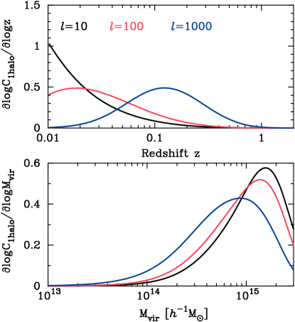
Figure 2: The derivative of the one-halo cross power spectrum with respect to redshifts or halo masses. The upper panel shows the redshift dependence on the integrand of the one-halo term, while the bottom is for the mass dependence. In each panel, the black, red, and blue lines represent the results for three different multipoles $\ell=10,100$, and 1000, respectively.

The amplitude of $C_{y\gamma}$ should scale with $A_{\gamma}$. Therefore, we can determine $A_{\gamma}$ with the measurement of the cross power spectrum when assuming the cosmological model and the degree of the hydrostatic mass bias $b_{\rm HSE}$. The exact value of $b_{\rm HSE}$ is still unclear even if we assume the concordance $\Lambda$CDM cosmology. Figure 3 shows the dependence on $b_{\rm HSE}$ of the cross power spectrum. We find that the shape of the power spectrum is almost unaffected by $b_{\rm HSE}$, but the amplitude shows a weak dependence of $b_{\rm HSE}$. Because a larger $b_{\rm HSE}$ leads to a smaller amplitude in the thermal pressure profile for a given halo mass $M$ [see Eq. (22)], the amplitude of the correlation is expected to decrease as $b_{\rm HSE}$ increases. This indicates that the constraint of $A_{\gamma}$ by the cross power spectrum can depend on the assumed value of $b_{\rm HSE}$. In this paper, we consider a wide range of $b_{\rm HSE}$ from 0.1 to 0.7 when constraining $A_{\gamma}$ with the measurement of the power spectrum (see Sec. V.3).

It is worth noting that there should exist other contributions to the power spectrum from the clustering faint astrophysical sources at gamma-ray and microwave wavelengths. In Appendix A, we examine the possible correlation between the main gamma-ray sources and the tSZ effect by the ICM. We find that the contribution from the gamma-ray sources would be subdominant in the power spectrum, and thus, we ignore any possible cross-correlation signals arising from astrophysical sources. Nevertheless, this treatment should provide a conservative upper limit on the parameter $A_{\gamma}$, since the correlation from the astrophysical sources is expected to be positive.

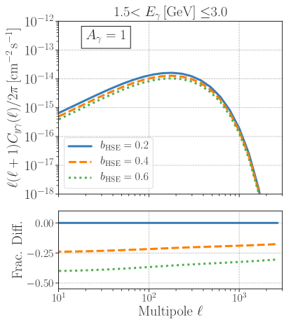
Figure 3: The dependence of the cross power spectrum on the hydrostatic mass bias. The blue solid line shows the case of $b_{\rm HSE}=0.2$ as our baseline model, while the orange dashed and green dotted lines represents the results with $b_{\rm HSE}=0.4$ and $b_{\rm HSE}=0.6$, respectively. The upper panel shows the cross power spectrum, while the bottom represents the fractional difference between the model with $b_{\rm HSE}=0.2$ and others.

IV DATA

IV.1 Fermi-LAT

The data for this study were taken during the period August 4, 2008, to August 2, 2016, covering eight years. We used the current version of LAT data which is Pass 8 and the P8R3_ULTRACLEANVETO_V2 event class. We also took advantage of a new event classification that divides the data into quartiles according to the localization quality of the events. In particular, we rejected the worst quartile denoted as PSF0. Furthermore, to reduce contamination from the Earth’s albedo, we excluded photons detected with a zenith angle larger than 90^∘. The data reduction procedure was done using version v11r5p3 of the Fermi Science Tools software package. Note that the selection cuts in our analysis are very similar to those introduced in Ref. [54]. The interested reader is referred to that article for validation tests and further checks on the data sample.

We analyzed LAT data in the energy range between 700 MeV and 1 TeV. The whole data set was subdivided into 100 logarithmically spaced “micro” energy bins. For each micro-energy bin, we produced counts and exposure maps which were subsequently used to obtain raw flux maps. The resulting maps were spatially binned using the Healpix [55] framework with $N_{\rm side}=512$. In this paper, we consider three energy bins of $0.7<E_{\gamma}\,[\rm GeV]\leq 1.5$, $1.5<E_{\gamma}\,[\rm GeV]\leq 3.0$, and $E_{\gamma}>3\,[\rm GeV]$ for cross-correlation analyses to study the gamma-ray energy dependence. We also note that the effect of the energy dependent gamma-ray PSF is properly included in the theoretical model as in Ref. [30], when we compare our model with the observed cross correlations.

IV.2 Compton-$y$ map by the Planck satellite

To perform the cross-correlation analysis, we use the publicly available tSZ Compton map provided by the Planck collaboration. The Compton $y$ map has been constructed by the component separation of the Planck full mission data covering $30$ to $857\,\mathrm{GHz}$ frequency channels [23]. The original map is provided in Healpix format with $N_{\mathrm{side}}=2048$, but we degrade the map with $N_{\mathrm{side}}=512$ to be same as in the UGRB map. Although the observed maps at multiple frequency bands have different beam properties, we assume circularly symmetric Gaussian beam with the full-width half-mean (FWHM) beam size $\theta_{\mathrm{FWHM}}=10.0\,\mathrm{arcmin}$ for the Compton-$y$ map. This Gaussian beaming effect is properly included in our theoretical model when we compare the model with the observed cross correlation. For the map production, the Planck team examined two different component separation algorithm: MILCA (Modified Internal Linear Combination Algorithm) [56] and NILC (Needlet Independent Linear Combination) [57]. Either is designed to find the linear combination of several components with optimal weight. The weight is set so that the variance of the reconstructed map is minimized. In this paper, we use the map constructed with MILCA as the fiducial map because it has lower noise contribution at large scales.

IV.3 Masking

When performing the cross-correlation analysis, we masked some regions to avoid any contamination from resolved gamma-ray point sources and imperfect modeling of Galactic gamma-ray emission. Namely, we masked all the extended and point-like sources listed in the 4FGL catalog [58]. For energies larger than 10 GeV we also masked the 3FHL catalog [59] sources. The source mask takes into account both the energy dependence of the PSF and the brightness of each source. This is the same as in Ref. [54], below we provide a brief description of the procedure proposed in that article.

For each micro-energy bin [$E\rm{{}_{i}}$, $E\rm{{}_{f}}$], we take the containment angle as given by $\rm{PSF}(E_{\rm{i}})$, which is in turn obtained as the mean of the three quartiles included in our data sample (PSF1, PSF2, PSF3). This value is subsequently used to define the radius of each source $r_{src}$. Conservatively, we take $r_{src}$ to vary from a minimum of 2$\times\rm{PSF}(E_{\rm{min}})$, for the faintest source with flux $F_{\rm{min}}$, to a maximum $F_{\rm{max}}$ of 5$\times\rm{PSF(E_{i})}$, for the brightest one. For sources with $F_{\rm{src}}$ somewhere in between these two extremes, we use a logarithmic scaling of the form [54]:

$$\frac{r_{\rm{src}}(F_{\rm{src}},E_{\rm{i}})-2\times\rm{PSF}(E_{\rm{i}})}{5\times\rm{PSF}(E_{\rm{i}})-2\times\rm{PSF}(E_{\rm{i}})}=\frac{\log(F_{\rm{src}})-\log(F_{\rm{min}})}{\log(F_{\rm{max}})-\log(F_{\rm{min}})}$$

As done in Ref. [54], we also kept E_min=8.3 GeV for micro energy bins above 14.5 GeV.

We removed the Galactic diffuse emission (GDE) using the most up-to-date foreground emission model gll_iem_v07.fits. For this, we ran maximum likelihood fits in each micro-energy bin in which the flux normalization for the GDE model was free to vary. We also floated in the fits the normalization of an isotropic emission model (iso_P8R3_ULTRACLEANVETO_V2_v1.txt) accounting for the UGRB and possible cosmic-ray residuals in the data. Given that we are using the same amount of data used in the construction of the 4FGL catalog, it is well justified to fix all 4FGL point sources to their catalog values in the fitting procedure. The fits were performed with the pylikelihood routine within the Fermi Science Tools, which now provide support for likelihood analyses using maps in Healpix projection. In agreement with results in Ref. [54], we found normalizations for the GDE that are within $1\sigma$ statistical uncertainty of the canonical values. Using our best-fit GDE model values, we constructed infinite-statistics model maps with the gtmodel tool in each energy bin. These were then subtracted from the raw flux maps. We applied the point source mask after this step to obtain the final UGRB maps.

As shown in Figure 2, the ICM in low-$z$ galaxy clusters can affect the large-scale amplitude of the cross power spectrum. To make our correlation analysis self-consistent, we apply circular masks around three nearby galaxy clusters at $z<0.01$. Those includes Virgo, Fornax, and Antlia clusters. We set the mask radius to be 8.0, 8.0 and 3.6 degree for Virgo, Fornax, and Antlia, respectively. Note that these masks can cover the area beyond the virial region of individual nearby clusters [60].

For the microwave sky, we mask Galactic planes and point sources, where strong radio emission component separation becomes unreliable. We employ the 60% Galactic mask and point source mask provided by Planck collaboration. After placing the masks in the UGRB map at different gamma-ray energy bins, the sky coverage fraction of our data region is 11.1%, 18.1% and 22.1% for the energy range of $0.7<E_{\gamma}\,[\rm GeV]\leq 1.5$, $1.5<E_{\gamma}\,[\rm GeV]\leq 3.0$, and $E_{\gamma}\,[\rm GeV]>3.0$, respectively. Figure 4 shows our mask region used in the cross-correlation analysis for the gamma-ray energy bin of $1.5<E_{\gamma}\,[\rm GeV]\leq 3.0$, while Figure 5 shows the observed gamma-ray, the UGRB and the Compton-$y$ maps. It is worth noting that the CMB has a distinct component of diffuse Galactic emission called the Galactic “Haze”. In practice, the Haze could still remain as a residual in the Planck $y$ map as well, and it would correlate with the Fermi Bubbles appeared in the middle in Figure 5 [61]. In Appendix C, we investigate the effect of the Fermi Bubbles and the Loop I structure on our power spectrum measurements by masking the known structures. There, we conclude that neither of the Fermi Bubbles nor the Loop I structure compromises our results.

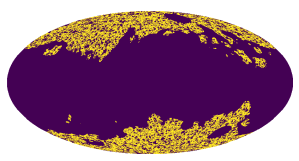
Figure 4: Fiducial mask applied in our analysis for the $1.5<E_{\gamma}\,[\rm GeV]\leq 3.0$ energy bin. Darker regions in this figure represent masks. We mask the resolved gamma-ray and radio point sources and the strong Galactic emission around the Galactic plane.

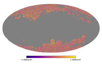
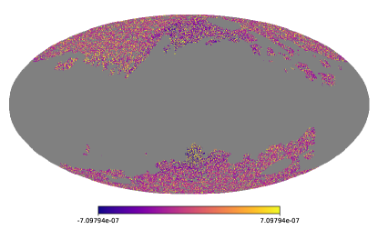
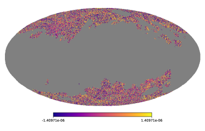
Figure 5: Gamma-ray and compton $y$ maps in our analysis. The upper map shows the gamma-ray intensity map at $1.5<E_{\gamma}\,[\rm GeV]\leq 3.0$ before the subtraction of galactic components, while the middle map represents the UGRB counterpart. The lower map is the MILCA $y$ map provided by the Planck collaboration. Note that the gamma-ray intensity has units of ${\rm cm}^{-2}\,{\rm s^{-1}}$, while the $y$ map is dimensionless. In each map, the gray region shows the masked area.

IV.4 Estimator of cross correlation

We then estimate the cross power spectrum between the Fermi UGRB map and the Planck Compton $y$ map using a pseudo-$C_{\ell}$ approach [62]. For this purpose, we make use of the publicly available tool PolSpice [63, 64]. The algorithm properly deconvolves the power spectrum from mask effects in the maps of interest, but it is known not to be a minimum variance algorithm [65]. In this sense, the associated covariance matrix is likely to overestimate the actual uncertainty, making the significance reported in this paper conservative. We first measure the power spectrum in the multipole range from $\ell=10$ to 1000. To mitigate possible mode-mixing effects caused by masks, we then average the measured power spectrum in 10 logarithmic bins with a bin width of $\Delta\ln\ell=0.46$.

The statistical uncertainty of the cross power spectrum $C_{y\gamma}$ can be decomposed into two parts. One is the common Gaussian covariance term and it is given by

$${\rm Cov}_{\rm G}[C_{y\gamma_{a}}(\ell_{1}),C_{y\gamma_{b}}(\ell_{2})] = \frac{\delta_{\ell_{1}\ell_{2}}}{(2\ell_{1}+1)\Delta\ell\,\sqrt{f_{{\rm sky},a}f_{{\rm sky},b}}}$$ (28)

$$\times\Big{[}C_{yy}(\ell_{1})C_{\gamma_{a}\gamma_{b}}(\ell_{1})$$

$$+C_{y\gamma_{a}}(\ell_{1})C_{y\gamma_{b}}(\ell_{1})\Big{]},$$

where $C_{y\gamma_{a}}$ represents the cross power spectrum between the $y$ map and the $a$-th bin in the gamma-ray energy in the UGRB map, $C_{yy}$ is the auto power spectrum of the $y$ map, $C_{\gamma_{a}\gamma_{b}}$ is the cross power spectrum between two different energy bins in the observed gamma-ray maps (including the Galactic emission), and $f_{{\rm sky},a}$ is the sky fraction of the data region used in the cross-correlation analysis at the $a$-th bin in the gamma-ray energy. Note that each term in the right hand side in Eq. (28) is measurable with the PolSpice algorithm. Also, the PolSpice calculates the the right hand side in Eq. (28) including the Poisson noise.

The PolSpice algorithm is not designed to provide the minimum-variance estimates, but the actual Gaussian covariance should be affected by the mode coupling due to sky masking [65]. The public code of PolSpice can provide the covariance matrix that take the geometric effects of mode coupling into account [66] if the gamma-ray energy bins are identical, i.e., $a=b$ in Eq. (28). Hence, we modify the Gaussian covariance term by using the covariance estimated by PolSpice as [67]

$${\rm Cov}_{\rm G,mod}[C_{y\gamma_{a}}(\ell_{1}),C_{y\gamma_{b}}(\ell_{2})]$$ (31)

$$= \left\{\begin{array}[]{ll}{\scriptstyle{\rm Cov}_{\rm P}[C_{y\gamma_{a}}(\ell_{1}),C_{y\gamma_{b}}(\ell_{2})]}&{\scriptstyle(a=b)}\\ {\scriptstyle\Gamma_{a}(\ell_{1})\Gamma_{b}(\ell_{2}){\rm Cov}_{\rm G}[C_{y\gamma_{a}}(\ell_{1}),C_{y\gamma_{b}}(\ell_{2})]}&{\scriptstyle(a\neq b)}\\ \end{array}\right.,$$

where ${\rm Cov}_{\rm P}$ is the covariance matrix provided by the PolSpice code, and the correction factor $\Gamma_{a}(\ell_{1})$ is defined as

$$\Gamma_{a}(\ell)=\left(\frac{{\rm Cov}_{\rm P}[C_{y\gamma_{a}}(\ell),C_{y\gamma_{a}}(\ell)]}{{\rm Cov}_{\rm G}[C_{y\gamma_{a}}(\ell),C_{y\gamma_{a}}(\ell)]}\right)^{1/2}.$$ (32)

Note that Eq. (31) includes the correlated scatters among different $\ell$ bins.

Another contribution to the statistical error of $C_{y\gamma}$ is the four-point correlation function in the data region, referred to as the non-Gaussian covariance. We predict this non-Gaussian term based on the halo-model approach as in Sec III. In the halo-model approach, the non-Gaussian covariance can be expressed as (e.g. see Ref. [68] for the cross-correlation between the Compton $y$ and galaxies)

$${\rm Cov}_{\rm NG}[C_{y\gamma_{a}}(\ell_{1}),C_{y\gamma_{b}}(\ell_{2})] = \frac{1}{4\pi\sqrt{f_{{\rm sky},a}f_{{\rm sky},b}}}\int\,{\rm d}z\,\frac{{\rm d}^{2}V}{{\rm d}z{\rm d}\Omega}$$ (33)

$$\times\int\,{\rm d}M\,\frac{{\rm d}n}{{\rm d}M}\,$$

$$\times y_{\ell_{1}}\gamma_{a,\ell_{1}}y_{\ell_{2}}\gamma_{b,\ell_{2}},$$

where $y_{\ell}$ and $\gamma_{\ell}$ are the Fourier transforms of the compton $y$ and the gamma-ray emissivity profiles for a single halo (see Sec III.2.3). Note that we omit the arguments of halo masses $M$ and redshifts $z$ for $y_{\ell}$ and $\gamma_{\ell}$ in Eq. (33) for simplicity. In Appendix B, we show that the non-Gaussian error can be important for our measurements of the cross power spectrum at $\ell\sim 100$.

V RESULTS

V.1 Measurements of cross power spectrum

We summarize our measurement of the cross power spectrum between the Fermi UGRB and the Planck Compton $y$ maps. Figure 6 shows the measured power spectra for three different energy bins $0.7<E_{\gamma}\,[\rm GeV]\leq 1.5$, $1.5<E_{\gamma}\,[\rm GeV]\leq 3.0$ and $E_{\gamma}\,[\rm GeV]>3.0$. The detection significance of the power spectra is commonly characterized as the signal-to-noise ratio, which is defined by

$$\left({\rm S}/{\rm N}\right)^{2} = \sum_{a,b}\sum_{i,j}{\rm Cov}^{-1}_{\rm null}(\ell_{i},\ell_{j};a,b)$$ (34)

$$\qquad\qquad\qquad\times C_{y\gamma,a}(\ell_{i})\,C_{y\gamma,b}(\ell_{j}),$$

where $C_{y\gamma,a}(\ell_{i})$ is the cross power spectrum at the multipole $\ell_{i}$ for $a$-th energy bin in the UGRB map and ${\rm Cov}_{\rm null}$ is given by Eq. (31) with $C_{y\gamma,a}=C_{y\gamma,b}=0$. Note that we set the non-Gaussian covariance to be zero in Eq. (34), because we define the significance testing a null detection.

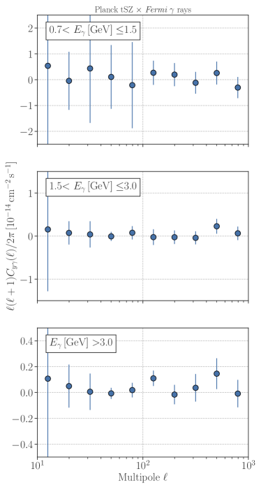
Figure 6: Measurement of cross power spectrum by varying the minimum gamma-ray energy in Fermi UGRB map.

	$10<\ell<1000$
$0.7<E_{\gamma}\,[\rm GeV]\leq 1.5$	2.59 (10)
$1.5<E_{\gamma}\,[\rm GeV]\leq 3.0$	5.02 (10)
$E_{\gamma}\,[\rm GeV]>3.0$	7.95 (10)
Combined	10.76 (30)

Table 1: Summary of the significance of our cross-correlation measurements. Second and third columns represent the $({\rm S}/{\rm N})^{2}$ defined in Eq. (34) and the numbers in brackets show the degree of freedom in the analysis.

Table 1 represents the signal-to-noise ratio of our cross-correlation measurements. We find that the power spectra at $\ell\lower 2.15277pt\hbox{$\;\buildrel<\over{\sim}\;$}100$ have larger statistical uncertainties than at high-$\ell$s. This is because the complex survey geometry induces mode coupling between different multipoles in a non-trivial manner. Once taking into account the covariance between $\ell_{1}\neq\ell_{2}$, we find that our measurement is consistent with a null detection. In Appendix C, we examine three systematic effects in our measurement of the cross power spectrum to validate the null detection: imperfect modeling of Milky-way gamma-ray foregrounds, the inaccurate reconstruction of Compton $y$, and possible large-scale correlations between Galactic gamma rays with CMB maps. In summary, we conclude that the cross power spectrum at $10<\ell<1000$ is minimally affected by these systematic uncertainties.

V.2 Comparison with halo model

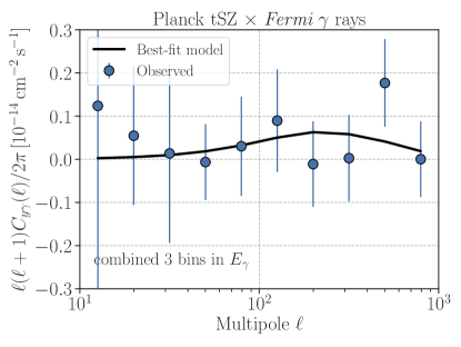
Figure 7: Comparison of the observed cross power spectrum with our best-fit model. The gray hatched region is excluded in the likelihood analysis. In this figure, we combine the power spectra with 3 bins in the gamma-ray energy by using the minimum variance weight. See the text for the detail of the weight. Note that we assume the hydrostatic mass bias to be $20\%$ in this figure.

We compare our theoretical model of the UGRB-tSZ cross power spectrum with the measured signal. Since our halo-model prediction has two parameters $A_{\gamma}$ and $b_{\rm HSE}$, we perform a likelihood analysis to find the best-fit model to the measurement. We infer the best-fit $A_{\gamma}$ to minimize the following log-likelihood for a given $b_{\rm HSE}$:

$$-2\log L = \sum_{a,b}\sum_{i,j}{\rm Cov}^{-1}_{\rm G+NG}(\ell_{i},\ell_{j};a,b;A_{\gamma})$$ (35)

$$\qquad\times\left[C^{\rm obs}_{y\gamma_{a}}(\ell_{i})-C^{\rm mod}_{y\gamma_{a}}(\ell_{i};A_{\gamma})\right]$$

$$\qquad\times\left[C^{\rm obs}_{y\gamma_{b}}(\ell_{j})-C^{\rm mod}_{y\gamma_{b}}(\ell_{j};A_{\gamma})\right],$$

where ${\rm Cov}_{\rm G+NG}$ represents the covariance matrix defined by the sum of Eqs. (31) and (33), $C^{\rm obs}$ is the measured power spectrum, and $C^{\rm mod}$ is our model prediction. In Eq. (35), the indices $a$ and $b$ run over the bins in the gamma-ray energy, while the indices $i$ and $j$ are for the bins in multipoles. Note that the covariance matrix depends on the parameter $A_{\gamma}$ (see Eq. 33), but Ref. [69] points out that parameter estimates can be biased if one considers a parameter-dependence of covariance matrix in the Gaussian likelihood by including the term of $\ln|\det{\rm Cov}|$ in Eq. (35). To account for the parameter dependence of covariance in our likelihood analysis, we follow the same procedure as in Ref. [70]. First, we infer the best-fit parameter by the likelihood analysis with covariance without the non-Gaussian term. Then, we compute the non-Gaussian covariance with the best-fit parameter and perform the likelihood analysis including the non-Gaussian covariance. We iterate this procedure until the best-fit parameter converges. As the fiducial case, we assume $b_{\rm HSE}=0.2$ in this section.

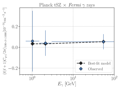
Figure 8: Similar to Fig. 7, but we compare the cross power spectrum as a function of the gamma-ray energy bin.

Figure 7 shows the comparison with the measured power spectrum and the best-fit model. In this figure, we combine the energy-dependent power spectra by using the minimum variance weight (see Ref. [71] for a similar approach). The weight is then given by

$$w_{a}(\ell)=\frac{1/{\rm Cov}_{\rm G+NG}(\ell,\ell,a,a)}{\sum_{b}1/{\rm Cov}_{\rm G+NG}(\ell,\ell,b,b)},$$ (36)

and the weighted power spectrum is defined as $C^{\rm MV}_{y\gamma}(\ell)=\sum_{a}w_{a}(\ell)\,C_{y\gamma_{a}}(\ell)$. We find the best-fit $A_{\gamma}$ to be $0.0348$ and our theoretical model can provide a reasonable fit to the observed power spectrum in the range of $10<\ell<1000$ as shown in the solid line in the figure.

Figure 8 represents our fitting result as a function of the gamma-ray energy bin. For the visualization, we show the average power spectrum over the multipole range of $100<\ell<1000$ at each of gamma-ray energy bins. The dashed line shows the best-fit model and it can explain the gamma-ray energy dependence of the measured power spectrum.

V.3 Implications for galaxy clusters

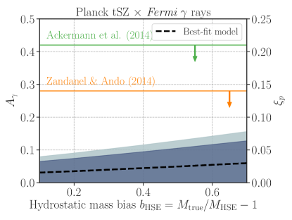
Figure 9: The comparison of our constraints on the amplitude of cosmic-ray-included gamma-ray profile $A_{\gamma}$ with respect to previous studies [11, 12]. Our constraints are shown in the blue regions. The inner region (dark blue) shows the $1\sigma$ level, while the outer one (dark grey) stands for the $2\sigma$ level. The right in the vertical axis shows the corresponding acceleration efficiency of cosmic ray protons at shocks $\xi_{p}$.

The comparisons between our model and the observed power spectrum allows us to impose constraints on $A_{\gamma}$ for a given $b_{\rm HSE}$. Our likelihood analysis yields the following 2$\sigma$-level constraints for three values of $b_{\rm HSE}$,

$$A_{\gamma} < 0.0792\,\,(b_{\rm HSE}=0.1),$$ (37)

$$A_{\gamma} < 0.0904\,\,(b_{\rm HSE}=0.2),$$ (38)

$$A_{\gamma} < 0.102\,\,(b_{\rm HSE}=0.3).$$ (39)

These constraints indicate that the acceleration efficiency of cosmic ray protons at shocks will be smaller than $\sim 5\%$. Figure 9 summarizes the constraint on $A_{\gamma}$ as a function of $b_{\rm HSE}$ and compares our constraints with previous ones. For the comparison with constraints obtained in previous works, we use Refs. [11] and [12]. The former performed a joint likelihood analysis searching for spatially extended gamma-ray emission at the locations of 50 galaxy clusters in four years of Fermi-LAT data, while the latter analyzed five-year Fermi-LAT data from the Coma galaxy cluster in the energy range between 100 MeV and 100 GeV. Comparing against the constraints shown in these previous studies, we find that our cross-correlation analysis can improve the constraints on $A_{\gamma}$ by a factor of $\sim 2-3$, provided we assume the acceptable range of $b_{\rm HSE}$ in the Planck Compton-$y$ analyses [72, 73, 68].

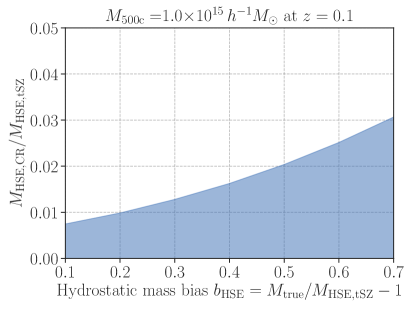
Figure 10: The $2\sigma$-level upper limits on the cosmic-ray non-thermal pressure as a function of hydro-static mass bias. To characterize the cosmic-ray-induced pressure in the model in Ref. [24], we compute the hydrostatic mass defined by the cosmic-ray pressure in the unit of the thermal-pressure counterpart. In this figure, we assume a cluster with its mass of $M_{\rm 500c}=10^{15}\,h^{-1}M_{\odot}$ at $z=0.1$. If the cosmic ray pressure is responsible to the observed hydrostatic mass bias $b_{\rm HSE}\sim 0.3$, the quantity in the vertial axis should be close to $b_{\rm HSE}$.

The constraints on $A_{\gamma}$ in Figure 9 can convert the upper limit of the amount of non-thermal pressure induced by cosmic ray protons. For a given galaxy cluster with the mass $M$ at the redshift $z$, the cosmic-ray-induced pressure can be expressed as $P_{\rm CR}(R)\propto A_{\gamma}C_{\gamma}(R)\,\rho_{\rm gas}(R)$ in the universal cosmic-ray model [24], while the thermal electron pressure $P_{e}(R)$ is given by Eqs. (22) and (23). Thus, one can formally derive the hydrostatic mass using either $P_{\rm CR}$ or $P_{e}$. Figure 10 shows the ratio of the hydrostatic mass defined by the cosmic-ray pressure and the thermal-pressure counterpart for the cluster mass $M_{\rm 500c}=10^{15}\,h^{-1}M_{\odot}$ at $z=0.1$. This figure shows that the cosmic-ray contribution to the cluster mass estimate should be smaller than the 1–3% of the commonly-used hydrostatic mass by the thermal pressure for a wide range of $b_{\rm HSE}$. This suggests that the cosmic-ray pressure can introduce only a $\lower 2.15277pt\hbox{$\;\buildrel<\over{\sim}\;$}1\%$ level of the mass bias if one adopts the total hydrostatic mass bias to be $b_{\rm HSE}\sim 0.3$.

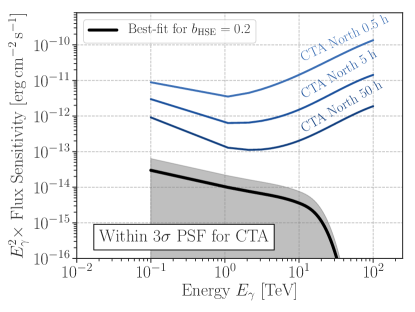
Figure 11: The expected gamma-ray flux from the Perseus cluster by our model and comparison with the flux limit in the CTA experiment. In this figure, we consider the gamma-ray flux within the $3\sigma$-level PSF radius. For the model prediction, we set $A_{\gamma}=0.0348$ assuming the hydrostatic mass bias $b_{\rm HSE}=0.2$. The gray region represents the $1\sigma$ statistical uncertainty inferred by our cross correlation analysis.

Finally, we study the detectability of the cosmic-ray-induced gamma rays from a nearby galaxy cluster with the upcoming ground-based experiment by The Cherenkov Telescope Array (CTA). As discussed in Ref. [74], the Perseus cluster is thought to be the best target for the detection of gamma rays by CTA. This is because the Perseus has a high ICM density at its center as well as it hosts the brightest radio mini-halo [75, 76].

The pion-decay-induced gamma-ray flux within the radius $R_{\theta}$ from a galaxy cluster is calculated by

$$F(>E_{\gamma,{\rm min}}) = \frac{1}{D^{2}_{L}}\int_{E_{\gamma,{\rm min}}}^{\infty}\frac{{\rm d}E_{\gamma}}{4\pi}\,\frac{{\cal S}(E^{\prime}_{\gamma},z)}{(1+z)^{3}}\,e^{-\tau(E^{\prime}_{\gamma},z(\chi))}$$ (40)

$$\qquad\times\int_{0}^{R_{\theta}}\,2\pi R_{\perp}\,{\rm d}R_{\perp}\,$$

$$\qquad\times\int_{-\infty}^{\infty}{\rm d}R_{\parallel}\,{\cal F}_{h}(R,M,z),$$

where $R=\sqrt{R^{2}_{\perp}+R^{2}_{\parallel}}$, $D_{L}$ is the luminosity distance, $E^{\prime}_{\gamma}=(1+z)E_{\gamma}$, the energy spectrum ${\cal S}$ and the gamma-ray spatial distribution ${\cal F}_{h}$ are summarized in Section III.2. For the Perseus cluster, we assume its redshift to be 0.0183 and we adopt the model of the electron density constrained by the X-ray observation [77]. We also set the mass of the Perseus cluster by 1.2 times the hydrostatic mass obtained in Ref. [77] (i.e. we assume $b_{\rm HSE}=0.2$). From the electron density $n_{e}$, we compute the gas density by $\rho_{\rm gas}=m_{p}n_{e}/(X_{H}X_{e})$. To be conservative, we here ignore the gas clumpiness effect for the model prediction (i.e. $C_{\rm clump}=1$).

Figure 11 shows our model prediction of the gamma-ray flux from the Perseus cluster and the comparison with the expected flux limit by the CTA experiment. The blue lines in the figure represent the flux limits as a function of the observational time, while the solid line is the prediction by our best-fit model. According to a simple extrapolation, we expect that the flux limit with a 500-hour observation will be comparable to the expected cosmic-ray induced gamma rays from the Perseus at $E_{\gamma,{\rm min}}\sim 1\,{\rm TeV}$. It would be worth noting that our model does not include the contribution from gamma-ray point sources in the Perseus cluster. To detect the ICM-induced gamma rays, one need to subtract the non-ICM contribution from real data as well. We leave investigations into more realistic gamma-ray analyses for future studies.

V.4 Halo Model Uncertainties

Our model based on the halo-model approach relies on several assumptions. To assess the model uncertainties of the tSZ-URGB power spectrum, we consider four important elements in our model, and examine the variations and uncertainties associated with them. Figure 12 summarizes our findings. In short, the cosmological parameters can cause a $\pm$30%-level uncertainty, while the fitting function of the gamma-ray emission profile in Ref. [24] and the gas clumpiness affect our modeling by $\pm$20%. The detailed shape of the cluster pressure profile is found to be negligible for the current analysis. Hence, the total uncertainty in our model can amount up to $30+20+20=70\%$. However, even considering the maximal $\pm$70%-level uncertainty, we find that our constraint of $A_{\gamma}$ in Fig. 9 is still tighter than previous limits.

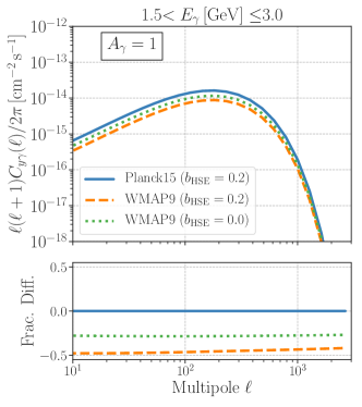
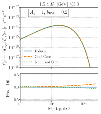
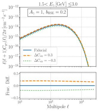
Figure 12: Modeling uncertainties of the tSZ-UGRB cross power spectrum. In every panel, the upper portion shows power spectra in the gamma-ray energy range of 1.5-3.0 GeV with different model parameters, and the bottom potion shows the fractional difference to our fiducial model. Top left: The cosmological dependence. The blue line shows our fiducial model assuming the Planck15 cosmology and the hydrostatic mass bias $b_{\rm HSE}=0.2$, while the orange dashed line shows the model assuming the WMAP9 cosmology with $b_{\rm HSE}=0.2$. The green dotted line presents the model assuming the WMAP9 cosmology with $b_{\rm HSE}=0.0$, which is consistent with the recent constraint of cosmology and $b_{\rm HSE}$ inferred from the tSZ auto power spectrum in the Planck [73]. Top right: The dependence on the shape of ICM pressure profiles. The blue line shows our fiducial model, while the orange dashed and green dotted lines assume the pressure profiles for cool-core and non cool-core clusters, respectively. The parameters of the pressure profiles are taken from Ref. [49]. Bottom left: The dependence on a parameter in gamma-ray profiles in PP10. We vary the amplitude of the mass-dependent term in the gamma-ray profiles (Eq. 13 or $C_{\rm vir}$) by $\pm 30\%$. Bottom right: The dependence on gas clumpiness. The blue line shows our fiducial model, while the orange dashed line represents the model without the effect of gas clumpiness.

V.4.1 Cosmological dependence

The abundance of cluster-sized dark matter halos strongly depends on cosmological parameters [3]. Therefore, the assumed cosmology can affect our modeling of the tSZ-UGRB power spectrum. For our fiducial model, we adopt the cosmological parameters inferred from the CMB power spectra measured by Planck [78]. We refer this cosmological model as Planck15. For comparison, we also adopt the cosmological parameters constrained by the WMAP nine-year (WMAP9) data [79]. By assuming a reasonable value for hydrostatic mass bias $b_{\rm HSE}=0.2$, we find that the model based on the WMAP9 cosmology can differ from our fiducial model by a factor of 0.5. However, this comparison does not take into account another important constraint by the tSZ auto power spectrum. The tSZ auto power spectrum can constrain the combination of cosmological parameters and $b_{\rm HSE}$ as $\sigma_{8}\,[\Omega_{\rm m0}/(1+b_{\rm HSE})]^{0.4}\,h^{-0.21}$ [73]. To make the amplitude of the tSZ power spectrum consistent between Planck15 and WMAP9 models, we find that $b_{\rm HSE}=0.0$ is required for the WMAP9 model. When adding the prior information about cosmology and $b_{\rm HSE}$ expected from the tSZ power spectrum, we find that the WMAP9-based model is smaller than our fiducial model at a level of 30%. Hence, we conclude that the current cosmological uncertainties can induce a $\pm$30%-level uncertainty in our modeling of the tSZ-UGRB power spectrum.

V.4.2 Shape of cluster pressure profile

It is known that the ICM pressure profile can depend not only on cluster mass but also other properties of individual clusters. The Planck observation of nearby galaxy clusters has found that the pressure profile varies depending on whether a cluster has a central temperature drop[49]. Clusters with central temperature drops are commonly called cool-core clusters. The parameters of the shape of pressure profiles for cool-core and non cool-core clusters have been constrained separately in Ref. [49]. We use those different parameters in modeling the tSZ-UGRB power spectrum and compare with our fiducial model. We find that the dependence of our modeling on the shape of pressure profile is small. It can induce at most a $\pm$10%-level uncertainty at $\ell\simeq 2000$. Since our likelihood analysis limits the multipole range to $10<\ell<1000$, we conclude that the modeling uncertainty associated with the pressure profile should be unimportant for the current analysis.

V.4.3 Fitting function of gamma-ray emission profiles

Our model of the tSZ-UGRB power spectrum relies on the simulation results in Ref [24]. The authors in Ref [24] use a fitting formula for the gamma-ray emission profile as a function of cluster mass and radius. Among the parameters in the fitting function, the amplitude of the mass-dependent term in the gamma-ray profile (Eq. 13 or $C_{\rm vir}$) appears to be subject to a $\pm$30%-level uncertainty (see Figure 8 in Ref [24]). We examine the impact of a $\pm$30% difference in $C_{\rm vir}$ on the modeling of the tSZ-UGRB power spectrum. We find that the $\pm$30%-level uncertainty in $C_{\rm vir}$ can change our prediction of the tSZ-UGRB power spectrum by $\pm$20%.

V.4.4 Gas clumpiness

The gas clumpiness effect (Eq. 17) can boost the expected cross power spectrum. We adopt the simulation-based model of $C_{\rm clump}$ as in Ref [47], while it has been poorly validated by actual observations. We examine the impact of gas clumpiness on our modeling and find that including the factor $C_{\rm clump}$ can increase the amplitude of the cross power spectrum by a factor of $\sim 20\%$.

VI CONCLUSION AND DISCUSSION

We studied the gamma rays induced by the cosmic ray in the ICM using a cross-correlation analysis with the unresolved extragalactic gamma-ray background (UGRB) and the thermal Sunyaev-Zel’dovich (tSZ) effect in the cosmic microwave background. We developed a theoretical model of the cross-correlation signal based on the cosmic-ray model calibrated by the hydrodynamical simulation [24]. We found that the cross power spectrum at the multipole $\ell\sim 1000$ (or the equivalent angular scale being $\sim 10\,{\rm arcmin}$) contains the information on the cosmic-ray-induced gamma rays from the galaxy clusters outside the local Universe at $z=0.1$–0.2, while clusters at $z<0.1$ are responsible for the signals at $\ell\sim 100$.

We also measured the cross power spectrum for the first time by using eight years of Fermi gamma-ray data and the publicly available tSZ map by Planck. Our measurement is consistent with a null detection. Comparing the observed power spectra with our theoretical model, we impose constraints on the acceleration efficiency of cosmic ray protons at shocks around the most massive objects in the Universe. Our cross-correlation analysis sets the $2\sigma$-level upper limits of the acceleration efficiency to be $\sim 7.8\%$. This constraint is more stringent than previous ones [11, 12] by a factor of $\sim 2-3$, while it is consistent with recent numerical studies [80, 81, 82].

Our constraint of the acceleration efficiency implies that the cosmic-ray pressure cannot be responsible for the observed hydrostatic mass bias in the tSZ-selected clusters [72]. We expect that the cosmic rays in the ICM will introduce a $\sim 1\%$-level of the hydrostatic mass bias at most and it is smaller than the current limits of the hydrostatic mass bias (e.g. see Refs [72, 73, 68]). Besides, we studied the future detectability of the pion-decay-induced gamma rays from the Perseus cluster with the upcoming CTA experiment. Assuming the best-fit model to our cross-correlation measurement, we found a 500-hour observation with the CTA will be required to detect the gamma rays at the energy of $\sim 1$ TeV from the Perseus.

Our first measurement of the cross power spectra can be further improved with the future ground-based CMB experiments [83], allowing to detect the cross power spectrum at $\ell\sim 1000$ with a high significance level. Such a precise measurement can reveal the nature of energetic components in the ICM as well as the physics of active Galactic nuclei (AGN) inside galaxy clusters. Although our analysis ignores possible angular correlations caused by any astrophysical sources, it will become more important to understand the future precise measurement. A joint cross-correlation analysis among multi-wavelength data is one of the interesting approaches to constrain the nature of ICM as well as properties of any faint astronomical sources (e.g. see Ref. [84] for the ICM and Ref. [85] for the astrophysical sources). Future studies should focus on the development of accurate modeling of the ICM and astrophysical sources and optimal design of multi-wavelength data analysis.

Appendix A CROSS CORRELATION CAUSED BY GAMMA RAYS FROM ASTRONOMICAL OBJECTS

Figure 13: The expected contribution to the cross power spectrum from the clustering of faint blazars and misaligned AGNs (mAGNs). The dashed line shows the signal caused by the blazars, while the gray solid line represents the expected correlation with the mAGNs. For reference, the solid line shows the best-fit model of the cosmic-ray-induced signal to our power-spectrum measurement. In this figure, we included the beaming effect in the Planck compton $y$ map.

In the main text, we ignore possible correlations arising from the clustering of faint astrophysical sources which cannot be resolved on an individual basis. Among various astrophysical sources at gamma rays and microwave, blazars and misaligned AGNs (mAGNs) are expected to be potentially important in our analysis. This is because faint blazar populations can be responsible for the UGRB at gamma-ray energies larger than $\sim 10$ GeV, while mAGNs can contribute significantly to the UGRB at $\sim 1$ GeV [86]. Also, blazars and mAGNs likely reside in massive dark matter halos (e.g., Refs [87, 88, 89]). The star forming activity in clusters can be a source of gamma rays in principle [90], however we ignore this contribution in this paper. This is because galaxy clusters are known to have quenched star forming activity (e.g., see Ref. [91]).

To evaluate the correlation between the gamma-ray emission from blazars and the tSZ effect by the ICM, we adopt the blazar model in Ref. [89]. In this model, the blazar is assumed to be a point source and located at the center of a dark matter halo. We also assume that each dark matter halo has at most one blazar. The blazar gamma-ray luminosity function and the energy spectrum have been calibrated to the existing catalog of resolved gamma-ray blazars [86]. We relate the gamma-ray luminosity of single blazars to their host halo mass by using a simple power-law model [92]. The normalization and power-law index in the mass-luminosity relation have been determined so that the model can explain the abundance of X-ray selected AGNs [93]. We convert the gamma-ray luminosity to its X-ray counterpart following Ref. [94].

For mAGNs, we adopt the model of Ref. [95], where the authors established a correlation between the gamma-ray luminosity and the radio-core luminosity $L_{r,\rm core}$ at 5 GHz. Using the correlation together with the radio luminosity function of Ref. [96], we evaluate the gamma-ray luminosity function of mAGNs. As for blazars, we assume that mAGN are point sources residing in the center of dark matter halos, and that each dark matter halo can host at most a single mAGN. We assume the mass-luminosity relation for mAGNs given in Ref. [92]. To exclude blazars and mAGNs resolved by the Fermi telescope, we impose a flux cut at $E_{\gamma}>100\,{\rm MeV}$ of $2\times 10^{-9}\,{\rm cm}^{-2}\,{\rm s}^{-1}$ in the model. For details of our models for blazars and mAGNs, we refer the reader to Refs. [92, 89, 26].

Figure 13 shows the expected cross power spectrum between the gamma-ray emission from blazars and mAGNs and the tSZ effect by the ICM. In the figure, we consider gamma-ray data in the energy bin $1.5<E_{\gamma}\,[{\rm GeV}]\leq 3.0$. The solid line represents the best-fit model of the cross power spectrum by cosmic rays in the ICM to our measurement (see Section V.1), while the dashed and gray lines are for the contribution from blazars and mAGNs, respectively. As seen in this figure, the contribution of the faint blazars and mAGNs to the UGRB-tSZ power spectrum is expected to be subdominant. This is because the tSZ signal mostly comes from the most massive galaxy clusters (e.g., see Figure 2), whereas faint astronomical objects would be mostly populated by smaller group-sized halos [87, 88].

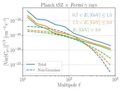
Figure 14: The statistical uncertainty in our measurement of the cross power spectrum. The solid line shows the statistical error including the non-Gaussian contribution, while the dashed one highlights the non-Gaussian error alone. The blue, orange, and green lines stand for the analyses with $0.7<E_{\gamma}\,[\rm GeV]\leq 1.5$, $1.5<E_{\gamma}\,[\rm GeV]\leq 3.0$, and $E_{\gamma}\,[\rm GeV]>3.0$, respectively.

Appendix B STATISTICAL UNCERTAINTY OF UGRB-TSZ CROSS CORRELATION

In this appendix, we show the effect of the non-Gaussian covariance in the UGRB-tSZ cross power spectrum, which is defined by Eq. (33). Figure 14 shows the diagonal elements of the covariance matrix. The dashed line shows the non-Gaussian contribution arising from the four-point correlations in the data region. In this figure, we set $A_{\gamma}=0.0348$ and $b_{\rm HSE}=0.2$. We find that the non-Gaussian error is subdominant in the diagonal elements of the covariance in the range of $\ell\lower 2.15277pt\hbox{$\;\buildrel>\over{\sim}\;$}100$, while it can become comparable to the conventional Gaussian error at $\ell\sim 100$.

Appendix C SYSTEMATIC UNCERTAINTY OF UGRB-TSZ CROSS CORRELATION

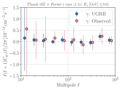
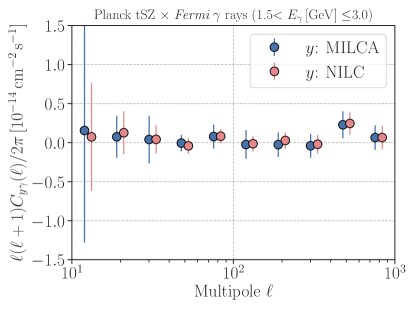
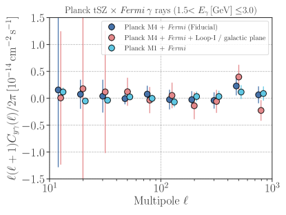
Figure 15: Dependence of the power spectrum measurement on subtraction of Galactic gamma-ray components, difference in component separation methods in CMB, and details of masks. Top left: The impact of inaccurate subtraction of Galactic components in the gamma-ray data. The blue points show our fiducial analysis, while the red ones are for the analysis without the subtraction of Galactic gamma rays. Top right: The impact of the detail of the component separation in the CMB data. The blue points show our fiducial analysis, while the red points are the results based on the tSZ map based on another approach. Bottom: The masking effect of the power spectrum analysis. The blue shows the fiducial case, while the red points show the results with masking the Fermi Bubble and Loop-I regions as well as the conservative mask around the Galactic plane. The cyan points represent the most aggressive analysis based on the 40% Galactic and point-source masks in the CMB.

In this appendix, we investigate some systematic uncertainties in the measurement of the UGRB-tSZ power spectrum. We examine three analyses below:

1. We perform the cross-correlation analysis by using the observed gamma-ray intensity. This analysis can validate the effect of the subtraction of Galactic gamma rays in the power spectrum analysis.

2. We measure the power spectrum with the UGRB map and the tSZ map based on the NILC method. This analysis will be useful to check if our measurement is sensitive to the detail of the component separation in the CMB.

3. We measure the power spectrum with the UGRB map and the fiducial tSZ map (based on the MILCA method), but we change the masked regions. We examine three cases of masking: (C1) our fiducial mask, (C2) the 60% Galactic/point source mask in the CMB and the masking around the gamma-ray sources, the Fermi Bubble and Loop-I regions with a conservative mask of $|b|<30^{\circ}$ about the Galactic plane, and (C3) the 40% Galactic/point source mask in the CMB and the masking around the gamma-ray sources. On the mask (C2), we apply a Galactic longitude cut with $0^{\circ}<\ell<50^{\circ}$ and $260^{\circ}<\ell<360^{\circ}$ to exclude the Fermi Bubble and Loop-I regions. The mask (C3) would lead to the most aggressive analysis with the largest sky coverage, but it will be most affected by the contamination due to any point sources or/and the large-scale residual Galactic emission.

Figure 15 summarizes the results of our systematic test. The left top panel shows the analysis testing the impact of Galactic gamma rays (case A), the right top panel represents the effect of the detail in the component separation in the microwave data (case B), and the bottom panel highlights the masking effect on the power spectrum analysis (case C). These analyses indicate that our measurement of the power spectrum at $10<\ell<1000$ is less affected by systematic uncertainties due to the imperfect estimates of Galactic gamma rays and the tSZ effect, the residual contribution from astrophysical sources, and a possible large-scale correlation between gamma-ray and microwave observations.

References

- Kravtsov and Borgani [2012] A. V. Kravtsov and S. Borgani, ARA&A 50, 353 (2012), arXiv:1205.5556 [astro-ph.CO] .
- Brunetti and Jones [2014] G. Brunetti and T. W. Jones, Int. J. Mod. Phys. D23, 1430007 (2014), arXiv:1401.7519 [astro-ph.CO] .
- Allen et al. [2011] S. W. Allen, A. E. Evrard, and A. B. Mantz, ARA&A 49, 409 (2011), arXiv:1103.4829 [astro-ph.CO] .
- Ferrari et al. [2008] C. Ferrari, F. Govoni, S. Schindler, A. M. Bykov, and Y. Rephaeli, Space Sci. Rev. 134, 93 (2008), arXiv:0801.0985 [astro-ph] .
- Aharonian et al. [2009] F. Aharonian et al. (HESS), A&A 502, 437 (2009), arXiv:0907.0727 [astro-ph.CO] .
- Ackermann et al. [2010] M. Ackermann et al. (Fermi-LAT), Astrophys. J. 717, L71 (2010), arXiv:1006.0748 [astro-ph.HE] .
- Ando and Nagai [2012] S. Ando and D. Nagai, J. Cosmology Astropart. Phys. 2012, 017 (2012), arXiv:1201.0753 [astro-ph.HE] .
- Arlen et al. [2012] T. Arlen et al. (VERITAS), Astrophys. J. 757, 123 (2012), arXiv:1208.0676 [astro-ph.HE] .
- Han et al. [2012] J. Han, C. S. Frenk, V. R. Eke, L. Gao, S. D. M. White, A. Boyarsky, D. Malyshev, and O. Ruchayskiy, Mon. Not. Roy. Astron. Soc. 427, 1651 (2012), arXiv:1207.6749 [astro-ph.CO] .
- Huber et al. [2013] B. Huber, C. Tchernin, D. Eckert, C. Farnier, A. Manalaysay, U. Straumann, and R. Walter, Astron. Astrophys. 560, A64 (2013), arXiv:1308.6278 [astro-ph.HE] .
- Ackermann et al. [2014] M. Ackermann et al. (Fermi-LAT), Astrophys. J. 787, 18 (2014), arXiv:1308.5654 [astro-ph.HE] .
- Zandanel and Ando [2014] F. Zandanel and S. Ando, Mon. Not. Roy. Astron. Soc. 440, 663 (2014), arXiv:1312.1493 [astro-ph.HE] .
- Ackermann et al. [2016] M. Ackermann et al. (Fermi-LAT), Astrophys. J. 819, 149 (2016), [Erratum: Astrophys. J.860,no.1,85(2018)], arXiv:1507.08995 [astro-ph.HE] .
- Ahnen et al. [2016] M. L. Ahnen et al. (MAGIC), Astron. Astrophys. 589, A33 (2016), arXiv:1602.03099 [astro-ph.HE] .
- Xi et al. [2018] S.-Q. Xi, X.-Y. Wang, Y.-F. Liang, F.-K. Peng, R.-Z. Yang, and R.-Y. Liu, Phys. Rev. D98, 063006 (2018), arXiv:1709.08319 [astro-ph.HE] .
- Zeldovich and Sunyaev [1969] Y. B. Zeldovich and R. A. Sunyaev, Ap&SS 4, 301 (1969).
- Sunyaev and Zeldovich [1972] R. A. Sunyaev and Y. B. Zeldovich, Comments on Astrophysics and Space Physics 4, 173 (1972).
- Akrami et al. [2018a] Y. Akrami et al. (Planck), (2018a), arXiv:1807.06205 [astro-ph.CO] .
- Ade et al. [2014a] P. A. R. Ade et al. (Planck), Astron. Astrophys. 571, A12 (2014a), arXiv:1303.5072 [astro-ph.CO] .
- Adam et al. [2016] R. Adam et al. (Planck), Astron. Astrophys. 594, A9 (2016), arXiv:1502.05956 [astro-ph.CO] .
- Akrami et al. [2018b] Y. Akrami et al. (Planck), (2018b), arXiv:1807.06208 [astro-ph.CO] .
- Ade et al. [2014b] P. A. R. Ade et al. (Planck), Astron. Astrophys. 571, A21 (2014b), arXiv:1303.5081 [astro-ph.CO] .
- Aghanim et al. [2016] N. Aghanim et al. (Planck), Astron. Astrophys. 594, A22 (2016), arXiv:1502.01596 [astro-ph.CO] .
- Pinzke and Pfrommer [2010] A. Pinzke and C. Pfrommer, Mon. Not. Roy. Astron. Soc. 409, 449 (2010), arXiv:1001.5023 [astro-ph.CO] .
- Branchini et al. [2017] E. Branchini, S. Camera, A. Cuoco, N. Fornengo, M. Regis, M. Viel, and J.-Q. Xia, Astrophys. J. Suppl. 228, 8 (2017), arXiv:1612.05788 [astro-ph.CO] .
- Hashimoto et al. [2018] D. Hashimoto, A. J. Nishizawa, M. Shirasaki, O. Macias, S. Horiuchi, H. Tashiro, and M. Oguri 10.1093/mnras/stz321 (2018), arXiv:1805.08139 [astro-ph.CO] .
- Colavincenzo et al. [2019] M. Colavincenzo, X. Tan, S. Ammazzalorso, S. Camera, M. Regis, J.-Q. Xia, and N. Fornengo, (2019), arXiv:1907.05264 [astro-ph.CO] .
- Gilmore et al. [2012] R. Gilmore, R. Somerville, J. Primack, and A. Dominguez, Mon.Not.Roy.Astron.Soc. 422, 3189 (2012), arXiv:1104.0671 [astro-ph.CO] .
- Abdollahi et al. [2018] S. Abdollahi et al. (Fermi-LAT), Science 362, 1031 (2018), arXiv:1812.01031 [astro-ph.HE] .
- Shirasaki et al. [2014] M. Shirasaki, S. Horiuchi, and N. Yoshida, Phys. Rev. D90, 063502 (2014), arXiv:1404.5503 [astro-ph.CO] .
- Fixsen [2009] D. J. Fixsen, ApJ 707, 916 (2009), arXiv:0911.1955 .
- Itoh et al. [1998] N. Itoh, Y. Kohyama, and S. Nozawa, ApJ 502, 7 (1998), astro-ph/9712289 .
- Chluba et al. [2012] J. Chluba, D. Nagai, S. Sazonov, and K. Nelson, Mon. Not. Roy. Astron. Soc. 426, 510 (2012), arXiv:1205.5778 .
- Hill and Pajer [2013] J. C. Hill and E. Pajer, Phys. Rev. D 88, 063526 (2013), arXiv:1303.4726 [astro-ph.CO] .
- Cooray and Sheth [2002] A. Cooray and R. Sheth, Phys. Rep. 372, 1 (2002), arXiv:astro-ph/0206508 [astro-ph] .
- Komatsu and Kitayama [1999] E. Komatsu and T. Kitayama, ApJ 526, L1 (1999), arXiv:astro-ph/9908087 [astro-ph] .
- Komatsu and Seljak [2002] E. Komatsu and U. Seljak, Mon. Not. Roy. Astron. Soc. 336, 1256 (2002), arXiv:astro-ph/0205468 [astro-ph] .
- Bryan and Norman [1998] G. L. Bryan and M. L. Norman, ApJ 495, 80 (1998), arXiv:astro-ph/9710107 [astro-ph] .
- Ade et al. [2016a] P. A. R. Ade et al. (Planck), Astron. Astrophys. 594, A27 (2016a), arXiv:1502.01598 [astro-ph.CO] .
- Tinker et al. [2008] J. Tinker, A. V. Kravtsov, A. Klypin, K. Abazajian, M. Warren, G. Yepes, S. Gottlöber, and D. E. Holz, ApJ 688, 709 (2008), arXiv:0803.2706 .
- Tinker et al. [2010] J. L. Tinker, B. E. Robertson, A. V. Kravtsov, A. Klypin, M. S. Warren, G. Yepes, and S. Gottlöber, ApJ 724, 878 (2010), arXiv:1001.3162 .
- Hu and Kravtsov [2003] W. Hu and A. V. Kravtsov, Astrophys. J. 584, 702 (2003), arXiv:astro-ph/0203169 [astro-ph] .
- Diemer and Kravtsov [2015] B. Diemer and A. V. Kravtsov, Astrophys. J. 799, 108 (2015), arXiv:1407.4730 [astro-ph.CO] .
- Sarazin [1988] C. L. Sarazin, Cambridge Astrophysics Series, Cambridge: Cambridge University Press, 1988 (1988).
- Kaiser [1986] N. Kaiser, Mon. Not. Roy. Astron. Soc. 222, 323 (1986).
- Zandanel et al. [2014] F. Zandanel, C. Pfrommer, and F. Prada, Mon. Not. Roy. Astron. Soc. 438, 116 (2014), arXiv:1311.4793 [astro-ph.CO] .
- Battaglia et al. [2015] N. Battaglia, J. R. Bond, C. Pfrommer, and J. L. Sievers, Astrophys. J. 806, 43 (2015), arXiv:1405.3346 [astro-ph.CO] .
- Lakey and Huffenberger [2019] V. Lakey and K. Huffenberger, (2019), arXiv:1902.08268 [astro-ph.CO] .
- Ade et al. [2013a] P. A. R. Ade et al. (Planck), A&A 550, A131 (2013a), arXiv:1207.4061 .
- Nagai et al. [2007] D. Nagai, A. V. Kravtsov, and A. Vikhlinin, Astrophys. J. 668, 1 (2007), arXiv:astro-ph/0703661 [astro-ph] .
- Dolag et al. [2016] K. Dolag, E. Komatsu, and R. Sunyaev, Mon. Not. Roy. Astron. Soc. 463, 1797 (2016), arXiv:1509.05134 [astro-ph.CO] .
- Ackermann et al. [2015] M. Ackermann et al. (Fermi-LAT), Astrophys. J. 812, 159 (2015), arXiv:1510.00004 [astro-ph.HE] .
- Lisanti et al. [2018] M. Lisanti, S. Mishra-Sharma, N. L. Rodd, B. R. Safdi, and R. H. Wechsler, Phys. Rev. D97, 063005 (2018), arXiv:1709.00416 [astro-ph.CO] .
- Ackermann et al. [2018] M. Ackermann et al. (Fermi-LAT), Phys. Rev. Lett. 121, 241101 (2018), arXiv:1812.02079 [astro-ph.HE] .
- Gorski et al. [2005] K. M. Gorski, E. Hivon, A. J. Banday, B. D. Wandelt, F. K. Hansen, M. Reinecke, and M. Bartelman, Astrophys. J. 622, 759 (2005), arXiv:astro-ph/0409513 [astro-ph] .
- Hurier et al. [2013] G. Hurier, J. F. Macías-Pérez, and S. Hildebrandt, A&A 558, A118 (2013), arXiv:1007.1149 [astro-ph.IM] .
- Remazeilles et al. [2011] M. Remazeilles, J. Delabrouille, and J.-F. Cardoso, Mon. Not. Roy. Astron. Soc. 410, 2481 (2011), arXiv:1006.5599 [astro-ph.CO] .
- Abdollahi et al. [2019] S. Abdollahi et al. (Fermi-LAT), (2019), arXiv:1902.10045 [astro-ph.HE] .
- Ajello et al. [2017] M. Ajello et al. (Fermi-LAT), Astrophys. J. Suppl. 232, 18 (2017), arXiv:1702.00664 [astro-ph.HE] .
- Fouque et al. [2001] P. Fouque, J. M. Solanes, T. Sanchis, and C. Balkowski, Astron. Astrophys. 375, 770 (2001), arXiv:astro-ph/0106261 [astro-ph] .
- Ade et al. [2013b] P. A. R. Ade et al. (Planck), A&A 554, A139 (2013b), arXiv:1208.5483 [astro-ph.GA] .
- Hivon et al. [2002] E. Hivon, K. M. Gorski, C. B. Netterfield, B. P. Crill, S. Prunet, and F. Hansen, Astrophys. J. 567, 2 (2002), arXiv:astro-ph/0105302 [astro-ph] .
- Chon et al. [2004] G. Chon, A. Challinor, S. Prunet, E. Hivon, and I. Szapudi, Mon. Not. Roy. Astron. Soc. 350, 914 (2004), arXiv:astro-ph/0303414 [astro-ph] .
- Szapudi et al. [2000] I. Szapudi, S. Prunet, D. Pogosyan, A. S. Szalay, and J. R. Bond, (2000), arXiv:astro-ph/0010256 [astro-ph] .
- Efstathiou [2004] G. Efstathiou, Mon. Not. Roy. Astron. Soc. 349, 603 (2004), arXiv:astro-ph/0307515 [astro-ph] .
- Challinor and Chon [2005] A. Challinor and G. Chon, Mon. Not. Roy. Astron. Soc. 360, 509 (2005), arXiv:astro-ph/0410097 [astro-ph] .
- Fornengo et al. [2015] N. Fornengo, L. Perotto, M. Regis, and S. Camera, Astrophys. J. 802, L1 (2015), arXiv:1410.4997 [astro-ph.CO] .
- Makiya et al. [2018] R. Makiya, S. Ando, and E. Komatsu, Mon. Not. Roy. Astron. Soc. 480, 3928 (2018), arXiv:1804.05008 [astro-ph.CO] .
- Carron [2013] J. Carron, A&A 551, A88 (2013), arXiv:1204.4724 [astro-ph.CO] .
- Makiya et al. [2019] R. Makiya, C. Hikage, and E. Komatsu, (2019), arXiv:1907.07870 [astro-ph.CO] .
- Shirasaki et al. [2016] M. Shirasaki, O. Macias, S. Horiuchi, S. Shirai, and N. Yoshida, Phys. Rev. D94, 063522 (2016), arXiv:1607.02187 [astro-ph.CO] .
- Ade et al. [2016b] P. A. R. Ade et al. (Planck), Astron. Astrophys. 594, A24 (2016b), arXiv:1502.01597 [astro-ph.CO] .
- Bolliet et al. [2018] B. Bolliet, B. Comis, E. Komatsu, and J. F. Macías-Pérez, Mon. Not. Roy. Astron. Soc. 477, 4957 (2018), arXiv:1712.00788 [astro-ph.CO] .
- Acharya et al. [2018] B. S. Acharya et al. (CTA Consortium), Science with the Cherenkov Telescope Array (WSP, 2018) arXiv:1709.07997 [astro-ph.IM] .
- Pedlar et al. [1990] A. Pedlar, H. S. Ghataure, R. D. Davies, B. A. Harrison, R. Perley, P. C. Crane, and S. W. Unger, Mon. Not. Roy. Astron. Soc. 246, 477 (1990).
- Gitti et al. [2002] M. Gitti, G. Brunetti, and G. Setti, Astron. Astrophys. 386, 456 (2002), arXiv:astro-ph/0202279 [astro-ph] .
- Churazov et al. [2003] E. Churazov, W. Forman, C. Jones, and H. Bohringer, Astrophys. J. 590, 225 (2003), arXiv:astro-ph/0301482 [astro-ph] .
- Ade et al. [2016c] P. A. R. Ade et al. (Planck), Astron. Astrophys. 594, A13 (2016c), arXiv:1502.01589 [astro-ph.CO] .
- Hinshaw et al. [2013] G. Hinshaw et al. (WMAP), Astrophys. J. Suppl. 208, 19 (2013), arXiv:1212.5226 [astro-ph.CO] .
- Vazza et al. [2016] F. Vazza, M. Brüggen, D. Wittor, C. Gheller, D. Eckert, and M. Stubbe, Mon. Not. Roy. Astron. Soc. 459, 70 (2016), arXiv:1603.02688 [astro-ph.GA] .
- Ryu et al. [2019] D. Ryu, H. Kang, and J.-H. Ha 10.3847/1538-4357/ab3a3a (2019), arXiv:1905.04476 [astro-ph.HE] .
- Ha et al. [2019] J.-H. Ha, D. Ryu, and H. Kang, (2019), arXiv:1910.02429 [astro-ph.HE] .
- Abazajian et al. [2016] K. N. Abazajian et al. (CMB-S4), (2016), arXiv:1610.02743 [astro-ph.CO] .
- Shirasaki et al. [2019] M. Shirasaki, E. T. Lau, and D. Nagai, (2019), arXiv:1909.02179 [astro-ph.CO] .
- Shirasaki [2019] M. Shirasaki, Mon. Not. Roy. Astron. Soc. 483, 342 (2019), arXiv:1807.09412 [astro-ph.CO] .
- Ajello et al. [2015] M. Ajello et al., Astrophys. J. 800, L27 (2015), arXiv:1501.05301 [astro-ph.HE] .
- Lindsay et al. [2014] S. N. Lindsay, M. J. Jarvis, M. G. Santos, M. J. I. Brown, S. M. Croom, S. P. Driver, A. M. Hopkins, J. Liske, J. Loveday, P. Norberg, and A. S. G. Robotham, Mon. Not. Roy. Astron. Soc. 440, 1527 (2014), arXiv:1402.5654 [astro-ph.CO] .
- Allevato et al. [2014] V. Allevato, A. Finoguenov, and N. Cappelluti, Astrophys. J. 797, 96 (2014), arXiv:1410.0358 [astro-ph.GA] .
- Shirasaki et al. [2018] M. Shirasaki, O. Macias, S. Horiuchi, N. Yoshida, C.-H. Lee, and A. J. Nishizawa, Phys. Rev. D97, 123015 (2018), arXiv:1802.10257 [astro-ph.CO] .
- Storm et al. [2012] E. M. Storm, T. E. Jeltema, and S. Profumo, ApJ 755, 117 (2012), arXiv:1206.1676 [astro-ph.HE] .
- Somerville and Davé [2015] R. S. Somerville and R. Davé, ARA&A 53, 51 (2015), arXiv:1412.2712 [astro-ph.GA] .
- Camera et al. [2015] S. Camera, M. Fornasa, N. Fornengo, and M. Regis, JCAP 1506 (06), 029, arXiv:1411.4651 [astro-ph.CO] .
- Hütsi et al. [2014] G. Hütsi, M. Gilfanov, and R. Sunyaev, Astron. Astrophys. 561, A58 (2014), arXiv:1304.3717 [astro-ph.CO] .
- Inoue and Totani [2009] Y. Inoue and T. Totani, Astrophys. J. 702, 523 (2009), [Erratum: Astrophys. J.728,73(2011)], arXiv:0810.3580 [astro-ph] .
- Di Mauro et al. [2014] M. Di Mauro, F. Calore, F. Donato, M. Ajello, and L. Latronico, Astrophys. J. 780, 161 (2014), arXiv:1304.0908 [astro-ph.HE] .
- Willott et al. [2001] C. J. Willott, S. Rawlings, K. M. Blundell, M. Lacy, and S. A. Eales, Mon. Not. Roy. Astron. Soc. 322, 536 (2001), arXiv:astro-ph/0010419 [astro-ph] .