Supplemental information for:
Nature of symmetry breaking at the excitonic insulator transition: Ta₂NiSe₅

I Ab-initio Calculations

Our ab-initio calculations are performed using density functional theory (DFT) initially applying the generalized gradient approximation (GGA / PBE) Perdew et al. (1996) within the PAW formalism Blöchl (1994) as implemented in the Vienna Ab initio Simulation Package (VASP) Kresse and Furthmüller (1996a, b). We start with fully relaxing the internal atomic coordinates of an orthorhombic unit cell with $a\approx 3.51\,\buildrel{}_{\circ}\over{\mathrm{A}}$, $b\approx 14.07\,\buildrel{}_{\circ}\over{\mathrm{A}}$, and $c\approx 15.79\,\buildrel{}_{\circ}\over{\mathrm{A}}$ as lattice constants in reasonable agreement with experimental valueSunshine and Ibers (1985). To this end we use a $12\times 12\times 3$ $K$-grid and an energy cut-off of $368\,$eV. The positions are optimized until all forces are smaller than $0.005\,$eV$/\buildrel{}_{\circ}\over{\mathrm{A}}$.

Due to the layered structure, screening is reduced so that enhanced Coulomb interactions are expected. To take the resulting correlation effects into account, we use the modified Becke-Johnson exchange potential Becke and Johnson (2006), which has been shown to have a similar accuracy as hybrid functional or $GW$ approaches Tran and Blaha (2009). The involved $c_{\text{mbj}}$ parameter is self-consistently find to be $c_{\text{mbj}}=1.26$ on a $20\times 20\times 5$ $K$-grid.

The resulting Kohn-Sham states are subsequently projected onto six $d_{\text{xz}}$-like Wannier orbitals centered at the Ta and Ni sites, which are maximally localized using the Wannier90 packageMostofi et al. (2008) applying an inner (frozen) window of about $\pm 0.3\,$eV around the Fermi level. Thereby, the overlap between the original Kohn-Sham states and the reconstructed ones is maximized throughout the low-energy window.

These six maximally localized Wannier functions are also used as the basis for the evaluation of the Coulomb matrix elements calculated within the constrained Random Phase Approximation (cRPA) Aryasetiawan et al. (2004) as recently implemented by M. Kaltak within VASPKaltak (2015). We use in total $120$ bands (about $50$ unoccupied) and apply the weighted disentanglement procedure from Ref. Sasioglu et al., 2011.

II Structural Phase transition

Starting from the relaxed orthorhombic geometry we introduce a small distortion to $\beta=90^{\circ}+\delta$ (see figure 1) to seed the monoclinic phase and perform a full relaxation allowing for an optimization of the cell shape, cell-volume and atomic coordinates afterwards. To this end we use a $24\times 16\times 8$ $K$-grid and the PBE (GGA) functional. As a result we find distorted angles of $\alpha=$90.013^∘, $\beta=$90.571^∘ and $\gamma=$89.919^∘, yielding a triclinic structure (changes to the lattice constants are negligible). This corresponds to an in-plane monoclinic distortion combined with a tilting in the direction perpendicular to the planes. While the inter-layer geometry might suffer from neglected van-der-Waals forces, the in-plane structure is mostly governed by electron-lattice couplings which are sufficiently well captured by DFT. The in-plane monoclinic distortion is thus reliable and intrinsically driven already on the level of DFT.

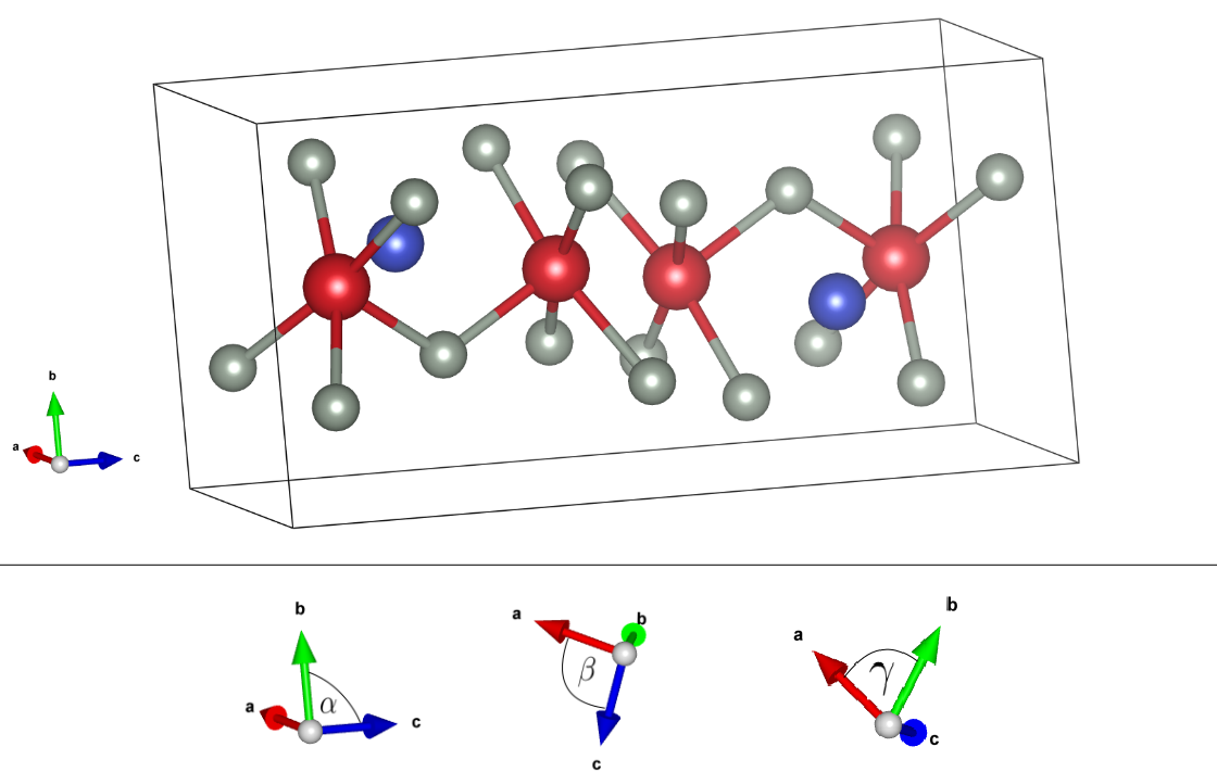
Figure 1: Orthorhombic unit cell. The Tantalum atoms are depicted in red, the Nickel atoms in blue and the Selenium atoms in grey. In the lower part the three angles of the cell are displayed

III Minimal model

We consider a two-dimensional minimal model with six atoms per unit cell (with one $d_{xz}$-like orbital each) reproducing the double chain structure of a Ta₂NiSe₅ layer. We take into account $i)$ single particle hoppings, $ii)$ intra-atomic density-density interactions, and $iii)$ nearest-neighbor density-density interactions. For simplicity we recall here the definition of the Hamiltonian which we already introduced in the main text:

$$\begin{split}\hat{\cal H}=&\hat{H}_{hop}+\hat{H}_{U}+\hat{H}_{V}\\ =&\sum_{\vec{R}\sigma}\sum_{\vec{\delta}}\Psi^{\dagger}_{\vec{R}+\vec{\delta}}\mathbf{T}(\vec{\delta})\Psi_{\vec{R}\sigma}+U\sum_{\vec{R}}\sum_{j=1,\ldots,6}\hat{n}_{j\uparrow}(\vec{R})\hat{n}_{j\downarrow}(\vec{R})+\\ &+V\sum_{j=1,2}\sum_{\vec{R}\sigma\sigma^{\prime}}\left[\hat{n}_{j\sigma}(\vec{R})+\hat{n}_{j\sigma}(\vec{R}+\vec{\delta}_{x})\right]\hat{n}_{5\sigma^{\prime}}(\vec{R})+V\sum_{j=3,4}\sum_{\vec{R}\sigma\sigma^{\prime}}\left[\hat{n}_{j\sigma}(\vec{R})+\hat{n}_{j\sigma}(\vec{R}-\vec{\delta}_{x})\right]\hat{n}_{6\sigma^{\prime}}(\vec{R}),\end{split}$$ (1)

with $\Psi_{\vec{R}\sigma}$ a spinor defined as $\Psi_{\vec{R}\sigma}^{\dagger}\equiv\left(c^{\dagger}_{1\sigma}(\vec{R})\leavevmode\nobreak\ c^{\dagger}_{2\sigma}(\vec{R})\leavevmode\nobreak\ c^{\dagger}_{5\sigma}(\vec{R})\leavevmode\nobreak\ c^{\dagger}_{3\sigma}(\vec{R})\leavevmode\nobreak\ c^{\dagger}_{4\sigma}(\vec{R})\leavevmode\nobreak\ c^{\dagger}_{6\sigma}(\vec{R})\right)$ and $\hat{n}_{i\sigma}(\vec{R})=c^{\dagger}_{i\sigma}(\vec{R})c^{\phantom{\dagger}}_{i\sigma}(\vec{R})$. The hopping matrix $\mathbf{T}(\vec{\delta})$ contains intra-cell [$\mathbf{T}(\vec{0})$] as well as nearest-cells terms [$\mathbf{T}(\pm a_{x},\pm a_{y})$] corresponding to the main contributions of the Wannier Hamiltonian derived above. These matrix elements are summarized in the scheme of Fig. 2(A), which includes Ta-Ta (a) and Ni-Ni (b) intra-chain, Ta-Ni intra- (c)-(d) and inter-chain (e)-(f) hoppings as well as inter-chain Ni-Ni (g) and Ta-Ta (j)-(h) hoppings. Dashed/full pairs of arrows indicate that in order to preserve the symmetry, these matrix elements must be anti-symmetric under a reflection with respect to a plane perpendicular to the chains. We have also indicated symmetry-forbidden Ta-Ni hybridization, that become non-zero upon symmetry breaking. The matrix elements are summarized in the Table 1. Fig. 2(B) shows the comparison between the band structure of the minimal and the Wannier model.

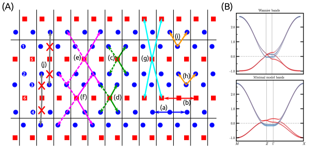
Figure 2: (A) Hopping processes defining the minimal model. Letters are used to group different hopping processes according to the table 1. (B) Comparison between the Wannier (top) and the minimal model (bottom) band structure.

Hopping matrix elements $\mathbf{T}(\vec{\delta})$
Intra-chain Ta-Ta hopping (a)-(b)	$T_{ii}(a_{x},0)=T_{ii}(-a_{x},0)=-0.72\leavevmode\nobreak\ \mathrm{eV}\quad i=1,\ldots,4$
	$T_{ii}(0,0)=1.35\leavevmode\nobreak\ \mathrm{eV}$
Intra-chain Ni-Ni hopping (a)-(b)	$T_{ii}(a_{x},0)=T_{ii}(-a_{x},0)=0.30\leavevmode\nobreak\ \mathrm{eV}\quad i=5,6$
	$T_{ii}(0,0)=-0.36\leavevmode\nobreak\ \mathrm{eV}$
Intra-chain Ta-Ni hopping (c)-(d)	$T_{15}(\vec{0})=-T_{15}(a_{x},0)=T_{25}(\vec{0})=-T_{25}(a_{x},0)=0.035\leavevmode\nobreak\ \mathrm{eV}$
	$T_{36}(\vec{0})=T_{46}(\vec{0})=-T_{15}(\vec{0})$
Inter-chain Ta-Ni hopping (e)-(f)	$T_{45}(-a_{x},a_{y})=-T_{45}(a_{x},a_{y})=T_{35}(a_{x},0)=-T_{35}(-a_{x},0)=0.04\leavevmode\nobreak\ \mathrm{eV}$
	$T_{26}(a_{x},0)=T_{16}(a_{x},-a_{y})=T_{45}(a_{x},a_{y})$
Inter-chain Ni-Ni hopping (g)	$T_{65}(a_{x},a_{y})=T_{65}(a_{x},0)=T_{65}(0,0)=T_{65}(a_{x},0)=0.030\leavevmode\nobreak\ \mathrm{eV}$
Inter-chain Ta-Ta hopping (h)-(i)	$T_{61}(-a_{x},a_{y})=T_{61}(0,a_{y})=T_{23}(0,0)=T_{23}(a_{x},0)=0.020\leavevmode\nobreak\ \mathrm{eV}$

Table 1: Elements of the hopping matrix $\mathbf{T}(\vec{\delta})$. Matrix elements are grouped accordingly to the scheme in Fig. 2 with letters corresponding to the different hopping processes indicated by arrows.

III.1 Hartree-Fock

We consider a single-particle variational wavefunction $|{\Psi_{0}}\rangle$ that allows for the breaking of the crystal symmetries. The variational energy is computed by decoupling the interaction terms in the standard way:

$$\langle{\Psi_{0}}|{\hat{n}_{j\uparrow}(\vec{R})\hat{n}_{j\downarrow}(\vec{R})}|{\Psi_{0}}\rangle\approx\langle{\Psi_{0}}|{\hat{n}_{j\uparrow}(\vec{R})}|{\Psi_{0}}\rangle\langle{\Psi_{0}}|{\hat{n}_{j\downarrow}(\vec{R})}|{\Psi_{0}}\rangle$$ (2)

and for $i\neq j$

$$\langle{\Psi_{0}}|{\hat{n}_{j\sigma}(\vec{R})\hat{n}_{i\sigma^{\prime}}(\vec{R^{\prime}})}|{\Psi_{0}}\rangle\approx\langle{\Psi_{0}}|{\hat{n}_{j\sigma}(\vec{R})}|{\Psi_{0}}\rangle\langle{\Psi_{0}}|{\hat{n}_{i\sigma^{\prime}}(\vec{R^{\prime}})}|{\Psi_{0}}\rangle-\delta_{\sigma\sigma^{\prime}}\langle{\Psi_{0}}|{c^{\dagger}_{j\sigma}(\vec{R})c^{\phantom{\dagger}}_{i\sigma^{\prime}}(\vec{R^{\prime}})}|{\Psi_{0}}\rangle\langle{\Psi_{0}}|{c^{\dagger}_{i\sigma^{\prime}}(\vec{R^{\prime}})c^{\phantom{\dagger}}_{j\sigma}(\vec{R})}|{\Psi_{0}}\rangle.$$ (3)

Taking the variation with respect to $\left\langle{\Psi_{0}}\right|$ the HF Hamiltonian reads

$$\hat{H}_{HF}=\hat{H}_{hop}+\sum_{{\bf k}\sigma}\Psi^{\dagger}_{{\bf k}\sigma}\left(\begin{matrix}\hat{h}_{A}({\bf k})&0\\ 0&\hat{h}_{B}({\bf k})\end{matrix}\right)\Psi_{{\bf k}\sigma}$$ (4)

where $\hat{h}_{A}({\bf k})$ and $\hat{h}_{B}({\bf k})$ are the decoupled interaction Hamiltonian for the A and B chain respectively. Specifically, accordingly to the atom labeling of Fig. 2,

$$\hat{h}_{A}({\bf k})=\left(\begin{matrix}\delta\varepsilon_{1}&0&w_{15}^{*}({\bf k})\\ 0&\delta\varepsilon_{2}&w^{*}_{25}({\bf k})\\ w_{15}({\bf k})&w_{25}({\bf k})&\delta\varepsilon_{5}\end{matrix}\right)\qquad\hat{h}_{B}({\bf k})=\left(\begin{matrix}\delta\varepsilon_{3}&0&w_{36}^{*}({\bf k})\\ 0&\delta\varepsilon_{4}&w^{*}_{46}({\bf k})\\ w_{46}({\bf k})&w_{46}({\bf k})&\delta\varepsilon_{6}\end{matrix}\right)$$ (5)

with

$$\delta\varepsilon_{i=1,2}=\frac{U}{2}n_{i}+2Vn_{5}\quad\delta\varepsilon_{i=3,4}=\frac{U}{2}n_{i}+2Vn_{6}\quad\delta\varepsilon_{5}=\frac{U}{2}n_{5}+2V\left(n_{1}+n_{2}\right)\quad\delta\varepsilon_{6}=\frac{U}{2}n_{6}+2V\left(n_{3}+n_{4}\right)$$ (6)

and

$$w_{i5}=-V\Delta_{i5}(\vec{0})(1-e^{-ik_{x}a})-V\phi_{i5}e^{-ik_{x}a}\quad w_{i6}=-V\Delta_{i6}(\vec{0})(1-e^{ik_{x}a})-V\phi_{i6}e^{ik_{x}a}.$$ (7)

In these equations $n_{i}=\langle{\Psi_{0}}|{c^{\dagger}_{i\sigma}(\vec{0})c^{\phantom{\dagger}}_{i\sigma}(\vec{0})}|{\Psi_{0}}\rangle$, $\Delta_{ij}(\vec{0})=\langle{\Psi_{0}}|{c^{\dagger}_{i\sigma}(\vec{0})c^{\phantom{\dagger}}_{j\sigma}(\vec{0})}|{\Psi_{0}}\rangle$ and $\phi_{ij}$ are the order parameters defined in the main text. All the above parameters are self-consistently determined by diagonalizing the HF Hamiltonian starting from an initial guess.

III.2 Double Counting Corrections

To avoid double counting of correlation effects within our Hartree-Fock calculations which are already present on the level of the DFT calculations, we make use of cRPA Coulomb matrix elements and apply a double counting correction potential to the bare band structure. The former aims to avoid a double counting of screening processes to the Coulomb interactions resulting from the model band structure. By excluding these screening processes in cRPA calculations for the Coulomb matrix elements based on the full ab initio band structure we take screening from the ”rest” of the band structure into account, but not from the bands of the minimal model. A double counting of this kind is thus avoided in the interaction terms. On the other side, the double-counting potential is introduced to not count twice the effect of local interactions already included in DFT. The commonly used ansatz for this is an orbital-independent potential which is acting only on the correlated orbitals. Since our minimal model is completely down-folded to correlated orbitals only, a potential of this form would equally shift all involved bands and would thus have no effect at all. We can thus safely neglect a double-counting correction potential of this form.

Care must, however, be taken due to the use of the modified Becke-Johnson (mbj) exchange potential (in contrast to GGA or LDA approximations). Although this exchange potential is still local, it effectively accounts for non-local Coulomb interaction terms here. The most prominent effect of the mbj exchange potential for Ta₂NiSe₅ is to decrease the overlap between the mostly Ta-like conduction bands with the mostly Ni-like valence bands, which is controlled by the mbj parameter $c_{\text{mbj}}$. For $c_{\text{mbj}}=1.0$ the results are very similar to GGA/LDA calculations with a an overlap of about $400\,$meV at $Z$. For our self-consistently calculated $c_{\text{mbj}}=1.26$ the overlap is approx. $200\,$meV. In order to not double-count this decreasing trend of the overlap upon inclusion of correlation effects, the Ta and Ni onsite energies of our minimal model are adjusted to result in an overlap of about $400\,$meV (see Fig. 2 B). We also checked the influence of this procedure and find that all of our conclusions hold independently on the exact value of this change in the overlap. The phase diagram looks qualitatively the same and just slight quantitative changes are observed so that the critical values $V_{l}^{*}(U)$ and $V_{u}^{*}(U)$ shift to slightly larger values upon increasing the band overlap in the bare minimal model.