Transverse-Legendrian links

Abstract.

In recent joint works of the present author with M. Prasolov and V. Shastin a new technique for distinguishing Legendrian knots has been developed. In this paper the technique is extended further to provide a tool for distinguishing transverse knots. It is shown that the equivalence problem for transverse knots with trivial orientation-preserving symmetry group is algorithmically solvable. In a future paper the triviality condition for the orientation-preserving symmetry group will be dropped.

1. Introduction

Rectangular (or grid) diagrams of links provide a convenient combinatorial framework for studying Legendrian and transverse links. Namely, there are the following naturally defined bijections, each respecting the topological type of the link:

$$\mathscr{R}/\bigl{\langle}\overrightarrow{\mathrm{I}},\overleftarrow{\mathrm{I}}\bigr{\rangle} \cong\bigl{\{}\xi_{+}\text{-Legendrian link types}\big{\}},$$

$$\mathscr{R}/\bigl{\langle}\overrightarrow{\mathrm{II}},\overleftarrow{\mathrm{II}}\bigr{\rangle} \cong\bigl{\{}\xi_{-}\text{-Legendrian link types}\big{\}},$$

$$\mathscr{R}/\bigl{\langle}\overrightarrow{\mathrm{I}},\overleftarrow{\mathrm{I}},\overleftarrow{\mathrm{II}}\bigr{\rangle}\cong\mathscr{R}/\bigl{\langle}\overrightarrow{\mathrm{I}},\overleftarrow{\mathrm{I}},\overrightarrow{\mathrm{II}}\bigr{\rangle} \cong\bigl{\{}\xi_{+}\text{-transverse link types}\big{\}},$$

$$\mathscr{R}/\bigl{\langle}\overrightarrow{\mathrm{I}},\overleftarrow{\mathrm{II}},\overrightarrow{\mathrm{II}}\bigr{\rangle}\cong\mathscr{R}/\bigl{\langle}\overleftarrow{\mathrm{I}},\overleftarrow{\mathrm{II}},\overrightarrow{\mathrm{II}}\bigr{\rangle} \cong\bigl{\{}\xi_{-}\text{-transverse link types}\big{\}},$$

where $\mathscr{R}/\langle T_{1},\ldots,T_{k}\rangle$ means ‘oriented rectangular diagrams viewed up to exchange moves and (de)stabilizations of oriented types $T_{1},\ldots,T_{k}$’ (we use the notation of [5] for the oriented types of stabilizations and destabilizations; see also Definition 3.2 and Figure 3 below), $\xi_{+}$ is the standard contact structure of $\mathbb{S}^{3}$, and $\xi_{-}$ is the mirror image of $\xi_{+}$. A proof of these facts can be found in [10].

With the notation above at hand, the elements of the sets

$$\mathscr{R}/\bigl{\langle}\overrightarrow{\mathrm{I}},\overrightarrow{\mathrm{II}}\bigr{\rangle}\cong\mathscr{R}/\bigl{\langle}\overleftarrow{\mathrm{I}},\overleftarrow{\mathrm{II}}\bigr{\rangle}\cong\mathscr{R}/\bigl{\langle}\overrightarrow{\mathrm{I}},\overleftarrow{\mathrm{II}}\bigr{\rangle}\cong\mathscr{R}/\bigl{\langle}\overleftarrow{\mathrm{I}},\overrightarrow{\mathrm{II}}\bigr{\rangle}$$

are naturally interpreted as braids viewed up to conjugacy and Birman–Menasco exchange moves defined in [1] (these entities are called Birman–Menasco classes in [5]), and elements of

$$\mathscr{R}/\bigl{\langle}\overrightarrow{\mathrm{I}},\overleftarrow{\mathrm{I}},\overrightarrow{\mathrm{II}},\overleftarrow{\mathrm{II}}\bigr{\rangle}$$

as topological types of oriented links in $\mathbb{S}^{3}$, see [3, 4].

The elements of $\mathscr{R}/\langle\varnothing\rangle$ are so called exchange classes, which mean rectangular diagrams viewed up to exchange moves. The number of possible combinatorial types of diagrams in each exchange class is finite, so the equivalence problem for exchange classes is trivially decidable. This fact and the results of [6] are used in [7] to solve the equivalence problem for Legendrian knots of topological types having trivial orientation-preserving symmetry group. It is noted in [7] that the equivalence problem for transverse knots of the same topological types can be solved in a similar manner, once we are able to solve the equivalence problem for the elements of $\mathscr{R}/\bigl{\langle}\overrightarrow{\mathrm{I}}\bigr{\rangle}$, $\mathscr{R}/\bigl{\langle}\overleftarrow{\mathrm{I}}\bigr{\rangle}$, $\mathscr{R}/\bigl{\langle}\overrightarrow{\mathrm{II}}\bigr{\rangle}$, and $\mathscr{R}/\bigl{\langle}\overleftarrow{\mathrm{II}}\bigr{\rangle}$ (see [7, Remark 7.1]).

In this note we give a topological interpretation to the elements of these sets and solve the equivalence problem for them, thus extending the method of [6, 7] to transverse knots.

2. Notation

We denote by $\mathbb{T}^{2}$ the two-dimensional torus $\mathbb{S}^{1}\times\mathbb{S}^{1}$, and by $\theta,\varphi$ the angular coordinates on $\mathbb{T}^{2}$, which run through $\mathbb{R}/(2\pi\mathbb{Z})$. Denote by $p_{\theta}$ and $p_{\varphi}$ the projection maps from $\mathbb{T}^{2}$ to the first and the second $\mathbb{S}^{1}$-factors, respectively.

We regard the three-sphere $\mathbb{S}^{3}$ as the join $\mathbb{S}^{1}*\mathbb{S}^{1}$ of two circles, and use the associated coordinate system $\theta,\varphi,\tau$:

$$\mathbb{S}^{3}=\mathbb{S}^{1}\times\mathbb{S}^{1}\times[0;1]/\bigl{(}(\theta^{\prime},\varphi,0)\sim(\theta^{\prime\prime},\varphi,0),(\theta,\varphi^{\prime},1)\sim(\theta,\varphi^{\prime\prime},1)\ \forall\theta,\theta^{\prime},\theta^{\prime\prime},\varphi,\varphi^{\prime},\varphi^{\prime\prime}\in\mathbb{S}^{1}\bigr{)}.$$

(Observe that $\tau$ is set to $1$ on the first copy of $\mathbb{S}^{1}$, on which the angular coordinate is $\theta$, and to $0$ on the second one, where the angular coordinate is $\varphi$.)

The map $p_{\theta,\varphi}:\mathbb{S}^{3}\setminus\bigl{(}\mathbb{S}^{1}_{\tau=1}\cup\mathbb{S}^{1}_{\tau=0}\bigr{)}\rightarrow\mathbb{T}^{2}$ defined by $p_{\theta,\varphi}(\theta,\varphi,\tau)=(\theta,\varphi)$ is referred to as the torus projection.

For two distinct points $x_{1},x_{2}\in\mathbb{S}^{1}$ we denote by $[x_{1};x_{2}]$ (respectively, $(x_{1};x_{2})$) the closed (respectively, open) interval in $\mathbb{S}^{1}$ starting at $x_{1}$ and ending at $x_{2}$.

3. Rectangular diagrams of links

Definition 3.1.

By an oriented rectangular diagram of a link we mean a non-empty finite subset $R\subset\mathbb{T}^{2}$ with a decomposition $R=R^{+}\sqcup R^{-}$ into disjoint union of two subsets $R^{+}$ and $R^{-}$ such that we have $p_{\theta}(R^{+})=p_{\theta}(R^{-})$, $p_{\varphi}(R^{+})=p_{\varphi}(R^{-})$, and each of $p_{\theta}$, $p_{\varphi}$ restricted to each of $R^{+}$, $R^{-}$ is injective.

The elements of $R$ (respectively, of $R^{+}$ or $R^{-}$) are called vertices (respectively, positive vertices or negative vertices) of $R$.

Pairs $(u,v)$ of vertices of $R$ such that $p_{\theta}(u)=p_{\theta}(v)$ (respectively, $p_{\varphi}(u)=p_{\varphi}(v)$) are called vertical (respectively, horizontal) edges of $R$.

With every oriented rectangular diagram $R$ of a link we define the associated oriented link $\widehat{R}\subset\mathbb{S}^{3}$ as the closure of the preimage $p_{\theta,\varphi}^{-1}(R)$ oriented so that $\tau$ increases on the oriented arcs constituting $p_{\theta,\varphi}^{-1}(R^{+})$ and decreases on the oriented arcs constituting $p_{\theta,\varphi}^{-1}(R^{-})$.

A planar diagram of a link topologically equivalent to $\widehat{R}$ can be obtained as follows. Cut the torus $\mathbb{T}^{2}$ along a longitude and a meridian not passing through a vertex of $R$ to obtain a square. Connect the vertices in every edge by a vertical or horizontal straight line segment and make all verticals overpasses at all crossings. Orient the obtained diagram so that each vertical edge is directed from a positive vertex to a negative one, and each horizontal edge from a negative to a positive one. For an example see Figure 1, where positive vertices are black and negative ones are white.

$R$		a knot equivalent to $\widehat{R}$

Figure 1. A rectangular diagram of a link and a planar diagram of the corresponding link

In this paper, all links and their diagrams are assumed to be oriented, so we omit ‘oriented’ in the sequel.

Definition 3.2.

Let $R_{1}$ and $R_{2}$ be rectangular diagrams of a link such that, for some $\theta_{1},\theta_{2},\varphi_{1},\varphi_{2}\in\mathbb{S}^{1}$, the following holds:

1. $\theta_{1}\neq\theta_{2}$, $\varphi_{1}\neq\varphi_{2}$;

2. the symmetric difference $R_{1}\triangle R_{2}$ is $\{\theta_{1},\theta_{2}\}\times\{\varphi_{1},\varphi_{2}\}$;

3. the intersection of the rectangle $[\theta_{1};\theta_{2}]\times[\varphi_{1};\varphi_{2}]$ with $R_{1}\cup R_{2}$ coincides with $R_{1}\triangle R_{2}$;

4. one, two, or three consecutive corners of the rectangle $[\theta_{1};\theta_{2}]\times[\varphi_{1};\varphi_{2}]$ belong to $R_{1}$, and the other(s) to $R_{2}$;

5. the orientations of $R_{1}$ and $R_{2}$ agree on $R_{1}\cap R_{2}$, which means $R_{1}^{+}\cap R_{2}=R_{1}\cap R_{2}^{+}$ (equivalently, $R_{1}^{-}\cap R_{2}=R_{1}\cap R_{2}^{-}$).

Then we say that the passage $R_{1}\mapsto R_{2}$ is an elementary move.

An elementary move $R_{1}\mapsto R_{2}$ is called:

• an exchange move if $|R_{1}|=|R_{2}|$,

• a stabilization move if $|R_{2}|=|R_{1}|+2$, and

• a destabilization move if $|R_{2}|=|R_{1}|-2$,

where $|R|$ denotes the number of vertices of $R$.

We distinguish two types and four oriented types of stabilizations and destabilizations as follows.

Definition 3.3.

Let $R_{1}\mapsto R_{2}$ be a stabilization, and let $\theta_{1},\theta_{2},\varphi_{1},\varphi_{2}$ be as in Definition 3.2. Denote by $v$ an element of $R_{1}\cap([\theta_{1};\theta_{2}]\times[\varphi_{1};\varphi_{2}])$, which is unique. We say that the stabilization $R_{1}\mapsto R_{2}$ and the destabilization $R_{2}\mapsto R_{1}$ are of type I (respectively, of type II) if $v\in\{(\theta_{1},\varphi_{1}),(\theta_{2},\varphi_{2})\}$ (respectively, $v\in\{(\theta_{1},\varphi_{2}),(\theta_{2},\varphi_{1})\}$).

Let $\varphi_{0}\in\{\varphi_{1},\varphi_{2}\}$ be such that $\{\theta_{1},\theta_{2}\}\times\{\varphi_{0}\}\subset R_{2}$. The stabilization $R_{1}\mapsto R_{2}$ and the destabilization $R_{2}\mapsto R_{1}$ are of oriented type $\overrightarrow{\mathrm{I}}$ (respectively, of oriented type $\overrightarrow{\mathrm{II}}$) if they are of type I (respectively, of type II), and $(\theta_{2},\varphi_{0})$ is a positive vertex of $R_{2}$. The stabilization $R_{1}\mapsto R_{2}$ and the destabilization $R_{2}\mapsto R_{1}$ are of oriented type $\overleftarrow{\mathrm{I}}$ (respectively, of oriented type $\overleftarrow{\mathrm{II}}$) if they are of type I (respectively, of type II) and $(\theta_{2},\varphi_{0})$ is a negative vertex of $R_{2}$.

Elementary moves are illustrated in Figures 2 and 3, where the shaded rectangle is supposed to contain no vertices of the diagrams except the indicated ones.

	$\leftrightarrow$				$\leftrightarrow$
	$\leftrightarrow$				$\leftrightarrow$

Figure 2. Exchange moves

	$\leftrightarrow$				$\leftrightarrow$
	type $\overrightarrow{\mathrm{I}}$				type $\overrightarrow{\mathrm{I}}$
	$\leftrightarrow$				$\leftrightarrow$
	type $\overleftarrow{\mathrm{I}}$				type $\overleftarrow{\mathrm{I}}$
	$\leftrightarrow$				$\leftrightarrow$
	type $\overrightarrow{\mathrm{II}}$				type $\overrightarrow{\mathrm{II}}$
	$\leftrightarrow$				$\leftrightarrow$
	type $\overleftarrow{\mathrm{II}}$				type $\overleftarrow{\mathrm{II}}$

Figure 3. Stabilization and destabilization moves

The set of all rectangular diagrams of links will be denoted by $\mathscr{R}$. For any subset $\{T_{1},\ldots,T_{k}\}$ of $\{\overrightarrow{\mathrm{I}},\overleftarrow{\mathrm{I}},\overrightarrow{\mathrm{II}},\overleftarrow{\mathrm{II}}\}$, we denote by $\langle T_{1},\ldots,T_{k}\rangle$ the equivalence relation on $\mathscr{R}$ generated by all stabilizations and destabilizations of oriented types $T_{1},\ldots,T_{k}$ and exchange moves. For a rectangular diagram of a link $R\in\mathscr{R}$, we denote by $[R]_{T_{1},\ldots,T_{k}}$ the equivalence class of $R$ in $\mathscr{R}/\langle T_{1},\ldots,T_{k}\rangle$.

The following statement is nearly a reformulation of [3, Proposition on page 42 + Theorem on page 45] and [4, Proposition 4] (the three versions use slightly different settings and sets of moves, but their equivalence is easily seen).

Theorem 3.1.

The map

$$R\mapsto\text{the topological type of }\widehat{R}$$

establishes a one-to-one correspondence between $\mathscr{R}/\langle\overrightarrow{\mathrm{I}},\overleftarrow{\mathrm{I}},\overrightarrow{\mathrm{II}},\overleftarrow{\mathrm{II}}\rangle$ and the set of all link types.

4. Decidability for the equivalence of transverse knots

Here is the main technical result of the present paper:

Theorem 4.1.

For any $T\in\{\overrightarrow{\mathrm{I}},\overleftarrow{\mathrm{I}},\overrightarrow{\mathrm{II}},\overleftarrow{\mathrm{II}}\}$ there is an algorithm for deciding, given two rectangular diagrams of a link $R_{1}$, $R_{2}$, whether or not $[R_{1}]_{T}=[R_{2}]_{T}$.

To prove Theorem 4.1 we need some preparations.

For a rectangular diagram of a link $R$, denote by $\Gamma_{\overrightarrow{\mathrm{II}}}(R)$ the following union of closed immersed staircase-like curves in $\mathbb{T}^{2}$:

$$\Gamma_{\overrightarrow{\mathrm{II}}}(R)=\left(\bigcup_{(\theta_{0},\varphi_{1})\in R^{+},\ (\theta_{0},\varphi_{2})\in R^{-}}\{\theta_{0}\}\times[\varphi_{1};\varphi_{2}]\right)\cup\left(\bigcup_{(\theta_{1},\varphi_{0})\in R^{-},\ (\theta_{2},\varphi_{0})\in R^{+}}[\theta_{1};\theta_{2}]\times\{\varphi_{0}\}\right)$$

oriented by demanding that $\theta+\varphi$ locally increase on every straight line segment in this union. These straight line segments will be referred to as the edges of $\Gamma_{\overrightarrow{\mathrm{II}}}(R)$. Thus, the pair of endpoints of an edge of $\Gamma_{\overrightarrow{\mathrm{II}}}(R)$ is an edge of $R$, and vice versa.

An example is shown in Figure 4.

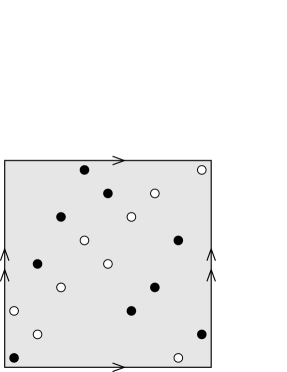
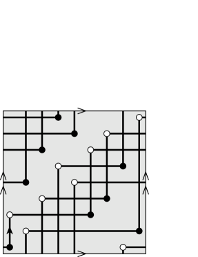
$R$		$\Gamma_{\overrightarrow{\mathrm{II}}}(R)$

Figure 4. A rectangular diagram of a link $R$ and the curve $\Gamma_{\overrightarrow{\mathrm{II}}}(R)$

The union of curves $\Gamma_{\overrightarrow{\mathrm{II}}}(R)$ can also be described as the torus projection of the link $\widehat{R}_{\varepsilon}$ obtained from $\widehat{R}$ by replacing each arc in the domain $\tau\in[0;\varepsilon]$ (respectively, $\tau\in[1-\varepsilon;1]$) by an arc on which the coordinates $\varphi$ and $\tau$ are constant, and $\theta$ is increasing (respectively, $\theta$ and $\tau$ are constant, and $\varphi$ is increasing), where $\varepsilon\in(0;1/2)$.

With every rectangular diagram of a link $R$ we associate a triple of numbers $\omega_{\overrightarrow{\mathrm{II}}}(R)\in\mathbb{N}\times\mathbb{N}\times(\mathbb{N}\cup\{0\})$ as follows: $\omega_{\overrightarrow{\mathrm{II}}}(R)=(k,l,m)$, where $m$ is the number of double points in $\Gamma_{\overrightarrow{\mathrm{II}}}(R)$, and $(k,l)\in\mathbb{Z}^{2}=H_{1}(\mathbb{T}^{2};\mathbb{Z})$ is the homology class of $\Gamma_{\overrightarrow{\mathrm{II}}}(R)$, that is,

$$k=\frac{1}{2\pi}\int\limits_{\Gamma_{\overrightarrow{\mathrm{II}}}(R)}d\theta,\qquad l=\frac{1}{2\pi}\int\limits_{\Gamma_{\overrightarrow{\mathrm{II}}}(R)}d\varphi.$$

Lemma 4.1.

If $[R]_{\overrightarrow{\mathrm{II}}}=[R^{\prime}]_{\overrightarrow{\mathrm{II}}}$, then $\omega_{\overrightarrow{\mathrm{II}}}(R)=\omega_{\overrightarrow{\mathrm{II}}}(R^{\prime})$.

Proof.

To simplify the notation we put $\Gamma=\Gamma_{\overrightarrow{\mathrm{II}}}(R)$ and $\Gamma^{\prime}=\Gamma_{\overrightarrow{\mathrm{II}}}(R^{\prime})$. It suffices to consider the case when $R\mapsto R^{\prime}$ is an exchange move or a type $\overrightarrow{\mathrm{II}}$ stabilization. One can check that, for any of these moves, the closure of the symmetric difference $\Gamma\triangle\Gamma^{\prime}$ is the boundary of a rectangle $r$ (which is not necessarily the one mentioned in Definition 3.2), with the bottom and right sides of $r$ belonging to one of $\Gamma$, $\Gamma^{\prime}$, and the top and left sides to the other. Moreover, if $\Gamma$ and $\Gamma^{\prime}$ are viewed as $1$-chains, then $\Gamma-\Gamma^{\prime}=\partial r$ for some orientation of $r$. The cases are sketched in Figure 5.

	$\leftrightarrow$				$\leftrightarrow$
	$\leftrightarrow$				$\leftrightarrow$

Figure 5. The change of $\Gamma_{\overrightarrow{\mathrm{II}}}(R)$ under allowed elementary moves on $R$

Thus, the homology class of $\Gamma$ in $H_{1}(\mathbb{T}^{2})$ is the same as that of $\Gamma^{\prime}$. Let $(k,l)\in H_{1}(\mathbb{T}^{2};\mathbb{Z})$ be this class.

Since both multi-valued functions $\theta$ and $\varphi$ are locally non-decreasing on every edge of $\Gamma$ and $\Gamma^{\prime}$, each meridian $\{\theta\}\times\mathbb{S}^{1}$ (respectively, longitude $\mathbb{S}^{1}\times\{\varphi\}$) not passing through a vertex of $R$ intersects each of $\Gamma$ and $\Gamma^{\prime}$ exactly $k$ (respectively, $l$) times.

Let $\theta_{1},\theta_{2},\varphi_{1},\varphi_{2}$ be as in Definition 3.2. Denote the rectangle $[\theta_{1};\theta_{2}]\times[\varphi_{1};\varphi_{2}]$ by $r_{0}$. Three cases are possible:

• $r=r_{0}$,

• $r=[\theta_{2};\theta_{1}]\times[\varphi_{1};\varphi_{2}]$, or

• $r=[\theta_{1};\theta_{2}]\times[\varphi_{2};\varphi_{1}]$.

By the assumption of Definition 3.2, the intersection of $r_{0}$ with $R$ is a subset of the set of vertices of $r_{0}$. Therefore, any vertical edge of $\Gamma$ that intersects $(\theta_{1};\theta_{2})\times\{\varphi_{1}\}$ intersects also $(\theta_{1};\theta_{2})\times\{\varphi_{2}\}$, and vice versa. Let $k_{0}$ be the number of such edges. These edges are the same in $\Gamma^{\prime}$.

Similarly, let $l_{0}$ be the number of horizontal edges of $\Gamma$ (equivalently, of $\Gamma^{\prime}$) that intersect $\{\theta_{1}\}\times(\varphi_{1};\varphi_{2})$ (equivalently, $\{\theta_{2}\}\times(\varphi_{1};\varphi_{2})$).

$\Gamma$ and $\Gamma^{\prime}$ have exactly the same set of double points outside $\partial r$. From the arguments above it follows that the number of double points of $\Gamma$ and $\Gamma^{\prime}$ at $\partial r$ is also the same and is equal to

• $k_{0}+l_{0}$ if $r=r_{0}$,

• $k-k_{0}-1+l_{0}$ if $r=[\theta_{2};\theta_{1}]\times[\varphi_{1};\varphi_{2}]$,

• $k_{0}+l-l_{0}-1$ if $r=[\theta_{1};\theta_{2}]\times[\varphi_{2};\varphi_{1}]$.

The claim follows. ∎

Lemma 4.2.

Let $R$ and $R^{\prime}$ be rectangular diagrams of a link such that the closure of the symmetric difference $\Gamma_{\overrightarrow{\mathrm{II}}}(R)\triangle\Gamma_{\overrightarrow{\mathrm{II}}}(R^{\prime})$ has the form of the boundary of an embedded disk or an annulus $F\subset\mathbb{T}^{2}$ such that the interior of $F$ is disjoint from $R\cup R^{\prime}$, and $\partial F$ is disjoint from the set of double points of $\Gamma_{\overrightarrow{\mathrm{II}}}(R)$ and $\Gamma_{\overrightarrow{\mathrm{II}}}(R^{\prime})$. Then $[R]_{\overrightarrow{\mathrm{II}}}=[R^{\prime}]_{\overrightarrow{\mathrm{II}}}$.

Proof.

We again put $\Gamma=\Gamma_{\overrightarrow{\mathrm{II}}}(R)$ and $\Gamma^{\prime}=\Gamma_{\overrightarrow{\mathrm{II}}}(R^{\prime})$. Suppose that $F$ is a disc. It follows from the hypothesis of the lemma that:

1. $F$ is co-bounded by two staircase arcs $\alpha$ and $\beta$ such that $\alpha\subset\Gamma$ and $\beta\subset\Gamma^{\prime}$ (on which the functions $\theta$ and $\varphi$ are locally non-decreasing);

2. the set of corners of $F$ coincides with $R\triangle R^{\prime}$.

See Figure 6(a) for an illustration.

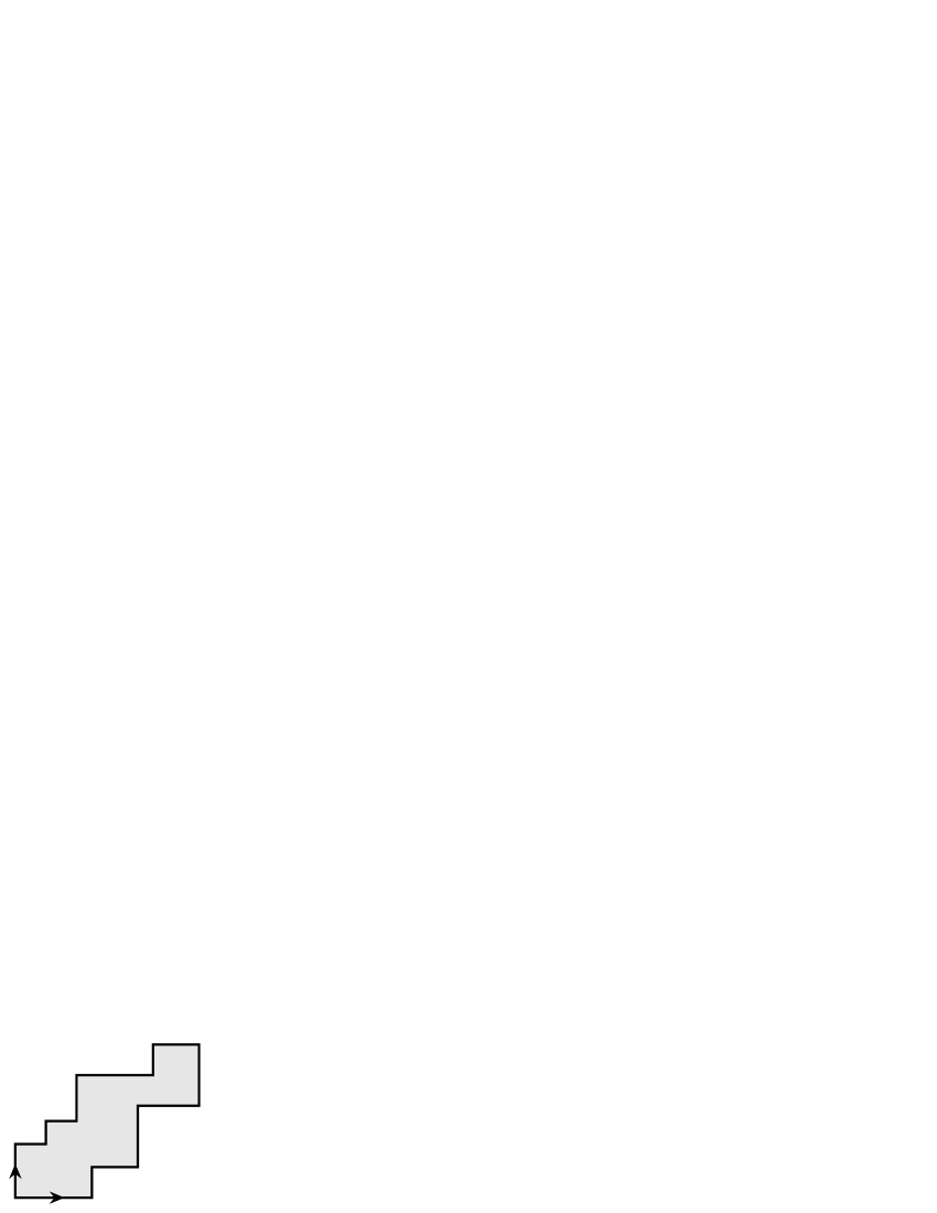
(a)		(b)

Figure 6. Induction step when $F$ is a disc

The proof is by induction in the number $m$ of corners of the polygon $F$. The smallest possible number is $m=4$. In this case, one easily finds that $R\mapsto R^{\prime}$ is an exchange move or a type $\overrightarrow{\mathrm{II}}$ stabilization or destabilization.

Suppose that $m>4$ and the claim is proved in the case when $F$ has fewer corners than $m$. Small perturbations of a rectangular diagram of a link are achievable by means exchange moves, so, without loss of generality, we may assume that no meridian or longitude of the torus $\mathbb{T}^{2}$ contains four points of $R\cup R^{\prime}$, for this can be resolved by a small perturbation of $R$ or $R^{\prime}$.

There is an arc $\gamma$ of the form $[\theta_{1};\theta_{2}]\times\{\varphi_{0}\}$ such that:

1. $\gamma\subset F$;

2. $\gamma\cap\partial F=\partial\gamma$;

3. one of the endpoints of $\gamma$ belongs to $R\cup R^{\prime}$.

Without loss of generality we may assume that $(\theta_{1},\varphi_{0})\in\alpha$ and $(\theta_{2},\varphi_{0})\in\beta$ as this is the question of exchanging the roles of $R$ and $R^{\prime}$. The arc $\gamma$ cuts $F$ into two discs, which we denote by $F_{1}$ and $F_{2}$. We number them so that $F_{1}$ is above $\gamma$ and $F_{2}$ is below $\gamma$, see Figure 6(b).

Let $C_{1}$ (respectively, $C_{2}$) be the set of corners of $F_{1}$ (respectively, $F_{2}$). One can see that there is a rectangular diagram of a link $R^{\prime\prime}$ such that $R\triangle R^{\prime\prime}=C_{1}$ (which is equivalent to $R^{\prime}\triangle R^{\prime\prime}=C_{2}$) whose orientation agrees with that of $R$ on $R\cap R^{\prime\prime}$. We then have

(1) $$\overline{\Gamma\triangle\Gamma_{\overrightarrow{\mathrm{II}}}(R^{\prime\prime})}=\partial F_{1},\quad\overline{\Gamma^{\prime}\triangle\Gamma_{\overrightarrow{\mathrm{II}}}(R^{\prime\prime})}=\partial F_{2}.$$

Each of $F_{1}$ and $F_{2}$ has fewer corners than $m$, hence, by the induction hypothesis, we have $[R]_{\overrightarrow{\mathrm{II}}}=[R^{\prime\prime}]_{\overrightarrow{\mathrm{II}}}$ and $[R^{\prime}]_{\overrightarrow{\mathrm{II}}}=[R^{\prime\prime}]_{\overrightarrow{\mathrm{II}}}$. The induction step follows.

Now suppose that $F$ is an annulus. Then it can be cut by two straight line segments, one horizontal and one vertical, into two discs so that condition (1) will hold (possibly after exchanging $R$ and $R^{\prime}$), which again will imply $[R]_{\overrightarrow{\mathrm{II}}}=[R^{\prime\prime}]_{\overrightarrow{\mathrm{II}}}$ and $[R^{\prime}]_{\overrightarrow{\mathrm{II}}}=[R^{\prime\prime}]_{\overrightarrow{\mathrm{II}}}$ by the proven case of the lemma. The idea is illustrated in Figure 7. We skip the easy details.

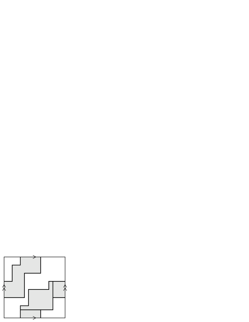
Figure 7. Cutting the annulus $F$ into two discs $F_{1}$ and $F_{2}$

∎

Lemma 4.3.

Let $R$ and $R^{\prime}$ be rectangular diagrams of a link such that:

1. $\Gamma_{\overrightarrow{\mathrm{II}}}(R)$ and $\Gamma_{\overrightarrow{\mathrm{II}}}(R^{\prime})$ have the same set of double points, which we denote by $X$;

2. there is an isotopy from $\Gamma_{\overrightarrow{\mathrm{II}}}(R)$ to $\Gamma_{\overrightarrow{\mathrm{II}}}(R^{\prime})$ in $\mathbb{T}^{2}$ fixed on an open neighborhood of $X$.

Then $[R]_{\overrightarrow{\mathrm{II}}}=[R^{\prime}]_{\overrightarrow{\mathrm{II}}}$.

Proof.

As before, we put $\Gamma=\Gamma_{\overrightarrow{\mathrm{II}}}(R)$ and $\Gamma^{\prime}=\Gamma_{\overrightarrow{\mathrm{II}}}(R^{\prime})$ and assume that no longitude or meridian contains four points of $R\cup R^{\prime}$.

The closure $\alpha$ of a connected component of $\Gamma\setminus X$ (respectively, $\Gamma^{\prime}\setminus X$) will be called an arc of $\Gamma$ (respectively, $\Gamma^{\prime}$) if $\alpha\cap X\neq\varnothing$. There is a natural one-to-one correspondence between the arcs of $\Gamma$ and those of $\Gamma^{\prime}$, defined by demanding that arcs $\alpha\subset\Gamma$ and $\alpha^{\prime}\subset\Gamma^{\prime}$ corresponding to each other have the same starting (equivalently, terminal) portion. Let $\alpha_{1},\alpha_{2},\ldots,\alpha_{N}$ be all the arcs of $\Gamma$, and let $\alpha_{1}^{\prime},\alpha_{2}^{\prime},\ldots,\alpha_{N}^{\prime}$ be the respective arcs of $\Gamma^{\prime}$.

Some connected components of $\Gamma$ (and hence of $\Gamma^{\prime}$) may be disjoint from $X$, and thus be simple closed staircase-like curves, which are pairwise disjoint and homologous to each other. Let $\gamma_{1},\gamma_{2},\ldots,\gamma_{K}$ be all these components numbered using the following recipe. Choose a point $x_{0}\in X$ if $X$ is non-empty, and $x_{0}\in\mathbb{T}^{2}\setminus(\Gamma\cup\Gamma^{\prime})$ otherwise. Choose also an oriented loop $\beta\subset\mathbb{T}^{2}$ based at $x_{0}$ that intersects each $\gamma_{i}$ exactly once. The numbering of $\gamma_{i}$’s is chosen according to the order in which the points $\gamma_{i}\cap\beta$ follow on $\beta$.

Let $\gamma_{1}^{\prime},\gamma_{2}^{\prime},\ldots,\gamma_{K}^{\prime}$ be the closed components of $\Gamma^{\prime}\setminus X$ numbered so that an isotopy bringing $\Gamma$ to $\Gamma^{\prime}$ and fixed on $X\cup\{x_{0}\}$ brings $\gamma_{i}$ to $\gamma_{i}^{\prime}$, $i=1,\ldots,K$.

We proceed by induction in

(2) $$c(R,R^{\prime})=(K+1)\Bigl{(}\sum_{\beta,\beta^{\prime}}\chi(\beta\cap\beta^{\prime})-N\Bigr{)}+\bigl{|}\{i=1,\ldots,K:\gamma_{i}\neq\gamma_{i}^{\prime}\}\bigr{|},$$

where $\chi$ denotes the Euler characteristics, and the sum is taken over all connected components $\beta$ of $\Gamma\setminus X$ and all connected components $\beta^{\prime}$ of $\Gamma^{\prime}\setminus X$.

The equality $c(R,R^{\prime})=0$ means that $R$ and $R^{\prime}$ coincide. This is the induction base.

Suppose that $c(R,R^{\prime})>0$ and $\sum_{\beta,\beta^{\prime}}\chi(\beta\cap\beta^{\prime})=N$. This means that all the arcs of $\Gamma^{\prime}$ coincide with the respective arcs of $\Gamma$, and, for any $i,j\in\{1,\ldots,K\}$, the curves $\gamma_{i}$ and $\gamma_{j}^{\prime}$ are either coincident or disjoint.

Let $k$ be the minimal index such that $\gamma_{k}\neq\gamma_{k}^{\prime}$. Then $\gamma_{k}$ and $\gamma_{k}^{\prime}$ cut the torus $\mathbb{T}^{2}$ into two annuli. Let $A$ be the one of these annuli that does not contain the point $x_{0}$. The interior of $A$ is disjoint either from $\Gamma$ or from $\Gamma^{\prime}$. Without loss of generality we may assume the former. There is a rectangular diagram of a link $R^{\prime\prime}$ such that $\Gamma_{\overrightarrow{\mathrm{II}}}(R^{\prime\prime})=(\Gamma\setminus\gamma_{k})\cup\gamma_{k}^{\prime}$. We have $[R]_{\overrightarrow{\mathrm{II}}}=[R^{\prime\prime}]_{\overrightarrow{\mathrm{II}}}$ by Lemma 4.2 and $c(R^{\prime\prime},R^{\prime})<c(R,R^{\prime})$, which gives the induction step.

Now suppose that $\sum_{\beta,\beta^{\prime}}\chi(\beta\cap\beta^{\prime})>N$. This means that, for some $i\in\{1,\ldots,N\}$, we have $\alpha_{i}\neq\alpha_{i}^{\prime}$ or, for some $i,j\in\{1,\ldots,K\}$, we have $\gamma_{i}\cap\gamma_{j}^{\prime}\neq\varnothing$, $\gamma_{i}\neq\gamma_{j}^{\prime}$. In both cases, we claim that either $c(R,R^{\prime})$ can be reduced by a small perturbation of $R$ or $R^{\prime}$ keeping the set of double points of $\Gamma$ fixed, or there is a disc $d\subset\mathbb{T}^{2}$ co-bounded by two staircase arcs $\beta,\beta^{\prime}$ such that

$$d\cap\Gamma=\beta\subset\Gamma\setminus X,\qquad d\cap\Gamma^{\prime}=\beta^{\prime}\subset\Gamma^{\prime}\setminus X.$$

Take this claim for granted for the moment. In the former case, the induction step is obvious. In the latter case, there is a rectangular diagram of a link $R^{\prime\prime}$ such that $\Gamma_{\overrightarrow{\mathrm{II}}}(R^{\prime\prime})=(\Gamma\setminus\beta)\cup\beta^{\prime}$. By Lemma 4.2, for such a diagram, we again have $[R]_{\overrightarrow{\mathrm{II}}}=[R^{\prime\prime}]_{\overrightarrow{\mathrm{II}}}$. The first summand in (2) decreases by $K+1$ when $R$ is replaced by $R^{\prime\prime}$, whereas the second summand may increase by at most $K$ (as a result of possible renumbering of $\gamma_{i}$’s). Hence $c(R^{\prime\prime},R^{\prime})<c(R,R^{\prime})$, and the induction step follows.

Now we prove the claim. A disc in $\mathbb{T}^{2}$ disjoint from $X$ and co-bounded by a subarc of $\Gamma\setminus X$ and a subarc of $\Gamma^{\prime}\setminus X$ will be referred to as a bigon of $\Gamma$ and $\Gamma^{\prime}$. If these subarcs are the only intersections of the bigon with $\Gamma$ and $\Gamma^{\prime}$, then the bigon will be called clean. We use a similar terminology for the full preimages $\widetilde{\Gamma}$ and $\widetilde{\Gamma}^{\prime}$ of $\Gamma$ and $\Gamma^{\prime}$, respectively, under the projection map $\mathbb{R}^{2}\rightarrow\mathbb{T}^{2}=\mathbb{R}^{2}/(2\pi\mathbb{Z}^{2})$. The set of double points of $\widetilde{\Gamma}$ (equivalently, of $\widetilde{\Gamma}^{\prime}$) is denoted by $\widetilde{X}$.

Suppose that $\alpha_{i}\neq\alpha^{\prime}_{i}$ for some $i\in\{1,\ldots,N\}$. Choose preimages $\widetilde{\alpha}_{i}$ and $\widetilde{\alpha}_{i}^{\prime}$ of these arcs in $\mathbb{R}^{2}$ so that $\partial\widetilde{\alpha}_{i}=\partial\widetilde{\alpha}_{i}^{\prime}$. (The arcs $\alpha_{i}$ and $\alpha_{i}^{\prime}$ may form closed loops based at a point from $X$, in which case $\widetilde{\alpha}_{i}$ and $\widetilde{\alpha}_{i}^{\prime}$ are defined as the closures of preimages of $\alpha_{i}\setminus X$ and $\alpha_{i}^{\prime}\setminus X$, such that $\partial\widetilde{\alpha}_{i}=\partial\widetilde{\alpha}_{i}^{\prime}$.)

By the hypothesis of the lemma, the staircase arcs $\widetilde{\alpha}_{i}$ and $\widetilde{\alpha}^{\prime}_{i}$ are isotopic relative to $\widetilde{X}$ and coincide near $\partial\widetilde{\alpha}_{i}=\partial\widetilde{\alpha}_{i}^{\prime}\subset\widetilde{X}$. This implies the existence of a bigon $\widetilde{d}$ of $\widetilde{\Gamma}$ and $\widetilde{\Gamma}^{\prime}$ with $\partial\widetilde{d}\subset\widetilde{\alpha}_{i}\cup\widetilde{\alpha}_{i}^{\prime}$. However, this bigon is not necessarily clean. If the interior of $\widetilde{d}$ has a non-empty intersection with $\widetilde{\Gamma}$ or $\widetilde{\Gamma}^{\prime}$, then a subarc of $\widetilde{\Gamma}\setminus\widetilde{X}$ or $\widetilde{\Gamma}^{\prime}\setminus\widetilde{X}$ cuts off a smaller bigon from $\widetilde{d}$. Let $\widetilde{d}_{0}$ be a minimal bigon of $\widetilde{\Gamma}$ and $\widetilde{\Gamma}^{\prime}$ contained in $\widetilde{d}$, that is, such that there is no smaller bigon contained in $\widetilde{d}_{0}$.

Let $\widetilde{\beta}\subset\widetilde{\Gamma}\setminus\widetilde{X}$ and $\widetilde{\beta}^{\prime}\subset\widetilde{\Gamma}^{\prime}\setminus\widetilde{X}$ be the arcs co-bounding $\widetilde{d}_{0}$. By construction, the interior of $\widetilde{d}_{0}$ is disjoint from $\widetilde{\Gamma}$ and $\widetilde{\Gamma}^{\prime}$. If $\widetilde{\beta}$ has a non-empty intersection with $\widetilde{\Gamma}^{\prime}$, or $\widetilde{\beta}^{\prime}$ has a non-empty intersection with $\widetilde{\Gamma}$, then this intersection can be resolved by a small perturbation of $R$ or $R^{\prime}$, which results in decreasing of $c(R,R^{\prime})$. If $\beta\cap\Gamma^{\prime}=\varnothing=\beta^{\prime}\cap\Gamma$, then the bigon $\widetilde{d}_{0}$ is clean, and so is its image $d_{0}$ in $\mathbb{T}^{2}$. The claim follows.

Now suppose that $\alpha_{i}=\alpha_{i}^{\prime}$ for all $i=1,\ldots,N$. Let $i,j\in\{1,\ldots,K\}$ be such that $\gamma_{i}\cap\gamma_{j}^{\prime}\neq\varnothing$, $\gamma_{i}\neq\gamma_{j}^{\prime}$. If $\gamma_{i}\cap\gamma_{j}^{\prime}$ is a single point, this intersection can be resolved by a small perturbation of $R$ or $R^{\prime}$, which results in decreasing of $c(R,R^{\prime})$. Otherwise we find a bigon $\widetilde{d}$ of $\widetilde{\Gamma}$ and $\widetilde{\Gamma}^{\prime}$ co-bounded by some $\beta\subset\widetilde{\gamma}_{i}$ and $\beta^{\prime}\subset\widetilde{\gamma}_{j}^{\prime}$, where $\widetilde{\gamma}_{i}$ and $\widetilde{\gamma}_{j}^{\prime}$ are preimages of $\gamma_{i}$ and $\gamma_{j}^{\prime}$, respectively, in $\mathbb{R}^{2}$, and proceed as above. ∎

Proof of Theorem 4.1.

Due to symmetry it suffices to prove the assertion for any of the four types of stabilizations. We choose $T=\overrightarrow{\mathrm{II}}$.

Two rectangular diagrams of a link $R$ and $R^{\prime}$ (or, more generally, any two pairs $(R^{+},R^{-})$, $({R^{\prime}}^{+},{R^{\prime}}^{-})$ of finite subsets of $\mathbb{T}^{2}$) are called combinatorially equivalent if there are orientation-preserving self-homeomorphisms $f,g$ of $\mathbb{S}^{1}$ such that $(f\times g)(R^{\pm})={R^{\prime}}^{\pm}$.

Two rectangular diagrams of a link $R$ and $R^{\prime}$ are said to be of the same $\overrightarrow{\mathrm{II}}$-homology type if there is a rectangular diagram of a link $R^{\prime\prime}$ such that $R^{\prime}$ and $R^{\prime\prime}$ are combinatorially equivalent, and $\Gamma=\Gamma_{\overrightarrow{\mathrm{II}}}(R)$ is isotopic to $\Gamma_{\overrightarrow{\mathrm{II}}}(R^{\prime\prime})$ relative to the set of double points of $\Gamma$. This is clearly an equivalence relation. It follows from Lemma 4.3 that the coincidence of the $\overrightarrow{\mathrm{II}}$-homology types of $R$ and $R^{\prime}$ implies $[R]_{\overrightarrow{\mathrm{II}}}=[R^{\prime}]_{\overrightarrow{\mathrm{II}}}$.

Remark 4.1.

The term ‘homology type’ is justified by the fact that the $\overrightarrow{\mathrm{II}}$-homology type of a diagram $R$ is determined by the homological information about $\Gamma_{\overrightarrow{\mathrm{II}}}(R)$, which can be encoded by the function $\psi:H_{1}(\Gamma,X;\mathbb{Z})\rightarrow\mathbb{Z}$ defined by

$$\psi(z)=\bigl{|}\{\alpha\subset\Gamma\setminus X:[\overline{\alpha}]=z\}\bigr{|},$$

where $\Gamma=\Gamma_{\overrightarrow{\mathrm{II}}}(R)$, and $X$ is the set of double points of $\Gamma$.

Now we claim that, for any $k,l\in\mathbb{N}$ and $m\in\mathbb{N}\cup\{0\}$, there are only finitely many pairwise distinct $\overrightarrow{\mathrm{II}}$-homology types of diagrams $R$ such that $\omega_{\overrightarrow{\mathrm{II}}}(R)=(k,l,m)$.

Indeed, if $\omega_{\overrightarrow{\mathrm{II}}}(R)=(k,l,0)$, then $\Gamma_{\overrightarrow{\mathrm{II}}}(R)$ is a union of $\mathrm{lcd}(k,l)$ simple closed curves in $\mathbb{T}^{2}$ having homology class $(k,l)/\mathrm{lcd}(k,l)$. This means that the $\overrightarrow{\mathrm{II}}$-homology type is completely determined by $k,l$.

Suppose $\omega_{\overrightarrow{\mathrm{II}}}(R)=(k,l,m)$ with $m>0$. Denote by $X$ the set of double points of $\Gamma=\Gamma_{\overrightarrow{\mathrm{II}}}(R)$. Let $\theta_{1},\theta_{2},\ldots,\theta_{K}\in\mathbb{S}^{1}$ (respectively, $\varphi_{1},\varphi_{2},\ldots,\varphi_{L}\in\mathbb{S}^{1}$) be all the points in the projection $p_{\theta}(X)$ (respectively, $p_{\varphi}(X)$) numbered according to their cyclic order in $\mathbb{S}^{1}$. We have $K,L\leqslant m$.

Pick an $\varepsilon>0$ smaller than one half of the length of the shortest interval among those into which $\mathbb{S}^{1}$ is cut by $p_{\theta}(R)\cup p_{\varphi}(R)$. Then whenever $(\theta_{i},\varphi_{j})\in X$, we will have

(3) $$\Gamma\cap[\theta_{i}-\varepsilon;\theta_{i}+\varepsilon]\times[\varphi_{j}-\varepsilon;\varphi_{j}+\varepsilon]=\bigl{(}[\theta_{i}-\varepsilon;\theta_{i}+\varepsilon]\times\{\varphi_{j}\}\bigr{)}\cup\bigl{(}\{\theta_{i}\}\times[\varphi_{j}-\varepsilon;\varphi_{j}+\varepsilon]\bigr{)}.$$

Denote the set $\bigcup_{i=1}^{K}\{\theta_{i}-\varepsilon,\theta_{i}+\varepsilon\}\subset\mathbb{S}^{1}$ by $\Theta$ and $\bigcup_{j=1}^{L}\{\varphi_{j}-\varepsilon,\varphi_{j}+\varepsilon\}\subset\mathbb{S}^{1}$ by $\Phi$. Due to the choice of $\varepsilon$, we have $\Theta\cap p_{\theta}(R)=\varnothing=\Phi\cap p_{\varphi}(R)$ since $p_{\theta}(X)\subset p_{\theta}(R)$ and $p_{\varphi}(X)\subset p_{\varphi}(R)$. Therefore, whenever $\theta_{0}\in\Theta$ (respectively, $\varphi_{0}\in\Phi$), the meridian $\{\theta_{0}\}\times\mathbb{S}^{1}$ (respectively, the longitude $\mathbb{S}^{1}\times\{\varphi_{0}\}$) intersects $\Gamma$ in exactly $k$ (respectively, $l$) points.

Denote by $Y$ the set of all such intersection points:

$$Y=\bigl{(}(\Theta\times\mathbb{S}^{1})\cup(\mathbb{S}^{1}\times\Phi)\bigr{)}\cap\Gamma.$$

We claim that the homology type of $R$ can be recovered from $X$ and $Y$. Indeed, we can recover the subsets $\Theta$ and $\Phi$ as they are the projections $p_{\theta}(Y)$ and $p_{\varphi}(Y)$.

Now let $r$ be the closure of a connected component of $\mathbb{T}^{2}\setminus\bigl{(}(\Theta\times\mathbb{S}^{1})\cup(\mathbb{S}^{1}\times\Phi)\bigr{)}$. By construction, $r$ is a rectangle which is either disjoint from $X$ or contains exactly one point from $X$. In the former case, we can recover $\Gamma\cap r$ up to isotopy relative to $\partial r$ since $\partial r\cap\Gamma\subset Y$ and $\Gamma\cap r$ is a union of pairwise disjoint staircase arcs on which the functions $\theta$, $\varphi$ are non-decreasing (some of these arcs may be degenerate to a single point). In the latter case, the intersection $\Gamma\cap r$ is completely known due to (3).

The number of points in $Y$ is bounded from above by a function of $k,l,m$:

$$|Y|=2Kk+2Ll\leqslant 2m(k+l).$$

Therefore, for any fixed triple $(k,l,m)$ there are only finitely many combinatorial types of pairs $(X,Y)$ that can arise in this construction, and hence, the number of homology types or rectangular diagrams $R$ with $\omega_{\overrightarrow{\mathrm{II}}}(R)=(k,l,m)$ is also finite.

In a similar fashion one can show that, for any fixed triple $(k,l,m)$, the number of pairs of homology types $(Z,Z^{\prime})$ of rectangular diagrams such that, for some  $R\in Z$, $R^{\prime}\in Z^{\prime}$, we have $\omega_{\overrightarrow{\mathrm{II}}}(R)=\omega_{\overrightarrow{\mathrm{II}}}(R^{\prime})=(k,l,m)$ and $R\mapsto R^{\prime}$ is either an exchange move or a type $\overrightarrow{\mathrm{II}}$ stabilization, is also finite.

Thus, an algorithm to decide wether $[R]_{\overrightarrow{\mathrm{II}}}=[R^{\prime}]_{\overrightarrow{\mathrm{II}}}$ is constructed as follows. First, compute $\omega_{\overrightarrow{\mathrm{II}}}(R)$ and $\omega_{\overrightarrow{\mathrm{II}}}(R^{\prime})$. If $\omega_{\overrightarrow{\mathrm{II}}}(R)\neq\omega_{\overrightarrow{\mathrm{II}}}(R^{\prime})$, then $[R]_{\overrightarrow{\mathrm{II}}}\neq[R^{\prime}]_{\overrightarrow{\mathrm{II}}}$ by Lemma 4.1.

If $\omega_{\overrightarrow{\mathrm{II}}}(R)=\omega_{\overrightarrow{\mathrm{II}}}(R^{\prime})=(k,l,m)$ we construct a graph $G$ whose vertices are homology types of all rectangular diagrams of links $R^{\prime\prime}$ with $\omega_{\overrightarrow{\mathrm{II}}}(R^{\prime\prime})=(k,l,m)$, and the edges are all pairs $(Z_{1},Z_{2})$ of vertices such that there exists an exchange move or a type $\overrightarrow{\mathrm{II}}$ stabilization $R_{1}\mapsto R_{2}$ with $R_{1}\in Z_{1}$, $R_{2}\in Z_{2}$. As we have seen above, this graph is finite. It is also clear that a procedure to construct this graph as well as to find its vertices $Z$, $Z^{\prime}$ with $Z\ni R$ and $Z^{\prime}\ni R^{\prime}$ can be described in a purely combinatorial way. Now the equality $[R]_{\overrightarrow{\mathrm{II}}}=[R^{\prime}]_{\overrightarrow{\mathrm{II}}}$ holds if and only if the vertices $Z$ and $Z^{\prime}$ belong to the same connected component of $G$, which is easily checkable. ∎

Corollary 4.1.

The equivalence problem for transverse links of a topological type that has trivial orientation-preserving symmetry group is decidable.

Proof.

Recall that equivalence classes of positively $\xi_{+}$-transverse links can be viewed as $\xi_{+}$-Legendrian links modulo Legendrian isotopy and negative stabilizations, and also as elements of $\mathscr{R}/\bigl{\langle}\overrightarrow{\mathrm{I}},\overleftarrow{\mathrm{I}},\overrightarrow{\mathrm{II}}\bigr{\rangle}$, whereas equivalence classes of $\xi_{+}$-Legendrian (respectively, $\xi_{-}$-Legendrian) links are identified with elements of $\mathscr{R}/\langle\overrightarrow{\mathrm{I}},\overleftarrow{\mathrm{I}}\rangle$ (respectively, $\mathscr{R}/\langle\overrightarrow{\mathrm{II}},\overleftarrow{\mathrm{II}}\rangle$) (see [7, 10]).

The proof of the corollary is parallel to that of [7, Theorem 7.1]. Namely, for any two topologically equivalent positively $\xi_{+}$-transverse links we can find their presentations by rectangular diagrams $R_{1}$, $R_{2}$ such that $[R_{1}]_{\overrightarrow{\mathrm{II}},\overleftarrow{\mathrm{II}}}=[R_{2}]_{\overrightarrow{\mathrm{II}},\overleftarrow{\mathrm{II}}}$. If the links $\widehat{R}_{1}$ and $\widehat{R}_{2}$ have trivial orientation-preserving symmetry group, then by [7, Theorem 4.2], we have

$$[R_{1}]_{\overrightarrow{\mathrm{II}}}=[R_{2}]_{\overrightarrow{\mathrm{II}}}\quad\Leftrightarrow\quad[R_{1}]_{\overrightarrow{\mathrm{I}},\overleftarrow{\mathrm{I}},\overrightarrow{\mathrm{II}}}=[R_{2}]_{\overrightarrow{\mathrm{I}},\overleftarrow{\mathrm{I}},\overrightarrow{\mathrm{II}}}.$$

An application of Theorem 4.1 completes the proof. ∎

5. Transverse–Legendrian links

For an introduction to contact topology and the theory of Legendrian and transverse knots the reader is referred to [8] and [9]. Here we consider links which are Legendrian with respect to one contact structure and transverse to another, simultaneously.

Namely, let $\xi_{+}$ and $\xi_{-}$ be the cooriented contact structures on $\mathbb{S}^{3}$ defined by the $1$-forms

$$\alpha_{+}=\sin^{2}\Bigl{(}\frac{\pi\tau}{2}\Bigr{)}\,d\theta+\cos^{2}\Bigl{(}\frac{\pi\tau}{2}\Bigr{)}\,d\varphi\qquad\text{and}\qquad\alpha_{-}=\sin^{2}\Bigl{(}\frac{\pi\tau}{2}\Bigr{)}\,d\theta-\cos^{2}\Bigl{(}\frac{\pi\tau}{2}\Bigr{)}\,d\varphi,$$

respectively, that is $\xi_{\pm}=\ker\alpha_{\pm}$. One can see that $\xi_{+}$ is nothing else but the standard contact structure, and $\xi_{-}$ is a mirror image of $\xi_{+}$.

Definition 5.1.

A smooth link in $\mathbb{S}^{3}$ is called transverse-Legendrian of type $\overrightarrow{\mathrm{II}}$ (or simply transverse-Legendrian) if it is positively transverse with respect to $\xi_{+}$ and Legendrian with respect to $\xi_{-}$.

Two transverse-Legendrian links are equivalent if they are isotopic within the class of transverse-Legendrian links.

Let $L$ be a transverse-Legendrian link. The contact structures $\xi_{+}$ and $\xi_{-}$ agree, if their coorientations are ignored, at the union $\mathbb{S}^{1}_{\tau=0}\cup\mathbb{S}^{1}_{\tau=1}$, since we have $\alpha_{+}=\pm\alpha_{-}$ on this subset. Therefore, $L$ misses the circles $\mathbb{S}^{1}_{\tau=0}$ and $\mathbb{S}^{1}_{\tau=1}$, and the torus projection $p_{\theta,\varphi}$ is well defined on the whole of $L$. One can also see that the restriction of both forms $d\theta$ and $d\varphi$ on $L$ are non-degenerate and, moreover, positive with respect to the orientation of $L$.

Any transverse-Legendrian link $L$ can be uniquely recovered from its torus projection similarly to the way in which a Legendrian link is recovered from its front projection. Indeed, since $\alpha_{-}|_{L}=0$, the following equality holds for the restrictions of the coordinates $\theta,\varphi,\tau$ on $L$:

(4) $$\tau=\frac{2}{\pi}\sqrt{\arctan\frac{d\varphi}{d\theta}}.$$

This means that we can describe the set of transverse-Legendrian links completely in terms of torus projections. Namely, the following statement holds:

Proposition 5.1.

The torus projection map gives rise to a one-to-one correspondence between transverse-Legendrian links and subsets $\Gamma\subset\mathbb{T}^{2}$ such that the following holds:

1. $\Gamma$ is the image of a smooth immersion $\mathbb{S}^{1}\sqcup\mathbb{S}^{1}\sqcup\ldots\sqcup\mathbb{S}^{1}\rightarrow\mathbb{T}^{2}$,

2. the slope of $\Gamma$ is everywhere positive, and

3. $\Gamma$ has no self-tangencies.

A subset satisfying Conditions 1–3 of this proposition will be referred as a (positive) torus front.

A torus front is said to be almost generic if it has no self-intersections of multiplicity higher than two, and generic if, additionally, no meridian or longitude of $\mathbb{T}^{2}$ contains more than one self-intersection points of the front. An example of a generic torus front is shown in Figure 8.

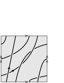
Figure 8. A generic positive torus front

We use a convention that, at every crossing point, the arc with with larger slope is shown as overcrossing. Due to (4), this agrees with the position of the corresponding transverse-Legendrian link in $\mathbb{S}^{3}$. We also indicate the orientation of the corresponding transverse-Legendrian link.

Proposition 5.2.

Two almost generic torus fronts define equivalent transverse-Legendrian links if and only if they are obtained from one another by a sequence of continuous deformations in the class of almost generic torus fronts, and type III Reidemeister moves.

Proof.

This follows from the obvious fact that the main, codimension-one stratum of the set of non-almost generic torus fronts consists of torus fronts having a triple self-intersection point. ∎

With every rectangular diagram of a link $R$ we associate an equivalence class $\mathrm{TL}_{\overrightarrow{\mathrm{II}}}(R)$ of transverse-Legendrian links by demanding that a torus front representing an element of $\mathrm{TL}_{\overrightarrow{\mathrm{II}}}(R)$ can be obtained by an arbitrarily small (in the $C^{0}$ sense) perturbation of $\Gamma_{\overrightarrow{\mathrm{II}}}(R)$.

$\Gamma_{\overrightarrow{\mathrm{II}}}(R)$		torus projection of $\mathrm{TL}_{\overrightarrow{\mathrm{II}}}(R)$

Figure 9. Producing a transverse-Legendrian link from a rectangular diagram of a link

See Figure 9 for an example.

Proposition 5.3.

(i) Every equivalence class of type $\overrightarrow{\mathrm{II}}$ transverse-Legendrian links has the form $\mathrm{TL}_{\overrightarrow{\mathrm{II}}}(R)$ for some rectangular diagram of a link $R$.

(ii) Let $R$ and $R^{\prime}$ be rectangular diagrams of a link. Then $\mathrm{TL}_{\overrightarrow{\mathrm{II}}}(R)=\mathrm{TL}_{\overrightarrow{\mathrm{II}}}(R^{\prime})$ implies $[R]_{\overrightarrow{\mathrm{II}}}=[R^{\prime}]_{\overrightarrow{\mathrm{II}}}$.

Proof.

Statement (i) follows from the approximation argument: any generic positive torus front $\Gamma$ can be approximated by a union of immersed staircase-like closed curves of the form $\Gamma_{\overrightarrow{\mathrm{II}}}(R)$, where $R$ is a rectangular diagram of a surface, so that $\Gamma_{\overrightarrow{\mathrm{II}}}(R)$ and $\Gamma$ have the same set of double points.

To prove statement (ii), let $\Gamma$ and $\Gamma^{\prime}$ be generic torus fronts obtained from $\Gamma_{\overrightarrow{\mathrm{II}}}(R)$ and $\Gamma_{\overrightarrow{\mathrm{II}}}(R^{\prime})$, respectively, by a $C^{0}$-small perturbation. The equality $\mathrm{TL}_{\overrightarrow{\mathrm{II}}}(R)=\mathrm{TL}_{\overrightarrow{\mathrm{II}}}(R^{\prime})$ means that there is a continuous $1$-parametric family $\Gamma_{t}$, $t\in[0;1]$ of torus fronts such that $\Gamma_{0}=\Gamma$, $\Gamma_{1}=\Gamma^{\prime}$. Such a family can be chosen so that there are only finitely many moments $t=t_{1},t_{2},\ldots,t_{m}$ at which the torus front $\Gamma_{t}$ is not generic, and at these moments the genericity of $\Gamma_{t}$ is unavoidably broken in one of the two simplest ways: either there are two double points of $\Gamma_{t}$ at the same meridian or longitude, or $\Gamma_{t}$ has a triple self-intersection. We may assume that $t_{1}<t_{2}<\ldots<t_{m}$. We also set $t_{0}=0$, $t_{m+1}=1$.

For each $t\in[0;1]\setminus\{t_{1},\ldots,t_{m}\}$ let $R_{t}$ be a rectangular diagram of a link such that $\Gamma_{\overrightarrow{\mathrm{II}}}(R_{t})$ is isotopic to $\Gamma_{t}$ relative the set of self-intersections of $\Gamma_{t}$. By construction, the homology type of $R_{t}$ is constant on each of the intervals $[0;t_{1})$, $(t_{1};t_{2}),\ldots$, $(t_{m-1};t_{m})$, $(t_{m};1]$, and thus, by Lemma 4.3, so is $[R_{t}]_{\overrightarrow{\mathrm{II}}}$. At any critical moment $t_{i}$ the torus front $\Gamma_{t_{i}}$ can be approximated in two different ways by unions of staircase curves $\Gamma_{\overrightarrow{\mathrm{II}}}(R_{t_{i}}^{\prime})$ and $\Gamma_{\overrightarrow{\mathrm{II}}}(R_{t_{i}}^{\prime\prime})$, where $R_{t_{i}}^{\prime}$ and $R_{t_{i}}^{\prime\prime}$ are rectangular diagrams of a link such that:

1. $R_{t_{i}}^{\prime-}\mapsto R_{t_{i}}^{\prime\prime}$ is an exchange move;

2. the homology type of $R_{t_{i}}^{\prime}$ (respectively, $R_{t_{i}}^{\prime\prime}$) coincides with that of $R_{t}$ for $t\in(t_{i-1};t_{i})$ (respectively, $t\in(t_{i};t_{i+1})$).

This is illustrated in Figure 10.

(a)
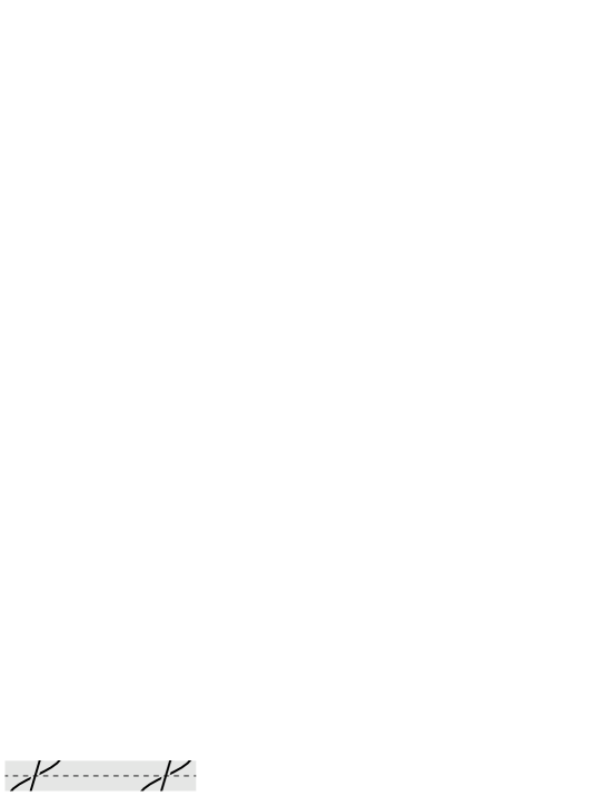
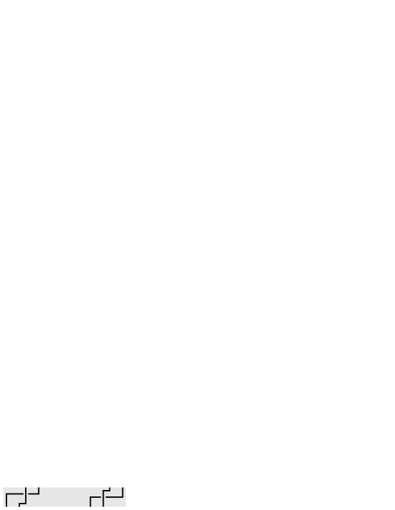
	$\Gamma_{t_{i}}$	$\Gamma_{\overrightarrow{\mathrm{II}}}(R_{t_{i}}^{\prime})$	$\Gamma_{\overrightarrow{\mathrm{II}}}(R_{t_{i}}^{\prime\prime})$
(b)
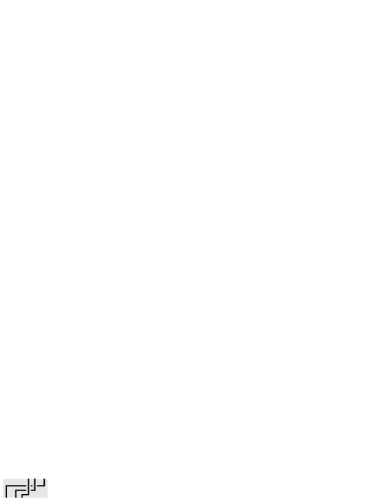
	$\Gamma_{t_{i}}$	$\Gamma_{\overrightarrow{\mathrm{II}}}(R_{t_{i}}^{\prime})$	$\Gamma_{\overrightarrow{\mathrm{II}}}(R_{t_{i}}^{\prime\prime})$

Figure 10. Approximating a non-generic torus front: (a) when two double points appear on the same longitude; (b) when a triple self-intersection occurs

The claim follows. ∎

The converse to the assertion (ii) of Proposition 5.3 does not hold in general. Namely, the equality $[R]_{\overrightarrow{\mathrm{II}}}=[R^{\prime}]_{\overrightarrow{\mathrm{II}}}$ does not always imply $\mathrm{TL}_{\overrightarrow{\mathrm{II}}}(R)=\mathrm{TL}_{\overrightarrow{\mathrm{II}}}(R^{\prime})$. However, the elements of $\mathscr{R}/\bigl{\langle}\overrightarrow{\mathrm{II}}\bigr{\rangle}$ can be classified in terms of transverse-Legendrian links and exchange moves, which we now define.

Definition 5.2.

Let $\Gamma$ and $\Gamma^{\prime}$ be two generic positive torus fronts such that there are three smooth arcs $\alpha\subset\Gamma$, $\alpha^{\prime}\subset\Gamma^{\prime}$, and $\beta\subset\Gamma\cap\Gamma^{\prime}$ satisfying the following conditions (see Figure 11):

1. the closure of the symmetric difference $\Gamma\triangle\Gamma^{\prime}$ is $\alpha\cup\alpha^{\prime}$;

2. there is an embedded closed $2$-disc $d\subset\mathbb{T}^{2}$ such $\partial d=\alpha\cup\alpha^{\prime}$;

3. $\partial\beta\subset\partial d$;

4. $\int_{\beta}d\theta<2\pi$, $\int_{\beta}d\varphi<2\pi$;

5. $\beta$ is homologous, relative to $d$, either to a meridian or to a longitude of $\mathbb{T}^{2}$;

6. the intersection $\beta\cap d$ consists of two arcs $\gamma$ and $\gamma^{\prime}$ such that $\partial\gamma\subset\alpha$, $\partial\gamma^{\prime}\subset\alpha^{\prime}$;

7. the interior of $d$ intersects $\Gamma\setminus\beta$ (equivalently, $\Gamma^{\prime}\setminus\beta$) in a union of pairwise disjoint open arcs each of which separates $\gamma\setminus\partial\gamma$ from $\gamma^{\prime}\setminus\partial\gamma^{\prime}$;

8. if $\beta$ is homologous to a meridian (respectively, longitude) relative to $d$, then at each self-intersection point of $\Gamma$ or $\Gamma^{\prime}$ located at $\partial d\setminus\beta$ the overpassing (respectively, underpassing) arc is a part of $\partial d$.

Then we say that the passage from $\Gamma$ to $\Gamma^{\prime}$ (or between the respective transverse-Legendrian links) is called an exchange move.

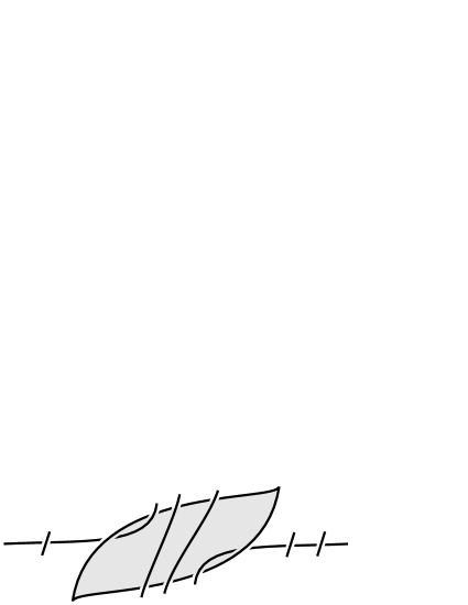
Figure 11. The disc $d$ and the arcs $\alpha,\beta$ in the definition of an exchange move of transverse-Legendrian links

Exchange moves of transverse-Legendrian links are illustrated in Figure 12.

         $\longleftrightarrow$         

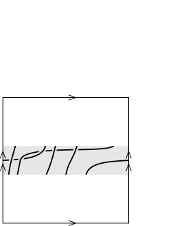
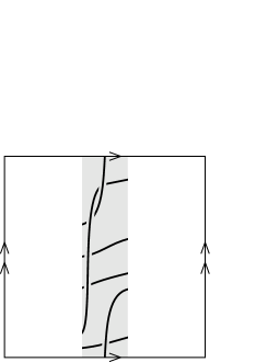
         $\longleftrightarrow$         

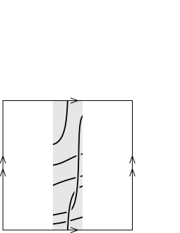
Figure 12. Exchange moves of transverse-Legendrian links

Proposition 5.4.

Let $R$ and $R^{\prime}$ be rectangular diagrams of a link. Then we have $[R]_{\overrightarrow{\mathrm{II}}}=[R^{\prime}]_{\overrightarrow{\mathrm{II}}}$ if and only if the type $\overrightarrow{\mathrm{II}}$ transverse-Legendrian link associated with $R$ and $R^{\prime}$ can be obtained from one another by a finite sequence of isotopies in the class of transverse-Legendrian links, and exchange moves.

Proof.

Due to Proposition 5.3, proving the ‘if’ part amounts to checking that exchange moves of transverse-Legendrian links can be realized my means of elementary moves of respective rectangular diagrams. We leave this to the reader, and don’t use in the sequel.

To prove the ‘only if’ part, first, note that every elementary move of rectangular diagrams can be decomposed into a sequence of ‘even more elementary’ ones, namely, such that each of the annuli $(\theta_{1};\theta_{2})\times\mathbb{S}^{1}$ and $\mathbb{S}^{1}\times(\varphi_{1};\varphi_{2})$ (we use the notation from Definition 3.2) contains at most one edge or the diagram being transformed. This follows from the fact that a single elementary move associated with the rectangle $[\theta_{1};\theta_{2}]\times[\varphi_{1};\varphi_{2}]$ can be decomposed into two moves associated with rectangles $[\theta_{1};\theta_{3}]\times[\varphi_{1};\varphi_{2}]$ and $[\theta_{3};\theta_{2}]\times[\varphi_{1};\varphi_{2}]$ (respectively, $[\theta_{1};\theta_{2}]\times[\varphi_{1};\varphi_{3}]$ and $[\theta_{1};\theta_{2}]\times[\varphi_{3};\varphi_{2}]$) for any $\theta_{3}\in(\theta_{1};\theta_{2})$ (respectively, $\varphi_{3}\in(\varphi_{1};\varphi_{2})$) such that the meridian $\{\theta_{2}\}\times\mathbb{S}^{1}$ (respectively, the longitude $\mathbb{S}^{1}\times\{\varphi_{3}\}$) contains no vertices of the diagram.

In each case of an ‘even more elementary’ move (there are now only finitely many to consider), it is a direct check that the corresponding transverse-Legendrian link undergoes an isotopy in the class of transverse-Legendrian links, possibly composed with an exchange move. ∎

6. Applications

Corollary 4.1 gives a theoretical solution of the equivalence problem for transverse links having trivial orientation-preserving symmetry group, but an implementation of the algorithm takes a lot of time in general. However, the results of [6, 7] supplemented by Propositions 5.2 and 5.4 above allow, in some cases, to distinguish transverse knots having trivial orientation-preserving symmetry group with very little effort. To illustrate this, we consider the knots $10_{128}$ and $10_{160}$.

It is conjectured in [2] chat the $\xi_{+}$-Legendrian knots associated with the rectangular diagrams $10_{128}^{1\mathrm{R}}$ and $-\mu(10_{128}^{1\mathrm{R}})$ shown in Figure 13 (we use the notation of [7] for these diagrams)

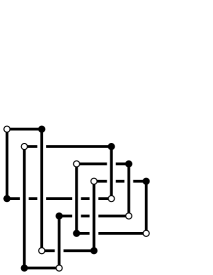
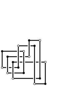
$10_{128}^{1\mathrm{R}}$		$-\mu(10_{128}^{1\mathrm{R}})$

Figure 13. The diagrams $10_{128}^{1\mathrm{R}}$ and $-\mu(10_{128}^{1\mathrm{R}})$

are not Legendrian isotopic, and, moreover, remain such after any number of negative stabilizations. This is equivalent to saying that the positively $\xi_{+}$-transverse knots associated with these diagrams are not transversely isotopic. In the notation introduced in the beginning of this paper, this inequality can also be written as

(5) $$[10_{128}^{1\mathrm{R}}]_{\overrightarrow{\mathrm{I}},\overleftarrow{\mathrm{I}},\overrightarrow{\mathrm{II}}}\neq[-\mu(10_{128}^{1\mathrm{R}})]_{\overrightarrow{\mathrm{I}},\overleftarrow{\mathrm{I}},\overrightarrow{\mathrm{II}}}.$$

This conjecture was partially confirmed in [7, Proposition 7.5], namely, it was shown that the Legendrian knots in questions are, indeed, not equivalent, and remain such after up to four negative stabilizations. Extending this to any number of negative stabilizations now amounts to showing that

(6) $$[10_{128}^{1\mathrm{R}}]_{\overrightarrow{\mathrm{II}}}\neq[-\mu(10_{128}^{1\mathrm{R}})]_{\overrightarrow{\mathrm{II}}}.$$

The type $\overrightarrow{\mathrm{II}}$ transverse-Legendrian knots associated with the diagrams $10_{128}^{1\mathrm{R}}$ and $-\mu(10_{128}^{1\mathrm{R}})$ are shown in Figure 14.

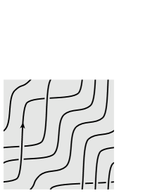
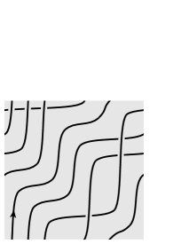
$\mathrm{TL}_{\overrightarrow{\mathrm{II}}}(10_{128}^{1\mathrm{R}})$		$\mathrm{TL}_{\overrightarrow{\mathrm{II}}}(-\mu(10_{128}^{1\mathrm{R}}))$

Figure 14. Torus projections of knots from $\mathrm{TL}_{\overrightarrow{\mathrm{II}}}(10_{128}^{1\mathrm{R}})$ and $\mathrm{TL}_{\overrightarrow{\mathrm{II}}}(-\mu(10_{128}^{1\mathrm{R}}))$

There are no ‘triangles’ in the complement of any of these torus fronts, hence no Reidemeister-III move can be applied to them. It is also not hard to see that these torus fronts admit no exchange moves, even after any isotopy in the class of positive torus fronts, and that they are not isotopic. By Propositions 5.2 and 5.4, this implies (6), and then (5) by [7, Theorem 4.2 and Figure 20].

Thus, we have the following.

Proposition 6.1.

The positively $\xi_{+}$-transverse knots associated with the diagrams $10_{128}^{1\mathrm{R}}$ and $-\mu(10_{128}^{1\mathrm{R}})$ are not transversely isotopic.

In a completely similar fashion the following statement, which also confirms a conjecture of [2], is established.

Proposition 6.2.

The positively $\xi_{+}$-transverse knots associated with the diagrams $-10_{160}^{2\mathrm{R}}$ and $10_{160}^{3\mathrm{R}}$ shown in Figure 15 are not transversely isotopic.

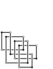
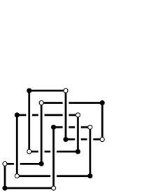
$-10_{160}^{2\mathrm{R}}$		$10_{160}^{3\mathrm{R}}$

Figure 15. The diagrams $-10_{160}^{2\mathrm{R}}$ and $10_{160}^{3\mathrm{R}}$

The proof is obtained by analyzing the torus projections in Figure 16 (see [7, Figure 22] for the notation and a description of the relation between these diagrams and those in [2]).

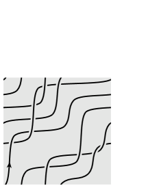
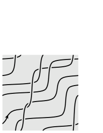
$\mathrm{TL}_{\overrightarrow{\mathrm{II}}}(-10_{160}^{2\mathrm{R}})$		$\mathrm{TL}_{\overrightarrow{\mathrm{II}}}(10_{160}^{3\mathrm{R}})$

Figure 16. Torus projections of $\mathrm{TL}_{\overrightarrow{\mathrm{II}}}(-10_{160}^{2\mathrm{R}})$ and $\mathrm{TL}_{\overrightarrow{\mathrm{II}}}(10_{160}^{3\mathrm{R}})$

7. Concluding remarks

Four oriented types of stabilizations and destabilizations of rectangular diagrams of links are symmetric to each other and play equal roles in knot theory. This means that with every rectangular diagram $R$ of a link one can associate four different objects having the nature of a transverse-Legendrian link type:

• a positively $\xi_{+}$-transverse and $\xi_{-}$-Legendrian link type, which is identified with $[R]_{\overrightarrow{\mathrm{II}}}$,

• a negatively $\xi_{+}$-transverse and $\xi_{-}$-Legendrian link type, which is identified with $[R]_{\overleftarrow{\mathrm{II}}}$,

• a positively $\xi_{-}$-transverse and $\xi_{+}$-Legendrian link type, which is identified with $[R]_{\overrightarrow{\mathrm{I}}}$, and

• a negatively $\xi_{-}$-transverse and $\xi_{+}$-Legendrian link type, which is identified with $[R]_{\overleftarrow{\mathrm{I}}}$.

This is illustrated in Figure 17, where torus projections of all four transverse-Legendrian links are shown.

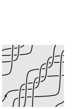
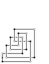
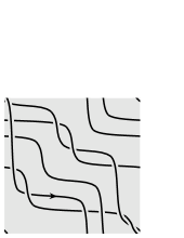
Figure 17. Four transverse-Legendrian links associated with a single rectangular diagram

One may naturally ask if there is a relation between rectangular diagrams and links which are Legendrian with respect to both contact structures $\xi_{+}$ and $\xi_{-}$, or transverse with respect to both of them. The answer in both cases is pretty simple. Links that are $\xi_{+}$-Legendrian and $\xi_{-}$-Legendrian simultaneously are exactly the links of the form $\widehat{R}$, where $R$ is a rectangular diagram of a link (one should extend the definition of a Legendrian link to piecewise smooth curves, since the links of the form $\widehat{R}$ are typically non-smooth). So, equivalence classes of such links are in one-to-one correspondence with combinatorial types of rectangular diagrams.

Links which are positively $\xi_{+}$-transverse and positively $\xi_{-}$-transverse are nothing else but closed braids with $\mathbb{S}^{1}_{\tau=0}$ as the axis. The isotopy classes of such links are the same thing as conjugacy classes of braids. As noted in the beginning of the paper, rectangular diagrams allow to classify braids modulo conjugacy and Birman–Menasco exchange moves (as the elements of $\mathscr{R}/\langle\overrightarrow{\mathrm{I}},\overrightarrow{\mathrm{II}}\rangle$). The situation with transverse-Legendrian links reflected in Proposition 5.4 is completely analogues.

References

- [1] J. Birman, W. Menasco. Studying links via closed braids. IV. Composite links and split links. Invent. Math. 102 (1990), no. 1, 115–139.
- [2] W. Chongchitmate, L. Ng. An atlas of Legendrian knots. Exp. Math. 22 (2013), no. 1, 26–37; arXiv:1010.3997.
- [3] P. Cromwell. Embedding knots and links in an open book. I. Basic properties. Topology Appl. 64 (1995), no. 1, 37–58.
- [4] I. Dynnikov. Arc-presentations of links: Monotonic simplification, Fund.Math. 190 (2006), 29–76; arXiv:math/0208153.
- [5] I. Dynnikov, M. Prasolov. Bypasses for rectangular diagrams. A proof of the Jones conjecture and related questions (Russian), Trudy MMO 74 (2013), no. 1, 115–173; translation in Trans. Moscow Math. Soc. 74 (2013), no. 2, 97–144; arXiv:1206.0898.
- [6] I. Dynnikov, M. Prasolov. Rectangular diagrams of surfaces: distinguishing Legendrian knots. Preprint, arXiv:1712.06366.
- [7] I. Dynnikov, V. Shastin. Distinguishing Legendrian knots with trivial orientation-preserving symmetry group. Preprint, arXiv:1810.06460.
- [8] J. Etnyre. Legendrian and transversal knots. Handbook of knot theory, 105–185, Elsevier B. V., Amsterdam, 2005.
- [9] H. Geiges. An Introduction to Contact Topology, Cambridge University Press (2008).
- [10] P.Ozsváth, Z.Szabó, D.Thurston. Legendrian knots, transverse knots and combinatorial Floer homology, Geometry and Topology, 12 (2008), 941–980, arXiv:math/0611841.