:
\theoremsep
\jmlrvolume1
\jmlryear2019
\jmlrworkshopNeurIPS2019 Disentanglement Challenge
A Preliminary Study of Disentanglement With Insights on the Inadequacy of Metrics
Abstract
Disentangled encoding is an important step towards a better representation learning. However, despite the numerous efforts, there still is no clear winner that captures the independent features of the data in an unsupervised fashion. In this work we empirically evaluate the performance of six unsupervised disentanglement approaches on the mpi3d_toy dataset curated and released for the NeurIPS 2019 Disentanglement Challenge. The methods investigated in this work are -VAE, Factor-VAE, DIP-I-VAE, DIP-II-VAE, Info-VAE, and -TCVAE. The capacities of all models were progressively increased throughout the training and the hyper-parameters were kept intact across experiments. The methods were evaluated based on five disentanglement metrics, namely, DCI, Factor-VAE, IRS, MIG, and SAP-Score. Within the limitations of this study, the -TCVAE approach was found to outperform its alternatives with respect to the normalized sum of metrics. However, a qualitative study of the encoded latents reveal that there is not a consistent correlation between the reported metrics and the disentanglement potential of the model.
keywords:
Disentanglement, Representation Learning, Total Correlation, Factorization1 Introduction
Unsupervised disentanglement is an open problem in the realm of representation learning, incentivized around interpretability (Lake et al., 2016; Bengio et al., 2013). A disentangled representation is a powerful tool in transfer learning, few shot learning, reinforcement learning, and semi-supervised learning of downstream tasks (Goo, 2018; Peters et al., 2017; Bengio et al., 2013).
Here, we compare the disentanglement performance of variational methods. The methods are evaluated based on five relatively established disentanglement metrics on the simplistic rendered images of the mpi3d_toy dataset curated and released for the NeurIPS 2019 Disentanglement Challenge (Gondal et al., 2019).
2 Methods
2.1 Pre-training
To mitigate the sensitivity of the models to the initial state, as suggested by the findings of Goo (2018), an autoencoder model was pre-trained with the conventional VAE objective (Kingma and Welling, 2013) on the mpi3d_toy dataset. This approach guaranteed that models did not collapse into a local minima with little to no reconstruction. It also facilitated the training process given the constraints on the length of training by the challenge.
2.2 Objective Function
In this preliminary study, we implemented the variational objective functions proposed by the following methods: -VAE (Fertig et al., 2018), -TCVAE (Chen et al., 2018), Factor-VAE (Kim and Mnih, 2018), Info-VAE (Zhao et al., 2017), DIP-I-VAE, and DIP-II-VAE (Kumar et al., 2017).
In -TCVAE, the mutual information between the data variables and latent variables are maximized, while the mutual information between the latent variables are minimized. Defining as the th sample of the dataset, the evidence lower bound (ELBO) of this objective can be simplified as follows111The and hyper-parameters of the original formulation are assumed to be 1.
| (1) |
where denotes the th dimension of the latents. In the above equation, the first term is the reconstruction loss. The second term is the distance between the assumed prior distribution of the latent space and the empirical posterior latent distribution. The last term is an indication of the total correlation (TC) between the latent variables which is a generalization of the mutual information for more than two variables (Watanabe, 1960).
2.3 Progressive Capacity Increase
A total capacity constraint which limits the KL divergence between the posterior latent distribution and the factorized prior can encourage the latent representation to be more factorised. However, this will act as an information bottleneck for the reconstruction task and results in a blurry reconstruction. Thus, progressively increasing the information capacity of VAE during training can help facilitate the robust learning of the factorized latents (Burgess et al., 2018). This is achieved by introducing the capacity term and defining the distance between distributions as the absolute deviation from :
| (2) |
Gradually increasing has an annealing effect on the constraint and increases the reconstruction capacity of the model.
3 Experiments and Results
For each learning algorithm, the hyper-parameter sub-spaces were independently searched. However, in order for the results reported here to be comparable, the hyper-parameters were kept intact in between the following experiments.
The input images were pixels and the latent space was of size 20. The model capacity parameter, , was initiated at zero and gradually increased up to 25 over 2000 iterations. Learning rate was initiated at 0.001 and was reduced by a factor of 0.95 when the loss function (\equationrefeq:obj) did not decrease after two consecutive epochs, down to a minimum of 0.0001 . Batch size was set to 64. Optimization was carried out using the Adam optimizer with the default parameters and . The network architectures and other hyper-parameters are detailed in Appendix A.
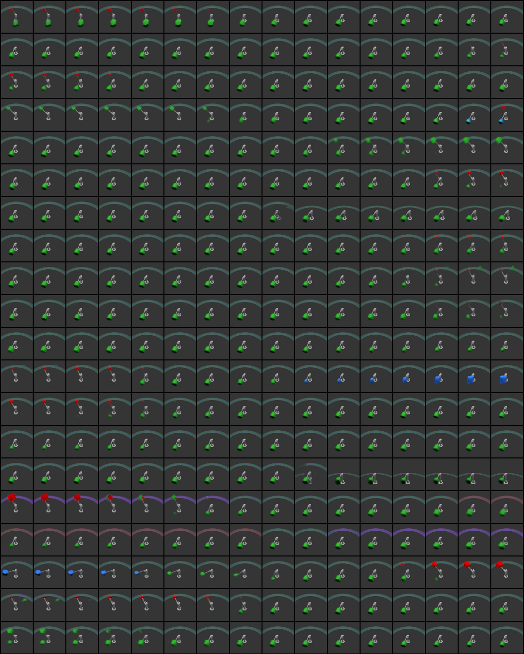
The trained models were evaluated based on five evaluation metrics, namely, DCI, FactorVAE metric, IRS, MIG, and SAP-Score. Results of these evaluations are presented in Table LABEL:tab:results. The non-ignored latent variables of each method are traversed and the results are visualized in Appendix B. Moreover, the evaluation logs during model training are visualized in Appendix C.
All the models and experiments were implemented using the PyTorch deep learning library and packaged under the Disentanglement-PyTorch repository https://github.com/amir-abdi/disentanglement-pytorch.
tab:results Method DCI FactorVAE SAP MIG IRS Normalized Sum -TCVAE 0.392 0.458 0.132 0.203 0.646 4.706 Factor-VAE 0.389 0.449 0.136 0.203 0.577 4.611 -VAE 0.373 0.501 0.135 0.212 0.517 4.599 Info-VAE 0.381 0.523 0.128 0.210 0.514 4.591 DIP-VAE-I 0.385 0.587 0.127 0.188 0.358 4.351 DIP-VAE-II 0.359 0.584 0.111 0.163 0.340 4.023
4 Discussion
In this work we compared the degree of disentanglement in latent encodings of six variational learning algorithms, namely, -VAE, Factor-VAE, DIP-I-VAE, DIP-II-VAE, Info-VAE, and -TCVAE. The empirical results (Table LABEL:tab:results) point to -TCVAE being marginally the superior option and, consequently, chosen as the best performing approach. However, a qualitative study of the traversed latent spaces (Appendix B) reveals that none of the models encoded a true disentangled representation. Lastly, although the DIP-VAE-II model is under performing according to the quantitative results, it has the least number of ignored latent variables with a promising latent traversal compared to other higher performing methods (Appendix B). As a result of these inconsistencies, we find the five metrics utilized in this study inadequate for the purpose of disentanglement evaluation.
Among the limitations of this study is the insufficient search of the hyper-parameters space for all the six learning algorithms. Moreover, the NeurIPS 2019 Disentanglement Challenge imposed an 8-hour limit on the training time of the models which we found to be insufficient. This, while the maximum number of iterations was set to 200k in our experiments, this value was limited to 100k in the submissions made to the challenge portal.
References
- Goo (2018) Challenging Common Assumptions in the Unsupervised Learning of Disentangled Representations, 2018.
- Bengio et al. (2013) Y. Bengio, A. Courville, and P. Vincent. Representation learning: A review and new perspectives. IEEE Transactions on Pattern Analysis and Machine Intelligence, 35(8):1798–1828, August 2013.
- Burgess et al. (2018) Christopher P. Burgess, Irina Higgins, Arka Pal, Loic Matthey, Nick Watters, Guillaume Desjardins, and Alexander Lerchner. Understanding disentangling in -vae, 2018.
- Chen et al. (2018) Ricky T. Q. Chen, Xuechen Li, Roger Grosse, and David Duvenaud. Isolating sources of disentanglement in variational autoencoders, 2018.
- Fertig et al. (2018) Emily Fertig, Aryan Arbabi, and Alexander A. Alemi. -vaes can retain label information even at high compression, 2018.
- Gondal et al. (2019) Muhammad Waleed Gondal, Manuel Wüthrich, Đorđe Miladinović, Francesco Locatello, Martin Breidt, Valentin Volchkov, Joel Akpo, Olivier Bachem, Bernhard Schölkopf, and Stefan Bauer. On the transfer of inductive bias from simulation to the real world: a new disentanglement dataset. arXiv preprint arXiv:1906.03292, 2019.
- Kim and Mnih (2018) Hyunjik Kim and Andriy Mnih. Disentangling by factorising, 2018.
- Kingma and Welling (2013) Diederik P Kingma and Max Welling. Auto-encoding variational bayes, 2013.
- Kumar et al. (2017) Abhishek Kumar, Prasanna Sattigeri, and Avinash Balakrishnan. Variational inference of disentangled latent concepts from unlabeled observations, 2017.
- Lake et al. (2016) Brenden M. Lake, Tomer D. Ullman, Joshua B. Tenenbaum, and Samuel J. Gershman. Building machines that learn and think like people. Behavioral and Brain Sciences, 40, November 2016.
- Peters et al. (2017) Jonas Peters, Dominik Janzing, and Bernhard Schölkopf. Elements of Causal Inference: Foundations and Learning Algorithms. Adaptive Computation and Machine Learning. MIT Press, Cambridge, MA, 2017. ISBN 978-0-262-03731-0.
- Watanabe (1960) Satosi Watanabe. Information theoretical analysis of multivariate correlation. IBM Journal of Research and Development, 4(1):66–82, January 1960.
- Zhao et al. (2017) Shengjia Zhao, Jiaming Song, and Stefano Ermon. Infovae: Information maximizing variational autoencoders, 2017.
Appendix A Model Details
A.1 Architectures of the Neural Networks
The encoder neural network in all experiments consisted of 5 convolutional layers with strides of 2, kernel sizes of , and number of kernels gradually increasing from 32 to 256. The encoder ended with a dense linear layer which estimated the posterior latent distribution as a parametric Gaussian. The decoder network consisted of one convolutional followed with 6 deconvolutional (transposed convolutional) layers, with kernel sizes of 4, strides of 2, and the number of kernels gradually decreasing from 256 down to the number of channels of the image space. ReLU activations were used throughout the architecture, except for the last layers of the encoder and decoder networks.
A.2 Hyper-parameters
tab:specs Method Parameters -TCVAE -VAE Info-VAE DIP-I-VAE DIP-II-VAE Factor-VAE Shared Batch Size=64, LR= by a factor of , C= over 2000 steps, Adam, Adam Latent Size=20, Image Size=
Appendix B Traversed Latent Space of Trained Models
fig:info-vae
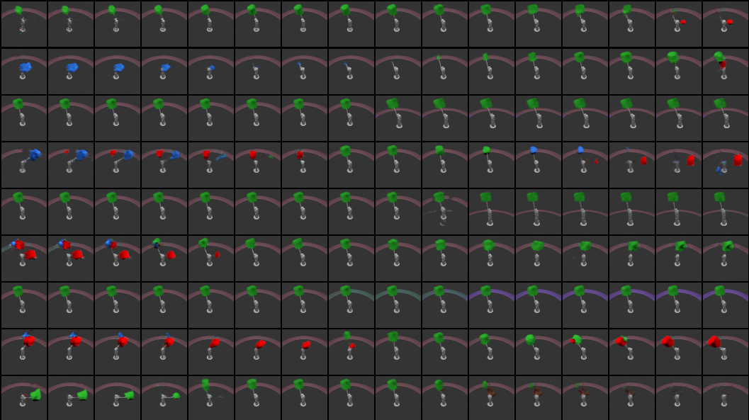
fig:beta-tcvae
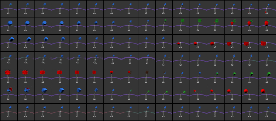
fig:beta-vae
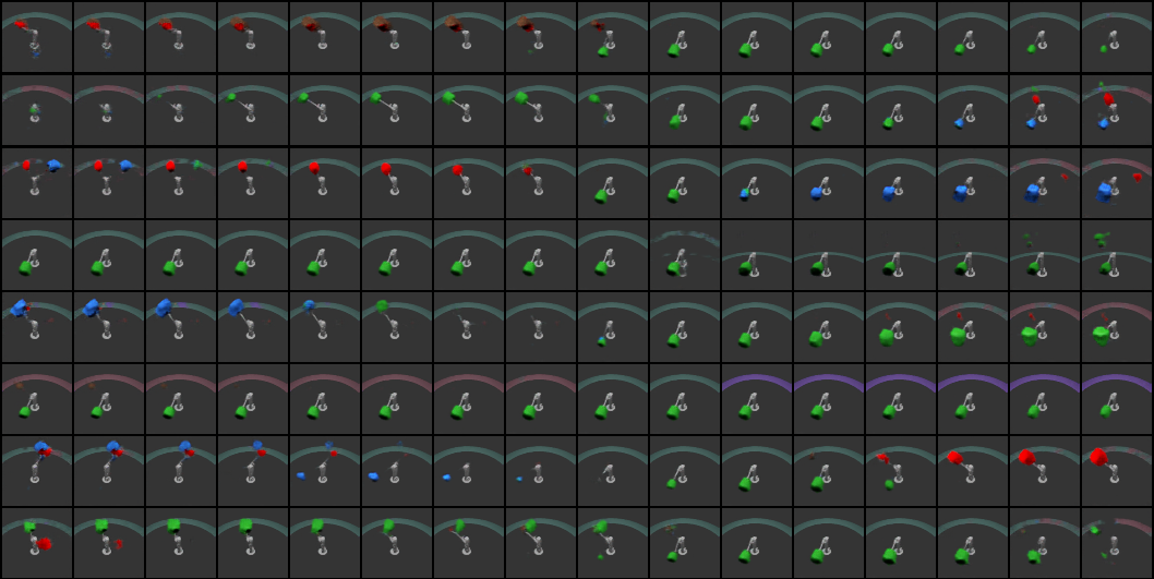
fig:factor-vae
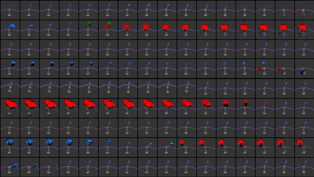
fig:dip-vae-i
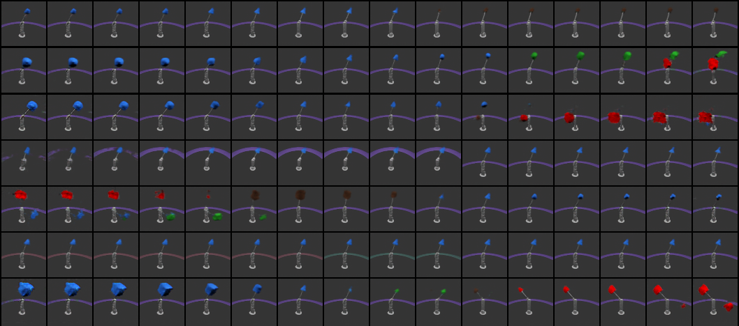
fig:dip-vae-ii
Appendix C Progression of Evaluation Metrics During Training
fig:subfigex1
fig:subfigex2