Measuring lensing ratios with future cosmological surveys

Abstract

The ratio between the CMB lensing/galaxy counts and the galaxy shear/galaxy counts cross-correlations combines the information from different cosmological probes to infer cosmographic measurements that are less dependent on astrophysical uncertainties and can constrain the geometry of the Universe. We discuss the future perspectives for the measurement of this lensing ratio as previously introduced, i.e. with the use of the Limber and flat-sky approximations and neglecting all the effects on the galaxy survey from observing on the past light cone. We then show how the cosmological information in this estimator is affected by the Limber approximation and by the inclusion of the redshift space distortions (RSD) and lensing magnification contributions to the galaxy number counts. We find that the lensing magnification contribution induces a multipole dependence of the lensing ratio that we show to be detectable at a statistical significant level combining post-$Planck$ CMB surveys and a Euclid-like experiment. We propose an improved estimator which takes into account this angular scale dependence. Using this extended formalism, we present forecasts for upcoming and future cosmological surveys, and we show at which extent the lensing ratio information can improve the CMB constraints on cosmological parameters. We get that for extended cosmological models where the neutrino mass, the spatial curvature and the dark energy equation of state are allowed to vary, the constraints from $Planck$ on these parameters and on $H_{0}$ can be reduced by $\sim 40\%$ with the inclusion of a single lensing ratio and by $\sim 60$-70% adding the joint measurement of 9 lensing ratios with a Euclid-like survey. We also find that neglecting the contribution from lensing magnification can induce a bias on the derived cosmological parameters in a combined analysis.

I Introduction

Weak gravitational lensing is one of the most direct probes of the distribution of dark matter and it is correlated with the intervening process of structure formation. Ratios between cross-correlations of galaxies and weak lensing at two different source planes in redshift have been proposed as cosmographic distance measurements Jain:2003tba ; Bernstein:2003es ; Zhang:2003ii ; Bernstein:2005en ; Hu:2007jh ; Das:2008am . The role of these ratio estimators between the weak lensing at two different redshift and a matter tracer as a cosmographic measure becomes extremely transparent under different approximations, such as the Limber and flat sky approximation, and the limit in which the foreground distribution is extremely peaked in redshift.

Being a ratio between two cross-correlation terms with the same lens, this estimator is largely independent on the clustering bias of the lens and weak lensing systematics, but depends on most of the background cosmological parameters. By taking one of the source planes as the CMB last scattering surface, the lever arm of such a lensing ratio estimator becomes somewhat maximal Hu:2007jh ; Das:2008am .

The scientific potential of the CMB lensing ratio as a cosmographic measurement for the next generation of CMB and LSS experiments has been forecast in several papers Das:2008am ; Ade:2018sbj ; Prat:2018yru . The estimator for the lensing ratio between CMB lensing/galaxies and galaxy shear/galaxies has already been applied to real data Miyatake:2016gdc ; Prat:2018yru . Miyatake et al. Miyatake:2016gdc used CMASS 1010.4915 and CFHTLens 1210.8156 for galaxy lenses and sources, respectively, and CMB lensing from $Planck$ 2015 1502.01591 . Prat et al. Prat:2018yru used galaxy position and lensing from DES Y1 1708.01530 and CMB lensing from a combination of $Planck$ 2015 and SPT 1705.00743 .

In this paper we study and extend the lensing ratio estimator as introduced by Das and Spergel in Das:2008am (henceforth DS) and we study its scientific capabilities in the context of future cosmological observations. We show how the approximations in the galaxy and lensing kernel and the finite width in redshift of the lenses density distributions affect to the multipole dependence of the lensing ratio. The inclusion of the lensing magnification contribution in the galaxy number counts introduces a further and larger dependence on the multipoles, which we show to be detected with future cosmological observations, and calls for an extension of a lensing ratio estimator which takes into account the dependence on multipoles.

Our paper is organized as follows. After this introduction, we introduce the notation for the CMB lensing/galaxy and galaxy shear/galaxy cross-correlation, respectively, in Section II. In Section III we introduce the experimental specifications of the CMB anisotropies and galaxy surveys we use in our forecasts. In Section IV we forecast the capabilities of a Euclid-like 1110.3193 experiment alone and in combination with galaxy lenses at lower redshift from DESI 1611.00036 and SPHEREx 1412.4872 in measuring the lensing ratio as originally introduced in DS. In Section V we consider the ratio between the CMB lensing/galaxy and galaxy shear/galaxy cross-correlations without approximations and replacing the galaxy density with the galaxy number counts including RSD and lensing magnification contributions and introduce its optimal estimator and minimum variance. In Section VI we forecast the expected errors on cosmological parameters by using the novel methodology introduced in Section V. In Section VII we draw our conclusions.

II Formalism

In this section we define the quantities involved in the angular power spectra of the cross-correlation between a foreground lens galaxy population and a background weak lensing source that comes from the CMB or from the galaxy shear. We define the angular power spectrum as

$$\delta_{\ell\ell^{\prime}}\delta_{mm^{\prime}}C_{\ell}^{a}=\langle a_{\ell m}a^{*}_{\ell^{\prime}m^{\prime}}\rangle$$ (1)

where $a_{\ell m}$ are the spherical harmonic coefficients obtained from the expansion of a scalar field with spin-0 spherical harmonics as

$$a\left(\hat{\bf n}\right)=\sum_{\ell m}a_{\ell m}Y^{*}_{\ell m}\left(\hat{\bf n}\right)\,.$$ (2)

We are interested in the cross-correlation of a foreground galaxy number density field with two different backgrounds as the convergence field from the weak lensing of galaxies and of the CMB. The angular power spectrum can be calculated as

$$C_{\ell}^{XY}=4\pi\int\frac{\mathrm{d}k}{k}{\cal P}(k)I^{X}_{\ell}(k)I^{Y}_{\ell}(k)$$ (3)

where ${\cal P}(k)\equiv k^{3}P(k)/(2\pi^{2})$ is the dimensionless primordial power spectrum and $I^{X}_{\ell}(k)$ is the kernel for the $X$ field for unit primordial power spectrum.

All the weak lensing quantities can be defined from the lensing potential

$$\phi\left(\hat{\bf n},\chi\right)=\frac{2}{c^{2}}\int_{0}^{\chi}\mathrm{d}\chi^{\prime}\frac{\chi-\chi^{\prime}}{\chi\chi^{\prime}}\Phi\left(\chi^{\prime}\hat{\bf n},\chi^{\prime}\right)$$ (4)

where $\Phi\left(\hat{\bf n},\chi\right)$ is the gravitational potential. The comoving distance is

$$\chi(z)=\int_{0}^{z}\frac{c\,\mathrm{d}z^{\prime}}{H(z^{\prime})}\,.$$ (5)

The observable 2-dimensional lensing potential, averaged over background sources with a redshift distribution $W_{b}\left(\chi\right)$, is given by

$$\phi\left(\hat{\bf n}\right)=\frac{2}{c^{2}}\int_{0}^{\chi}\frac{\mathrm{d}\chi^{\prime}}{\chi^{\prime}}q_{b}\left(\chi^{\prime}\right)\Phi\left(\chi^{\prime}\hat{\bf n},\chi^{\prime}\right)$$ (6)

where $q_{b}\left(\chi\right)$ is the lensing efficiency (for a given background distribution $W_{b}$) defined as

$$q_{b}\left(\chi\right)=\int_{\chi}\mathrm{d}\chi^{\prime}\frac{\chi^{\prime}-\chi}{\chi^{\prime}}W_{b}\left(\chi^{\prime}\right)\,.$$ (7)

By expanding the gravitational potential in Fourier space and using the plane-wave expansion, we can define the lensing potential kernel as Jain:1996st

$$I^{\phi}_{\ell}(k)=2\left(\frac{3\Omega_{m}H_{0}^{2}}{2k^{2}c^{2}}\right)\int\frac{\mathrm{d}\chi}{(2\pi)^{3/2}}\frac{q_{b}\left(\chi\right)}{\chi a(\chi)}j_{\ell}\left(k\chi\right)\delta\left(k,\chi\right)\,,$$ (8)

where $\Omega_{m}$ is the present-day matter density, $H_{0}$ is the Hubble constant, $\delta(k,\chi)$ is the comoving-gauge matter density perturbation, and $j_{\ell}$ the spherical Bessel functions. In case of CMB lensing, the source distribution can be approximated by $W_{\rm CMB}\left(\chi\right)\simeq\delta_{\rm D}\left(\chi-\chi_{*}\right)$ and the lensing efficiency by

$$q_{\rm CMB}\left(\chi\right)\simeq\frac{\chi_{*}-\chi}{\chi_{*}}$$ (9)

where $\chi_{*}$ is the comoving distance at the surface of last scattering, and Eq. (8) reduces to

$$I^{\phi_{\rm CMB}}_{\ell}(k)=2\left(\frac{3\Omega_{m}H_{0}^{2}}{2k^{2}c^{2}}\right)\\ \times\int\frac{\mathrm{d}\chi}{(2\pi)^{3/2}}\frac{\chi_{*}-\chi}{\chi_{*}\chi}\frac{1}{a(\chi)}j_{\ell}\left(k\chi\right)\delta\left(k,\chi\right)\,.$$ (10)

Finally the convergence $\kappa=\nabla^{2}\phi/2$ can be expanded in spherical-harmonics as

$$\kappa\left({\bf\hat{n}}\right)=-\frac{1}{2}\sum_{\ell,m}\ell(\ell+1)\phi_{\ell m}Y_{\ell}^{m}\left({\bf\hat{n}}\right)$$ (11)

and we can relate the two kernel functions by

$$I_{\ell}^{\kappa}(k)=\frac{\ell(\ell+1)}{2}I_{\ell}^{\phi}(k)\,.$$ (12)

The 2-dimensional integrate window function for the galaxy number counts is

$$I^{G}_{\ell}(k)=\int\frac{\mathrm{d}\chi}{(2\pi)^{3/2}}W_{f}(\chi)\Delta^{s}_{\ell}(k,\chi)$$ (13)

where $\Delta^{s}_{\ell}(k,\chi)$ is the synchronous gauge source counts Fourier transformed and expanded into multipoles and $W_{f}(\chi)$ is the foreground redshift distribution of galaxies. We assume that $\Delta^{s}_{\ell}(k,\chi)$ is related to the underlying matter density field through a redshift dependent galaxy bias $b_{g}$ as $\Delta^{s}_{\ell}(k,\chi)=b_{g}(\chi)\delta(k,\chi)j_{\ell}\left(k\chi\right)$.

Finally, we define the lensing ratio as DS

$$r_{\ell}\equiv\frac{C_{\ell}^{\kappa_{\rm CMB}G}}{C_{\ell}^{\kappa_{\rm gal}G}}\,.$$ (14)

III Data and specifications

We define here the specifications for the future large scale structure and CMB surveys considered in order to produce the mock signal and noise data. The lensing ratio estimator is based in the cross-correlations between three ingredients: a tracer for the foreground galaxy population, a background of source galaxies traced by a Euclid-like photometric survey; and the CMB lensing background source, for which we consider a $Planck$-like experiment and many future experiments.

We create the mock data for the angular power spectra using CLASSgal Blas:2011rf ; 1307.1459 . The non-linear corrections are modeled as halofit with the recipe by 1208.2701 . For the fiducial cosmology we assume a $\Lambda$CDM+$\sum m_{\nu}$ model with one massive neutrino consistent with the $Planck$ 2018 results 1807.06209 . We use $\Omega_{b}h^{2}$ = 0.022383, $\Omega_{c}h^{2}$ = 0.12011, $H_{0}$ = 67.32 km s^-1 Mpc^-1, $\tau$ = 0.0543, $n_{s}$ = 0.96605, $\ln(10^{10}A_{s})$ = 3.0448 and $\sum m_{\nu}$ = 0.06 eV.

III.1 Galaxy lenses

For the foreground lens population we use a Euclid-like spectroscopic survey and lower redshift populations like DESI and SPHEREx that allow to increase the background number of objects and the distance between the lens and the sources, which come from the Euclid photometric survey. We describe here the specifications of these experiments.

We adopt as baseline for a given lens population narrow slices with $\Delta z$ = 0.1. For this, we convolve the number density distribution ${\rm d}N/{\rm d}z$ with a Gaussian probability distribution for the measured redshift given the redshift accuracy. Following Ma:2005rc , the number density distribution of a single bin is expressed as

$$\frac{{\rm d}n_{\rm gal}^{i}}{{\rm d}z}=\frac{{\rm d}N}{{\rm d}z}\int_{z_{\rm min}}^{z_{\rm max}}{\rm d}z_{m}p(z_{m}|z)\,,$$ (15)

where $z_{\rm min}$, $z_{\rm max}$ are the edges of the redshift bin and $p(z_{m}|z)$ is the probability density for the measured redshift $z_{m}$ given the true redshift $z$ of the galaxy, given by

$$p(z_{m}|z)=\frac{1}{\sqrt{2\pi}\sigma_{z}}e^{-\frac{1}{2}(z_{m}-z)^{2}/\sigma_{z}^{2}}\,.$$ (16)

Inserting Eq. (16) into Eq. (15) we obtain:

$$\frac{{\rm d}n_{i}}{{\rm d}z}=\frac{1}{2}\frac{{\rm d}N}{{\rm d}z}\left[{\rm erf}\left(\frac{z_{\rm max}-z}{\sqrt{2}\sigma_{z}}\right)-{\rm erf}\left(\frac{z_{\rm min}-z}{\sqrt{2}\sigma_{z}}\right)\right]$$ (17)

where erf is the error function.

In the harmonic space, the Poisson shot noise for a given foreground population at redshift $z_{i}$ is obtained as the inverse of the number of objects per steradian,

$${\cal N}_{\ell}^{G}(z_{i})=\frac{4\pi f_{\rm sky}}{\bar{n}_{\rm g}^{i}}$$ (18)

where $f_{\rm sky}$ is the sky fraction and ${n_{\rm g}^{i}}$ is the total number of galaxies.

III.1.1 Euclid-like spectroscopic survey

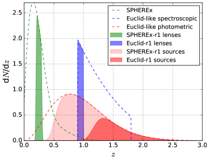
The Euclid spectroscopic survey will measure the galaxy clustering from millions of $H\alpha$ emitters in a redshift range $0.9\leq z\leq 1.8$ with a sky coverage of 15000 deg². The number density distribution ${\rm d}N/{\rm d}z$ of the survey is fitted from the model 3 data by Pozzetti:2016cch using a flux threshold $F_{\textup{H}\alpha}>2\times 10^{-16}\ \text{erg}\ \text{cm}^{-2}\ \text{s}^{-1}$. This yields as total number density of objects $\bar{n}_{\mathrm{g}}=2039$ sources per deg², for which we introduce a 50% factor due to the Euclid completeness and purity. We assume a bias evolution function $b_{g}(z)=0.7+0.7z$ according to the fitting for H$\alpha$ emission line object from 1903.02030 . The redshift accuracy is characterized by a dispersion $\sigma_{z}=0.001(1+z)$. We represent in Fig. 1 the ${\rm d}N/{\rm d}z$ of the full survey and the selected foreground population for the first redshift bin at 0.9 $<z_{\rm lens}<$ 1. We will refer hereafter this foreground configuration as Euclid-r1.

III.1.2 Lenses at lower redshift

For the foreground lens populations at lower redshift we consider the ground-based survey Dark Energy Spectroscopic Instrument (DESI) and the recently approved NASA mission Spectro-Photometer for the History of the Universe, Epoch of Reionization, and Ices Explorer (SPHEREx).

DESI is an ongoing spectroscopic survey that covers $\sim 14000$ deg² in the sky. Here we consider the lower redshift target objects: the Bright Galaxy Sample (BGS), which will measure $\sim 10$ million galaxies at 0 $<z<$ 0.4. We adopt the specifications in 1611.00036 for the number density distribution and the bias redshift evolution, which is given by $b_{g}(z)=1.34/D(z)$. The redshift accuracy is given by $\sigma_{z}=0.001(1+z)$. The overlapping sky fraction with Euclid will be limited to $\sim 4000$ deg².

SPHEREx will be a full-sky spectro-photometric survey that can operate with different configurations depending on the number of objects and redshift accuracy. In this work we assume SPHEREx-2, a configuration with $\sigma_{z}=0.008(1+z)$ and $\sim 70$ million objects. Since this survey will cover $\sim 80\%$ of the sky, there will be full overlap with the background from Euclid and all the CMB experiments. We represent in Fig. 1 the ${\rm d}N/{\rm d}z$ of the full survey and the lens foreground population for a bin at 0.2 $<z_{\rm lens}<$ 0.3. We will refer hereafter this foreground configuration as SPHEREx-r1.

III.2 Galaxy shear sources: Euclid-like photometric survey

The Euclid photometric survey will measure both galaxy clustering and weak lensing from a sample of billions of galaxies. Here we will consider the weak lensing from a given background population. We parametrize the ${\rm d}N/{\rm d}z$ of the survey as

$$\frac{{\rm d}N}{{\rm d}z}\propto z^{\alpha}\exp\left[-\left(\frac{z}{z_{0}}\right)^{\beta}\right]$$ (19)

where $\alpha$ = 2, $\beta$ = 3/2, $z_{0}=z_{\rm mean}/\sqrt[]{2}$ and $z_{\rm mean}$ = 0.9 is the mean redshift of the survey. The number density of the sources population is $\bar{n}_{\mathrm{g}}=30$ objects per arcmin². The sky coverage is 15000 deg² as well as for the spectroscopic survey, and the bias is assumed to evolve with redshift following $b_{G}(z)=\sqrt{1+z}$ 1206.1225 .

We assume that the background population is given by a broad bin that maximizes the number of objects behind the lenses without overlapping with them. For this, we convolve the ${\rm d}N/{\rm d}z$ of the photometric survey with a Gaussian redshift probability distribution with a dispersion $\sigma_{z}=0.05(1+z)$, following Eq. (17). We show in Fig. 1 the ${\rm d}N/{\rm d}z$ of the photometric survey and the maximal background source populations for the two foregrounds of the Euclid-r1 and SPHEREx-r1 configurations.

The shear noise for the background population for a redshift bin at $z_{i}$ is obtained as

$${\cal N}_{\ell}^{\kappa_{\rm gal}}(z_{i})=\sigma_{\epsilon}^{2}\frac{4\pi f_{\rm sky}}{\bar{n}_{\rm g}^{i}}$$ (20)

where $\sigma_{\epsilon}$ is the intrinsic ellipticity RMS, for which we adopt $\sigma_{\epsilon}$ = 0.22, $f_{\rm sky}$ is the sky coverage and ${n_{\rm g}^{i}}$ is the number of sources.

Figure 1: Survey configuration for the lensing ratio. The green dashed curve represents the normalized ${\rm d}N/{\rm d}z$ of SPHEREx and the green shaded area corresponds to a bin at 0.2 $<z<$ 0.3 for the foreground population of the SPHEREx-r1 configuration. The blue dashed curve represents the normalized ${\rm d}N/{\rm d}z$ of the Euclid-like spectroscopic survey, and the blue shaded area corresponds to the bin at 0.9 $<z<$ 1.0 that traces the foreground of the Euclid-r1 configuration. The red dashed curve represents the normalized ${\rm d}N/{\rm d}z$ of the Euclid-like photometric survey, and the pink and red shaded areas correspond to the background of source galaxies beyond the SPHEREx-r1 and Euclid-r1 lenses.

III.3 CMB lensing source

For the CMB lensing background source we consider as surveys the ESA mission $Planck$ 1807.06205 , the ground-based future experiments Simons Observatory (SO) 1808.07445 and CMB Stage-4 (S4) 1610.02743 , the proposed space missions Lite satellite for the studies of B-mode polarization and Inflation from cosmic background Radiation Detection (LiteBIRD) Matsumura:2016sri , and the two concepts Probe of Inflation and Cosmic Origins (PICO) 1902.10541 and Polarized Radiation Imaging and Spectroscopy Mission (PRISM) 1909.01591 . The specifications of these experiments will be also used for temperature and polarization for a quantitative assessment of what the lensing ratio can add to the information of the CMB fields alone.

We reconstruct the minimum variance (MV) estimator for the CMB lensing noise ${\cal N}_{\ell}^{\phi\phi}$ using the temperature and polarization noise ${\cal N}_{\ell}^{TT}$ and ${\cal N}_{\ell}^{EE}$. This is done combining the $TT$, $EE$, $BB$, $TE$, $TB$, $EB$ estimators following the Hu-Okamoto algorithm astro-ph/0301031 and using the public code quicklens. For the $TT$ and $EE$ channels we calculate the isotropic noise deconvolved with the instrument beam using the formula

$${\cal N}_{\ell}^{X}=w_{X}^{-1}b_{\ell}^{-2},\qquad b_{\ell}=e^{-\ell(\ell+1)\theta_{\rm FWHM}^{2}/16\ln 2}$$ (21)

where $\theta_{\rm FWHM}$ is the FWHM of the beam in radians and $w_{TT}$, $w_{EE}$ are the inverse square of the detector noise level for temperature and polarization in arcmin^-1 $\mu$K^-1.

In order to provide specifications of simulated $Planck$-like data leading to uncertainties on the cosmological parameters compatible with the latest results in 1807.06209 we adopt $w_{TT}$ = 33 $\mu$K arcmin, $w_{EE}$ = 70.2 $\mu$K arcmin and $\theta_{\rm FWHM}=7.3$ arcmin for the 143 GHz channel and assume a sky fraction of $f_{\rm sky}=0.7$. We re-adapt the noise in polarization ${\cal N}_{\ell}^{EE}$ inflating the noise in polarization at $\ell<30$ in order to obtain estimates for the uncertainty in the optical depth compatible with the $Planck$ 2018 results. For the $Planck$-like survey, the effective noise bias for the CMB lensing power spectrum is obtained from the inverse weighted sum of the specifications of the 143 and 217 GHz channels in Adam:2015rua to match the $Planck$ 2018 performances 1807.06209 . We assume a sky coverage $f_{\rm sky}$ = 0.7 also for the lensing, which fully overlap with Euclid and we set $\ell_{\rm max}$ = 1500.

For SO we adopt the specifications of the six frequency bands listed in 1808.07445 . We assume $f_{\rm sky}$ = 0.4 and $\ell_{\rm max}$ = 3000. Since this is a ground-based experiment, the largest scales will not be seen by SO, hence we set $\ell_{\rm min}=30$ and consider the $Planck$ specifications for $2\leq\ell\leq 29$ (hereafter we call $Planck$+SO to this combination). We rescale the MV noise bias for the CMB lensing to match the baseline configuration in 1808.07445 . Given that the experiment will be based in the southern hemisphere, there will not be full overlap with the Euclid sky coverage. We assume that the common sky fraction will be around 25% of the sky.

For S4 we adopt $w_{TT}$ = 1 $\mu$K arcmin, $w_{EE}=\sqrt{2}$ $\mu$K arcmin, $\theta_{\rm FWHM}=3$ arcmin 1610.02743 and we assume as for SO $f_{\rm sky}$ = 0.4 and $\ell_{\rm max}$ = 3000. Since this experiment will be also based in the southern hemisphere, we limit as well the overlapping sky fraction with Euclid to 25% and adopt the $Planck$ noise for $\ell<$ 30.

For LiteBird we combine the 7 channels described in 1612.08270 . We assume 70% sky fraction and since this mission will be optimized for large scales, we adopt $\ell_{\rm max}$ = 1350.

For PICO we use the 7 channels ranging from 75 to 220 GHz given in 1902.10541 . We assume $\ell_{\rm max}$ = 3000 and 70% of sky coverage.

For PRISM we sum the 12 channels ranging from 52 to 385 GHz in 1909.01591 . We adopt $\ell_{\rm max}$ = 4000 and 75% for the sky fraction.

Figure 2: Signal of the CMB lensing potential data and its noise computed for the experiments considered using the minimum variance estimator.

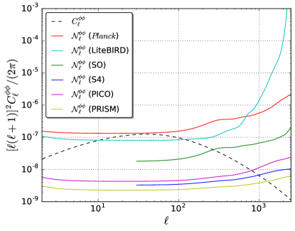
We show in Fig. 2 the CMB lensing potential noise ${\cal N}_{\ell}^{\phi\phi}$ obtained for the experiments described above.

IV Cosmographic lensing ratio measurements

In this section we study how under some approximations the lensing ratio $r_{\ell}$ can be interpreted as a cosmographic measurement that does not depend on the multipoles, astrophysical uncertainties and perturbations. We then present forecasts for the error on the lensing ratio for this previously introduced limit using the future cosmological surveys mock data described in Section III and explore how this uncertainty varies with the foreground population redshift $z_{\rm lens}$ and the selected background.

IV.1 The cosmographic ratio limit

We show here the limit in which the lensing ratio $r_{\ell}$ defined in Section II becomes a geometrical quantity independent of the angular scale, the power spectrum and the galaxy bias. This limit needs to assume the Limber approximation, to select a foreground lens population which is narrow enough in redshift and to neglect the effects on the galaxy number counts from observing on the past light cone.

IV.1.1 Limber approximation

In order to speed up the computation of Eq. (3), which is time-consuming due to the rapid oscillations of the spherical Bessel function at high multipoles, it is commonly adopted the Limber approximation Limber:1954zz which is accurate at high-$\ell$. It consists in replacing the spherical Bessel function $j_{\ell}(k\chi)$ with a Dirac delta-function $\delta_{\rm D}$

$$j_{\ell}(k\chi)\to\sqrt{\frac{\pi}{2(\ell+1/2)}}\delta_{\rm D}\left(\ell+\frac{1}{2}-k\chi\right)\,.$$ (22)

We can then approximate the kernel functions (8)-(10)-(13) obtaining the following angular power spectra

$$C_{\ell}^{\phi\phi}(z_{i},z_{j})=\frac{4}{(\ell+1/2)^{4}}\left(\frac{3\Omega_{\rm m}H_{0}^{2}}{2c^{2}}\right)^{2}\\ \times\int\mathrm{d}\chi\frac{q_{b_{i}}(\chi)q_{b_{j}}(\chi)}{a^{2}(\chi)}P_{\delta}\left(\frac{\ell+1/2}{\chi},\chi\right)\,,$$ (23)

$$C_{\ell}^{GG}(z_{i},z_{j})=\\ \int\mathrm{d}\chi\frac{W_{f_{i}}(\chi)W_{f_{j}}(\chi)}{\chi^{2}}b_{g}^{2}(\chi)P_{\delta}\left(\frac{\ell+1/2}{\chi},\chi\right)\,,$$ (24)

$$C_{\ell}^{\phi G}(z_{i},z_{j})=\frac{2}{(\ell+1/2)^{2}}\left(\frac{3\Omega_{\rm m}H_{0}^{2}}{2c^{2}}\right)\\ \times\int\mathrm{d}\chi\frac{q_{b_{i}}(\chi)W_{f_{j}}(\chi)}{a(\chi)\chi}b_{g}(\chi)P_{\delta}\left(\frac{\ell+1/2}{\chi},\chi\right)\,,$$ (25)

for background sources, foreground lenses, and their cross-correlation, where the matter power spectrum is defined as

$$\langle\delta({\bf k},\chi)\delta^{*}({\bf k^{\prime}},\chi)\rangle=(2\pi)^{3}P_{\delta}(k,\chi)\delta_{\rm D}({\bf k}-{\bf k^{\prime}})\,.$$ (26)

Figure 3: Impact of the Limber approximation on both lensing-galaxy cross-correlation angular power spectra (left panel) and on the lensing ratio (right panel), using the Euclid-r1 configuration at $z_{\rm lens}$ = 0.95

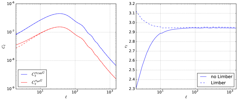
We show in Fig. 3 the effect of the Limber approximation in the cross-correlation angular power spectra $C_{\ell}^{\kappa_{\rm CMB}G}$ and $C_{\ell}^{\kappa_{\rm gal}G}$ and in the lensing ratio $r_{\ell}$, using the Euclid-r1 configuration. We find that the Limber approximation changes the signal of the denominator $C_{\ell}^{\kappa_{\rm gal}G}$ and hence the ratio $r_{\ell}$ at the lowest multipoles, smoothing the $\ell$-dependence that appears when this approximation is not used.

In DS it is also considered the flat-sky approximation. In this limit, the sky is approximated by a 2-dimensional plane tangential to the celestial sphere and mathematically expansions in spherical harmonics are replaced by Fourier expansions

$$\sum_{\ell,m}\phi_{\ell,m}Y_{\ell}^{m}(\hat{\bf n})\to\int\frac{\mathrm{d}^{2}{\boldsymbol{\theta}}}{(2\pi)^{2}}\phi({\bf\ell})e^{\imath{\boldsymbol{\theta}}\cdot\hat{\bf n}}\,.$$ (27)

The relation between the convergence and lensing kernel (12) is then

$$I_{\ell}^{\kappa}(k)\simeq\frac{\ell^{2}}{2}I_{\ell}^{\phi}(k)\,.$$ (28)

The flat-sky approximation does not affect the ratio since the difference in the prefactor $\ell+1/2\to\ell$ cancels out.

IV.1.2 Narrow foreground

If the redshift distribution of the foreground population is narrow enough in redshift or if we have a redshift accuracy $\sigma_{z}$ sufficient to slice the foreground population in narrow redshift bins, we can approximate the foreground redshift distribution as a Dirac delta-function

$$W_{f}(\chi)\propto\delta_{\rm D}(\chi-\chi_{f})\,,$$ (29)

where $\chi_{f}$ is the peak of the distribution. We then find

$$C_{\ell}^{\phi G}(z_{f},z_{b})=\frac{2}{(\ell+1/2)^{2}}\left(\frac{3\Omega_{\rm m}H_{0}^{2}}{2c^{2}}\right)\\ \times\frac{b(\chi_{f})P_{\delta}\left(\frac{\ell+1/2}{\chi_{f}},\chi_{f}\right)}{a(\chi_{f})\chi_{f}}\int\mathrm{d}\chi\frac{\chi-\chi_{f}}{\chi}W_{b}(\chi)\,.$$ (30)

Under these approximations the ratio loses the $\ell$-dependence, we obtain a quantity which depends only on background parameters ($H_{0}$, $\Omega_{X}$, $w_{0}$, …), and the clustering bias cancels out, i.e.

$$r=\frac{\chi_{*}-\chi_{f}}{\chi_{*}}\frac{1}{\int\mathrm{d}\chi\frac{\chi-\chi_{f}}{\chi}W_{b}({\chi})}\,.$$ (31)

Finally, if also the background distribution is sufficiently thin we can recover the standard cosmographic expression for the ratio

$$r=\frac{\chi_{*}-\chi_{f}}{\chi_{b}-\chi_{f}}\frac{\chi_{b}}{\chi_{*}}\,,$$ (32)

where we assumed $W_{b}(\chi)\propto\delta_{\rm D}(\chi-\chi_{b})$.

IV.2 Forecasts for future experiments

We quantify the accuracy that will be reachable on the lensing ratio measurement for future experiments in the limit in which it can be considered as an $\ell$-independent quantity ($r_{\ell}\simeq r$). For this, we follow the formalism by DS in order to compute the error on $r$.

The log-likelihood is defined as

$$\chi^{2}(r)=\sum_{\ell}\frac{Z_{\ell}^{2}}{\sigma^{2}(Z_{\ell})}$$ (33)

where $Z_{\ell}=C_{\ell}^{\kappa_{\rm CMB}G}-rC_{\ell}^{\kappa_{\rm gal}G}$. For the variance of $Z_{l}$ at a fiducial value of the ratio $r_{0}$, we use the extended definition by Prat:2018yru , which accounts for partial overlap in the sky between surveys,

$$\sigma^{2}(Z_{\ell})=\frac{1}{(2\ell+1)}\\ \times\bigg{[}\frac{1}{f_{\rm sky}^{\kappa_{\rm CMB}G}}\Big{(}\bar{C}_{\ell}^{\kappa_{\rm CMB}\kappa_{\rm CMB}}\bar{C}_{\ell}^{GG}+(C_{\ell}^{\kappa_{\rm CMB}G})^{2}\Big{)}\\ +\frac{r_{0}^{2}}{f_{\rm sky}^{\kappa_{\rm gal}G}}\Big{(}\bar{C}_{\ell}^{\kappa_{\rm gal}\kappa_{\rm gal}}\bar{C}_{\ell}^{GG}+(C_{\ell}^{\kappa_{\rm gal}G})^{2}\Big{)}\\ -2r_{0}\frac{f_{\rm sky}^{\kappa_{\rm CMB}\kappa_{\rm gal}G}}{f_{\rm sky}^{\kappa_{\rm CMB}G}f_{\rm sky}^{\kappa_{\rm gal}G}}\Big{(}C_{\ell}^{\kappa_{\rm CMB}\kappa_{\rm gal}}\bar{C}_{\ell}^{GG}+C_{\ell}^{\kappa_{\rm CMB}G}C_{\ell}^{\kappa_{\rm gal}G}\Big{)}\bigg{]}$$ (34)

where $\bar{C}_{\ell}^{XX}=C_{\ell}^{XX}+{\cal N}_{\ell}^{XX}$ includes the signal and noise power spectra, and the $f_{\rm sky}$ factors account for the overlapping sky fraction between each pair of probes. We introduce the maximum likelihood estimator for the lensing ratio solving $\partial\chi^{2}/\partial r=0$ as DS

$$\hat{r}=\frac{\sum_{\ell}C_{\ell}^{\kappa_{\rm CMB}G}C_{\ell}^{\kappa_{\rm gal}G}/\sigma^{2}(Z_{\ell})}{\sum_{\ell}(C_{\ell}^{\kappa_{\rm gal}G})^{2}/\sigma^{2}(Z_{\ell})}\,,$$ (35)

and we then compute the error on $\hat{r}$ as

$$\frac{1}{\sigma^{2}(\hat{r})}=\frac{1}{2}\frac{\partial^{2}\chi^{2}(r)}{\partial r^{2}}=\sum_{\ell}\frac{(C_{\ell}^{\kappa_{\rm gal}G})^{2}}{\sigma^{2}(Z_{\ell})}\,.$$ (36)

In Fig. 4 we represent $\hat{r}$ and its error as a function of $z_{\rm lens}$ for the 9 possible bins of the Euclid-like spectroscopic survey and three of the CMB experiments considered: $Planck$, $Planck$+SO and PRISM. As suggested in Das:2008am ; Prat:2018yru , this estimator is specially sensitive to the curvature of the Universe and the equation of state of dark energy. We therefore calculate also $\hat{r}$ for cosmologies beyond $\Lambda$CDM shifting $w_{0}$ and $\Omega_{k}$ by a given amount.

Figure 4: Forecast measurements of the maximum likelihood estimator for the lensing ratio $\hat{r}$ (35) with their errors as a function of the Euclid-like spectroscopic foreground redshift $z_{\rm lens}$ for three CMB experiments: $Planck$, $Planck$+SO and PRISM. The central dots and errorbars correspond to a $\Lambda$CDM cosmology while the red and blue dashed curves represent the values of $\hat{r}$ obtained shifting by a certain amount $\Omega_{k}$ and $w_{0}$, respectively.

Figure 5: As for Fig. 4 but using $Planck$ as CMB lensing background with a variable galaxy background beyond each foreground (blue errorbars) and a fixed galaxy background at 2.0 $<z<$ 2.5 (red errorbars).

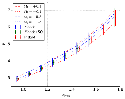
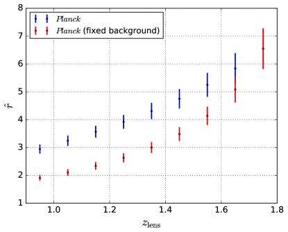
We find that for post-$Planck$ CMB experiments in which the CMB lensing noise will be reduced by a significant amount, the ratio will be measured with better accuracy specially for the lower redshift bins. At higher redshift for the lenses $z_{\rm lens}$, the higher noise of the galaxy surveys gives less precise measurements. For the non-standard cosmologies, we find that $\hat{r}$ is sensitive in particular to the curvature variations.

For the Euclid-like spectroscopic lenses and using the $Planck$ CMB lensing, the best measurement will be $\sigma(\hat{r})/\hat{r}$ = 5.5%, corresponding to the Euclid-r1 configuration at 0.9 $<z_{\rm lens}<$ 1.0. If we take a lower redshift lens at 0.2 $<z_{\rm lens}<$ 0.3 for DESI and SPHEREx, we get as relative errors 6.7% and 4.3%, respectively. This means that the measurement for DESI will be affected by the small overlapping sky fraction with Euclid, while using SPHEREx as foreground population can relatively improve the lensing ratio measurement. Using post-$Planck$ CMB lensing, we get as relative errors 3.2% and 2.3% for SO in combination with the Euclid-r1 and SPHEREx-r1 configurations, respectively. With PRISM, these two measurements improve to 1.4% and 0.7%, respectively.

In Fig. 5 we explore the effect of fixing the background galaxy shear sources to the Euclid-like photometric population placed behind the Euclid-like spectroscopic survey (i.e. behind the higher redshift lens on Fig. 4). The increase on the distances between the galaxy lens and source planes shifts the maximum likelihood ratio to lower values and also decreases the absolute error, but we find a very similar relative error in comparison with the variable background case. This also shows that the measurement is not limited by the background noise.

V A generalized lensing ratio estimator

In this section we show how the inclusion of the RSD and lensing magnification contributions to the galaxy number counts has an impact on the angular scale dependence of the lensing ratio $r_{\ell}$ and the cosmological information contained on it. We propose the introduction of a multipole dependent estimator to upgrade the formalism by DS and consider a more general case beyond assuming that $r$ is constant. We define the signal-to-noise ratio of the $\hat{r}_{\ell}$ estimator and evaluate the impact of including on the calculation the contributions beyond the density term.

V.1 Number counts angular power spectrum

Eq. (13) assumes only the contribution from the synchronous-gauge galaxy overdensity to the galaxy number counts. Here we quantify the relevance of including other terms to $\Delta^{s}_{\ell}(k,\chi)$ given by RSD and lensing magnification (see Challinor:2011bk ; Ballardini:2018cho for details). The RSD term is given by

$$\Delta^{\rm RSD}_{\ell}(k,\chi)=\frac{kv_{k}}{\cal H}j_{\ell}^{\prime\prime}(k\chi)$$ (37)

where $v_{k}$ is the velocity of the sources and ${\cal H}$ is the Hubble parameter. The lensing convergence contribution is given by

$$\Delta^{\rm lensing}_{\ell}(k,\chi)=\frac{\ell(\ell+1)}{2}(2-5s)\\ \times\int_{0}^{\chi}{\rm d}\chi^{\prime}\frac{\chi-\chi^{\prime}}{\chi\chi^{\prime}}\left[\phi_{k}(\chi^{\prime})+\psi_{k}(\chi^{\prime})\right]j_{\ell}(k\chi^{\prime})$$ (38)

where $\phi_{k}$ and $\psi_{k}$ are the metric perturbations in the longitudinal gauge and $s$ is the magnification bias, which accounts for the fact that observed galaxies are magnified by lensing. In this paper, we consider lensing magnification as the only observational effect on number counts with the density and RSD. We neglect the Doppler, Sachs-Wolfe and other integrated effects (ISW and time-delay) because they are negligible in the calculation of the ratio.

We derive and fit the functional form of the redshift dependence of the magnification bias $s(z)$ of the Euclid-like spectroscopic survey using the model 3 luminosity function by Pozzetti:2016cch . For a flux threshold of $F_{\rm cut}=2\times 10^{-16}$ erg s^-1 cm^-2 we find:

$$s(z)=0.33+0.46z+0.15z^{2}-0.16z^{3}+0.03z^{4}$$ (39)

Note that this fit is valid only for $z\geq 0.6$ since the model 3 by Pozzetti:2016cch does not include data for low redshift objects.

Figure 6: Impact of the RSD and lensing contributions on the lensing-galaxy cross-correlation angular power spectra (left panel) and on the lensing ratio estimator (right panel) for the Euclid-r1 configuration.

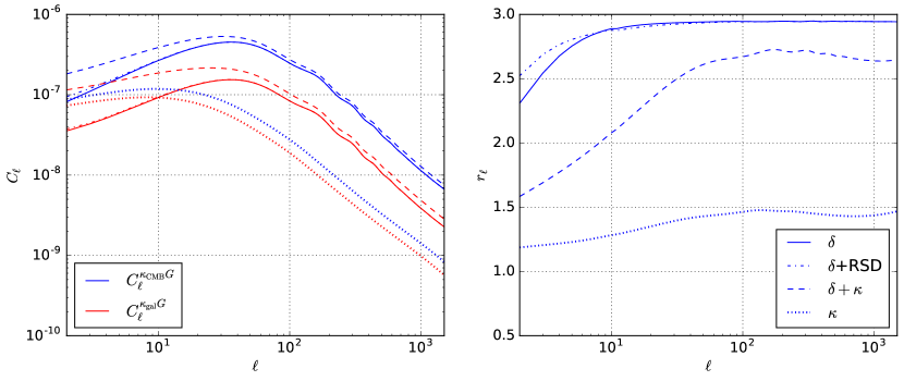
In Fig. 6 we show the impact of including the RSD term alone and both RSD and lensing contributions together in the cross-correlation angular power spectra $C_{\ell}^{\kappa_{\rm CMB}G}$ and $C_{\ell}^{\kappa_{\rm gal}G}$ and in the lensing ratio $r_{\ell}$, adopting the Euclid-r1 configuration.

For the case including only RSD, we find a small correction on the angular power spectra at low multipoles, which results in a slightly higher lensing ratio at $\ell<10$. When we consider also the lensing magnification, we obtain a larger positive contribution to both $C_{\ell}^{\kappa_{\rm CMB}G}$ and $C_{\ell}^{\kappa_{\rm gal}G}$ that is especially strong at large scales but holds also at higher multipoles. This results in a negative $\sim 10\%$ shift for $r_{\ell}$ given that the impact of including GR in the denominator $C_{\ell}^{\kappa_{\rm gal}G}$ is higher. The shape of the lensing ratio becomes less constant with $\ell$ once the lensing magnification contribution is considered.

We show here how the lensing term induces the $\ell$-dependence of the lensing ratio. If we consider the density term and the lensing contribution the kernel of the galaxy number counts becomes

$$I^{G}_{\ell}(k)\equiv I^{G_{1}}_{\ell}(k)+I^{G_{2}}_{\ell}(k)\\ =\int\frac{\mathrm{d}\chi}{(2\pi)^{3/2}}W_{f}(\chi)\left[\Delta^{s}_{\ell}(k,\chi)+\Delta^{\rm lensing}_{\ell}(k,\chi)\right]\,.$$ (40)

Using the Limber approximation, the first term of the lensing-galaxy cross-correlation is given by Eq. (25), and for the second term we find:

$$C_{\ell}^{\phi G_{2}}(z_{i},z_{j})=\frac{\ell(\ell+1)}{(\ell+1/2)^{2}}\left(\frac{3\Omega_{\rm m}H_{0}^{2}}{2c^{2}}\right)\\ \times\int\frac{\mathrm{d}\chi}{(2\pi)^{3}}\frac{q_{b_{i}}(\chi)}{a(\chi)\chi}\delta\left(\frac{\ell+1/2}{\chi},\chi\right)\left(\phi+\psi\right)\\ \times\int_{0}^{\chi}\mathrm{d}\chi^{\prime}\frac{\chi^{\prime}-\chi}{\chi^{\prime}\chi}(2-5s)W_{f_{j}}(\chi^{\prime})\,.$$ (41)

We note that in this case, the assumption of a narrow foreground would not eliminate the $\ell$-dependence of the ratio since the last integral is bound to $\chi$ and can not be simplified. We represent in Fig. 6 the contribution to the angular power spectra from the lensing magnification term ($\kappa$) and their ratio, showing that is not anymore an $\ell$-independent quantity. Nonetheless, the $\ell$-dependence can be alleviated using a different tracer for the galaxy foreground population which is not affected by the lensing magnification contribution as in Pourtsidou:2015qaa , where they used as a foreground the SKA HI intensity mapping survey.

V.2 Signal-to-noise analysis

We extend here the formalism to compute the error on the lensing ratio by DS to consider the angular scale dependence of the ratio. We introduce the signal-to-noise ratio (SNR) of an $\ell$-dependent estimator $\hat{r}_{\ell}$ and compare its value to the ratio studied before.

We start by assuming that different multipoles $\ell$ are uncorrelated. This is a consequence of neglecting the super-sample covariance and non-Gaussian terms of the covariance matrix of the data, therefore the remaining Gaussian term, which is diagonal in $\ell$, is assumed to be dominant at the scales of interest. We then define the log-likelihood of $r_{\ell}$ as

$$\chi_{\ell}^{2}(r_{\ell})=\frac{Z_{\ell}^{2}}{\sigma_{\ell}^{2}(Z_{\ell})}$$ (42)

where $Z_{\ell}=C_{\ell}^{\kappa_{\rm CMB}G}-r_{\ell}C_{\ell}^{\kappa_{\rm gal}G}$. For the variance $\sigma_{\ell}(Z_{\ell})$ we extend the definition in Eq. (34) replacing $r_{0}$ by a multipole dependent fiducial $r_{\ell,0}$

$$\sigma_{\ell}^{2}(Z_{\ell})=\frac{1}{(2\ell+1)}\\ \times\bigg{[}\frac{1}{f_{\rm sky}^{\kappa_{\rm CMB}G}}\Big{(}\bar{C}_{\ell}^{\kappa_{\rm CMB}\kappa_{\rm CMB}}\bar{C}_{\ell}^{GG}+(C_{\ell}^{\kappa_{\rm CMB}G})^{2}\Big{)}\\ +\frac{r_{\ell,0}^{2}}{f_{\rm sky}^{\kappa_{\rm gal}G}}\Big{(}\bar{C}_{\ell}^{\kappa_{\rm gal}\kappa_{\rm gal}}\bar{C}_{\ell}^{GG}+(C_{\ell}^{\kappa_{\rm gal}G})^{2}\Big{)}\\ -2r_{\ell,0}\frac{f_{\rm sky}^{\kappa_{\rm CMB}\kappa_{\rm gal}G}}{f_{\rm sky}^{\kappa_{\rm CMB}G}f_{\rm sky}^{\kappa_{\rm gal}G}}\Big{(}C_{\ell}^{\kappa_{\rm CMB}\kappa_{\rm gal}}\bar{C}_{\ell}^{GG}+C_{\ell}^{\kappa_{\rm CMB}G}C_{\ell}^{\kappa_{\rm gal}G}\Big{)}\bigg{]}\,.$$ (43)

The maximum likelihood estimator for the lensing ratio, $\hat{r}_{\ell}$, is obtained imposing $\partial\chi_{\ell}^{2}(r_{\ell})/\partial r_{\ell}=0$ as

$$\hat{r}_{\ell}=\frac{C_{\ell}^{\kappa_{\rm CMB}G}C_{\ell}^{\kappa_{\rm gal}G}/\sigma^{2}(Z_{\ell})}{(C_{\ell}^{\kappa_{\rm gal}G})^{2}/\sigma^{2}(Z_{\ell})}=\frac{C_{\ell}^{\kappa_{\rm CMB}G}}{C_{\ell}^{\kappa_{\rm gal}G}}\,,$$ (44)

which in this case coincides with the definition of the lensing ratio itself. We then estimate the error on $\hat{r}_{\ell}$ as

$$\frac{1}{\sigma_{\ell}^{2}(\hat{r}_{\ell})}=\frac{1}{2}\frac{\partial^{2}\chi^{2}_{\ell}(r_{\ell})}{\partial r_{\ell}^{2}}=\frac{(C_{\ell}^{\kappa_{\rm gal}G})^{2}}{\sigma_{\ell}^{2}(Z_{\ell})}$$ (45)

and with this, we define the SNR of the lensing ratio as the total one as sum over the multipoles since they are uncorrelated, hence

$$\Big{(}\frac{S}{N}\Big{)}^{2}_{\hat{r}_{\ell}}=\sum_{\ell}\frac{\hat{r}_{\ell}^{2}}{\sigma_{\ell}^{2}(\hat{r}_{\ell})}=\sum_{\ell}\frac{(C_{\ell}^{\kappa_{\rm CMB}G})^{2}}{\sigma_{\ell}^{2}(Z_{\ell})}\,.$$ (46)

Figure 7: Lensing ratio and its error measured for the lowest $z_{\rm lens}$ configuration of the Euclid-like spectroscopic survey. The solid black curve represents $r_{\ell}$ computed with all the contributions to the galaxy number counts and the dashed line to $\hat{r}$ computed using the density term only. The blue, green and red error bars correspond errors on $r_{\ell}$ for $Planck$, $Planck$+SO and PRISM, respectively, in four broad bins - i.e. $(2,29),(30,199),(200,599),(600,1500)$. The blue, green and red shaded areas represent the 1$\sigma$ confidence region for $\hat{r}$ calculated for $Planck$, $Planck$+SO and PRISM, respectively.

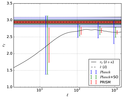
We now assess whether the $\ell$-dependence of the lensing ratio will be measurable using the future experiments discussed here. We find that this dependence will be detectable at the level of 1.4$\sigma$ for $Planck$, 2.2$\sigma$ for $Planck$+SO and 5.1$\sigma$ for PRISM by considering unbinned multipoles. We also visualize the importance of the multipole dependence in Fig. 7, where we display for the Euclid-r1 configuration the errors on $r_{\ell}$ for $Planck$, $Planck$+SO and PRISM, by taking as an example 4 broad bins - see caption for more details. Both the calculation with unbinned multipoles and Fig. 7 show how the multipole dependence induced by lensing magnification could be detected with future experiments.

Figure 8: Contribution of each $\ell$ to the signal-to-noise of $r_{\ell}$ (left panel) and cumulative signal-to-noise as a function of $\ell_{\rm max}$ (center panel) and $\ell_{\rm min}$ (right panel). The solid lines represent the case including only the density term ($\delta$) and the dashed lines correspond to the calculation including also the lensing magnification term ($\delta+\kappa$).

We calculate and show in Fig. 8 the SNR of the lensing ratio for the Euclid-r1 configuration as a function of $\ell_{\rm max}$ and $\ell_{\rm min}$, as well as the individual contribution of each multipole to the total amount. We find that the majority of the information of this estimator is around $\ell\sim 100$. We also find that including corrections from general relativity increases the SNR around $\lesssim 10\%$.

In Tab. 1 we list the SNR of the lensing ratio measurement for the CMB experiments considered as a function of the lens redshift $z_{\rm lens}$ of each bin. We find that the post-$Planck$ CMB lensing will reduce significantly the error on this measurement, reaching up to $\sim 1\%$ with PRISM. We also note the synergies between the Euclid-like survey and the CMB space missions due to the overlapping sky fraction, as an example PICO will be able to measure the lensing ratio with better accuracy than S4 despite having a larger CMB lensing noise. The impact of the lensing correction is stronger at higher $z_{\rm lens}$, allowing to increase the SNR up to a factor $\sim$ 2-3 for the last redshift bin. We have also checked that complementing the ground-based SO and S4 experiments with $Planck$ at $\ell<30$ does not have a significant impact on the SNR.

$z_{\rm lens}$	$Planck$		LiteBIRD		SO		S4		PICO		PRISM
	$\delta$	$\delta$+$\kappa$	$\delta$	$\delta$+$\kappa$	$\delta$	$\delta$+$\kappa$	$\delta$	$\delta$+$\kappa$	$\delta$	$\delta$+$\kappa$	$\delta$	$\delta$+$\kappa$
0.95	18	20	23	25	31	34	55	61	60	67	72	81
1.05	18	20	23	25	30	34	51	59	55	64	64	77
1.15	17	19	22	25	28	33	46	56	50	62	56	72
1.25	16	19	20	25	26	33	40	53	43	58	48	67
1.35	15	19	19	24	23	32	35	50	37	55	40	61
1.45	14	19	17	24	21	30	29	46	30	50	32	54
1.55	12	18	15	23	18	28	23	42	24	45	25	48
1.65	11	17	12	22	15	27	18	37	19	40	19	42
1.75	9	16	10	20	12	25	13	32	14	35	14	36

Table 1: SNR of the lensing ratio for the CMB experiments considered as a function of the foreground redshift $z_{\rm lens}$ for the 9 bins of the Euclid-like spectroscopic survey. We list the SNR calculated using the density term only ($\delta$) and considering also the contribution from lensing magnification ($\delta$+$\kappa$).

VI Cosmological parameter constraints

We investigate here by a Fisher matrix approach whether the measurement of the lensing ratio can help to constrain cosmological parameters in extended models when it is added to the CMB information.

The Fisher matrix formalism astro-ph/9603021 assumes the likelihood $\cal{L}$ to be a multivariate Gaussian and the minimum errors on the cosmological parameters can be estimated from the diagonal of the inverse Fisher matrix ($\sigma_{i}\geq\sqrt{({\cal F}^{-1})_{ii}}$). We define the Fisher matrix of the lensing ratio $r_{\ell}$ as

$${\cal F}_{\alpha\beta}^{r_{\ell}}\equiv\left\langle\frac{\partial^{2}{\cal L}}{\partial\theta_{\alpha}\partial\theta_{\beta}}\right\rangle=\sum_{\ell}\frac{\partial r_{\ell}}{\partial\theta_{\alpha}}\frac{1}{\sigma_{\ell}^{2}(r_{\ell})}\frac{\partial r_{\ell}}{\partial\theta_{\beta}}\,,$$ (47)

where $\theta_{\alpha}$, $\theta_{\beta}$ are the cosmological parameters. The lensing ratio Fisher matrix is added as uncorrelated to the CMB Fisher matrix Jungman:1995bz ; Eisenstein:1998hr , which is given by

$${\cal F}_{\alpha\beta}^{\rm CMB}=\sum_{\ell}\frac{2\ell+1}{2}f_{\rm sky}^{\rm CMB}{\rm Tr}\left[\frac{\partial{\cal C}}{\partial\theta_{\alpha}}{\cal C}^{-1}\frac{\partial{\cal C}}{\partial\theta_{\beta}}{\cal C}^{-1}\right]\,,$$ (48)

where $\cal{C}$ is the 3x3 covariance matrix of the CMB data including temperature ($TT$), polarization ($EE$), lensing ($\phi\phi$) and their cross-correlations.

For the cosmological model, we extend the baseline $\Lambda$CDM+$\sum m_{\nu}$ cosmology to a 9 parameter model where we allow also to vary the dark energy equation of state and the curvature density ($w_{0}$CDM+$\sum m_{\nu}$+$\Omega_{k}$), since we have shown in Section IV that the lensing ratio is sensitive to the variation of these parameters. We adopt as fiducial values $w_{0}$ = -1 and $\Omega_{k}$ = 0.

Figure 9: Marginalized 68% and 95% 2D confidence regions for a $w_{0}$CDM+$\sum m_{\nu}$+$\Omega_{k}$ model obtained by the Fisher matrix of a $Planck$-like experiment including temperature, polarization and lensing (green contours), and adding the Fisher matrix of the lensing ratio obtained using as lens population the first bin of the Euclid-r1 configuration at 0.9 $<z_{\rm lens}<$ 1.0 (blue contours) and the SPHEREx-r1 at 0.2 $<z_{\rm lens}<$ 0.3 (red contours). We do not show the other 5 cosmological parameters since they are not sensitive to the addition of lensing ratio to the CMB information.

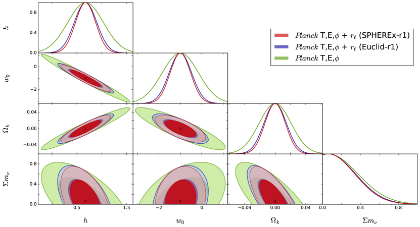
We show in Fig. 9 the 68% and 95% marginalized confidence regions for $h$, $w_{0}$, $\Omega_{k}$ and $\sum m_{\nu}$ obtained for a $Planck$-like CMB experiment following the Fisher matrix described in Eq. (48) and the sum of both $r_{\ell}$ and CMB Fisher matrices. We calculate the $r_{\ell}$ Fisher matrix for the Euclid-r1 and SPHEREx-r1 configurations described in Section III. The improvement found by adding the lensing ratio to the CMB information is about $\lesssim 40\%$ for $h$, $w_{0}$ and $\Omega_{k}$, while the neutrino mass is only marginally improved. For the spatial curvature we get a combined uncertainty of $\sigma(\Omega_{k})\sim 0.015$, comparable to the $Planck$ 2018 1807.06209 error for a simpler $\Lambda$CDM+$\Omega_{k}$ model using CMB temperature and polarization. The constraints from the combination with the lensing ratio obtained with SPHEREx as foreground population are slightly better with respect to the Euclid-like spectroscopic lens.

Figure 10: As for Fig. 9 but using $Planck$+SO as CMB experiment.

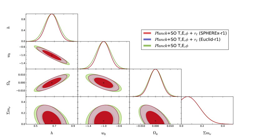
In Fig. 10 we show the same constraints but using $Planck$+SO as CMB experiment. For this case, we find relative improvements around $\sim 15\%$ for $h$ and $w_{0}$ and $\sim$ 10% for $\Omega_{k}$ with respect to the CMB. For the spatial curvature error, we get $\sigma(\Omega_{k})\sim 0.004$ for the combination of SO with Euclid-r1 or SPHEREx-r1.

Figure 11: Predicted bias in the cosmological parameters induced by neglecting the lensing magnification contribution to the galaxy number counts in a combined analysis of the CMB and the lensing ratio, using $Planck$ and the Euclid-r1 configuration. The blue contours represent the marginalized 68% and 95% 2D confidence regions for the $h$-$\Omega_{k}$ and $w_{0}$-$\Omega_{k}$ planes obtained considering the lensing contribution ($\delta+\kappa$), while the red contours correspond to the case with the density term only ($\delta$).

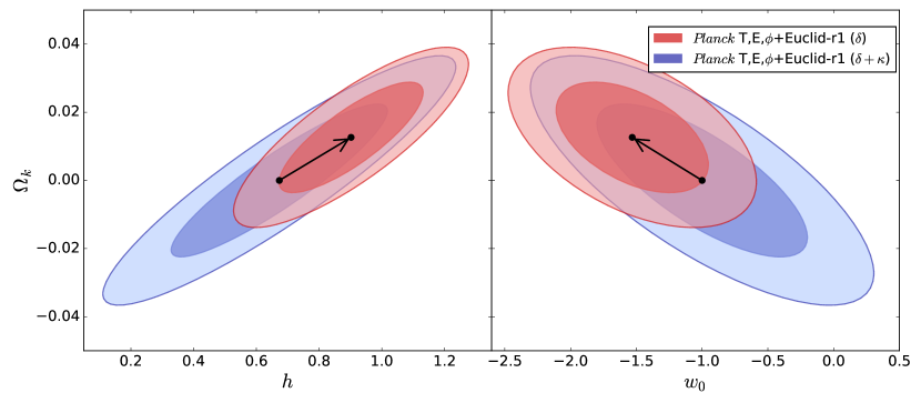
We have shown that the $\hat{r}$ and $\hat{r}_{\ell}$ estimators -which neglect and include the contribution from lensing magnification, respectively- are different in terms of SNR. We now explore whether neglecting the inclusion of the lensing magnification term can induce a bias in the derived cosmological parameters. Following the formalism by Kitching:2008eq , it can be shown the predicted bias in the cosmological parameters due to an uncorrected effect/systematic is expressed as

$$b_{\theta_{\alpha}}=(\widetilde{\cal F}^{-1})_{\alpha\beta}B_{\beta}\,,$$ (49)

where $\widetilde{\cal F}_{\alpha\beta}$ is the Fisher matrix computed by assuming the theoretical signal without the lensing magnification term. The vector $B_{\beta}$ is given by

$$B_{\beta}=\sum_{\ell}\frac{1}{\sigma_{\ell}^{2}(\widetilde{r}_{\ell})}(\widetilde{r}_{\ell}-r_{\ell})\frac{\partial\widetilde{r}_{\ell}}{\partial\theta_{\beta}}\,,$$ (50)

where $\widetilde{r_{\ell}}$ and $r_{\ell}$ are the lensing ratios obtained without and with the lensing magnification contribution, respectively.

By our working assumptions, we compute the bias in the cosmological parameters for the combined constraints from $Planck$ and the lensing ratio using the Euclid-r1 configuration as an example. We represent the result in Fig. 11, where we show the marginalized 68% and 95% 2D confidence regions for the $h$-$\Omega_{k}$ and $w_{0}$-$\Omega_{k}$ planes obtained considering and neglecting the lensing term, and we have shifted the uncorrected contours by the amount given by Eq. (49). We get for the bias on the parameters $b_{h}=0.23$, $b_{w_{0}}=-0.53$ and $b_{\Omega_{k}}=0.013$, which taking into account the uncertainties from both approaches corresponds to a shift of $0.85\sigma$ for $h$, $0.8\sigma$ for $w_{0}$ and $0.7\sigma$ for $\Omega_{k}$. Whereas the forecast uncertainties by lensing ratio alone improve by adding lensing magnification, consistently with the improvement in the SNR shown in Tab. 1, it is clear from Fig. 11 that the forecast uncertainties in $h$-$\Omega_{k}$ and $w_{0}$-$\Omega_{k}$ in combination with the CMB degrade when taking into account lensing magnification. We interpret this effect as a consequence of introducing an improved lensing ratio which goes beyond its only dependence on distances and on background cosmology and therefore worsten the uncertainties on parameters as $h$-$w_{0}$-$\Omega_{k}$. Therefore, the neglection of lensing magnification term could overestimate the constraints achievable with lensing ratios using lenses at the typical redshift of a Euclid-like spectroscopic survey, in which this contribution is important, and would lead to a potential bias in the cosmological parameters.

Figure 12: Marginalized 68% and 95% 2D confidence regions for a $w_{0}$CDM+$\sum m_{\nu}$+$\Omega_{k}$ model forecast by the combination of a $Planck$-like experiment with the Euclid-r1 lensing ratio configuration (grey contours) and the Euclid-$\sum r_{i}$ tomographic analysis (green contours), and by the combination of $Planck$+SO with the Euclid-r1 configuration (blue contours) and the Euclid-$\sum r_{i}$ tomographic analysis (red contours).

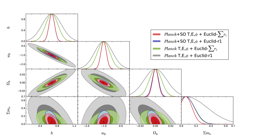
We now explore the possibility of improving the cosmological parameter constraints by combining the 9 possible lensing ratio configurations for Euclid ranging from $z_{\rm lens}=0.9$ to $z_{\rm lens}=1.8$ in a joint tomographic measurement, which hereafter we call Euclid-$\sum r_{i}$. We introduce the covariance of $N$ ratios to take into account that in this combination there is redshift overlap between the different backgrounds and between some backgrounds and foregrounds. We then rewrite Eq. (47) as

$${\cal F}_{\alpha\beta}^{r_{\ell}}=\sum_{\ell}\sum_{i,j}^{N}\frac{\partial r_{\ell}^{i}}{\partial\theta_{\alpha}}[{\rm Cov}(\hat{r}_{\ell})]^{-1}_{ij}\frac{\partial r_{\ell}^{j}}{\partial\theta_{\beta}}\,,$$ (51)

where the $i,j$ indices run over the ratios and the elements of the covariance matrix Cov$(\hat{r}_{\ell})_{ij}$ are given by

$${\rm Cov}(\hat{r}_{\ell})_{ij}=\frac{1}{(2\ell+1)}\frac{1}{C_{\ell}^{\kappa_{\rm gal}^{i}G^{i}}C_{\ell}^{\kappa_{\rm gal}^{j}G^{j}}}\\ \times\bigg{[}\frac{1}{f_{\rm sky}^{\kappa_{\rm CMB}G}}\Big{(}\bar{C}_{\ell}^{\kappa_{\rm CMB}\kappa_{\rm CMB}}\bar{C}_{\ell}^{G^{i}G^{j}}+C_{\ell}^{\kappa_{\rm CMB}G^{i}}C_{\ell}^{\kappa_{\rm CMB}G^{j}}\Big{)}\\ +\frac{r_{\ell,0}^{i}r_{\ell,0}^{j}}{f_{\rm sky}^{\kappa_{\rm gal}G}}\Big{(}\bar{C}_{\ell}^{\kappa_{\rm gal}^{i}\kappa_{\rm gal}^{j}}\bar{C}_{\ell}^{G^{i}G^{j}}+C_{\ell}^{\kappa_{\rm gal}^{i}G^{j}}C_{\ell}^{\kappa_{\rm gal}^{j}G^{i}}\Big{)}\\ -r_{\ell,0}^{i}\frac{f_{\rm sky}^{\kappa_{\rm CMB}\kappa_{\rm gal}G}}{f_{\rm sky}^{\kappa_{\rm CMB}G}f_{\rm sky}^{\kappa_{\rm gal}G}}\Big{(}C_{\ell}^{\kappa_{\rm CMB}\kappa_{\rm gal}^{i}}\bar{C}_{\ell}^{G^{i}G^{j}}+C_{\ell}^{\kappa_{\rm CMB}G^{i}}C_{\ell}^{\kappa_{\rm gal}^{i}G^{j}}\Big{)}\\ -r_{\ell,0}^{j}\frac{f_{\rm sky}^{\kappa_{\rm CMB}\kappa_{\rm gal}G}}{f_{\rm sky}^{\kappa_{\rm CMB}G}f_{\rm sky}^{\kappa_{\rm gal}G}}\Big{(}C_{\ell}^{\kappa_{\rm CMB}\kappa_{\rm gal}^{j}}\bar{C}_{\ell}^{G^{i}G^{j}}\\ +C_{\ell}^{\kappa_{\rm CMB}G^{j}}C_{\ell}^{\kappa_{\rm gal}^{j}G^{i}}\Big{)}\bigg{]}\,.$$ (52)

In Fig. 12 we compare the constraints obtained for $Planck$ and $Planck$+SO in combination with the Euclid-r1 configuration to their combination with the tomographic Euclid-$\sum r_{i}$ measurement. For $Planck$, the constraints on $h$, $w_{0}$ and $\Omega_{k}$ are improved around $\sim 40\%$ from the tomography with respect to the single ratio case, this corresponds to a $\sim 60$-70% improvement with respect to $Planck$ alone. We get a joint uncertainty on the spatial curvature of $\sigma(\Omega_{k})\sim 0.008$. The neutrino mass is the most benefited parameter from the tomography, reaching up to a $\sim 60\%$ improvement with respect to the single bin case. For $Planck$+SO, the CMB has a higher relative weight but still the error on $\Omega_{k}$ is improved around $\sim 10\%$ with tomography, while the neutrino mass error is improved around $\sim$ 30%.

VII Conclusions

We have studied the ratio between the galaxy number counts/CMB lensing and the galaxy number counts/galaxy shear cross-correlations as a cosmographic quantity Das:2008am . We have forecast the scientific capabilities of this estimator using a Euclid-like experiment both for the galaxy background as will be measured from the photometric survey and for the galaxy foreground whose redshift will be determined from its spectroscopic survey, and $Planck$, LiteBIRD, SO, S4, PICO and PRISM for the CMB lensing background. A Euclid-like experiment could deliver tomographic measurements of the lensing ratio on the basis of the amount of lenses obtainable from the spectroscopic survey. We have then increased the lever arm in redshift by complementing the Euclid-like specifications with DESI and SPHEREx as galaxy foreground populations at lower redshift than $z_{\rm lens}=0.9$ We have found that using SPHEREx as lens population and post-$Planck$ space missions as PRISM the lensing ratio will be measurable with a $\sim 0.7\%$ uncertainty.

We have also found a non-trivial angular scale dependence in the lensing ratio when going beyond the cosmographic limit Das:2008am , i.e. when exact expressions are considered and relativistic corrections are taken into account. In particular, we show that the contribution from lensing magnification will be important for future experiments, as shown for other ratio estimators (see e.g. Dizgah:2016bgm ; Ghosh:2018ijm ). Nonetheless, we show that the RSD contribution and the Limber approximation do not induce any significant effect. We have found that this angular scale dependence of the lensing ratio will be especially important at higher redshift of the lenses and can be detectable at a statistical significant level with post-$Planck$ CMB lensing in combination with a Euclid-like experiment. The significance level could be increased in a tomographic analysis combining the lensing ratio measurements form different bins. This multipole dependence calls for the introduction of an ensemble of lensing ratios defined $\ell$ by $\ell$, with their corresponding optimal and minimum variance estimators, which we identify. Using this new formalism, we have calculated the total signal-to-noise of the lensing ratio for a Euclid-like spectroscopic foreground including the contribution from the lensing magnification and compared it to the cosmographic limit approach. We have found an improvement in the signal-to-noise that ranges from $\sim 10\%$ to a factor $\sim$ 2-3, depending on the lens redsfhit. The majority of the information on this estimator is found to be around $\ell\sim 100$.

By using this improved estimator we forecast its capability to constrain a non-flat cosmology with non-zero neutrino mass and a redshift-independent parameter of state for dark energy in combination with future CMB experiments. We find that the inclusion of the lensing ratio can reduce by $\lesssim 40\%$ the uncertainties on $H_{0}$, $w_{0}$ and $\Omega_{k}$ from $Planck$. We also predict a non-negligible bias in the estimation of these cosmological parameters caused by neglecting the lensing magnification term in a combined analysis. We find that a Euclid-like experiment in combination with $Planck$ could provide a constraint on the spatial curvature with an uncertainty of $\sigma(\Omega_{k})\sim 0.015$ for the first bin of the spectroscopic survey centered at $z_{\rm lens}=0.95$. By considering a joint tomographic analysis of 9 lensing ratio measurements for a Euclid-like survey between $z_{\rm lens}=0.9$ and $1.8$, the uncertainty on the spatial curvature can be reduced to $\sigma(\Omega_{k})\sim 0.008$ and we get a $\sim 60$-70% improvement in the errors on $H_{0}$, $w_{0}$, $\Omega_{k}$ and $\sum m_{\nu}$ with respect to $Planck$.