Decoding the radial velocity variations of HD41248 with ESPRESSO

Abstract

Context. Twenty-four years after the discoveries of the first exoplanets, the radial-velocity (RV) method is still one of the most productive techniques to detect and confirm exoplanets. But stellar magnetic activity can induce RV variations large enough to make it difficult to disentangle planet signals from the stellar noise. In this context, HD 41248 is an interesting planet-host candidate, with RV observations plagued by activity-induced signals.

Aims. We report on ESPRESSO observations of HD 41248 and analyse them together with previous observations from HARPS with the goal of evaluating the presence of orbiting planets.

Methods. Using different noise models within a general Bayesian framework designed for planet detection in RV data, we test the significance of the various signals present in the HD 41248 dataset. We use Gaussian processes as well as a first-order moving average component to try to correct for activity-induced signals. At the same time, we analyse photometry from the TESS mission, searching for transits and rotational modulation in the light curve.

Results. The number of significantly detected Keplerian signals depends on the noise model employed, which can range from 0 with the Gaussian process model to 3 with a white noise model. We find that the Gaussian process alone can explain the RV data while allowing for the stellar rotation period and active region evolution timescale to be constrained. The rotation period estimated from the RVs agrees with the value determined from the TESS light curve.

Conclusions. Based on the data that is currently available, we conclude that the RV variations of HD 41248 can be explained by stellar activity (using the Gaussian process model) in line with the evidence from activity indicators and the TESS photometry.

1 Introduction

After a substantial growth in the number of exoplanet discoveries, we are now close to reaching the required precision for the detection of Earth-like planets around stars like the Sun. The radial-velocity (RV) method, in particular, has been instrumental for many planet detections and for measuring precise masses for transiting planets. However, detecting low-mass planets in RV time series is not an easy task due to contaminating signals originating from the stars themselves or instrumental effects (e.g. Fischer et al., 2016).

Stellar activity has long been recognised as an important source of RV variations (e.g. Saar & Donahue, 1997; Santos et al., 2000). The presence of active regions (spots and faculae) on the stellar surface can induce RV signals of several $\operatorname{\,m\!\cdot\!s^{-1}}$, which can sometimes mimic planet signals (e.g. Figueira et al., 2010) or make it difficult to accurately characterise the planets’ orbital parameters and masses. Several activity indicators (obtained from the same spectra where RVs are measured or from auxiliary data) have helped in disentangling planetary and activity signals in some favourable cases (e.g. Queloz et al., 2001; Melo et al., 2007). Another approach is to develop sophisticated statistical models of stellar noise, which can efficiently separate the signals coming from different sources (e.g. Rajpaul et al., 2015).

The metal-poor star HD 41248 represents an interesting case in this respect. Using RV data from HARPS, Jenkins et al. (2013) announced the discovery of two super-Earths orbiting this star. The orbital periods of the proposed planets, around $\sim$18 and $\sim$25 days, would place them close to a 7:5 mean motion resonance, with implications for the formation history of this system. Later, Santos et al. (2014) analysed a much larger data set of HARPS RVs and could not confirm the planetary origin of the signals. The 25-day signal was also present in stellar activity indices, and the 18-day signal could not be recovered with significance in the new data.

A third paper from Jenkins & Tuomi (2014) presents the analysis of the same extended HARPS data set and concludes, as before, that the two signals were induced by orbiting planets. The main differences between these works regard the model used to fit the RV data set: Jenkins & Tuomi (2014) used a moving average term (MA, see Section 4) to account for correlated noise and linear correlations with some activity indicators, while Santos et al. (2014) relied on white-noise models.

More recently, Feng et al. (2017) explored the full set of HARPS data again, concluding that the previously claimed $\sim$25-day signal is probably caused by ‘a combination of planetary perturbation and stellar rotation’ while the $\sim$18-day signal is no longer significant and it is only an alias of a $\sim$13-day signal. This new signal was attributed to a planet candidate with a mass of 7.08 $M_{\oplus}$. Feng et al. (2017) used a method based on periodograms which can take into account MA terms and linear correlations with activity indicators but only sinusoidal planetary signals.

In this work, we present new ESPRESSO observations of HD 41248 and analyse the combined HARPS+ESPRESSO dataset. The paper is organised as follows: Section 2, presents the HARPS and ESPRESSO observations of HD 41248, as well as the data reduction steps performed for each instrument. We also analysed TESS observations from the first ten sectors of the mission. In Section 3, the stellar properties are derived from the observed spectra. Section 4 presents the methods to analyse the RVs, and Section 5 shows the results. We discuss our results and conclude in Sections 6 and 7.

2 Observations

In this section, we describe the observations from HARPS, ESPRESSO, and TESS, as well as the data reduction steps for each instrument.

2.1 HARPS

Between October 2003 and January 2014, HD 41248 was observed a total of 230 times with the HARPS spectrograph at the ESO 3.6 m telescope in La Silla (Mayor et al., 2003). Before March 2013, simultaneous wavelength calibration was achieved using a ThAr lamp, whereas after that date, a Fabry-Perot etalon was used. Within the spectral order of 50 (around 5500 Å), the average signal-to-noise ratio (S/N) of the HARPS spectra is 86, with values ranging from 19 to 142.

The very last HARPS spectrum was taken after a major intervention in the instrument which replaced the circular optical fibres for ones with an octagonal section, providing increased scrambling (Lo Curto et al., 2015). This change introduced an RV offset of several $\operatorname{\,m\!\cdot\!s^{-1}}$. With only one measurement it is very difficult to characterise the offset and, thus, this last point (with BJD$\simeq$2457766) was excluded from the analysis.

Santos et al. (2014) also identified two other HARPS spectra with very low S/N or with an abnormal blue-to-red flux ratio. This can occur on nights when the transmission was affected by bad weather (e.g. due to cirrus). These two spectra (at BJD$\simeq$2455304 and BJD$\simeq$2456409) will also be excluded from the discussion below. Nevertheless, we compared the results of our analysis, including and excluding these two spectra, and found no significant differences.

After these cuts, we have a total of 227 HARPS observations, with a time span of more than 10 years. The RVs were extracted from these spectra with the cross-correlation technique, as implemented by the HARPS pipeline. This method cross-correlates the observed spectrum with a weighted mask (in the case of HD 41248, the mask is optimised for a G2 dwarf), giving rise to the cross-correlation function (CCF). The RV is calculated by fitting a Gaussian function to the CCF. The full width at half maximum (FWHM), depth, and bisector of the CCF were also calculated, as they are often used as stellar activity indicators (e.g. Queloz et al., 2001; Figueira et al., 2013; Lanza et al., 2018).

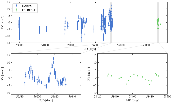
The uncertainties on the RVs include contributions from photon noise, wavelength calibration noise, and the uncertainty in the measurement of the instrumental drift (Bouchy et al., 2001). The full set of HARPS RVs and associated uncertainties are shown in Fig. 1 and listed in Table 5. The average RV error of the 227 observations is 1.41 $\operatorname{\,m\!\cdot\!s^{-1}}$ and the weighted RV standard deviation is 3.54 $\operatorname{\,m\!\cdot\!s^{-1}}$. The ratio between these two values clearly suggests that the RVs contain variations not accounted for by the uncertainties.

2.2 ESPRESSO

The new ESPRESSO spectrograph (Pepe et al., 2014; 2019 in prep.) started operations at the ESO Paranal observatory in September 2018. It is designed and built to reach an unprecedented RV precision of 10 $\operatorname{cm\!\cdot\!s^{-1}}$, with the express goal of detecting low-mass rocky planets within the habitable zones of their host stars. ESPRESSO is a fibre-fed, cross-dispersed, high-resolution échelle spectrograph, combining RV precision and spectroscopic fidelity with the large collecting area of the VLT.

Within the ESO program with ID 0102.C-0757 (PI: J. Faria), we obtained a total of 23 observations of HD 41248 from November 2018 to March 2019. The measurements were taken in ESPRESSO’s high resolution 1UT (HR) mode. With the exception of one observation, which was obtained with UT1, all other spectra were obtained with UT3. We used a Fabry-Perot etalon for simultaneous drift measurement.

Exposure times were set to 15 minutes to average out the p-mode oscillations typical of solar-type stars (e.g. Dumusque et al., 2011; Chaplin et al., 2019). According to the ESPRESSO exposure time calculator (version P102), this would provide a photon noise precision close to 20 $\operatorname{cm\!\cdot\!s^{-1}}$. Around 5500 Å (order 102), the average measured S/N of the ESPRESSO spectra is 165, while the minimum and maximum values are 111 and 201.

As for HARPS, the RVs were extracted from the ESPRESSO spectra with the CCF technique, using the publicly available ESPRESSO pipeline (version 1.2.2, Modigliani et al. 2019). The CCF mask is again optimised for a G2 dwarf, but it is different from that of HARPS as it includes a number of additional lines in the red part of the spectrum, between 6800 Å and 7900 Å, to match ESPRESSO’s larger wavelength coverage.

Line profile indicators were also calculated for each CCF. The average uncertainty on the ESPRESSO RVs is 36.3 $\operatorname{cm\!\cdot\!s^{-1}}$, with an rms of 2.12 $\operatorname{\,m\!\cdot\!s^{-1}}$. We note that the ESPRESSO RV uncertainties only include the photon noise contribution. The RV time series is also shown in Fig. 1 (see Table 5) and compared to the HARPS RVs on the same scale.

Figure 1: Full set of RVs from HARPS (blue) and ESPRESSO (green). Average RV for each data set has been subtracted for visual comparison. The two bottom panels show a zoom on a subset of the HARPS observations (left) and the ESPRESSO observations (right). These two panels are shown on the same scale. We note that all ESPRESSO observations are shown with error bars but in most cases these are smaller than the points.

2.3 TESS

The Transiting Exoplanet Survey Satellite (TESS; Ricker et al. 2015) observes HD 41248 (TIC 350844714, TESS magnitude = 8.187) in sectors one through 13 of its nominal two-year mission. As of June 2018, data from the first ten sectors are available (from 25 July 2018 to 22 April 2019). This leads to a baseline of around 270 days. TESS observations are simultaneous with the ESPRESSO RVs between the end of sector four and middle of sector nine.

We downloaded, combined, and analysed the TESS light curves for the first 10 sectors. An in-depth analysis of the combined light curve is described in Appendix B. In summary, we do not detect credible transit signals. We do find evidence for a stellar rotation period between 24 and 25 days. The data are consistent with a spot lifetime of about 25 days.

3 Stellar characterisation

3.1 Fundamental stellar parameters

HD 41248 (HIP 28460) is a G2V dwarf in the constellation of Pictor, with a visual magnitude of V=8.82. In the Gaia DR2 catalogue (Gaia Collaboration et al., 2016, 2018), its parallax is listed as $18.006\pm 0.028$ mas, leading to a distance of $55.45\pm 0.09$ parsec, as inferred by Bailer-Jones et al. (2018).

Stellar atmospheric parameters were derived using both the HARPS and ESPRESSO spectra. We use the ARES + MOOG method for the spectroscopic analysis (Sousa, 2014). This method is an equivalent width (EW) method, based on the ionisation and excitation balance of Fe I and Fe II lines. The list of iron lines is the same as presented in Sousa et al. (2008). The EWs are automatically measured using ARES (Sousa et al., 2007) and the iron abundances are derived with the MOOG code (Sneden et al., 2012), assuming local thermodynamic equilibrium, and with a grid of Kurucz ATLAS9 models (Kurucz, 1993).

Each HARPS spectrum was shifted by the corresponding RV, after which the flux values in each wavelength bin were added. With the combined spectrum, we derived the following values for the stellar atmospheric parameters: effective temperature T_eff = $5713\pm 63$ K, surface gravity log g = $4.49\pm 0.10$ dex, and metallicity [Fe/H] = $-0.37\pm 0.05$ dex.

The ESPRESSO spectra were combined in a similar way, finally resulting in T_eff = $5724\pm 13$ K, log g = $4.517\pm 0.025$ dex, and [Fe/H] = $-0.348\pm 0.010$ dex. The parameters from HARPS and ESPRESSO agree within the quoted uncertainties. Since ESPRESSO provides higher precision – due to the higher S/N in the combined spectra – we use these values as the final stellar parameters, which are listed in Table 1.

From the stellar atmospheric parameters, we then determined the stellar mass and radius using two methods. First, we used the calibrations from Torres et al. (2010). Uncertainties were derived with a Monte Carlo procedure which resamples the effective temperature, surface gravity, and metallicity using their quoted uncertainties (see Santos et al., 2013). We obtained final values of $0.86\pm 0.06$ $M_{\odot}$ and $0.89\pm 0.04$ $R_{\odot}$, respectively.

As a second method, we derived stellar mass, radius, density, and age with the isochrones package (Morton, 2015) and the Dartmouth stellar isochrones (Dotter et al., 2008). As inputs, we used the apparent magnitudes, the Gaia parallax, and the spectroscopic parameters. This results in an estimated stellar mass of $0.866\pm 0.015$ $M_{\odot}$ and a radius of $0.898\pm 0.005$ $R_{\odot}$, which agree with the values from the calibration but are more precise. For the age, we derive a value of $6.8\pm 0.9$ Gyr (see Table 1).

From a comparison with synthetic spectra, using the code to be described in Costa Silva et al. (in prep.), we also derived the stellar projected rotational velocity, $v\sin i$. The method consists in a $\chi^{2}$ minimisation of the deviations between the synthetic profile (created with MOOG) and the observed spectra, in several wavelength regions where FeI and FeII lines are present. All the stellar parameters are fixed to the values derived previously, except for $v\sin i$, which is set as the only free parameter affecting the synthetic spectra. Our final estimate, using the combined ESPRESSO spectra, is of $2.1\pm 0.8$ $\operatorname{\,km\!\cdot\!s^{-1}}$. Together with the stellar radius, and assuming an inclination of 90^∘, this leads to a rotation period of $22\pm 9$ days.

Table 1: Stellar parameters and elemental abundances for HD 41248.

Parameter	Value	Elem.	Abundance
Spectral type	G2V	C I	$-0.370\pm 0.024$
$V$	8.81	O I	$-0.23\pm 0.07$
$B-V$	0.61	Na I	$-0.311\pm 0.009$
$\pi$ [mas]	$18.006\pm 0.028$	Mg I	$-0.320\pm 0.022$
Distance [pc]	$55.45\pm 0.09$	Al I	$-0.310\pm 0.023$
MV	$5.091\pm 0.011$	Si I	$-0.321\pm 0.031$
L [L⊙]	$0.7871\pm 0.0020$	Ca I	$-0.33\pm 0.06$
$\log{R^{\prime}_{\rm HK}}$	-4.89	Sc II	$-0.32\pm 0.06$
$T_{\rm eff}$ [K]	$5724\pm 13$	Ti I	$-0.305\pm 0.031$
$\log{g}$	$4.517\pm 0.025$	Cr I	$-0.352\pm 0.028$
${\rm[Fe/H]}$	$-0.348\pm 0.010$	Ni I	$-0.391\pm 0.021$
$v\sin i$ [$\operatorname{\,km\!\cdot\!s^{-1}}$]	$2.1\pm 0.8$
Mass $[M_{\odot}]$	$0.866\pm 0.015$
Radius $[R_{\odot}]$	$0.898\pm 0.005$
Density $[\rho_{\odot}]$	$1.197\pm 0.033$
Age [Gyr]	$6.8\pm 0.9$

We also derived abundances of several elements using the same tools (ARES and MOOG) and models (Kurucz ATLAS9) as for the determination of atmospheric parameters. For details on the methods, see Adibekyan et al. (2012), Adibekyan et al. (2015), Delgado Mena et al. (2010), and Bertran de Lis et al. (2015). The derived abundances, measured relative to the Sun, are also listed in Table 1.

3.2 Activity indices

The HARPS and ESPRESSO spectra can be used to calculate several activity indices based on the flux in the cores of the Ca II H and K, H$\alpha$, and Na I D₂ activity-sensitive lines. These indices will be defined here as $\rm I_{\rm Ca\,II}$, $\rm I_{\rm H\alpha}$, and $\rm I_{\rm Na\,I}$, respectively.

We used the open-source package ACTIN (Gomes da Silva et al., 2018) which calculates the activity indices by dividing the flux in the core of activity-sensitive spectral lines by the flux in nearby reference regions. The code can calculate multiple indices with a given number of lines, provided that the line bandpasses fall in the instrument’s wavelength range. The fractions of pixels inside the band-passes are also taken into account (for details, see ACTIN’s documentation).

An index $I$ is calculated using the expression

$$I=\sum_{\ell}\sum_{r}\frac{F_{\ell}}{R_{r}},$$

where $F_{\ell}$ is the flux in the bandpass centred on the line $\ell$, $R_{r}$ is the flux in the bandpass centred at the reference region $r$. The errors of the fluxes are considered as Poisson noise, scaling with $\sqrt{N}$, where $N$ is the photon count in the bandpass. The error of a given index is calculated via error propagation and is given by

$$\sigma_{I}=\frac{\sqrt{\sum_{\ell}\sigma_{F_{\ell}}^{2}+I^{2}\,\sum_{r}\sigma_{R_{r}}^{2}}}{\sum_{r}R_{r}},$$

where $\sigma_{F_{\ell}}$ and $\sigma_{R_{r}}$ are the Poisson (photon) errors of the fluxes $F_{\ell}$ and $R_{r}$, respectively.

In this work we used the same lines and bandpass parameters as in Gomes da Silva et al. (2011), except for $\rm I_{\rm Ca\,II}$ for which we used a triangular bandpass with a FWHM of 1.09 Å  which simulates the calculation of the Mt Wilson $S$-index (Vaughan et al., 1978). Since we are analysing only one individual star and a calibration to transform the Ca II index to the $S$-index scale is still not available for ESPRESSO, we have not computed the photospheric-corrected $R^{\prime}_{\rm HK}$ index (Noyes et al., 1984).

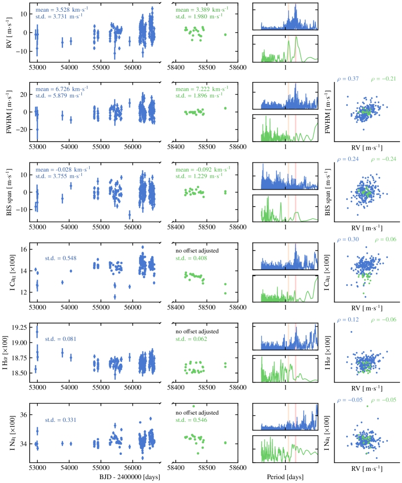
Figure 2 shows the time series of RVs, FWHM, bisector span, $\rm I_{\rm Ca\,II}$, $\rm I_{\rm H\alpha}$, and $\rm I_{\rm Na\,I}$ for ESPRESSO and HARPS. In the case of the RVs, FWHM, and bisector span, an offset between the two instruments was adjusted, since the absolute value of these observables should have an instrumental dependence. The average values of each quantity before adjusting this offset are also shown in the panels and presented in Table 2.

Table 2: Offsets between HARPS and ESPRESSO.

Quantity	HARPS	ESPRESSO	offset
	mean	mean	HARPS - ESPRESSO
	$[\operatorname{\,km\!\cdot\!s^{-1}}]$	$[\operatorname{\,km\!\cdot\!s^{-1}}]$	$[\operatorname{\,m\!\cdot\!s^{-1}}]$
RV	3.52808	3.38867	139.41
FWHM	6.7258	7.22179	-495.99

The Bayesian Generalised Lomb-Scargle (BGLS) periodograms (Mortier et al., 2015) of the different quantities are shown in the middle panels, individually for HARPS and ESPRESSO, and the right panels show the correlation between the RVs and the other variables, with an indication of Pearson’s coefficient of correlation.

Figure 2: Left: Time series of RVs, CCF FWHM, CCF bisector span, $\rm I_{\rm Ca\,II}$, $\rm I_{\rm H\alpha}$, and $\rm I_{\rm Na\,I}$ for HARPS (blue) and ESPRESSO (green). The vertical scales are the same in both broken panels. For the RVs, FWHM, and BIS span an offset between the two instruments was adjusted and subtracted. The average values before this offset are shown in the panels. Middle: Bayesian Lomb-Scargle periodograms of the HARPS and ESPRESSO observations. The red lines indicate the periods of 13.3 and 25.6 days. Right: Correlation of each activity indicator with the RVs, showing Pearson’s correlation coefficient individually for the two instruments.

4 Analysis of the radial velocities

To analyse the two RV data sets, we will consider, in turn, white and correlated noise models. Details on the models and the inference procedure are given below.

4.1 RV model

As a common component of both white and correlated noise models, we assume that the RV variations caused by planets can be modelled as a sum of Keplerian curves. Each Keplerian can be described with five parameters: the semi-amplitude $K$, the orbital period $P$, the eccentricity $e$, the time of periastron $T_{p}$, and the argument of periastron, $\omega$. A model with $N_{p}$ planets corresponds to the sum of the $N_{p}$ individual Keplerian curves.

The RV zero-point corresponds to the radial velocity of the centre of mass of the system, here denoted by $v_{\rm sys}$. Since the RVs come from two instruments, we need to account for an offset, denoted $\delta$ here, between the HARPS and ESPRESSO measurements. In order to model any long-term trends present in the RVs, we also include a linear term (with slope $\beta$ and referenced to $t_{\rm ref}$, the average time of the observations) which is shared between the two instruments.

In summary, for a model with $N_{p}$ planets, the model for the RV of the star at time $t$ is calculated as

$$v(t)=v_{\rm sys} +\delta\,{\rm I}_{\,t\,\in\,\rm ESP}+\beta(t-t_{\rm ref})$$

$$+\sum\limits_{\scriptscriptstyle i=1}^{\scriptscriptstyle N_{p}}K_{i}\left\{\cos\left[\omega_{i}+f_{i}(t)\right]+e_{i}\cos\omega_{i}\right\}$$ (1)

where ${\rm I}_{\,t\,\in\,\rm ESP}$ is an indicator variable equal to 1 if time $t$ belongs to the ESPRESSO data set and 0 otherwise, and $f_{i}(t)$ is the true anomaly for planet $i$, which can be calculated from the other orbital parameters (see e.g. Perryman, 2014).

In addition to the Keplerian signals, the measured RVs can include variations originating from other sources, namely stellar activity or instrumental noise. Here we formulate three different models for these sources of noise by defining the appropriate likelihood function or adding an additional term to Eq. 1.

As a simple white noise model, for a data set $\mathcal{D}$ containing times $t_{k}$, radial velocities $v^{\rm obs}_{k}$, and uncertainties $\sigma_{k}$, we use an independent Gaussian likelihood

$$\mathcal{L}(\theta)=\prod_{k}\frac{1}{\sqrt{2\pi\left(\sigma_{k}^{2}+s^{2}\right)}}\exp\left[-\frac{\left(v^{\rm obs}_{k}-v(t_{k})\right)^{2}}{2\left(\sigma_{k}^{2}+s^{2}\right)}\right],$$ (2)

where $\theta$ is a vector containing all the unknown parameters $\left\{v_{\rm sys},\delta,\beta,P,K,e,\omega,T_{p},s\right\}$. The additional white noise component controlled by the parameter $s$ (often called jitter) can accommodate intrinsic stellar variability or instrumental effects which are not included in the RV uncertainties. In practice, we consider individual jitter parameters for HARPS and for ESPRESSO.

A further generalisation is to allow for off-diagonal terms in the Gaussian likelihood, effectively modelling the RVs with a Gaussian process (GP). The log-likelihood is then given by

$$\ln\mathcal{L}(\theta)=-\frac{1}{2}\mathbf{r}^{T}\,\Sigma^{-1}\,\mathbf{r}-\frac{1}{2}\ln\det\Sigma-\frac{N}{2}\ln 2\pi\text{,}$$ (3)

where $\mathbf{r}$ is the vector of residuals, given by $v^{\rm obs}_{k}-v(t_{k})$, and $\Sigma$ is the covariance matrix. This matrix is obtained by evaluating the covariance function (or kernel) of the GP at the observed times. From the many possible choices for a covariance function, the quasi-periodic kernel is the most widely used in the exoplanet literature (e.g. Haywood et al., 2014; Faria et al., 2016; Cloutier et al., 2017), resulting in a covariance matrix of the form:

$$\Sigma_{ij}=\eta_{1}^{2}\exp\left[-\frac{(t_{i}-t_{j})^{2}}{2\eta_{2}^{2}}-\frac{2\sin^{2}\left(\frac{\pi(t_{i}-t_{j})}{\eta_{3}}\right)}{\eta_{4}^{2}}\right]+\left(\sigma_{i}^{2}+s^{2}\right)\delta_{ij}\>\text{.}$$ (4)

In this GP model, $\eta_{1}$, $\eta_{2}$, $\eta_{3}$, and $\eta_{4}$ are free hyperparameters. They correspond, respectively, to the amplitude, timescale of decay, periodic timescale, and level of high-frequency variability in the GP model (see Rasmussen & Williams, 2006). Both $\eta_{2}$ and $\eta_{3}$ may have physical interpretations as the timescale for evolution of active regions in the stellar surface, and the stellar rotation period. The parameter $\eta_{4}$ controls the scale of variability of the GP within one period $\eta_{3}$, with larger values corresponding to more sinusoidal functions. As before, there is one scalar jitter parameter for each instrument, while the remaining parameters are shared.

A third possibility is to consider a first-order moving average (MA) term in the RV model, as done by Jenkins & Tuomi (2014) for HD 41248 and several other authors (e.g. Tuomi et al., 2014; Díaz et al., 2018; Jenkins et al., 2017; Feng et al., 2016). In the MA model, we consider the following additional term added to the right-hand-side of Eq. (1):

$$v(t_{k})=\ldots+\phi\,\exp\left(\frac{t_{k-1}-t_{k}}{\tau}\right)\,r_{k-1},$$ (5)

where $r_{k-1}$ denotes the residuals after subtracting the model from the $(k-1)$th measurement.

This term can account for correlations between consecutive observations, with exponential smoothing over a timescale of $\tau$ days. The amplitude of the correlations is set by the parameter $\phi$, with values between -1 and 1. Both $\phi$ and $\tau$ are free parameters, shared between HARPS and ESPRESSO.

4.2 Prior distributions

We use informative but broad prior distributions for the model parameters. The orbital periods are assigned a log-uniform (often called Jeffreys) prior between one day and twice the time span of the full data set ($\Delta t\sim 5615$ days). We consider modified log-uniform distributions for both the semi-amplitudes and the jitter parameters $s$, limited above by the variance of the RV observations (${\rm var}\>v^{\rm obs}=13.05\operatorname{\,m\!\cdot\!s^{-1}}$) and with an inflection at 1$\operatorname{\,m\!\cdot\!s^{-1}}$. These modified distributions are defined until the lower limit of $0\operatorname{\,m\!\cdot\!s^{-1}}$, which explicitly allows for the Keplerian and additional white noise terms to cancel.

It is also worth nothing the prior for the orbital eccentricities, which is the Kumaraswamy distribution (Kumaraswamy, 1980), with shape parameters $\alpha=0.867$ and $\beta=3.03$. This distribution closely matches the Beta distribution proposed by Kipping (2013), which is used as an approximation to the frequency distribution of exoplanet eccentricities. The Kumaraswamy distribution has a small computational advantage since its cumulative distribution function can be easily evaluated. Other parameters are assigned uniform priors between sensible limits.

For the GP hyperparameters, we use relatively broad priors: uniform distributions in the logarithm of $\eta_{1}$ and $\eta_{4}$, a log-uniform distribution for $\eta_{2}$ and uniform for $\eta_{3}$ between appropriate limits for a solar-like star (see Table 3). The most restrictive of these priors is the one for $\eta_{3}$, associated with the rotation period of HD 41248, which we define between ten and 40 days. In any case, all evidence gathered so far points to these limits being appropriate. We note that the prior for $\eta_{1}$ can be considered too wide given the observed RV dispersion. However, its functional form assigns low probability to large values of the parameter, and we find that our results do not depend strongly on the prior upper limit. The MA parameters $\phi$ and $\tau$ are also assigned broad but meaningful priors. In particular, we allow for $\tau$ to be as large as 100 days to model activity-related signals.

Table 3: Prior distributions for the parameters in the RV model.

Parameter	Unit	Prior distribution
$N_{p}$		$\mathcal{U}\,(0,4)$
$P$	days	$\mathcal{LU}\,(1,2\Delta t)$
$K$	$\operatorname{\,m\!\cdot\!s^{-1}}$	$\mathcal{MLU}\,(1,{\rm var}\>v^{\rm obs})$
$e$		$\mathcal{K}\,(0.867,3.03)$
$M\left[=\frac{2\pi}{P}(t_{0}-T_{\!p})\right]$		$\mathcal{U}\,(0,2\pi)$
$\omega$		$\mathcal{U}\,(0,2\pi)$
$\ln\eta_{1}$	$\operatorname{\,m\!\cdot\!s^{-1}}$	$\mathcal{U}\,(-5,5)$
$\eta_{2}$	days	$\mathcal{LU}\,(1,100)$
$\eta_{3}$	days	$\mathcal{U}\,(10,40)$
$\ln\eta_{4}$		$\mathcal{U}\,(-1,1)$
$\phi$	$\operatorname{\,m\!\cdot\!s^{-1}}$	$\mathcal{U}\,(-1,1)$
$\tau$	days	$\mathcal{LU}\,(1,100)$
$s$	$\operatorname{\,m\!\cdot\!s^{-1}}$	$\mathcal{MLU}\,\left(1,V\right)$
$v_{\rm sys}$	$\operatorname{\,m\!\cdot\!s^{-1}}$	$\mathcal{U}\,(\min v^{\rm obs},\max v^{\rm obs})$
$\beta$	$\operatorname{\,m\!\cdot\!s^{-1}yr^{\,-1}}$	$\mathcal{U}\,(-\frac{\Delta v^{\rm obs}}{\Delta t},\frac{\Delta v^{\rm obs}}{\Delta t})$
$\delta$	$\operatorname{\,m\!\cdot\!s^{-1}}$	$\mathcal{U}\,(-\Delta v^{\rm obs},\Delta v^{\rm obs})$

4.3 Inference

For the analysis of Section 5.1, we will simply maximise the log-likelihood function instead of sampling from the posterior distribution. This was done by combining several of the optimisation methods implemented in the SciPy package (Jones et al., 2001). The GLS periodograms were calculated using the astropy package (Astropy Collaboration et al., 2018).

To sample from the posterior distribution for the model parameters, we use the diffusive nested sampling (DNS) algorithm proposed by Brewer et al. (2011). In addition to posterior samples, DNS also provides an estimate of the Bayesian evidence, $Z$, the constant which normalises the posterior distribution. The value of $Z$ can be used for model comparison (e.g. Gregory, 2011; Feroz et al., 2011). In our case, we may want to compare models with different numbers of planets. For example, for two models with $N_{p}=0$ and $N_{p}=1$, with equal prior probabilities, the logarithm of the Bayes factor is given by

$$\ln\mathcal{B}_{1,0}=\ln Z_{1}-\ln Z_{0}$$ (6)

where $Z_{0}$ is the evidence of the first model and $Z_{1}$ that of the second. The Bayes factor $\mathcal{B}$ is a continuous measure of evidence for (or against) one model relative to another. It can be interpreted with the scale introduced by Jeffreys (1961) – see also Feroz et al. (2011) and Efron & Gous (2001). In short, we require Bayes factors of at least 150 ($\ln\mathcal{B}\simeq 5$) between consecutive models in order to claim a planet detection (Faria et al., 2016). A more conservative criterion would be to require the Bayes factors to reach 1000 ($\ln\mathcal{B}\simeq 6.9$).

All analyses were carried out with kima, an open-source package aimed at the analysis of RV data sets (Faria et al., 2018). The code can calculate the evidence for a model with a given number of planets or estimate the posterior distribution for $N_{p}$. In both cases, the posteriors for the remaining parameters are also estimated in one single run. This includes the parameters of the GP or the MA components.

5 Results

5.1 Pre-whitening procedure

A common procedure for a first analysis of RV data sets is to fit and subtract models with a successive number of Keplerians, assessing statistical significance with the periodogram false-alarm probability (FAP). Using the combined HARPS + ESPRESSO data set, we first consider a white noise model with $N_{p}=0$ and maximise the log-likelihood, as given by Eq. (2). The optimised model is then subtracted from the RV data, and the GLS periodogram is calculated for the residuals. The FAP 10%, 1%, and 0.1% levels are determined by a bootstrap procedure.

In the periodogram of the residuals, the highest peak is at 25.63 days (with FAP $\ll 0.1\%$), surrounded by a forest of peaks. A second region with periods between 10 and 20 days is dominated by a peak at 13.36 days (FAP $\ll 0.1\%$). Some power is also seen between 8 and 9 days, but these peaks are below the 10% FAP level. We note these periods are close to being harmonics of each other (see, e.g. Boisse et al., 2011).

We then repeat the optimisation of the log-likelihood function with a model having $N_{p}=1$. As initial guesses we use the parameters found for the previous model and extract from the periodogram initial guesses for the Keplerian parameters. The resulting maximum-likelihood values for some of the Keplerian parameters are $P=25.61$ days, $K=3.05\operatorname{\,m\!\cdot\!s^{-1}}$, $e=0.41$. The optimised model is then subtracted from the RV data. The periodogram of the residuals does not show any peaks above 1% FAP, with the highest one being at 21.84 days.

Despite the lack of significant peaks, attempting a fit with $N_{p}=2$ results in a solution with orbital periods at $P_{1}=25.62$ days and $P_{2}=13.35$ days. The semi-amplitudes converge to $K_{1}=2.47\operatorname{\,m\!\cdot\!s^{-1}}$ and $K_{2}=1.56\operatorname{\,m\!\cdot\!s^{-1}}$, with a much lower eccentricity for the first signal ($e_{1}=0.08$) and a significant eccentricity for the second ($e_{2}=0.23$).

5.2 Search for Keplerian signals

We continue the analysis of the RVs with a blind search for Keplerian signals on the combined data set using the white noise model. First, we run models with the number of planets $N_{p}$ fixed to 0, 1, 2, 3, and 4, successively. The priors for all parameters are the same in all runs, as listed in Table 3. The estimated evidences for each value of $N_{p}$ are shown in Table 4, together with the Bayes factors between models with consecutive values of $N_{p}$.

Table 4: Logarithm of the evidence and Bayes factors between white noise models for successive values of $N_{p}$.

$N_{p}$	$\ln Z$	$\ln\mathcal{B}_{i+1,i}$
0	$-680.63$
		$44.0$
1	$-636.63$
		$6.44$
2	$-630.18$
		$5.1$
3	$-625.09$
		$2.28$
4	$-622.81$

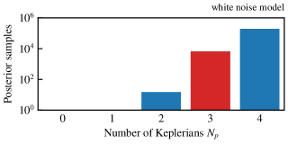
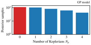
The highest evidence value corresponds to the $N_{p}=4$ model, but the Bayes factors between consecutive models are larger than the detection threshold only up to $N_{p}=3$ ($B_{3,2}$). Therefore, this analysis leads to the significant detection of three signals.

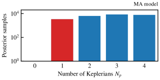
We repeat a similar analysis but with $N_{p}$ free within the uniform prior given in Table 3. Its posterior distribution is shown in the top panel of Fig. 3 and leads to the same conclusion: the significant detection of three Keplerian signals. The final evidence for this model is estimated as $\ln Z=-622.35$.

Figure 3: Posterior distributions for $N_{p}$ from the white noise model (top), the GP model (middle), and the MA model (bottom). The distributions are shown as the number of posterior samples for each value of $N_{p}$ (in logarithmic scale). The red bar highlights the largest value of $N_{p}$ for which the $\mathcal{B}_{i+1,\,i}>150$, corresponding to a significant detection.

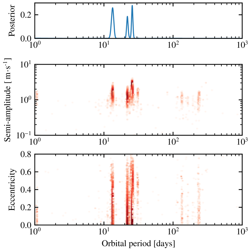
For simplicity, we will now consider only the results from the model with $N_{p}$ fixed to 3. The posterior distributions for the orbital periods, semi-amplitudes and eccentricities are shown in Fig. 4. The three highest peaks in the posterior have periods close to 13.3, 21.8 and 25.6 days and amplitudes around 1.5, 1.2, and 2.7 $\operatorname{\,m\!\cdot\!s^{-1}}$, respectively.

Figure 4: Posterior distributions for the semi-amplitudes, eccentricities and orbital periods within the $N_{p}=3$ model with white noise.

Based on the maximum likelihood solution with $N_{p}=3$, the phase folded Keplerian curves are shown in Fig. 5, together with the residuals for the full data set. The rms of the residuals is of 1.58 $\operatorname{\,m\!\cdot\!s^{-1}}$, which can be compared to the average RV uncertainty of 1.31 $\operatorname{\,m\!\cdot\!s^{-1}}$. Individually for the two instruments, the HARPS residuals show an rms of 2.17 $\operatorname{\,m\!\cdot\!s^{-1}}$ and the ESPRESSO residuals of 0.9 $\operatorname{\,m\!\cdot\!s^{-1}}$. These values are in agreement with the posterior estimated for the jitter parameters: $2.01^{+0.16}_{-0.15}$$\operatorname{\,m\!\cdot\!s^{-1}}$ and $0.86^{+0.23}_{-0.18}$ $\operatorname{\,m\!\cdot\!s^{-1}}$, for HARPS and ESPRESSO respectively.

Figure 5: Phase plots and residuals for the maximum likelihood solution with $N_{p}=3$ and a white noise model. The top panels show the RVs folded at each of the three orbital periods, after removing the contribution from the other two Keplerians. The bottom panel shows the residuals after subtracting the combined signal of the three Keplerians, with an inset showing the ESPRESSO residuals. Data from HARPS and ESPRESSO are colour coded as in Fig. 1, but in the top panels the ESPRESSO points are highlighted. The residual (weighted) rms for the full data set is also shown.

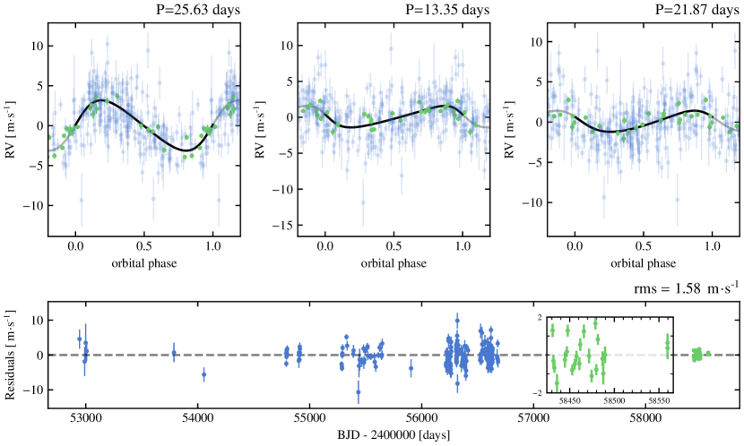
If these three Keplerian signals are caused by planets, their minimum masses can be estimated using this maximum likelihood solution and the value for the stellar mass derived above. This results in 4.5, 12.2, and 5.7 $M_{\oplus}$, for the three periods respectively.

5.3 Including a GP model for stellar activity

We now attempt to model both RV data sets by including quasi-periodic correlated noise. We use the GP model described by Eq. 3 with the kernel from Eq. 4. The number of planets is free and the prior distributions are those of Table 3. After obtaining 100 000 samples from DNS’s target distribution, this corresponds to 34264 posterior samples. The posterior distribution for $N_{p}$ is shown in the middle panel of Fig. 3 and does not result in a significant detection of any Keplerian signals. The final evidence for this model is estimated as $\ln Z=-606.32$.

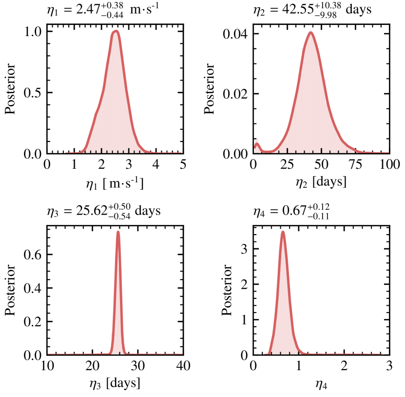
The GP alone is able to reproduce the RV variations of the full data set. The resulting posterior distributions for the hyperparameters of the GP are shown in Fig. 6. For $\eta_{3}$, the posterior is clearly peaked at 25.62 days, which may correspond to the stellar rotation period. The amplitude of the correlations ($\eta_{1}$) is estimated around $2.45\operatorname{\,m\!\cdot\!s^{-1}}$, close to the semi-amplitude of the 25-day Keplerian signal found before. Moreover, $\eta_{2}$ is relatively well constrained around $42.5$ days, which can be physically interpreted as the timescale for active region evolution (e.g. Giles et al., 2017). Finally, the posterior estimate of 0.67 for $\eta_{4}$ means that the RV curve, as modelled by the GP, shows variability on a timescale of about half the stellar rotation period. This can be explained as the active regions on the stellar surface go in and out of view as the star rotates (e.g. López-Morales et al., 2016; Haywood, 2016).

Figure 6: Posterior probability densities for the GP hyperparameters within the model where $N_{p}$ is free. These distributions combine samples from the posterior for all values of $N_{p}$. Each panel also indicates the median and 68% quartiles of the distribution.

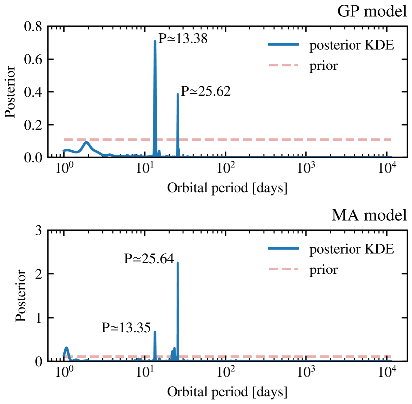
Even if they are not significant enough to provide a detection, the samples with $N_{p}\geq 1$ still have substantial posterior probability within the GP model. The highest peak in the combined posterior for the orbital periods, shown in the top panel of Fig. 7, is around 13.38 days, followed by a peak around 25.62 days. No other period clearly stands out in the posterior distribution. It is important to note that in the samples where $N_{p}\geq 1$, the GP coexists with the Keplerian curves at these two orbital periods. No clear systematic difference is seen in the posteriors for the GP hyperparameters as a function of $N_{p}$, although $\eta_{1}$ decreases slightly with an increasing number of Keplerians.

Figure 7: Posterior for the orbital periods from the GP and MA models. A kernel density estimation (KDE) of the posterior samples is shown together with the probability density function of the prior. We note that the height of the peaks relative to the prior is not a measure of significance.

5.4 Moving average model

In this Section, we consider a second model for correlated noise which uses the MA term from Eq. (5) together with the likelihood from Eq. (2) (and, therefore, no GP). Again, the complete data set is analysed, with $N_{p}$ free within its uniform prior. The MA parameters $\phi$ and $\tau$ are assigned the priors from Table 3 and estimated together with the remaining parameters. These two parameters are the same for HARPS and ESPRESSO.

We obtained 100 000 samples from DNS’s target distribution, resulting in 25689 posterior samples. The final posterior distribution for $N_{p}$ is shown in the bottom panel of Fig. 3, providing evidence for the detection of only one Keplerian signal, according to our detection criterion. Figure 7 (bottom panel) shows the posterior for the orbital periods within the MA model, where the highest peak is again close to 25.6 days, followed by a less significant peak at 13.3 days.

Choosing all samples having $N_{p}=1$ provides the following posterior estimates: orbital period $P=$ $25.61^{+0.01}_{-0.01}$ days, semi-amplitude $K=$ $2.86^{+0.22}_{-0.27}$ $\operatorname{\,m\!\cdot\!s^{-1}}$, and eccentricity $e=$ $0.35^{+0.07}_{-0.09}$. The two MA parameters $\tau$ and $\phi$ do not necessarily have physical interpretations. From the full posterior distribution, $\phi$ is relatively well constrained as $0.27^{+0.17}_{-0.28}$ $\operatorname{\,m\!\cdot\!s^{-1}}$, but $\tau$ is mostly unconstrained within the prior.

6 Discussion

In this Section, we discuss the main implications of our results and attempt to provide a unified explanation for the observed RV variations.

6.1 Clues from the data

Figure 8: Discrete auto-correlation and cross-correlation functions (top and bottom panels, respectively) of the RVs and the FWHM of the CCF for the HARPS data set.

Going back to the beginning, the bottom panels of Fig. 1 show parts of the HARPS and ESPRESSO data sets on a common scale, both in RV and time. The difference in RV precision between the two instruments is clear. What is also evident is that the ESPRESSO RVs show a lower amplitude variation: the HARPS peak-to-peak (PTP) RV variations during this time amount to 19.13 $\operatorname{\,m\!\cdot\!s^{-1}}$, while for ESPRESSO the PTP RV variation is only 7.07 $\operatorname{\,m\!\cdot\!s^{-1}}$. It is unlikely that one single Keplerian signal could cause these variations, even considering instrumental noise.

The BGLS periodograms in Fig. 2 (middle panels) show that both the HARPS and ESPRESSO RVs contain periodicities around 25 and 13 days. We note, however, that the main peak in the periodogram of the ESPRESSO RVs is closer to 28 days, and quite wide. At face value, this could be seen as evidence for one or two planetary companions. However, the HARPS data also show telltale signs of stellar activity: the FWHM of the CCF, the $\rm I_{\rm Ca\,II}$ index, and the $\rm I_{\rm H\alpha}$ index all share the same periodicity close to 25 days.

The ESPRESSO activity indicators do not show the same clear periodicity and also show smaller dispersion, when compared with HARPS. This can be explained if HD 41248 is now at a lower activity level of a long-term magnetic cycle, as suggested by the smaller values and general trend of the $\rm I_{\rm Ca\,II}$ index. If this is the case, and the RV variations are caused by activity, the smaller RV dispersion that we observe with ESPRESSO is expected (see, e.g. Díaz et al., 2016). Part of the additional dispersion on some of the HARPS indicators (e.g. FWHM and BIS) could also be due to photon noise. However, the ratio (HARPS over ESPRESSO) between the standard deviations of the indicators ($\sim$ 3) is higher than the ratio of average S/N in the spectra ($\sim$ 2). Also, the FWHM of the HARPS CCF clearly shows activity-related variations during part of the observations (see Santos et al. 2014). We then attribute the observed smaller dispersion mostly to a quieter stellar activity phase.

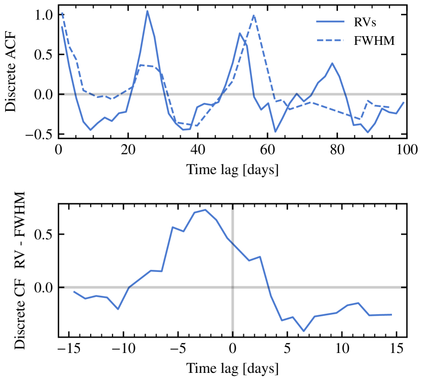
Additionally, the FWHM of the HARPS CCF presents a time lag relative to the RVs, already identified by Santos et al. (2014). We represent this time lag by calculating the discrete auto- and cross-correlation functions between the RVs and the FWHM, using the algorithm from Edelson & Krolik (1988). The results are shown in Fig. 8. The auto-correlation functions show that both RV and FWHM share a similar periodicity around 25 days, as is already evident from the periodograms. The cross-correlation function reveals that the maxima in RV occurs $\sim$3 days before the maxima in FWHM. A very similar behaviour has been recently identified for the Sun (Collier Cameron et al., 2019) and is directly connected to the presence of active regions on the solar surface.

The existence of time lags between the observed RVs and some activity indicators weakens their mutual linear correlations, which explains the small observed values of the correlation coefficients (see Fig. 2, right panels). It may also explain why the model employed by Jenkins & Tuomi (2014) and Feng et al. (2017), which includes these linear correlations, may not be effective at correcting for activity-induced RV signals.

6.2 Results from different noise models

We have analysed the joint RV data set from HARPS and ESPRESSO considering three noise models of different complexity and, for each of them, we estimated how many Keplerian signals are significantly detected in the RV data. The outcome differs from one model to the other: the white noise model, GP model, and MA model lead to the detection of 3, 0, and 1 Keplerian signals, respectively (see Fig. 3). Given these results, we must now compare the models so that we can assess which one (if any) provides a better description of the available data.

Figure 9: Posterior distributions for the additional white noise parameters from the white noise model (top), the GP model (middle), and the MA model (bottom). The distributions for HARPS and ESPRESSO are shown in the same colours as in Fig. 1. Dashed vertical lines correspond to the mean RV uncertainty for each instrument.

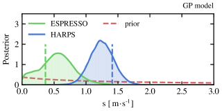
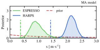
From a purely statistical point of view, the evidence for the GP model ($\ln Z=-606.32$) is significantly higher than for both the white noise ($\ln Z=-622.35$) or the MA ($\ln Z=-623.33$) models. Even though the three models have a different number of free parameters and, thus, different parameter spaces, the value of the evidence can be trusted to provide the most meaningful comparison given the observed data and our priors.

Moreover, the parameters in the GP model can be readily interpreted in physical terms. Our results for all four GP hyperparameters (see Fig. 6) agree with the physical interpretation of a rotating star ($P_{\rm rot}=25.62$ days) with active regions going in and out of view ($\eta_{4}=0.68$) over a lifetime of about two rotation periods ($\sim\!42.55$ days), and an activity-induced RV amplitude that reproduces the observed data. The value for the rotation period matches closely the spectroscopic determination from $v\sin i$ and the estimate from the TESS photometry (see Appendix B). We also note that our estimate for $\eta_{2}$ corresponds to an ‘effective’ lifetime of both spots and faculae. Its relatively large uncertainty may be caused in part by changes in the real lifetime of active regions over the 15 years of observations.

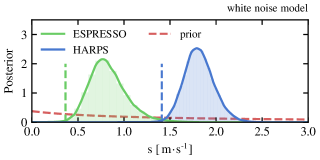
In terms of the RV residuals, our results also point to the GP model being the best description of the data. Figure 9 shows the posterior distributions for the additional white noise parameters for each of the two instruments and each of the three models. These parameters reflect the amount of RV variation observed in the data that is not accommodated by other parts of the models and that must, therefore, be attributed to white, uncorrelated noise. The posteriors are only compatible with the average RV uncertainties (shown as dashed lines in Fig. 9) in the case of the GP model. The results for the additional white noise of ESPRESSO are consistent with the fact that the uncertainties only contain the photon noise contribution and are thus slightly underestimated (by about 18 $\operatorname{cm\!\cdot\!s^{-1}}$, on average).

Regarding the white noise and MA models, we argue that the activity-induced RV signal present in the data is not well modelled with these two noise models. The white noise model can only separate RV variations into Keplerian or white noise components, which leads to a large number of detected signals as well as a high residual rms (see Fig. 5). The moving average term included in the MA model does not seem to be able to account for RV variations over the timescales related to stellar activity, and can only explain a very small part of the observed RV variations. For these reasons, we consider that the results regarding the number and the parameters of the Keplerian signals from these two models are not reliable.

6.3 Detectability limits

Figure 10: Detectability limits from the analysis with the GP model. Black points show posterior samples with $N_{p}\geq 1$ and the orange curve represents the maximum planet mass from those samples, in 300 bins in log-period. Red points are samples from the prior distribution and the diagonal lines correspond to signals with amplitudes of 5, 3, and 1 $\operatorname{\,m\!\cdot\!s^{-1}}$.

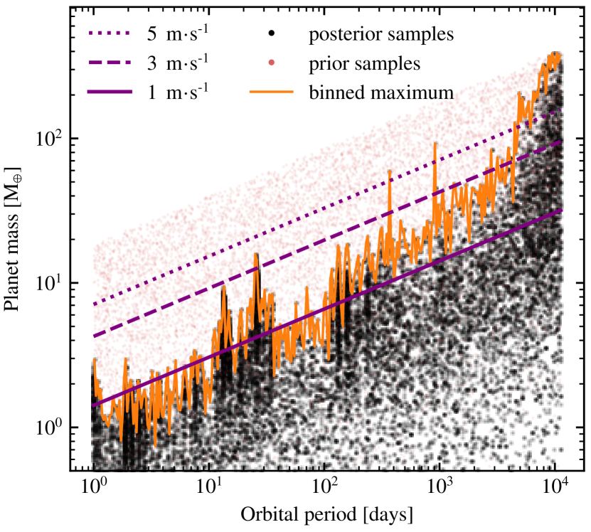
Accepting the GP model as the best explanation for the observed RV variations of HD 41248 leads to the detection of zero planetary companions. However, the currently available data are not sensitive to every possible planet signal. We can use the posterior distributions obtained in our analysis to estimate which planets, in terms of their minimum masses and orbital periods, could still be compatible with the current data and detectable with further future observations.

If we assume that the posterior distribution is sufficiently well explored, the sampler visits the regions of parameter space that contribute substantially to the posterior. Therefore, the resulting samples cover the areas of parameter space which are allowed by the priors and have relatively high likelihood (that is, they are compatible with the data). For samples which have $N_{p}>N_{p}^{\rm detected}$, this means that the sampler visits the highest possible Keplerian amplitudes allowed by the data, as well as amplitudes so low that the data cannot rule them out. The former provide a detectability limit. We note that these limits include the GP stellar activity model.

From all the posterior samples of the GP model, we select those with $N_{p}\geq 1$. With the orbital periods, semi-amplitudes, and eccentricities of these samples (for each of the up to four Keplerians), and the stellar mass given in Table 1, we calculate the minimum mass a planet with those parameters would have. Figure 10 shows all the samples in the planet mass – orbital period space. The maximum mass at each period corresponds to the detectability limit with the current data. Samples from the prior distribution are also shown.

The available data can constrain the posterior at shorter orbital periods but less so for periods longer than the time span of observations (5615 days). The increase in the detectability limits in the region between ten and 40 days is due to the effect of stellar activity, which can conceal more massive planets that would otherwise be detected if stellar activity was not present. The increase in the average level of the detectability limits after orbital periods around 100 days is due to the time span of the ESPRESSO observations (128 days) after which the posterior is constrained mostly by the HARPS data, which have a lower precision.

7 Conclusions

We obtained ESPRESSO observations of HD 41248 with the goal of confirming or disproving the presence of planetary companions around this star. The ESPRESSO RVs show a much improved precision when compared to previous observations from HARPS. Analysis of the full data set with different noise models leads to different conclusions regarding the number of significant Keplerian signals detected in the data.

We conclude that the GP model best explains the observed RV variations because (i) it has a higher evidence when compared to the other models; (ii) it allows for the stellar rotation period and active region evolution timescale to be determined; and (iii) the level of the RV residuals and model jitters agree with the estimated uncertainties for each instrument.

Analysis of the HARPS activity indicators shows clear evidence pointing to the chromospheric origin of the RV variations: some indicators show periodicities in common with the RVs, and the FWHM of the HARPS CCF in particular shows a clear time lag of $\sim\!3$ days relative to the RVs, which is known to be a sign of stellar activity (Collier Cameron et al., 2019). The ESPRESSO activity indicators, on the other hand, show less clear variations and periodicities, which we attribute to a quieter stellar activity phase during the ESPRESSO observations.

Overall, HD 41248 is a telling example of the difficulties introduced by stellar activity when trying to detect planets with RV observations. The presence of several (high amplitude) signals in the RV time series is not up for discussion but their interpretation with relation to orbiting planets is complex. Confirming the presence of a planet is often much harder than simply finding a significant periodic signal. Our conclusion from the currently available data is that they do not provide enough evidence for the detection of a planet and our stellar activity model is both physically interpretable and statistically preferred.

This work presents, for the first time, radial velocities obtained with ESPRESSO. The data clearly show that the instrument is already delivering on the expected RV precision in its first semester of operations. The limited time span of our observations does not allow us to comment on the long-term RV stability but the gain in precision relative to current state-of-the-art spectrographs like HARPS is evident.

In the future, it will be important to develop new activity indicators which can track stellar activity down to this unprecedented $\operatorname{cm\!\cdot\!s^{-1}}$ level (see, e.g. Lanza et al., 2018; Wise et al., 2018). Moreover, extracting RVs using spectral lines less sensitive to activity (e.g. Dumusque, 2018), or joint modelling of the RVs and some activity indicators (Rajpaul et al., 2015; Jones et al., 2017) may also help in disentangling stellar activity from planets.

Appendix A RVs

Table 5 provides the full set of radial velocities and activity indicators from both the HARPS and ESPRESSO observations of HD 41248. The columns are:

1. modified barycentric Julian day (BJD);

2. barycentric RV in $\operatorname{\,km\!\cdot\!s^{-1}}$

3. RV error in $\operatorname{\,km\!\cdot\!s^{-1}}$

4. CCF FWHM in $\operatorname{\,km\!\cdot\!s^{-1}}$

5. CCF bisector span in $\operatorname{\,km\!\cdot\!s^{-1}}$

6. activity index based on the Ca II H & K lines ($\rm I_{\rm Ca\,II}$)

7. activity index based on the H_α line ($\rm I_{\rm H\alpha}$)

8. activity index based on the Na I lines ($\rm I_{\rm Na\,I}$)

9. instrument

Table 5: Radial velocities and activity indicators (full table online-only).

Time	RV	$\sigma_{\mathrm{RV}}$	FWHM	BIS	$\rm I_{\rm Ca\,II}$	$\rm I_{\rm H\alpha}$	$\rm I_{\rm Na\,I}$	instrument
BJD - 2 400 000	[$\operatorname{\,km\!\cdot\!s^{-1}}$]	[$\operatorname{\,km\!\cdot\!s^{-1}}$]	[$\operatorname{\,km\!\cdot\!s^{-1}}$]	[m s-1]	–	–	–
52943.85284	3.52687	0.00275	6.72630	-0.03593	0.14124	0.18564	0.33982	HARPS
52989.71023	3.51946	0.00420	6.72352	-0.02740	0.12679	0.19175	0.34004	HARPS
52998.68982	3.52675	0.00552	6.70572	-0.03353	0.12621	0.18844	0.34867	HARPS
…
58489.58447	3.38982	0.00044	7.21972	-0.09453	0.13210	0.18537	0.34246	ESPRESSO
58559.56959	3.38725	0.00058	7.22624	-0.09247	0.11902	0.18658	0.34051	ESPRESSO
58559.58456	3.38740	0.00049	7.22581	-0.09132	0.12758	0.18602	0.34091	ESPRESSO

Appendix B Analysis of the TESS light curve

The TESS mission is set to observe HD 41248 during the full first year of its nominal two-year mission. Using the Lightkurve package (Lightkurve Collaboration et al. 2018), we downloaded and extracted the Pre-search Data Conditioning (PDCSAP_FLUX) light curves (LC) produced by the Science Processing Operations Center from the Mikulski Archive for Space Telescopes (MAST). As of June 2018, data from the first ten sectors are available, with a baseline of 243 days. The individual LCs were then merged by adjusting the mean of the flux in each sector, and outliers were removed with a 5-sigma-clipping procedure. This results in the merged LC shown in Fig. 11, which also includes an indication of the period where TESS observations are simultaneous with ESPRESSO.

Figure 11: Merged TESS light curve from the first ten sectors. The camera and CCD number with which HD 41248 was observed in each sector is indicated at the top, as well as the period of ESPRESSO observations. The orange points show the binned LC over a 2-hour window.

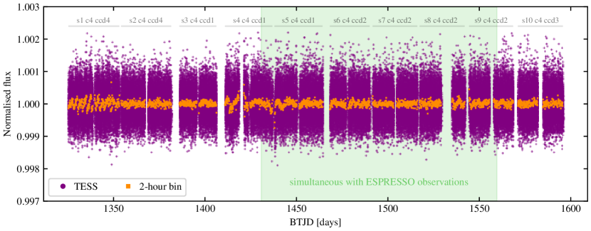
The merged LC shows a weighted rms of 431 ppm. Using the relations between active-region lifetime, spot size, and stellar effective temperature determined by Giles et al. (2017, their Eq. 8). This leads to an estimate of 25.57 days for the decay lifetime of active regions in the stellar surface. This relation was built for star spots, since these have a larger effect in the brightness variations when compared with faculae. In the Sun, faculae tend to live longer than spots (Solanki et al. 2006; Shapiro et al. 2017).

B.1 Transit search

Without performing any additional detrending, we applied the Transit Least Squares (TLS) algorithm (Hippke & Heller 2019) on the merged LC. The TLS algorithm is optimised for detecting shallow transits by using a realistic transit shape with ingress and egress, as well as stellar limb darkening (Mandel & Agol 2002), instead of the box-shaped function used in the more common Box Least Squares (BLS) algorithm (Kovács et al. 2002). The TLS implementation is publicly available, requiring as inputs the stellar limb darkening, mass, and radius. We used the limb darkening estimates available in the TIC catalogue and the mass and radius in Table 1. The output is the so-called signal detection efficiency (SDE) for the trial periods. According to Hippke & Heller (2019), SDE values larger than 7 result in a false-positive rate of 1%.

Figure 12: Left: TLS periodogram for the TESS light curve of HD 41248. Blue line represents the highest peak, at a period of 52.52 days and with an SDE of 10.05. Dashed blue lines show harmonics of this period. Right: Full TESS light curve of HD 41248 with predicted transit curves (black) and in-transit data points (orange) for the highlighted period.

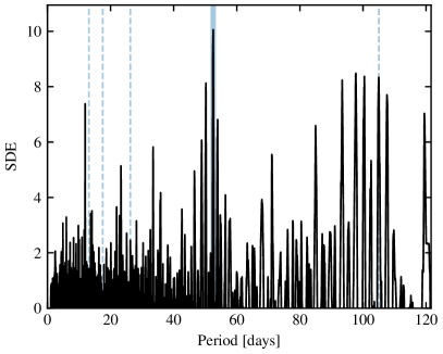
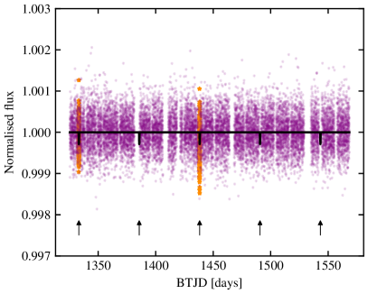
This analysis results in the detection of a significant periodic signal at 52.52 days, with a transit depth of 0.99971 and an SDE of 10.05 (see Fig. 12). However, 3 of the 5 transits are without data because they happen in the beginning or the end of gaps in the LC (mostly between TESS sectors). A visual inspection of the LC together with the predicted transits confirms the occurrence of three transits during gaps (Fig. 12, right panel). One of the predicted transits happens at the start of sector five, where the data show a ramp up lasting about one day. Therefore, although the SDE of this signal should be considered significant, we believe that this is a false positive created by instrumental trends or the detrending procedures applied to the edges of each sector.

We then attempted to detrend the merged LC before repeating a transit search. The detrending aims to filter out as much noise as possible (outliers, stellar variability, residual instrumental signals) while preserving the transit signals. This step is often crucial to enhance the sensitivity of the transit search. For this reason, we tried two slightly different detrending approaches, both following the same scheme: we apply a low pass filter to obtain a smoothed version of the LC. The LC is then divided by the smoothed version and filtered for outliers using a 5-sigma-clipping method. The difference between the two detrending methods is the type of low-pass filter used. First, we used a third order spline filter, with break points every 0.5 days, followed by a 5-sigma-clipping procedure (for details, see Barros et al. 2016). For the second method, we used a Savitzky-Golay filter (as implemented in the lightkurve package) with a window size of 1.4 days and a second order polynomial detrending.

These detrended LCs were then searched for transits with the BLS algorithm. The search was carried out over periods ranging from 0.5 to 97 days (60% of the full duration of the LC). The highest signal in the BLS periodogram, after both detrending methods, is at a period of 28.4 days, but it has a low significance. Visual inspection allows us to discard the possibility of a transit. We conclude that there are no clear signs of transiting planets with periods up to 97 days.

B.2 Rotation period

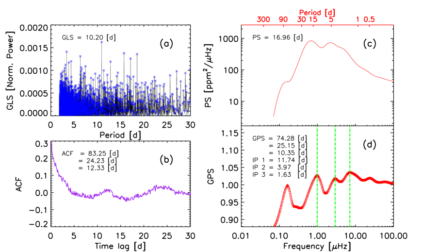
We searched the TESS LC for a periodic signal that can be associated to stellar rotation using four different methods: the GLS periodogram, the autocorrelation function (ACF, e.g. McQuillan et al. 2014), the wavelet power spectra (PS, e.g. Torrence & Compo 1998), and the gradient of the power spectra (GPS, Shapiro et al. 2019; Amazo-Gomez et al., in prep.)

The GPS method in particular attempts to determine the rotation period from the enhanced profile of the high-frequency tail of the power spectrum by identifying the point where the gradient of the power spectrum reaches its maximum value. Such a point corresponds to the inflection point (IP), that is, a point where the concavity of the power spectrum changes sign. Shapiro et al. (2019) show that the period corresponding to the inflection point is connected to the stellar rotation period by a calibration factor equal to $\alpha_{\rm Sun}=0.158$, for Sun-like stars.

The results from the four methods are presented in Fig. 13 and can be summarised as follows: the GLS periodogram suggests a periodic signal of 10.2 days, but with a low relative power; the ACF shows periodic signals at 24.25 days and 12.34 days. The PS, in panel (c), shows two peaks at 16.96 days and 6.15 days. The GPS method shows three enhanced inflection points with enough amplitude to determine three different periodicities. The inflection points at 11.74, 3.97, and 1.63 days correspond to periodic signals at 74.28, 25.15, and 10.35 days after applying the calibration factor $\alpha_{Sun}$.

From the values obtained using the four different methods, we can see that both the GLS and GPS methods detect a periodicity close to 10 days. The strongest signal in the ACF is around 24.25 days, in agreement with the second enhanced signal from GPS, of 25.15 days. The values obtained with the ACF and GPS are close to those obtained from spectroscopy ($v\sin i$) and with the periodicities seen in some activity indicators, suggesting a stellar rotation period for HD 41248 of about 25 days.

Figure 13: Results from the rotation period analysis showing the GLS periodogram (panel a), ACF (panel b), power spectrum (panel c), and GPS (panel d) of the TESS LC. Each panel displays the most prominent periods detected with each method.