lemmatheorem \aliascntresetthelemma \newaliascntcorollarytheorem \aliascntresetthecorollary \newaliascntpropositiontheorem \aliascntresettheproposition
Maximum likelihood estimation of regularisation parameters in high-dimensional inverse problems: an empirical Bayesian approach
Part I: Methodology and Experiments
Abstract
Many imaging problems require solving an inverse problem that is ill-conditioned or ill-posed. Imaging methods typically address this difficulty by regularising the estimation problem to make it well- posed. This often requires setting the value of the so-called regularisation parameters that control the amount of regularisation enforced. These parameters are notoriously difficult to set a priori, and can have a dramatic impact on the recovered estimates. In this work, we propose a general empirical Bayesian method for setting regularisation parameters in imaging problems that are convex w.r.t. the unknown image. Our method calibrates regularisation parameters directly from the observed data by maximum marginal likelihood estimation, and can simultaneously estimate multiple regularisation parameters. Furthermore, the proposed algorithm uses the same basic operators as proximal optimisation algorithms, namely gradient and proximal operators, and it is therefore straightforward to apply to problems that are currently solved by using proximal optimisation techniques. Our methodology is demonstrated with a range of experiments and comparisons with alternative approaches from the literature. The considered experiments include image denoising, non-blind image deconvolution, and hyperspectral unmixing, using synthesis and analysis priors involving the , total-variation, total-variation and , and total-generalised-variation pseudo-norms. A detailed theoretical analysis of the proposed method is presented in the companion paper [27].
1 Introduction
Image estimation problems are ubiquitous in science and industry, and a central topic of research in imaging sciences. Canonical examples include, for instance, image denoising, image deblurring, compressive sensing, super-resolution, image inpainting, source separation, fusion, and phase retrieval [48]. Solving these problems has stimulated significant advances in imaging methods, models, theory, and algorithms [39, 56, 48, 23].
Most image estimation problems are ill-conditioned or ill-posed [39], a difficulty that imaging methods typically address by regularising the estimation problem to make it well posed. This can be achieved in different ways. For example, in the variational framework, regularisation is introduced by using penalty functions that favour solutions with desired structural or regularity properties (e.g., smoothness, piecewise-regularity, sparsity, or constraints), see [23]. In the Bayesian statistical framework, regularisation arises from the use of informative prior distributions that also allow promoting solutions with expected structural or regularity properties [39]. Moreover, regularisation can be explicitly specified, or learnt from data using modern machine learning techniques. We refer the reader to [3] for an excellent introduction to variational, statistical, and machine learning regularisation approaches.
A main difficulty that arises when using any regularisation technique is deciding how much regularisation is appropriate, as different imaging modalities, instrumental setups, scenes, and noise conditions often require using very different amounts of regularisation. The amount of regularisation is usually explicitly controlled by some of the parameters of the model. The difficulty resides in that setting the value of these regularisation parameters a priori is notoriously difficult, particularly in problems that are ill-posed or ill-conditioned where the regularisation has a dramatic impact on the estimated solutions (see [47, 53, 28] and the illustrative example in Figure 1). As a result, there is significant interest in methods for setting regularisation parameters in an automatic, robust, and adaptive way.
Indeed, the developments of methods to automatically set regularisation parameters is a long-standing research topic in imaging sciences. Some methods such as generalised cross-validation [35], the L-curve [44, 37, 16], the discrepancy principle [49, 11] and residual whiteness measures [2, 43] operate by analysing the residual between the observed data and a prediction derived from the observation model. Such methods can perform well in certain imaging problems, but they are mainly limited to cases involving a single scalar regularisation parameter. Alternatively, methods based on Stein’s unbiased risk estimator (SURE) have also received a lot of attention in the late [34, 31, 28]. These methods seek to select the value of the regularisation parameters by minimising SURE-based surrogates of the estimation mean squared error [31, 57, 34]. SURE methods can perform remarkably well in mildly ill-posed or ill-conditioned problems, but they generally struggle with problems that are more severely ill-conditioned or ill-posed [45]. Some recent works also consider learning regularisation parameters from a training dataset of clean images [68], or adopting a bilevel optimisation strategy [15, 41].
Lastly, the Bayesian statistical framework provides two main strategies for addressing unknown regularisation parameters: the hierarchical and the empirical [62, 47]. So far, imaging methods have mainly adopted the hierarchical strategy, where the unknown regularisation parameters are incorporated into the model to define an augmented posterior, and subsequently removed from the model by marginalisation or estimated jointly with the unknown image [18, 56, 53]. This is the strategy that is adopted by most Markov chain Monte Carlo and variational Bayesian approaches reported in the literature (see e.g., [54, 8]).
In this work we propose to adopt an empirical Bayesian approach to estimate the regularisation parameters directly from the observed data in a fully automatic and unsupervised way. We focus on imaging problems that are convex w.r.t. the unknown image and that can be efficiently solved by using modern convex optimisation techniques once the regularisation parameters have been set [48, 23]. In a manner akin to [47, 4], we set regularisation parameters directly from the observed data by maximum marginal likelihood estimation. A main novelty of our work is that this maximum marginal likelihood estimation problem is efficiently solved by using a stochastic proximal gradient algorithm that is powered by two proximal Markov chain Monte Carlo samplers, thus intimately combining the strengths of modern optimisation and sampling techniques. In addition to being highly efficient and delivering remarkably accurate solutions, the proposed method can be readily implemented with the same tools that are used to construct optimisation algorithms to estimate the unknown image by maximum-a-posteriori estimation, namely proximal and gradient operators.
The remainder of the paper is organised as follows. Section 2 defines the class of imaging problems we consider and introduces basic necessary concepts of Bayesian inference. In Section 3 we present the proposed empirical Bayesian method to calibrate regularisation parameters, provide detailed implementation guidelines and discuss connections with hierarchical Bayesian approaches. Section 4 first demonstrates the proposed methodology with a variety of non-blind image deblurring and imaging denoising problems involving scalar-valued regularisation parameters, including an experiment where we also estimate the noise variance. This is then followed by two challenging experiments that require setting vector-valued regularisation parameters, namely sparse hyperspectral image unmixing with the SUnSAL model [38], and image denoising using a Total Generalised Variation regulariser [14], where the parameters have strong dependencies making the estimation problem particularly difficult. We report comparisons with several alternative approaches from the literature, including the discrepancy principle [49], the SURE-based SUGAR method [28], and the hierarchical Bayesian method described in [53]. Conclusions and perspectives for future work are finally reported in Section 5. Additional practical guidelines are postponed to the appendix. We refer the reader to the companion paper [27] for a detailed theoretical analysis of our methodology.
2 Problem Statement
Let and let be a convex compact set. We consider the estimation of an unknown image from an observation related to by a statistical model with likelihood function
| (1) |
where is convex and continuously differentiable with -Lipschitz gradient, i.e. for any , where . This class includes important observation models, in particular Gaussian linear models of the form where and is a -dimensional Gaussian random variable with zero mean and covariance matrix with . We adopt a Bayesian approach and seek to use prior knowledge about to regularise the estimation problem and improve results. We consider prior distributions given for any and by
| (2) |
for some convex and Lipschitz continuous vector of statistics and where we recall that the normalising constant of the prior distribution is given by
| (3) |
Note that controls the amount of regularity enforced. The function is allowed to be non-differentiable in order to include popular models such as for some dictionary with and norm , as well as constraints on the solution space such as pixel-positivity.
Although rarely mentioned in the literature, these widely used prior distributions regularise the estimation problem by promoting solutions for which is close to the expected value , which depends on . Formally, by differentiating (3) and using Leibniz integral rule [55] we obtain that for any
| (4) |
Additionally, because the prior distribution is log-concave, using [12, Theorem 1.2] we have that for any
| (5) |
with . This result establishes that the prior distribution strongly promotes solutions for which with high probability when is large.
Once the likelihood and prior and are specified, we use Bayes’ theorem [62] to derive the posterior for any and
| (6) |
This posterior distribution underpins all inferences about the image given the observed data . In particular, imaging methods typically use the maximum-a-posteriori (MAP) estimator, given for any by
| (7) |
This Bayesian estimator has several favourable theoretical and computational properties (see [52] for a recent theoretical analysis of this estimator). From a computation viewpoint, since the posterior is log-concave, the computation of is a convex optimisation problem that can usually be efficiently solved using modern optimisation algorithms, see [23]. Imaging MAP algorithms typically adopt a proximal splitting approach [24] involving the gradient and the proximal operator of , , see [10, Definition 12.23]. This operator is defined for any and by
| (8) |
The smoothness parameter controls the regularity properties of the proximal operator. As mentioned previously, the regularisation parameter controls the balance between observed and prior information and can significantly impact inferences about the unknown image , especially in problems that are ill-posed or ill-conditioned. In Figure 1, we illustrate the dramatic effect that the value of may have on the recovered image for a deconvolution problem with a total-variation prior. As expected, when is too small the estimated image is very noisy due to lack of regularisation, and when is too large the resulting image is over-regularised.

Lastly, we want to point out that this work focuses on the estimation of and hence assumes that is known, which in Gaussian observation models reduces to the knowledge of the noise variance . This is a standard assumption in the literature (see, e.g., [28, 53]) that is sometimes difficult to verify in practice. To mitigate this issue, Section 4.2.2 explains how to incorporate the estimation of into the proposed scheme and illustrates this modification with an image deconvolution experiment in which and are estimated jointly. The theory that we present in our companion paper [27] also assumes that is known. Although a full generalisation is not possible, we believe that our theory can be extended to provide weaker convergence guarantees for some blind and semi-blind problems by using arguments similar to [26]; this is an important perspective for future work.
3 Proposed Empirical Bayes methodology
3.1 Empirical Bayes estimation
Under an empirical Bayesian paradigm, the regularisation parameter is estimated directly from the observed data , for example by maximum marginal likelihood estimation. That is, we compute
| (9) |
where we recall that the marginal likelihood is given for any by
| (10) |
Given , empirical Bayesian approaches base inferences on the pseudo-posterior distribution , [20], given for any by
| (11) |
Observe that this strategy is equivalent to Bayesian model selection on a continuous class of models parametrised by , where produces the model with the best fit-to-data (under some additional assumptions, provides the best approximation of the true distribution of in a Kullback–Leibler divergence sense, see [72, Section 2] and references therein).
Empirical Bayesian approaches were first considered in the statistical methodology community (see e.g. [60, 20]), which stimulated developments in computational statistics [61, 5, 6] to enable empirical Bayesian inference for general statistical models. This was recently followed by important theoretical works on the validity of the empirical approach and connections to the hierarchical Bayesian paradigm (see e.g. [58, 40, 63]). Unfortunately, this powerful inference strategy is difficult to apply in imaging problems [64] because the marginal likelihood is computationally intractable as it involves two intractable -dimensional integrals, namely (3) and (10), thus making the optimisation problem (9) very challenging. The aim of this paper is to enable empirical Bayesian inference in imaging inverse problems, with a focus on automatic selection of regularisation parameters for convex problems that would be typically solved by using proximal optimisation techniques. More precisely, inspired by [5, 6], we propose a stochastic gradient Markov chain Monte Carlo (MCMC) algorithm to efficiently solve (9) for imaging models of the general form (6), where two main novelties are that we use state-of-the-art proximal MCMC methods [30] to construct a stochastic optimisation scheme that scales efficiently to high dimensions, and that we provide easily verifiable theoretical conditions ensuring convergence (the latter are studied in depth in the companion paper [27]).
The maximum likelihood estimation problem (9) raises natural questions about the uniqueness of , and about the log-concavity of the marginal likelihood , which are important for the convergence of iterative algorithms to compute . In particular, could potentially admit more than one maximiser. However, we have not observed this in practice in any imaging problem. Indeed, because in our experiments , we suspect that the marginal likelihood concentrates sharply around a single maximiser , and is strongly log-concave w.r.t. in the neighbourhood of . These favourable properties can be formally derived under simplifying assumptions (e.g. that is fully separable on [69]). Extending conditions for uniqueness of (9) to more general imaging problems is an important perspective for future work.
Lastly, we note that empirical Bayesian methods have found many applications in machine learning, for example in the context of feature selection (see, e.g., [50, 66, 67]). In this field, the challenges related to high-dimensionality have been mainly addressed by using conditional Gaussian models for which the high-dimensional integrals (3) and (10) become tractable, thus enabling the use of specialised strategies to solve the optimisation problem (9).
3.2 Stochastic gradient MCMC algorithm
We now present the proposed empirical Bayesian method to solve the marginal maximum likelihood estimation problem (9) and set regularisation parameters. As mentioned previously, the main difficulty in solving (9) is that the marginal likelihood function is computationally intractable.
Suppose for now that was tractable and that we had access to the gradient mapping . Recalling that is a convex compact set, we could seek to iteratively solve (9) by using the projected gradient algorithm [24] which is given by with and associated with the following recursion for any
| (12) |
where is the projection onto and is a sequence of non-increasing step-sizes. As mentioned previously, because in imaging problems , the marginal likelihood typically exhibits a single maximiser and is strongly log-concave w.r.t. in the neighbourhood of . Therefore, we expect that (12) would quickly converge.
Since is not tractable, we cannot directly use (12) to compute . However, we can replace with a noisy estimate and consider a stochastic variant of the projected gradient algorithm. In particular, under mild regularity assumptions, using Fisher’s identity (see Appendix A) and the fact that for any , and , , we obtain that for any
| (13) |
Hence, we can use Monte Carlo Markov chain methods to approximate for any .
We consider a stochastic approximation proximal gradient algorithm (SAPG), see [33], where the expectation is replaced by a Monte Carlo estimator leading to the following gradient estimate for any
| (14) |
where is a sample of size generated by using a Markov Chain targeting , or a regularised approximation of this density. Therefore, to compute , we can build a new sequence associated with the following recursion for any
| (15) |
starting from some , and where is a sequence of non-decreasing sample sizes.
Under some assumptions on and on the Markov kernels (see Section 3.3), the errors in the gradient estimates asymptotically average out and the algorithm converges to a maximiser of . More precisely, given , a sequence of non-increasing weights , and a sequence generated using (15), an approximate solution of (9) can be obtained by calculating, for example, the weighted average555 Averaging iterates is standard in stochastic approximation algorithms. Most known convergence results concern the almost sure convergence of towards , or alternatively a weaker convergence in expectation (see, e.g., [9, 59, 6]).
| (16) |
which converges asymptotically to a solution of (9) as (see [6] for details).
Applying this strategy to imaging problems is highly non-trivial for two reasons: i) it requires generating very high-dimensional Markov chains in a way that is computationally efficient; ii) the Markov chains must satisfy a number of complex technical conditions to ensure the convergence of the optimisation scheme (these conditions are related to the stochastic properties of the sequence of errors of the gradient estimates computed from the Markov chains; they are discussed in detail in our companion paper [27]).
In this work, we address these two major difficulties by constructing an SAPG scheme with state-of-the-art unadjusted proximal Markov kernels that are highly computationally efficient and that automatically satisfy the required theoretical conditions. More importantly, we show both theoretically and empirically that a single sample () per iteration is enough to guarantee the convergence of the proposed SAPG scheme. This allows delivering accurate estimates of regularisation parameters in a computationally scalable way and with theoretical guarantees.
More precisely, to construct the SAPG optimisation scheme we use the Moreau-Yoshida Unadjusted Langevin Algorithm (MYULA) [30], which is a state-of-the-art proximal Markov kernel specifically designed for high-dimensional distributions with terms that are log-concave but not smooth. Accordingly, to draw samples from the posterior , we define the Markov chain , starting from , given by the recursion
| (17) |
where is defined by (8), is a smoothing parameter, is a discretisation step-size, and is a sequence of i.i.d. -dimensional zero-mean Gaussian random variables with an identity covariance matrix. For any and , we denote by the Markov kernel associated with the recursion (17). We refer the reader to [30] and to our companion paper [27] for more details about this Markov kernel, particularly concerning its relationship to the Langevin diffusion process and to proximal optimisation methodology.
Lastly, observe that in order to use (15) it is necessary to evaluate . For most models of interest, cannot be computed exactly and needs to be approximated. Hence, we propose three different strategies to address this calculation depending on whether is a homogeneous function or not.
3.2.1 Scalar-valued with positively homogeneous regulariser
For scalar-valued , i.e. , (13) is given for any by
| (18) |
Assume that there exists such that is a positively homogeneous function, i.e. for any and , , and recalling that we have for any
| (19) |
and therefore
| (20) |
Hence, (18) becomes for any
| (21) |
which leads to Algorithm 1 below. We want to point out that many commonly used regularisers are positively homogeneous. For example, all norms such as , , total variation (), nuclear or compositions of norms with linear operators (e.g., analysis terms of the form , where with ) are positively homogeneous. Moreover, powers of norms with exponent are positively homogeneous, and all linear combinations of positively homogeneous functions with the same homogeneity constant , are also positively homogeneous.
3.2.2 Separably homogeneous regulariser
For the special case of separably homogeneous regularisers, Algorithm 1 can be adapted for multivariate . This is because in this class of regulariser, each component of affects independent subsets of the components of . More precisely, assume that is separably homogeneous in the following sense: there exist , pairwise disjoint subsets of and such that for any , is -positively homogeneous with and for any , where for any , . In this case we have for any
| (22) | ||||
| (23) |
Therefore, for any and we get that
Using this property we obtain Algorithm 2, where for any and is the projection onto .
For example, many works in the imaging literature adopt a so-called synthesis formulation where represents the unknown image on some orthonormal wavelet basis with levels666In synthesis formulations represents the unknown image on some basis ; the solution in the pixel domain is given by ., and consider level-adapted regularisations of the form
where are the elements of associated with the th level and . Here, is a separably homogeneous functional as it can be expressed as where, for any , is 1-positively homogeneous and . Notice that the domain in which is represented is not relevant here; Algorithm 2 can be directly applied to any model where is homogenous separable via a change of basis because the same expression for holds.
3.2.3 General case: inhomogeneous regulariser
When g is neither homogeneous nor separably homogeneous, we address the evaluation of numerically by stochastic simulation. Using that is conditionally independent of given , and using identity (4), we express as the difference between two expectations, i.e. for any
| (24) |
We then use two families of Markov kernels that target the posterior and the prior , respectively, within the SAPG Algorithm 3 below.
For any and , the Markov kernel is as defined previously in (17), and the additional Markov kernel is associated with the MYULA algorithm targeting , which defines , starting from , given by the recursion
| (25) |
where are the smoothing parameter and step-size parameter, respectively.
3.3 Implementation guidelines
We now discuss suitable ranges and recommended values for the parameters of Algorithm 1, Algorithm 2 and Algorithm 3. Rather than optimal values for specific models, our recommendations seek to provide general rules that are simple and robust. We also discuss some other considerations related to the implementation of the methods. Please see Appendix B for implementation and troubleshooting guidelines.
3.3.1 Setting the algorithm parameters
Selecting
Our theoretical convergence analysis [27] requires setting ; this is related to the numerical stability of the Markov chains and stems from the fact that bounds the Lipschitz constant of . Within this stability range, controls a trade-off between computational efficiency and accuracy, with larger values of leading to higher efficiency but also to a larger asymptotic bias. Given the dimensionality involved, and that in our experiments we did not observe any significant bias issues, we recommend using a large , e.g., .
Selecting
This parameter controls the regularity of the smooth approximation of within MYULA and hence another trade-off between bias and convergence speed [30]. We have empirically observed that in order to prevent a significant bias it is necessary to set . Within this range, we prefer larger values of to improve convergence speed, at the expense of some bias. We recommend using , as setting increases asymptotic bias without improving convergence speed because of the effect of on .
Selecting and
Since does not affect the kernel targeting the prior, the stability range for is . In our experiments we set . We usually set to have the same level of smoothing in both chains, however one can also use if is much slower than (see Section B.3 and Section B.5 for more details).
Selecting
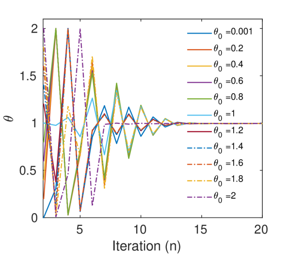
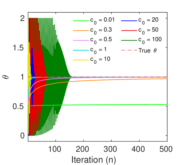
For simplicity and computational efficiency, we recommend using a single () Monte Carlo sample per iteration. A single sample is sufficient to construct a convergent SAPG scheme see our companion paper [27]. We recommend setting with , and use in our experiments, which is a standard choice in the literature [13]. For we recommend, for the case where is scalar, starting with and then adjust if necessary. Although the choice of is asymptotically irrelevant (see Figure 3 (b)), if the initial step-size is too large the iterate will be bouncing on the limits of the interval for a long transient regime, whereas convergence will be slow if is too small. For this reason, we recommend adjusting so that the step-size is of the order of the projection interval . When is not scalar, one can use different scales for each component of . More details are provided in the Section B.4.
Selecting and
While it is possible to construct other estimates, we recommend using the average
| (26) |
with given by
| (27) |
where , . This choice of , defines three distinct phases: i) a burn-in phase where the first iterations of the algorithm are discarded to reduce the non-asymptotic bias (this is particularly important when using a small number of iterations); ii) a uniform averaging phase where the smoothing effect associated with averaging improves convergence speed and reduces estimation variance; iii) a refinement phase where we use decreasing weights to improve the precision of the estimator (see [27] for accuracy guarantees).
We have empirically observed that imaging problems do not usually require highly accurate estimates of . Therefore, in the interest of computational efficiency, in our experiments we omit the third phase and stop when . Moreover, rather than using the theoretical accuracy guarantees of [27] to set , we monitor and stop the algorithms when for a prescribed tolerance (e.g., ).
Selecting
When selecting the projection interval, the lower bound should be as small as necessary but not zero, as this may render the algorithm unstable (the gradient depends on and diverges as ). If possible, use tight bounds to improve convergence speed.
Selecting
The choice of is theoretically asymptotically irrelevant (see, e.g., Figure 3 (a)). However, in some cases a very bad initialisation can prevent the algorithm from converging, e.g., by introducing large numerical errors in the computation of proximal operators. We observed this in the TGV denoising experiment Section 4.4 when using the extreme initialisation (not reported in the paper).
3.3.2 Other implementation considerations
Implementation in logarithmic scale
The proposed algorithms to estimate often exhibit better numerical convergence properties when they are implemented in a logarithmic scale, which is a standard strategy for scale parameters [5]. Accordingly, we introduce the change of variables , obtain an estimate by using one of the proposed algorithms to maximise the marginal likelihood , and then set . This is equivalent to maximising because of the invariance to re-parametrisation property of the maximum likelihood estimator. This change of variables requires a minor modification in the computation of the gradients, which have to be multiplied by to satisfy the chain rule. For example, step 9 in Algorithm 1 becomes , where denotes the range of admissible values of taking the logarithm component-wise. Similarly, step 11 of Algorithm 3 becomes .
Initialisation of the Markov kernels
We strongly recommend warm-starting the Markov chains by running iterations with fixed before starting to update the value of ; an appropriate value for can be easily determined by monitoring the statistic .
Alternative implementations of MYULA
We want to point out that (17) is not the only possible way of implementing MYULA to sample from . If some of the functions are Lipschitz differentiable, it might be convenient to incorporate them through their gradient, and reserve proximal operators for the non-differentiable terms in . Moreover, the above implementation requires computing the proximal operator of the global function . In some cases it might be easier to use the proximal operators of each individual independently (see [30]). Which implementation of MYULA is the most convenient, will mostly depend on the tools available to the practitioner. Many optimisation algorithms for MAP estimation (7) also use the operators and either or [24, 36], making the implementation of our methods straightforward for problems currently solved with such tools. Our theoretical analysis [27] also considers implementations of Algorithm 1, Algorithm 2 with other proximal Markov kernels. Moreover, although for simplicity here we use constant values for , and , the theory presented in [27] allows implementing the algorithms with iteration-dependent values .
Estimation bias
Lastly, as mentioned previously, Algorithm 1, Algorithm 2, and Algorithm 3 can exhibit some asymptotic estimation bias. This error arises from the fact that the MYULA kernels used do not target the posterior or prior distributions exactly but rather an approximation of these distributions [30]. This error is controlled by and , and can be made arbitrarily small at the expense of additional computing time, see [27]. The bias can be completely removed by using iteration-dependent smoothing and step-size parameters and letting them vanish as , but this can dramatically deteriorate the non-asymptotic convergence properties. The bias can also be completely removed by combining MYULA with Metropolis-Hastings (MH) steps, as discussed in detail in [51]. However, it is difficult to calibrate high-dimensional MH steps within a SAPG scheme to achieve the required acceptance rates, as the target densities change at each iteration, so we do not explore this any further. A high-dimensional MH correction can also deteriorate the non-asymptotic convergence properties of the algorithms and significantly increase computing times [30].
3.4 Connections to hierarchical Bayesian approaches
As we mentioned earlier, the Bayesian framework provides two main paradigms to select automatically: the empirical (already discussed in Section 3.1) and the hierarchical, which is currently the predominant Bayesian approach in data science (see [54, 53] for examples in imaging sciences). We now discuss connections between the two paradigms and stress advantages and disadvantages.
In the hierarchical Bayesian paradigm, is modelled as an additional unknown quantity and it is assigned a prior distribution . This leads to an augmented posterior given for any and by
| (28) |
There are two main ways of employing this augmented posterior. The first, and most popular, is to remove from the model by marginalisation, followed by inference on with the marginal posterior given for any by
| (29) |
The marginal posterior is then often used to perform minimum mean squared error (MMSE) estimation by computing
| (30) |
This can be achieved with a standard MCMC algorithm when is tractable, e.g. Gibbs sampling, or with specialised algorithm that allows circumventing the evaluation of at the expense of significant additional computational cost (see [54] for details). For some specific models it is also possible to compute an approximate marginal MMSE solution by using a deterministic variational Bayesian algorithm (e.g., see [7, 46]), but such algorithms have not yet been widely adopted because their implementation and performance remains very problem-specific.
Alternatively, for the class of models considered in Section 3.2.1, one can also efficiently compute the marginal MAP estimator
| (31) |
by using the majorisation-minimisation algorithm proposed in [53]. In some of our experiments we report comparisons with this the hierarchical Bayesian method, as it can be broadly applied to same models as algorithm 1 and algorithm 2.
In order to understand the connection between this hierarchical Bayesian approach and the empirical Bayesian strategy used in this paper it is useful to express as follows
| (32) |
where we observe that is effectively a weighted average of all the posteriors parametrised by , with weights given by the marginal posterior , which represents the uncertainty in given the observed data . If instead of we perform the integration of with respect to the Dirac distribution , we obtain the empirical Bayesian pseudo-posterior considered in this paper.
Note that in imaging problems the marginal posterior will be dominated by the marginal likelihood because of the dimensionality of . Therefore most of the mass of will be close to . As a result, we expect that both the hierarchical and the empirical approaches will deliver broadly similar results. For models that are correctly specified both strategies should perform well, and hierarchical Bayes should moderately outperform empirical Bayes as it is decision-theoretically optimal [62].
However, most imaging models are over-simplistic and hence somewhat misspecified. Our experiments suggest that in this case the empirical Bayesian approach can outperform the hierarchical one. More precisely, we practically observe that the marginal posterior typically has its maximum at a good value for , but struggles to concentrate and spreads its mass across a much wider range of values of . Consequently, fails to sufficiently penalise poor models, which are given too much weight in as a result. In this situation, the pseudo-posterior often delivers better inferences than the marginal posterior . In the context of inverse problems, this phenomenon is particularly clear in problems that are poorly conditioned and where the misspecification of the prior has a stronger effect on the inferences. This behaviour is observed in all the imaging problems reported in Section 4 and is particularly clear in the hyperspectral unmixing problem.
It is also worth mentioning at this point that there is another hierarchical Bayesian approach where and are estimated jointly from , without marginalisation [73, 53]. For example, one can perform joint MAP estimation
| (33) |
This strategy has been studied in detail in [19, 17] in the context of hierarchical Bayesian sparse regularisation models. More precisely, these works cleverly exploit the conditional structure of certain hierarchical Gaussian models with random prior covariance matrices to propose a simple iterative alternating scheme to compute the joint MAP estimator of and the prior covariance. This kind of scheme yields good results for the class of imaging models in those works, both in terms of accuracy and computational complexity. The generalisation of the ideas of [19, 17] to other imaging models, particularly the class of models considered in this paper, is very interesting but highly non-trivial.
4 Numerical experiments
In this section we validate the proposed methodology with a range of imaging inverse problems, which we have selected to illustrate a variety of observation models and regularisation functions. The first experiment, presented in Section 4.1, is carried out using synthetic images for which the exact generative statistical model is known, as this allows assessing the performance of the proposed method in a case where the regularisation parameter has a true value, and where there is no model misspecification. We also use this experiment to explore the robustness of the method towards mild likelihood misspecification (e.g., when there is a mismatch in the statistical properties of the noise).
Following on from this, in Section 4.2 we demonstrate the method by estimating a scalar-valued regularisation parameter in a non-blind image deconvolution model with different kinds of prior distributions, such as total variation and -wavelet priors. This allows comparing our method to some state-of-the-art approaches that are limited to scalar-valued regularisation parameters. We also use one of these experiments to explain how to address problems in which the noise variance is unknown by jointly estimating and the variance of the noise by marginal MLE.
This is then followed by two challenging problems involving multivariate regularisation parameters. In Section 4.3 we apply our method to a sparse hyperspectral unmixing problem combining an and a total variation regularisation, and where we report comparisons with the hierarchical Bayesian approach of [53]. Lastly, in Section 4.4 we apply our method to a total generalised variation denoising model that has two unknown regularisation parameters exhibiting strong dependencies, and which requires using Algorithm 3 with two parallel Markov chains.
In all the experiments we first compute , see (16), and then calculate a MAP estimator using the empirical Bayesian posterior by convex optimisation (solver details are provided in each experiment). All experiments were carried out on an Intel i9-8950HK@2.90GHz workstation running MATLAB R2018a. In all experiments, was estimated on a logarithmic scale by using the change of variables discussed in Section Section 3.3.2, except for the first experiment in Section 4.1 where we used a linear scale.
4.1 Performance on synthetic images - denoising
We first demonstrate the performance of the algorithm on a very simple image denoising problem, where we work with synthetic test images to have access to the true value of the regularisation parameter. We consider a wavelet-based image denoising under a synthesis formulation where we assume that the coefficients of the true image in an orthogonal 4-level Haar basis follow a Laplace distribution. That is the model (6) is given for any by and . In our experiments, has dimension pixels, and we set to generate the synthetic test images. The variance of the added noise is chosen for every case such that the signal-to-noise-ratio () is , , or . In all cases we compute the empirical Bayes estimator by implementing Algorithm 1 with the MYULA kernel (17).
To study the statistical behaviour of the method, we repeat each experiment 500 times by generating 500 random observations , each one coming from a different random ; then, for every observation , we estimate .
(a) =20

(b) =30

(c) =40
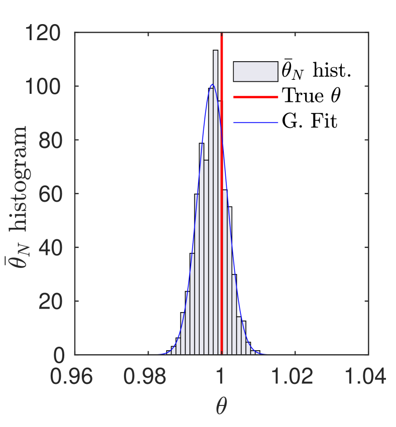
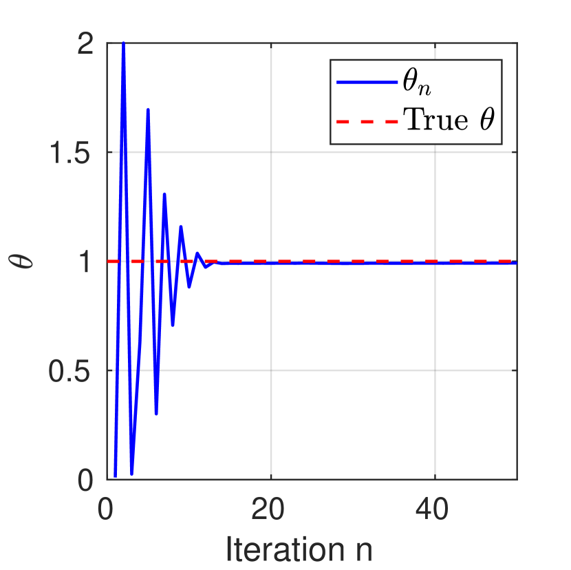
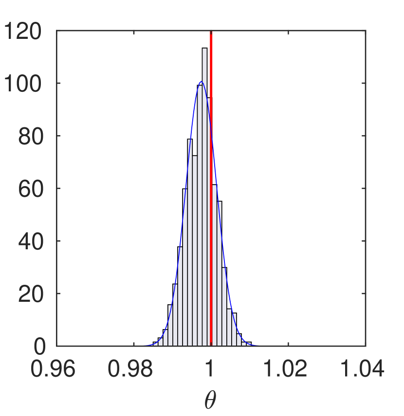
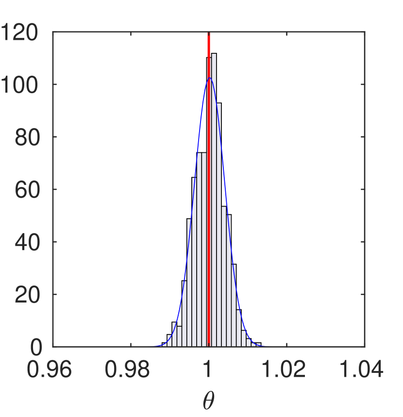
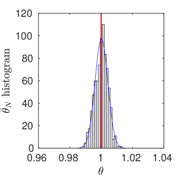
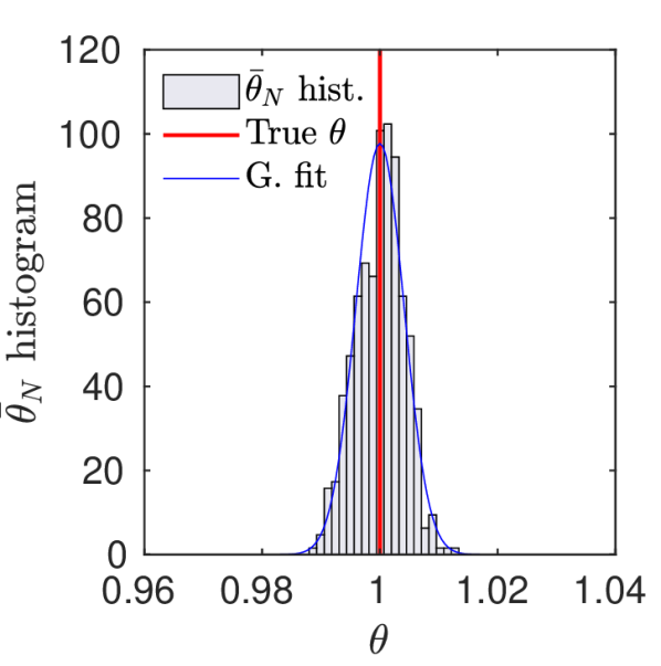
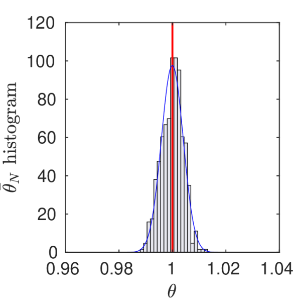
Figure 2 shows the histograms obtained from the 500 estimated values for each experiment (, , and ). For completeness, we also present in Figure 2 one example of a generated sequence of iterates for each experiment. Observe that the estimation error is close to Gaussian and close to the true value of the regularisation parameter, as expected for a maximum likelihood estimator. The algorithm converges in approximately 15 iterations, possibly with some very small bias of the order of .
To illustrate the robustness of the methods w.r.t. the initialisation parameters and , we show in Figure 3 (a) and (b) the evolution of the iterate for different values of and , respectively. Observe that all sequences converge to the same solution, and that with an appropriate choice of the scheme is robust to the choice of . Also observe that a poor choice of can dramatically reduce convergence speed.
(a)
(b)
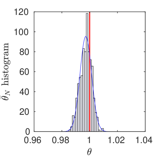
Moreover, to explore the behaviour of the method with other noise distributions, we repeat the previous experiment using Laplace noise instead of Gaussian noise. Since the Laplace distribution involves a non-smooth term, we adopt a proximal MCMC approach and implement the algorithms using the gradient of its -Moreau-Yosida envelope. The results are reported in Figure 4 (a).

=20
(b) Gaussian noise model (a) Laplace noise model

=30
=40
Lastly, to explore the robustness of the method towards mild misspecification of the likelihood, we have also repeated the same experiment with Laplace noise but using an incorrectly specified Gaussian noise model. These results are reported in Figure 4 (b), where we see that the method is robust to mild likelihood misspecification, as the differences between using a correctly specified likelihood or an incorrectly Gaussian likelihood only become noticeable for the lowest SNR of 20 dB.
4.2 Non-blind natural image deconvolution
We now illustrate the proposed methodology with an application to image deblurring using two different kinds of prior distributions: the total variation () prior and a wavelet-based synthesis- prior. For comparison, we also report the results obtained with [28] (only when using a prior), joint MAP estimation [53], discrepancy principle [32, 49], and by using the oracle value that minimises the estimation mean squared error (), i.e.
| (34) |
where is the ground truth. We want to highlight that carrying out such a comparison is not a trivial task because some algorithms are solver-dependent while some others are completely independent of the solver used to compute the MAP estimator. For this reason, the comparison was done with extreme care, and we include a detailed explanation of how we compare the results in Appendix C.
In non-blind image deblurring, the aim is to recover an unknown image from a blurred and noisy observation , where is a blur matrix, and is a Gaussian random variable with zero mean and covariance matrix with . In our experiments, and are of size pixels, is a known circulant uniform blur of size pixels, and is chosen such that the blurred signal-to-noise-ratio () is , , or . We perform all experiments on ten standard test images (barbara, boat, bridge, flintstones, goldhill, lake, lena, man, mandrill and wheel).
For each image, noise level, and selection method, we first obtain an estimate for and then use it to compute the MAP estimator (given by (7)). In the case of the joint MAP method [53], we carry out joint MAP estimation of and . We compute the MAP estimator by using a highly efficient proximal convex optimisation algorithm, SALSA [1], which is an instance of Alternative Direction Method of Multipliers (ADMM). We then assess the resulting performance by computing the between the estimator and the ground truth.
4.2.1 Deconvolution with Total Variation prior
In this experiment we use model (6) where for any we have , , and follow the previously explained procedure. Here is the isotropic total variation pseudo-norm given by where and denote horizontal and vertical first-order local difference operators. To compute we use Algorithm 1. The prior associated with the total variation pseudo-norm is not proper, so the effective dimension is . We evaluated the proximal operator of using the primal-dual algorithm from [22] with 25 iterations.
The algorithm parameters are chosen following the recommendations provided in Section 3.3.1; we consider warm-up iterations and set , , and for any ; we set with and , and . As suggested in Section 3.3.1, we set to have burn-in iterations and compute using (16).
In addition, instead of setting a fixed number of iterations, we stop the algorithm when the relative change is smaller than . It would be possible to use a tolerance of and get a slight improvement of the ( ), but this would lead to computing times that are five times longer. We use SALSA with the following parameters: , , and .

(a) Degraded

(b) EB
(a) Degraded

(b) EB
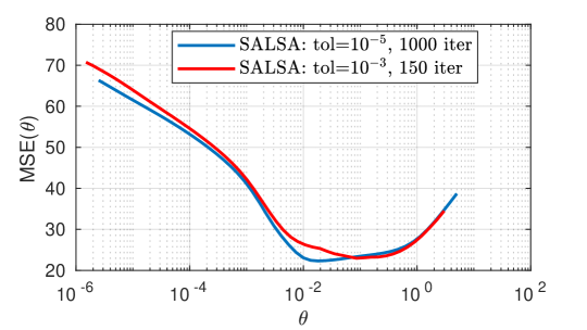
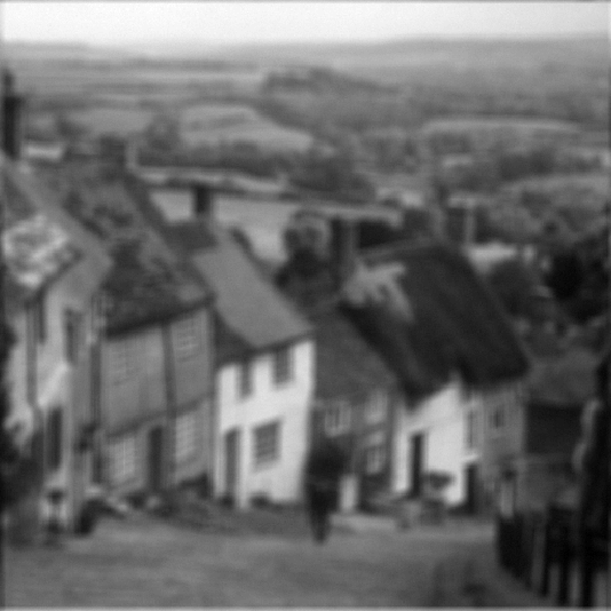
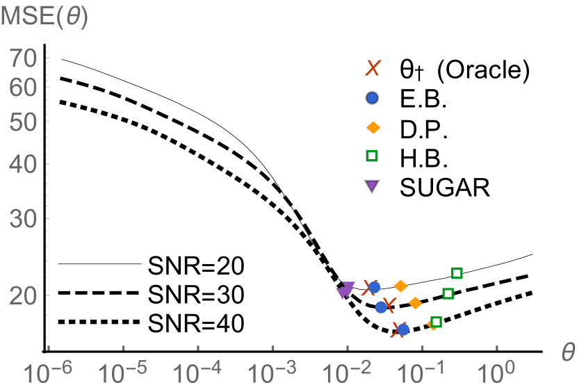
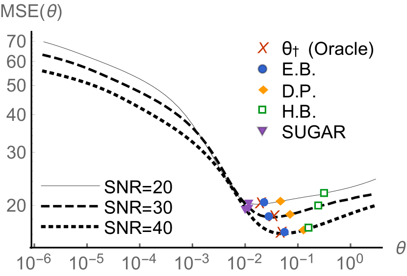
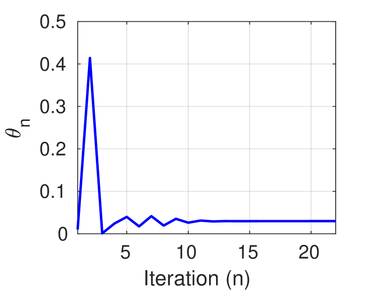
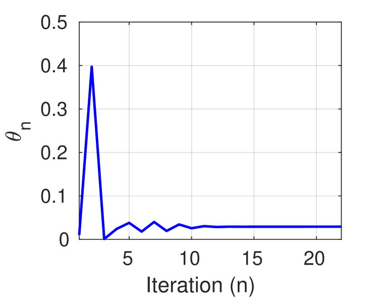
For illustration, Figure 5 shows the results obtained for two of the test images (man and goldhill) using the proposed method. The displayed images correspond to the setup. In Figure 6 we compare the estimates obtained by using each of the considered methods. In this case we display a close-up on man and goldhill selecting a region that contains fine details and sharp edges. In Figure 7 and Figure 8 we provide further details for the same two images, showing a plot of the obtained with each method and the evolution of the iterates for the empirical Bayesian method.


(a) Original

(b) Degraded


(c) EB


(d) HB


(e) DP


(f) SUGAR
(a) man
(b) goldhill
(a) man
(b) goldhill
Observe in Figure 7 that the proposed empirical Bayesian algorithm yields close-to-optimal results, both for high and low values. The method based on the discrepancy principle and the hierarchical Bayesian method overestimate the amount of regularisation required. Conversely, underestimates (this can also be observed in the recovered image in Figure 6 (f), where the MAP estimate presents some ringing artefacts due to high-frequency noise amplification); this is in agreement with the results reported in [45].
Table 1 reports the average values and average computing times obtained for each method. We can see that the proposed method performs close to the oracle performance, generally outperforming the other approaches from the state of the art with very competitive computing times. In particular, observe that the proposed method performs remarkably for all values. At high values () discrepancy principle and joint MAP [53] perform similarly, whereas for low values () discrepancy principle outperforms joint MAP. Also, performs well for low , but fails to find good values of when the is higher. This might be due to the fact that minimises a surrogate of the that works well for denoising but degrades in problems that are ill-posed or ill-conditioned. We emphasise at this point that the exact computing times of each algorithm depend on the specific stopping criteria and implementation details, so rather than claiming that one method is faster than the others, what we wish to illustrate is that the computing times are all within the same order of magnitude, with being moderately slower for this particular experiment. As we mentioned before, if we had selected a tolerance of to stop our algorithm, the computing times would have increased with almost negligible changes in the . Also note that we compute the optimal for the discrepancy principle method by continuation, but one could also use a different proximal splitting strategy (see [24] for instance).
| Method | =20 | =30 | =40 | |||
|---|---|---|---|---|---|---|
| Time | Time | Time | ||||
| 23.29 | 21.39 | 19.06 | ||||
| E.B. | 23.50 | 0.84 | 21.45 | 0.85 | 19.24 | 0.85 |
| D.P. | 23.73 | 0.70 | 21.87 | 1.52 | 19.78 | 3.92 |
| H.B. | 25.07 | 0.58 | 22.84 | 1.27 | 19.84 | 3.27 |
| 23.66 | 3.64 | 23.16 | 5.00 | 23.05 | 5.63 | |
(a)
![[Uncaptioned image]](/html/1911.11709/assets/x36.png)
(b)
4.2.2 Deconvolution with Total Variation prior and unknown noise variance
In this section we consider the same experiment as in Section 4.2.1, but we now suppose that the noise variance is unknown and explain how to modify our methodology to estimate this quantity jointly with by marginal MLE. This is beyond the scope of the theoretical results we present in our companion paper [27]. However, we believe that the theory could be generalised to provide some (albeit weaker) guarantees for this case and other blind and semi-blind problems, and this is an important perspective for future work.
More precisely, we can use the proposed scheme to compute
| (35) |
where define a minimum and maximum admissible variance values. To obtain an estimate of in Algorithm 1 we differentiate w.r.t. and obtain
| (36) |
We summarise the resulting scheme for jointly estimating and in Algorithm 4 below.
One of the complications that stems from working with an unknown noise variance is that the Lipschitz constant is unknown. This is a problem because affects the maximum step-size that we can use in the Markov Kernels while ensuring convergence; is usually also used to set . To overcome this, we propose to initialise the algorithm by assuming the worst case scenario, i.e. , which will lead to the largest , and in turn lead to the smallest possible step-size and a small . Since this value is usually very conservative, one can run some iterations of the algorithm until the value of begins to stabilise, then refine to update the algorithm parameters and , and continue iterations with those updated values. Here we adopt this approach and run the algorithm in three stages, where we update and at the end of each stage by using the estimates of available at that point to refine . In accordance with the guidelines provided in Section 3.3.1, we set with and . We have set and by assuming prior knowledge that the SNR is between dB and dB, but other values could be used without significantly impacting results. In each stage we use warm-up iterations, set , , , , , and for any . At each stage, we use the same stopping criteria as in Section 4.2.1, with a tolerance of both for and (the algorithm progresses to the next stage (or is stopped) when both iterates meet the criteria).

(a) Degraded

(b) EB with known

(c) EB with unknown
For illustration, Figure 9 shows the results obtained with Algorithm 4 for the man test image. For comparison, we also show the results of Section 4.2.1 obtained by using the true value of . The displayed images correspond to the setup. Observe there is very little difference between the recovered image using the true value of and the marginal MLE estimate obtained with Algorithm 4.
| Method | =20 | =30 | =40 | |||
|---|---|---|---|---|---|---|
| Time (min) | Time (min) | Time (min) | ||||
| 23.29 | 21.39 | 19.06 | ||||
| E.B. with known | 23.50 | 0.84 | 21.45 | 0.85 | 19.24 | 0.85 |
| E.B. with unknown | 23.53 | 1.02 | 21.52 | 1.35 | 19.27 | 1.77 |
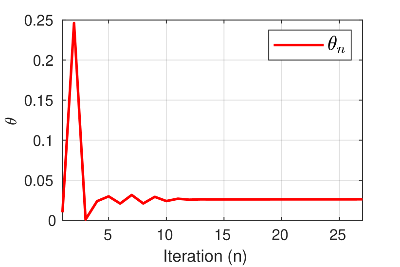
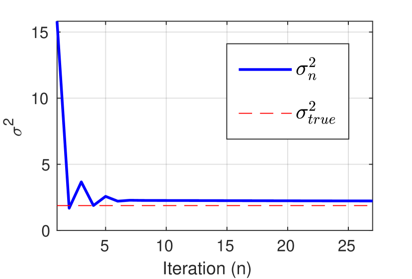
Table 2 presents a detailed comparison of the results obtained with Algorithm 4. Again, observe that the quality of the restored images obtained with the marginal MLE estimate is comparable to that of the images obtained with the true value of , with a moderate overhead in the computing times when the three-stage approach is used. We conclude by presenting in Figure 10 the evolution of the iterates and for the last stage of the algorithm (the first two stages are discarded). Observe that the algorithm converges very quickly, similarly to the case when is known.
4.2.3 Wavelet deconvolution with synthesis prior
We now consider image deblurring under a wavelet synthesis formulation, where we assume that represents the unknown image in an redundant 4-level Haar wavelet representation , with dimension coefficients. We assume a Laplace prior on the elements of with unknown parameter . Accordingly, the posterior is of the form (6) with , . To obtain solutions we map to pixel domain by computing .
To compute we use Algorithm 1. The algorithm parameters are chosen following the recommendations provided in Section 3.3.1; we do not consider any warm-up iterations, and set , , for any , , , with and . We use the same stopping criteria as in the previous experiment and we consider two different tolerance levels: i) we stop the algorithm when the relative change is smaller than , and ii) when the relative change is smaller than . We set to have burn-in iterations and compute using (16). To compute the MAP estimate we use SALSA with the following parameters: , outeriters = , tol = and mu = .
(a) Degraded

(b) EB
(c) Degraded
(d) EB
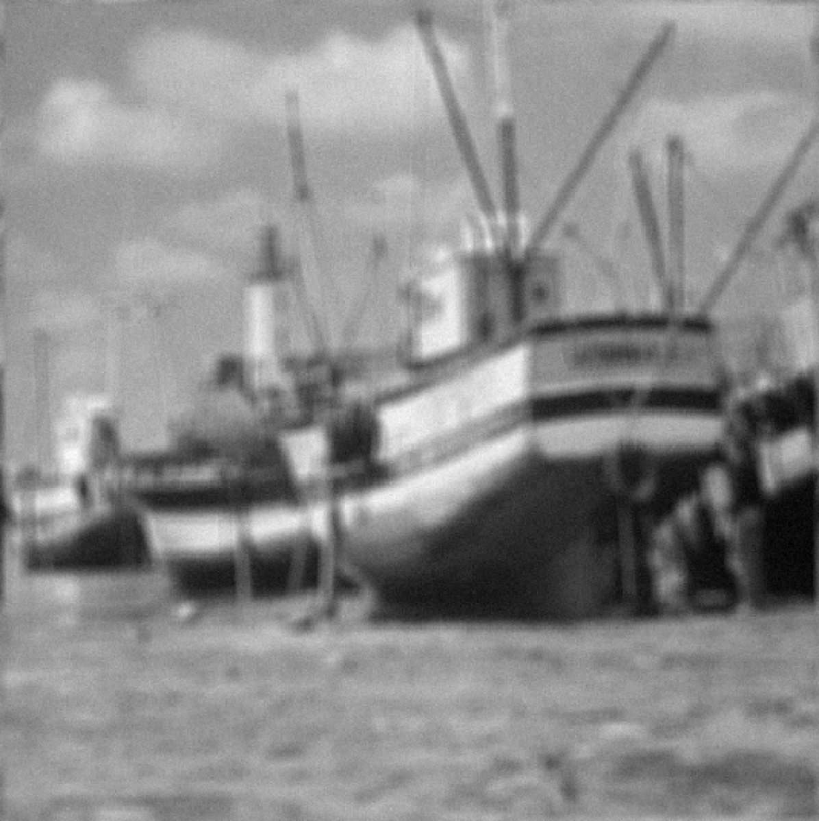
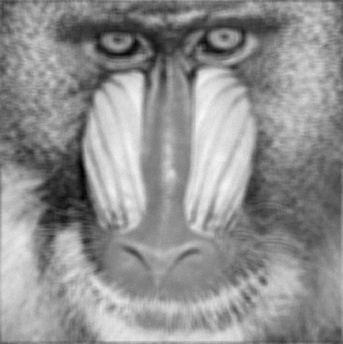
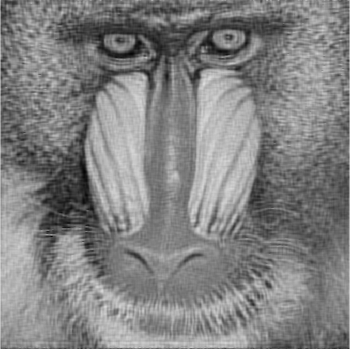
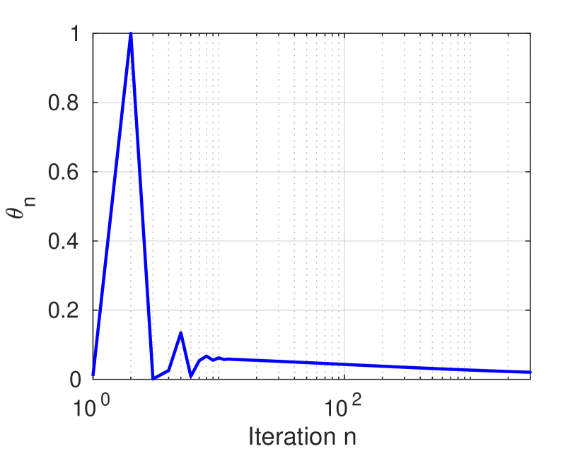
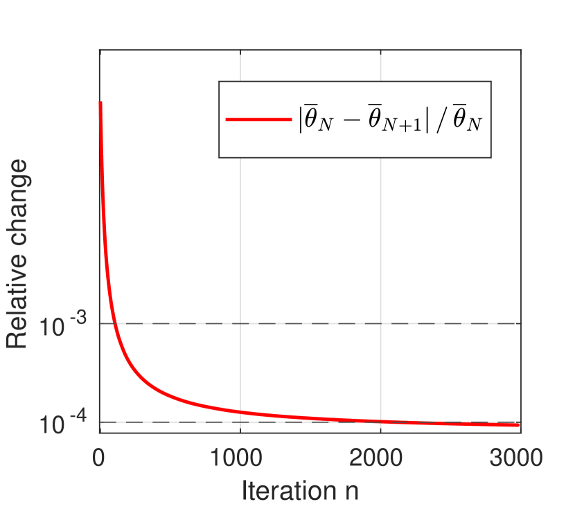
In Figure 11 we show the results obtained for two of the test images (boat and mandrill) using the proposed method. The displayed images correspond to the setup. In Figure 12 we provide further details for the boat image, showing the evolution of the iterates and the relative differences on its running average value throughout iterations.
(a)
(b)
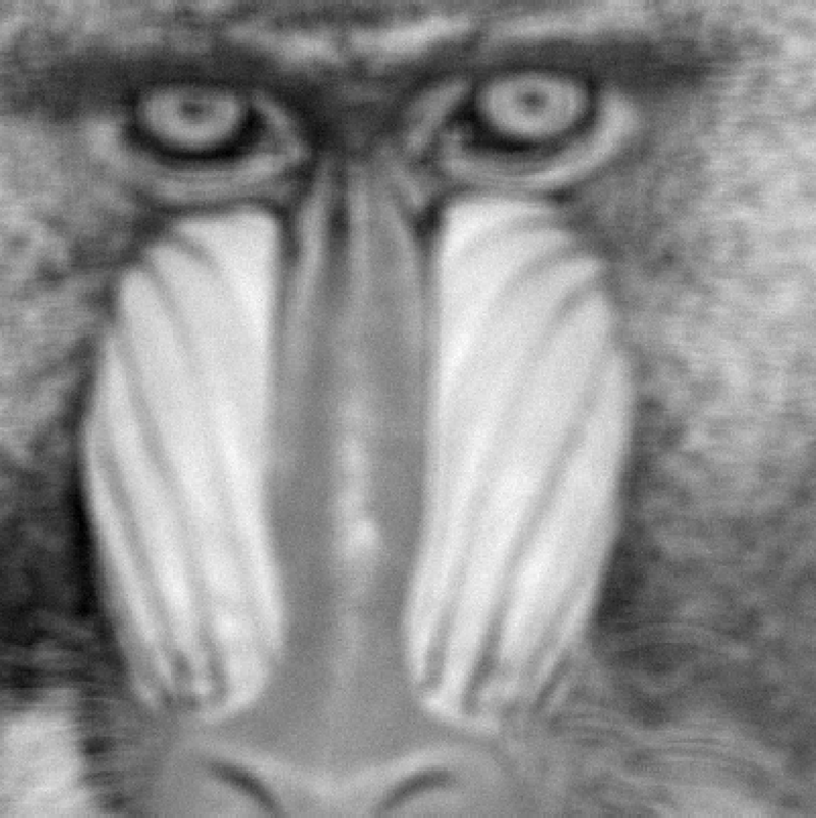
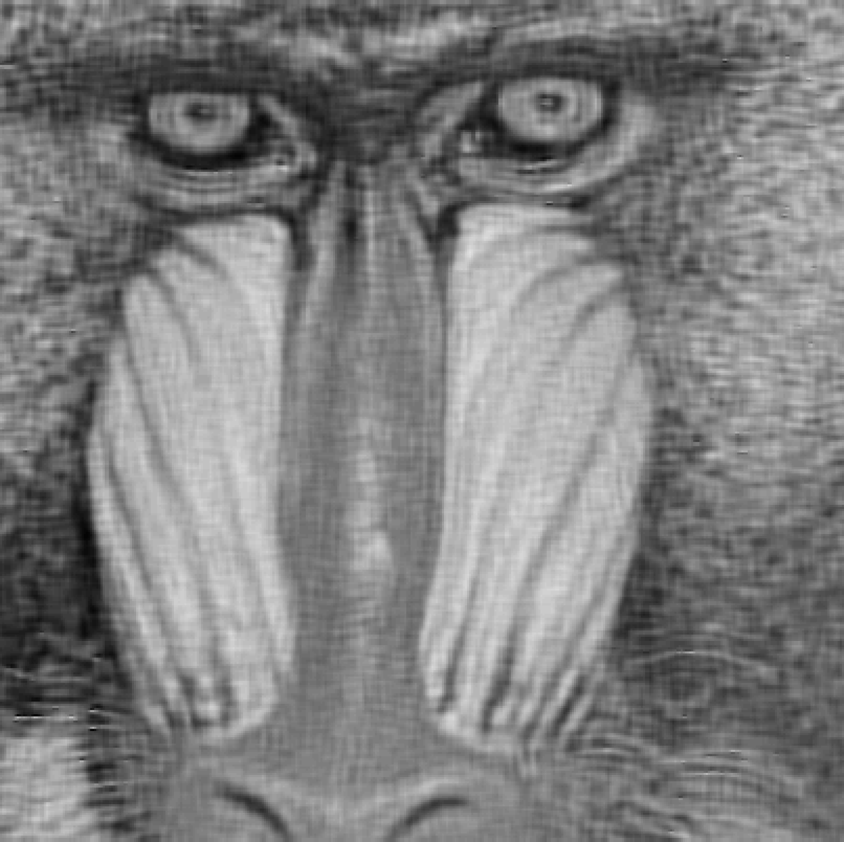
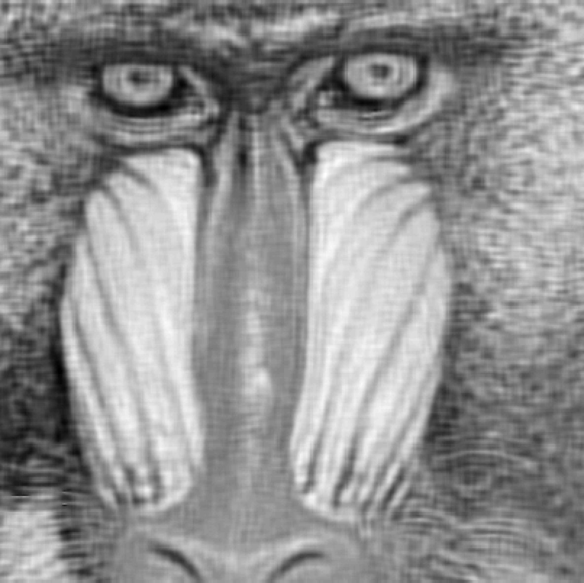
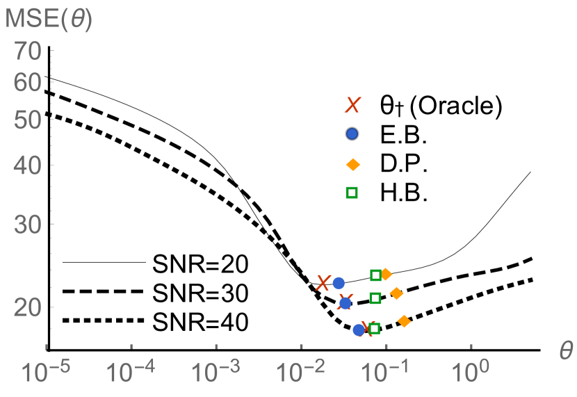
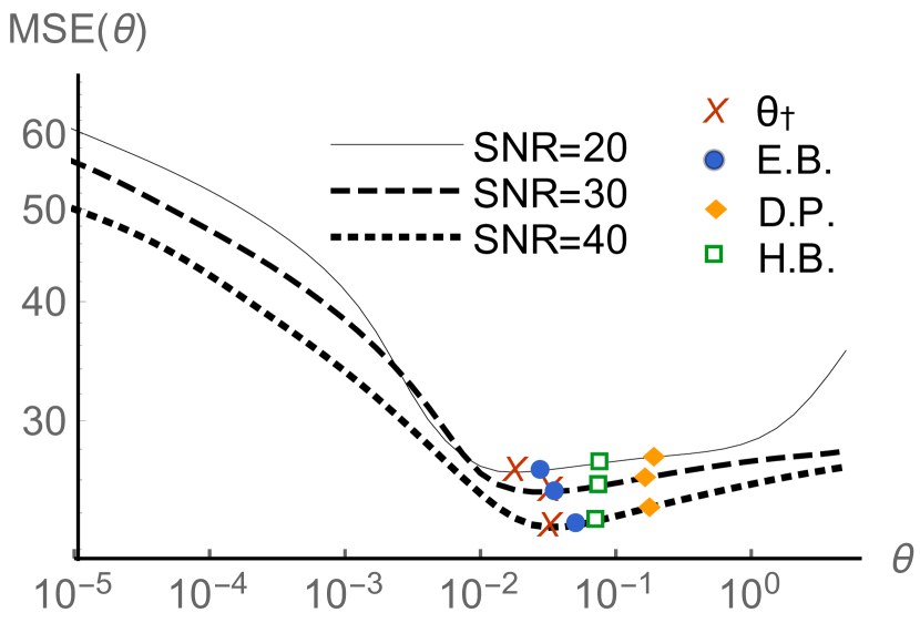
In Figure 13 we compare the results obtained by using each of the considered methods, showing a close-up on an image region that contains fine details and sharp edges. Figure 14 shows a plot of the obtained with each method for the same two test images.


(a) Original

(b) Degraded

(c) EB tol

(d) EB tol


(e) HB


(f) DP
(a) boat
(b) mandrill
Table 3 shows the average values and average computing times obtained for each method. We observe once again that the empirical Bayesian method achieves the best results for all values and is very close to the oracle performance. Reducing the tolerance leads to a small improvement in , at the expense of a higher computing time. The discrepancy principle consistently overestimates the parameter leading to over-smoothed solutions.
| Method | =20 | =30 | =40 | |||
|---|---|---|---|---|---|---|
| Time | Time | Time | ||||
| 24.23 | 22.70 | 20.56 | ||||
| E.B. | 24.40 | 4.48 | 22.80 | 3.59 | 20.70 | 2.44 |
| E.B. | 24.70 | 0.36 | 22.90 | 0.25 | 20.80 | 0.09 |
| D.P. | 25.09 | 13.93 | 23.57 | 28.64 | 21.38 | 61.03 |
| H.B. | 25.01 | 11.61 | 23.23 | 23.87 | 20.89 | 50.86 |
(a)
![[Uncaptioned image]](/html/1911.11709/assets/x62.png)
(b)
For high values, both Bayesian methods attain similar values of , but the proposed empirical Bayes methodology is five times faster. We want to point out that these general conclusions depend a lot on the parameters used for the solver of the MAP estimation problem (in this case SALSA [1]). We included a detailed analysis of this in Appendix C.
4.3 Hyperspectral Unmixing with -SUnSAL
Hyperspectral sensors acquire hundreds of narrow band spectral images in different frequency bands. These images are collected in a three-dimensional hyperspectral data cube for processing and analysis. Although the spectral resolution is high, the spatial resolution is usually low, leading to the existence of “mixed” spectra in the acquired image pixels [38]. Hyperspectral unmixing is a source separation problem that aims at decomposing each mixed pixel into its constituent spectra (the so-called end-members) and their corresponding fractional abundances or proportions. This is normally done under the assumption of a linear mixing model [65]. In particular, linear unmixing techniques assume the availability of a library of spectral signatures and use a model , where is the hyperspectral image with frequency channels and pixels; is the fractional abundance matrix compatible with the library containing the pure spectral signatures for different materials; and is a Gaussian random variables with zero mean and covariance matrix and . In [38], the unmixing problem is solved by using the regulariser given for any by
| (37) |
which is associated with a two dimensional regularisation parameter . controls the spatial cohesion of the objects, and enforces sparsity on . In this experiment, is the vectorial isotropic total variation pseudo-norm given for any by
| (38) |
where for any , denotes the -th image pixel and its vertical and horizontal neighbour pixels.
Although this regulariser is not separable and we would therefore have to use Algorithm 3 with two MCMC chains, we can use a pseudo-likelihood approximation estimate using a single MCMC chain together with the expression of for the homogeneous case. In this way we can achieve highly competitive computing times as well as compare our results with the hierarchical Bayesian method from [53], which we would otherwise not be able to apply to this problem.
More precisely, we consider and . Although and are not acting on independent subsets of , we have empirically observed that this provides a good approximation and delivers excellent results.
We consider the experiment A-Simulated Data Sets case 1) Simulated Data Cube 1 presented in [38, Section 4], particularly the case where is a white Gaussian noise. In this experiment a synthetic hyperspectral image is generated by using five randomly selected spectral signatures. The image has pixels and frequency bands per pixel. For full details see [38]. We follow the exact same procedure as presented there, except for a modification in the spectral signature dictionary . In [38] they consider a dictionary , which is a library generated from a random selection of 240 materials from the USGS library777Available online: http://speclab.cr.usgs.gov/spectral.lib06. Here we consider a simplified version where we only select random materials, thus having . Out of these 12 materials, only 5 are present in the synthetic image. The synthetic fractional abundances are displayed in the first row of Figure 15 (only the 5 present end-members are shown)
We use the proposed algorithm to estimate and for this setup using Algorithm 2 under three different noise levels: we consider a of , and . For comparison, we also report the results obtained with the joint MAP method from [53] and by using the oracle value that maximises the estimation signal-to-reconstruction-error (SRE) given by .
We evaluated the proximal operator of using SUnSAL solver from [38] with 20 iterations. We address the positivity constraint separately by using its Moreau-Yosida envelope, leading to the additional term where is the projection operator onto , and is the same smoothing parameter used for the other proximal operators.
To speed up the convergence, we use a gradient preconditioning technique explained in Section B.5. Since we use the preconditioned gradient of instead of the gradient of , the Lipschitz constant becomes . The algorithm parameters are chosen following the recommendations provided in Section 3.3.1; we set , , we initialised using the pseudo-inverse of and projecting on the space of positive matrices. In addition, we perform warm-up iterations and set for any , and .
Special care was taken when setting and due to the preconditioning. We set for any and , where is the largest eigenvalue of . We run the algorithm for 50 iterations and compute as defined in (16) with set to have burn-in iterations.
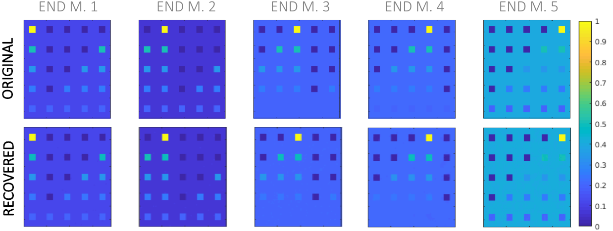
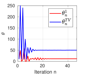
In Figure 15 we display the MAP recovery of the synthetic fractional abundances using the estimated values of and with the SUnSAL solver for =30 . Figure 16 shows the evolution of the iterates and and the relative change in the running averages throughout iterations for =30 . Observe the excellent convergence properties of the proposed scheme, which stabilises in as little as iterations.

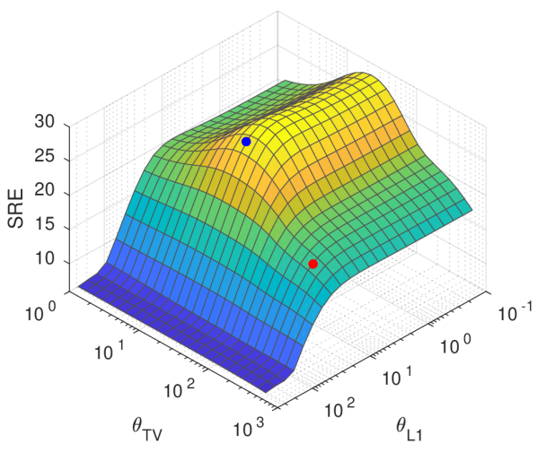
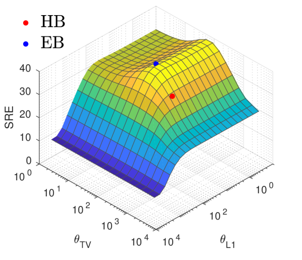
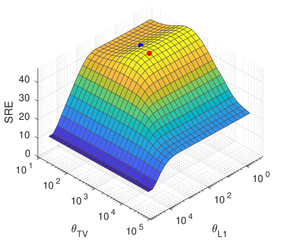
The obtained results are reported in Table 4 and summarised in Figure 17, which shows the signal to reconstruction error (SRE) surfaces for different values of the regularisation parameters. Observe that the empirical Bayesian method yields good results for all
| Method | =20 | =30 | =40 | ||||
| Stop criteria | SRE | Time (s) | SRE | Time (s) | SRE | Time (s) | |
| (Oracle) | – | 29.38 | – | 38.61 | – | 47.64 | – |
| E.B. | 50 iters. | 27.46 | 36 | 38.42 | 37 | 45.68 | 42 |
| H.B. [53] | 15 iters. | 18.33 | 76 | 31.72 | 77 | 47.36 | 76 |
(a) =20
(b) =30
(c) =40
values, and clearly outperforms the hierarchical Bayesian method for low values. For high values the hierarchical method achieved slightly better results. As discussed in Section 3.4, we believe that this is due to the fact that, at high values, the likelihood dominates the posterior and mitigates errors related to the misspecification of the prior. More precisely, if the hyperprior that we set on assigns a high weight to values of that lead to bad models, i.e. a misspecified prior , the impact of this misspecification on the recovered estimates depends on the degree of concentration of the likelihood. At high SNR, the likelihood dominates the posterior thus concealing the possible prior misspecification and leading to good results. Conversely, at low values, the performance of the hierarchical model is degraded by model misspecification.
Also note in Table 4 that the computing times for the empirical Bayesian method are approximately two times faster than the ones for the hierarchical method.
4.4 Denoising with a total generalised variation prior
In this last experiment, we apply the proposed methodology to a challenging problem that is beyond the scope of the considered class of models and our theoretical guarantees. We consider an image denoising problem where with and where we use the following prior
where and where is a second-order generalisation of the conventional total variation regulariser, given, for any and , by
| (39) |
where is the discrete image-gradient operator that computes the first-order vertical and horizontal pixel differences, and computes the Jacobian matrix of the image-gradient vector field to capture second-order information (i.e., is a discrete image-Hessian operator) [25]. This generalisation was first considered in [21] and further studied in [14] as a means of incorporating second-order derivative information to eliminate the common staircasing artifacts associated with the conventional regulariser.
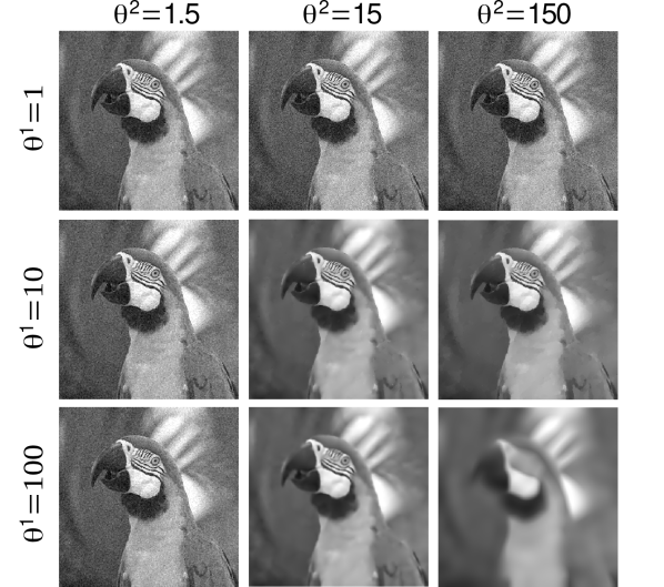
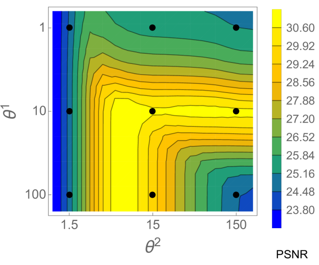
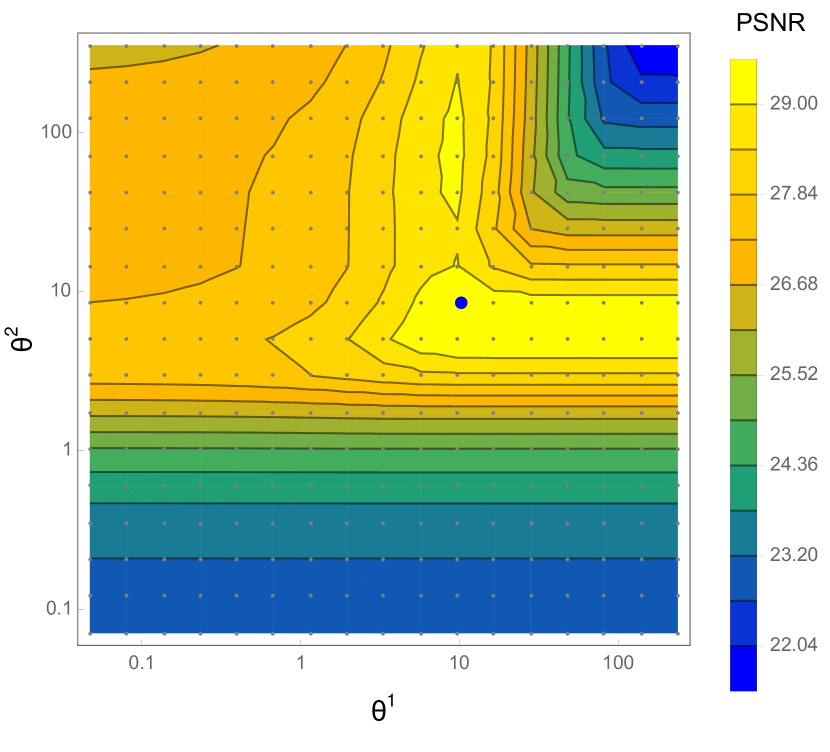
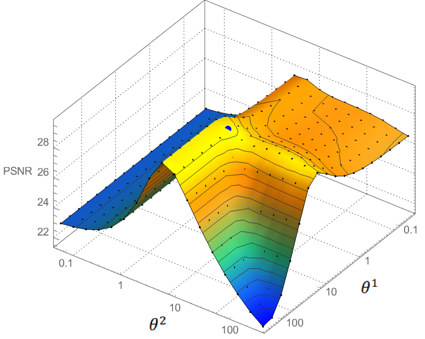
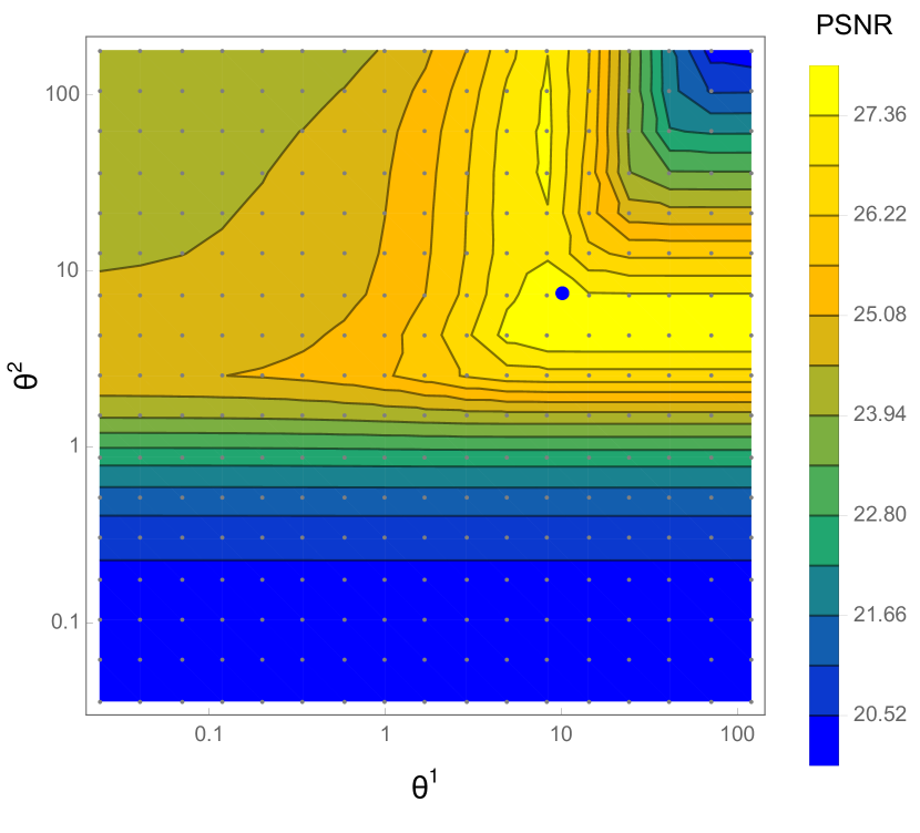
A main difficulty associated with using the regulariser is the need to correctly set the parameters and , which control the strength as well as the characteristics of the regularisation enforced (as explained in [25], the regularisation behaves like the standard regularisation for large values, whereas for small values it behaves like the -Frobenius norm of the discrete image-Hessian). Figure 18 below illustrates the dramatic effect that these two parameters have on the quality of the recovered MAP estimate. Observe the strong coupling between and , which makes setting their values particularly challenging.
However, this prior is not in the exponential family because and play a role in the definition of the statistic . Therefore, our methodology and theory do not directly apply. Also note that the additional regularisation with is necessary to guarantee that is proper, which is potentially important in order to apply the proposed methodology with two Markov chains (otherwise the auxiliary chain targeting would not be ergodic - two chains are required because (39) is not separable and homogeneous). We use .
In order to apply the proposed methodology to the estimation of and we use an approximation of the gradient . More precisely, we express as follows for any and
with
and approximate the partial derivatives and by
This approximation of the gradient, which arises from omitting the terms
and
in the calculation of the partial derivatives and , introduces an additional bias in the stochastic gradients driving Algorithm 3888A rigorous analysis of this bias should also consider the points where is not differentiable w.r.t. and . This can be achieved by using similar techniques to [26].. However, the numerical experiments reported below suggest that the algorithm is robust to this additional bias, in the sense that we empirically observe good convergence to useful estimates of and .
In our experiments, we implement Algorithm 3 with this approximate gradient and follow the recommendations provided in Section 3.3.1 to set the algorithm parameters; we perform warm-up iterations and set , , for any , and , and we set with and . To stop the algorithm we consider three different cases: we stop the algorithm i) after fixed iterations ii) when the relative change in is and iii) . Again, we compute using (16), setting to have burn-in iterations.
We also considered a thinning of iterations in the chain associated with the prior as its samples were roughly times more correlated than those coming from the chain targeting the posterior (i.e., we discard every samples as explained in Section B.3). To compute the norm and proximal operator, we use the iterative primal-dual algorithm [25].
Applying Algorithm 3 to the entire image is too computationally expensive because of the complexity associated with evaluating the proximal operator of the TGV regulariser. Therefore, in this experiment we estimate from a representative patch of size pixels, and then use the estimated and values to compute the MAP estimate of the entire image999For homogeneous regularisers, is asymptotically independent of the dimension of when is large, suggesting that it is possible to estimate its value from a representative image patch. Our empirical results suggest that this might hold for other models as well.. We consider the same ten test images used in Section 4.2 and we set the noise variance , such that the signal-to-noise-ratio () is , , or . For each image and noise level, we first obtain an estimate for and and then use them to compute the MAP estimator (given by (7)) using the same solver [25] we use for the proximal operator. We measure estimation performance by computing the peak-signal-to-noise-ratio (PSNR) given by . All the plots shown in Figure 20, Figure 21 and Figure 24 were computed with the entire image.
Table 5 below summarises the average PSNR values and average computing times obtained for each SNR value for the three different stopping criteria. We observe that the proposed empirical Bayesian method achieves very good results for all SNR values and is very close to the oracle performance. Crucially, the stopping criteria has a strong impact on the computing times but not on the resulting PSNR values. Therefore, although convergence can take close to one hour with a strict convergence criterion, good results can be obtained in the order of a minute by using a weaker convergence criterion.
| Method | =8 | =12 | =20 | |||
|---|---|---|---|---|---|---|
| P | Time | PSNR | Time | PSNR | Time (min) | |
| (Oracle) | 27.80 2.35 | 30.21 2.12 | 35.60 1.77 | |||
| 2000 iter E.B. | 27.11 2.81 | 131.10 | 29.69 2.33 | 96.41 | 35.48 1.81 | 95.06 |
| E.B. | 27.09 2.84 | 24.61 | 29.72 2.33 | 23.27 | 35.47 1.81 | 44.70 |
| E.B. | 27.00 2.96 | 3.04 | 29.50 2.71 | 2.18 | 35.57 1.79 | 5.03 |
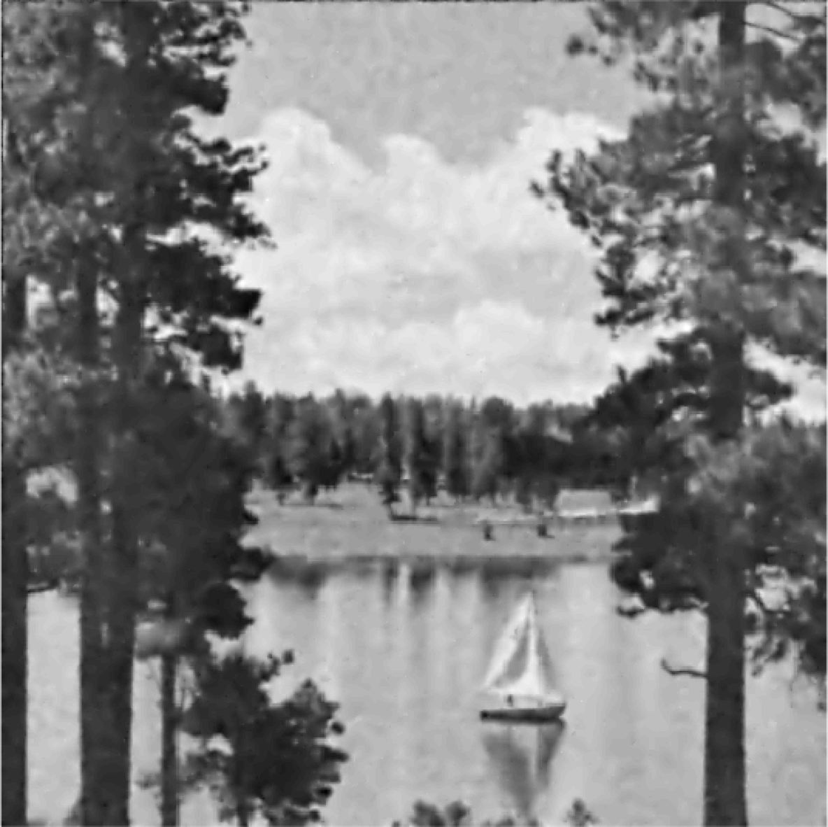
For illustration, Figure 19 depicts the original image, the noisy observation and the recovered MAP estimates for the boat and lake test images with .


(a) Original


(b) Degraded

(c) Empirical Bayes
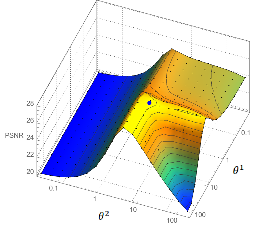
More interestingly, Figure 20 and Figure 21 show the landscape of the as a function of and for the two test images, with the obtained solutions highlighted as a blue dot. Observe that the estimated solutions are extremely close to the optimal ones, which is remarkable given the difficulty of the problem and the fact that solutions are derived directly from statistical inference principles, without any form of ground truth.
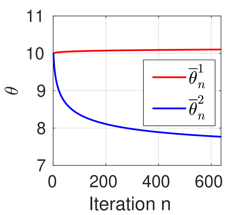
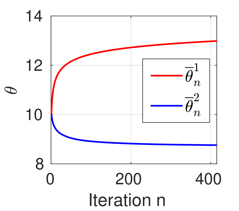
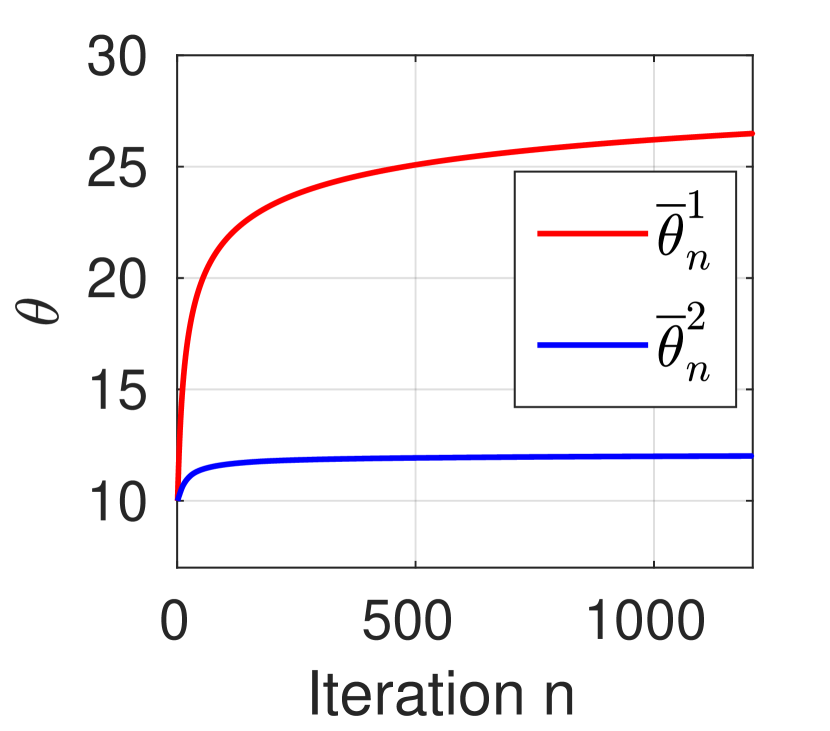
Following on from this, Figure 22 and Figure 23 show, respectively, the evolution of the iterates and the relative change in the estimated values of and , for the lake test image, and for , , and . Observe that the algorithm converges quickly and can deliver a useful solution in approximately iterations if the weaker convergence criterion is used, or in approximately iterations if one uses a stricter convergence criterion.
(a) 8
(b) 12
(c) 20
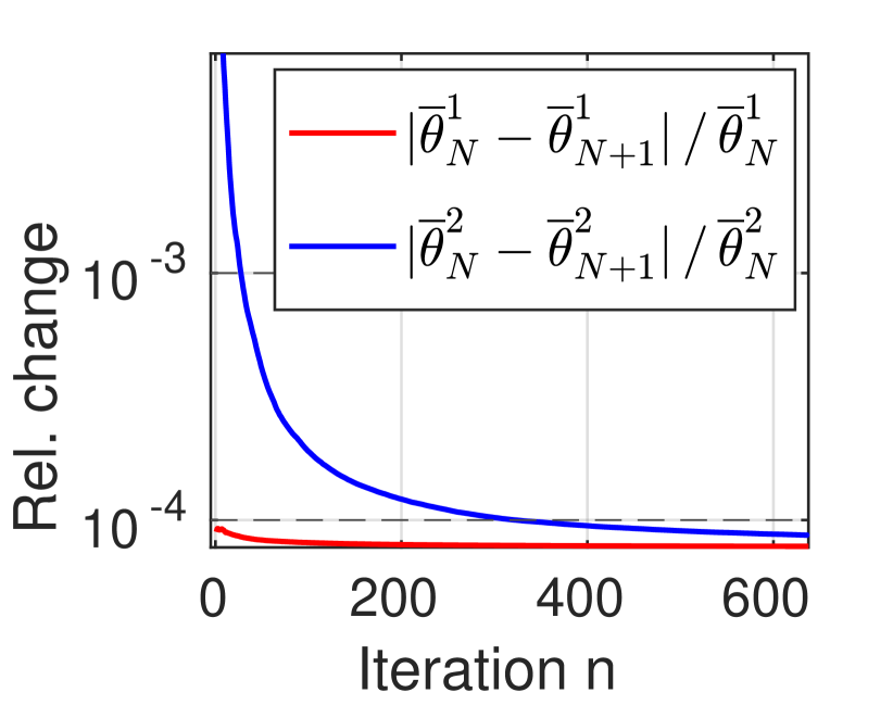
(a) 8
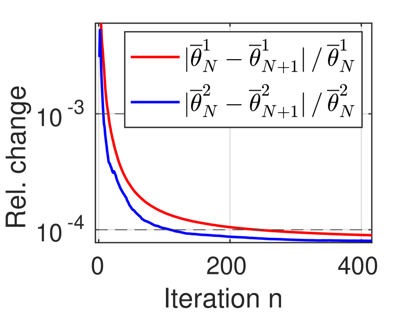
(b) 12
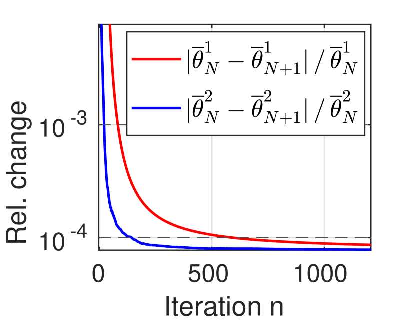
(c) 20
Lastly, Figure 24 below explores the robustness to different initialisations by showing the evolution of the iterates on the landscape of PSNR values for the flintstones image with . We consider three different initialisations, highlighted in colours red, green, and blue, and observe that in the three cases the algorithm quickly converges to values for the parameters and that are close-to-optimal in terms of the resulting PSNR. However, the algorithm is not fully robust to bad initialisation because of the non-convexity and the approximations involved. For example, initialising the algorithm in the corner of the PSNR landscape (e.g., ) does not lead to a satisfactory solution, indicating that a careful initialisation is required. Alternatively, one could also initialise the algorithm by performing a certain number of updates on with fixed to a small value - e.g. - to keep the model close to the conventional total variation regulariser, and then update both with until the convergence criterion is satisfied.
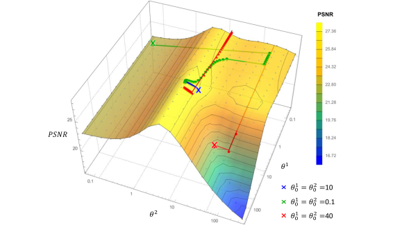
To conclude, we note that there are several other generalisations of the total variation regularisation (see [14]). We have chosen to perform our experiments with (39) because of the availability of the efficient MATLAB implementation [25]. However, we expect that Algorithm 3 will also perform well for other generalisations of the total variation norm, particularly the second-order generalisation proposed in [14] that is very similar to (39).
5 Conclusions
This paper considered the automatic selection of regularisation parameters in imaging inverse problems, with a particular focus on problems that are convex w.r.t. the unknown image and possibly non-smooth, and which would be typically solved by maximum-a-posteriori estimation by using modern proximal optimisation techniques. We adopted an empirical Bayesian approach and proposed a computational method to efficiently and accurately estimate regularisation parameters by maximum marginal likelihood estimation. The considered marginal likelihood function is computationally intractable and we proposed to address this difficulty by using a stochastic proximal gradient optimisation algorithm that is driven by two proximal MCMC samplers, and which tightly combines the strengths of modern high-dimensional optimisation and Monte Carlo sampling techniques. Because the proposed method uses the same basic operators as proximal optimisation algorithms, namely gradient and proximal operators, it is straightforward to apply to problems that are currently solved by proximal optimisation. Moreover, we provided a detailed theoretical analysis of the proposed methodology, including easily verifiable conditions for convergence. In addition to being highly computational efficient and having strong theoretical underpinning, the proposed methodology is very general and can be used to simultaneously estimate multiple regularisation parameters, unlike some alternative approaches from the literature that can only handle a single or scalar parameter.
We demonstrated the methodology with a range of imaging problems and models. We first considered image denoising and non-blind deblurring problems involving scalar regularisation parameters and showed that the method achieved close-to-optimal performance in terms of MSE and outperformed alternative approaches from the literature. We then successfully applied the method to two challenging problems involving bivariate regularisation parameters: a sparse hyperspectral unmixing problem with a total-variation plus sparsity prior, and a challenging denoising problem using a second-order total generalised variation regulariser. Again, the method delivered close-to-optimal results, as measured by estimation MSE.
Future work will focus on relaxing the convexity assumptions to provide theoretical convergence guarantees for non-convex problems, and on improving computational efficiency by using the recently proposed accelerated proximal Markov kernels [70]. The application of the proposed methodology to challenging problems arising in medical and astronomical imaging is currently under investigation. Another important perspective for future work is to extend this methodology to semi-blind and blind imaging problems, as well as to problems involving space-varying regularisation parameters [42].
6 Acknowledgements
We are grateful to Dr. Charles Deledalle for providing us with a SUGAR implementation for an ADMM solver available at https://github.com/deledalle/sugar/blob/master/solvers/admm.m. AD acknowledges financial support from Polish National Science Center grant: NCN UMO-2018/31/B/ST1/00253. The work of MP is supported by UKRI/EPSRC under grant EP/T007346/1.
References
- [1] Manya V Afonso, José M Bioucas-Dias, and Mário AT Figueiredo. Fast image recovery using variable splitting and constrained optimization. IEEE Transactions on Image Processing, 19(9):2345–2356, 2010.
- [2] Mariana SC Almeida and Mário AT Figueiredo. Parameter estimation for blind and non-blind deblurring using residual whiteness measures. IEEE Transactions on Image Processing, 22(7):2751–2763, 2013.
- [3] Simon Arridge, Peter Maass, Ozan Öktem, and Carola-Bibiane Schönlieb. Solving inverse problems using data-driven models. Acta Numerica, 28:1–174, 2019.
- [4] Yves F Atchadé. An adaptive version for the Metropolis adjusted Langevin algorithm with a truncated drift. Methodology and Computing in applied Probability, 8(2):235–254, 2006.
- [5] Yves F. Atchadé. A computational framework for empirical Bayes inference. Statistics and Computing, 21(4):463–473, 2011.
- [6] Yves F Atchadé, Gersende Fort, and Eric Moulines. On perturbed proximal gradient algorithms. J. Mach. Learn. Res, 18(1):310–342, 2017.
- [7] S Derin Babacan, Rafael Molina, and Aggelos K Katsaggelos. Parameter estimation in TV image restoration using variational distribution approximation. IEEE transactions on image processing, 17(3):326–339, 2008.
- [8] S Derin Babacan, Rafael Molina, and Aggelos K Katsaggelos. Variational Bayesian super resolution. IEEE Transactions on Image Processing, 20(4):984–999, 2011.
- [9] Francis R. Bach and Eric Moulines. Non-asymptotic analysis of stochastic approximation algorithms for machine learning. In Advances in Neural Information Processing Systems 24: 25th Annual Conference on Neural Information Processing Systems 2011. Proceedings of a meeting held 12-14 December 2011, Granada, Spain, pages 451–459, 2011.
- [10] Heinz H. Bauschke and Patrick L. Combettes. Convex analysis and monotone operator theory in Hilbert spaces. CMS Books in Mathematics/Ouvrages de Mathématiques de la SMC. Springer, Cham, second edition, 2017. With a foreword by Hédy Attouch.
- [11] Federico Benvenuto and Cristina Campi. A discrepancy principle for the landweber iteration based on risk minimization. Applied Mathematics Letters, 96:1 – 6, 2019.
- [12] Sergey Bobkov and Mokshay Madiman. Concentration of the information in data with log-concave distributions. Annals of Probability, 39(4):1528–1543, 2011.
- [13] Léon Bottou. Stochastic gradient descent tricks. In Neural networks: Tricks of the trade, pages 421–436. Springer, 2012.
- [14] Kristian Bredies, Karl Kunisch, and Thomas Pock. Total generalized variation. SIAM Journal on Imaging Sciences, 3(3):492–526, 2010.
- [15] Luca Calatroni, Chung Cao, Juan Carlos De Los Reyes, Carola-Bibiane Schönlieb, and Tuomo Valkonen. Bilevel approaches for learning of variational imaging models. Variational Methods: In Imaging and Geometric Control, 18(252):2, 2017.
- [16] D Calvetti, S Morigi, L Reichel, and F Sgallari. Tikhonov regularization and the l-curve for large discrete ill-posed problems. Journal of computational and applied mathematics, 123(1-2):423–446, 2000.
- [17] Daniela Calvetti, Monica Pragliola, Erkki Somersalo, and Alexander Strang. Sparse reconstructions from few noisy data: analysis of hierarchical bayesian models with generalized gamma hyperpriors. Inverse Problems, 36(2):025010, 2020.
- [18] Daniela Calvetti and Erkki Somersalo. Hypermodels in the bayesian imaging framework. Inverse Problems, 24(3):034013, 2008.
- [19] Daniela Calvetti, Erkki Somersalo, and A Strang. Hierachical bayesian models and sparsity: 2-magic. Inverse Problems, 35(3):035003, 2019.
- [20] Bradley P. Carlin and Thomas A. Louis. Empirical Bayes: past, present and future. J. Amer. Statist. Assoc., 95(452):1286–1289, 2000.
- [21] Antonin Chambolle and P.-L. Lions. Image recovery via total variation minimization and related problems. Numerische Mathematik, 76:167–188, 1997.
- [22] Antonin Chambolle and Thomas Pock. A first-order primal-dual algorithm for convex problems with applications to imaging. Journal of mathematical imaging and vision, 40(1):120–145, 2011.
- [23] Antonin Chambolle and Thomas Pock. An introduction to continuous optimization for imaging. Acta Numerica, 25:161–319, 2016.
- [24] Patrick L Combettes and Jean-Christophe Pesquet. Proximal splitting methods in signal processing. In Fixed-point algorithms for inverse problems in science and engineering, pages 185–212. Springer, 2011.
- [25] Laurent Condat. Matlab code for total generalized variation denoising, 2016.
- [26] V. De Bortoli, A. Durmus, M. Pereyra, and A. F. Vidal. Efficient stochastic optimisation by unadjusted langevin monte carlo. application to maximum marginal likelihood and empirical bayesian estimation. 2019.
- [27] Valentin De Bortoli, Durmus Alain, Marcelo Pereyra, and Ana Fernandez Vidal. Maximum likelihood estimation of regularisation parameters in high-dimensional inverse problems: an empirical bayesian approach. Part II: Theoretical analysis. arXiv preprint arXiv:2008.05793, 2020.
- [28] Charles-Alban Deledalle, Samuel Vaiter, Jalal Fadili, and Gabriel Peyré. Stein Unbiased GrAdient estimator of the Risk (SUGAR) for multiple parameter selection. SIAM Journal on Imaging Sciences, 7(4):2448–2487, 2014.
- [29] Randal Douc, Eric Moulines, and David Stoffer. Nonlinear time series: Theory, methods and applications with R examples. Chapman and Hall/CRC, 2014.
- [30] Alain Durmus, Eric Moulines, and Marcelo Pereyra. Efficient Bayesian computation by proximal Markov chain Monte Carlo: when Langevin meets Moreau. SIAM Journal on Imaging Sciences, 11(1):473–506, 2018.
- [31] Yonina C Eldar. Generalized SURE for exponential families: Applications to regularization. IEEE Transactions on Signal Processing, 57(2):471–481, 2009.
- [32] Heinz Werner Engl, Martin Hanke, and Andreas Neubauer. Regularization of inverse problems, volume 375. Springer Science & Business Media, 1996.
- [33] Gersende Fort, Edouard Ollier, and Adeline Samson. Stochastic Proximal Gradient Algorithms for Penalized Mixed Models. arXiv preprint arXiv:1704.08891, 2017.
- [34] Raja Giryes, Michael Elad, and Yonina C Eldar. The projected GSURE for automatic parameter tuning in iterative shrinkage methods. Applied and Computational Harmonic Analysis, 30(3):407–422, 2011.
- [35] Gene H Golub, Michael Heath, and Grace Wahba. Generalized cross-validation as a method for choosing a good ridge parameter. Technometrics, 21(2):215–223, 1979.
- [36] Peter J Green, Krzysztof Latuszyński, Marcelo Pereyra, and Christian P Robert. Bayesian computation: a summary of the current state, and samples backwards and forwards. Statistics and Computing, 25(4):835–862, 2015.
- [37] Per Christian Hansen and Dianne Prost O’Leary. The use of the L-curve in the regularization of discrete ill-posed problems. SIAM Journal on Scientific Computing, 14(6):1487–1503, 1993.
- [38] Marian-Daniel Iordache, José M Bioucas-Dias, and Antonio Plaza. Total variation spatial regularization for sparse hyperspectral unmixing. IEEE Transactions on Geoscience and Remote Sensing, 50(11):4484–4502, 2012.
- [39] Jari Kaipio and Erkki Somersalo. Statistical and computational inverse problems, volume 160. Springer Science & Business Media, 2006.
- [40] BT Knapik, BT Szabó, AW van der Vaart, and JH van Zanten. Bayes procedures for adaptive inference in inverse problems for the white noise model. Probability Theory and Related Fields, 164(3-4):771–813, 2016.
- [41] Karl Kunisch and Thomas Pock. A bilevel optimization approach for parameter learning in variational models. SIAM Journal on Imaging Sciences, 6(2):938–983, 2013.
- [42] Alessandro Lanza, Serena Morigi, Monica Pragliola, and Fiorella Sgallari. Space-variant tv regularization for image restoration. In European Congress on Computational Methods in Applied Sciences and Engineering, pages 160–169. Springer, 2017.
- [43] Alessandro Lanza, Serena Morigi, Fiorella Sgallari, and Anthony J Yezzi. Variational image denoising based on autocorrelation whiteness. SIAM Journal on Imaging Sciences, 6(4):1931–1955, 2013.
- [44] Charles L Lawson and Richard J Hanson. Solving least squares problems, volume 15. Siam, 1995.
- [45] Felix Lucka, Katharina Proksch, Christoph Brune, Nicolai Bissantz, Martin Burger, Holger Dette, and Frank Wübbeling. Risk estimators for choosing regularization parameters in ill-posed problems-properties and limitations. Inverse Problems & Imaging, 12(5):1121–1155, 2018.
- [46] Yosra Marnissi, Yuling Zheng, Emilie Chouzenoux, and Jean-Christophe Pesquet. A Variational Bayesian Approach for Image Restoration?Application to Image Deblurring With Poisson–Gaussian Noise. IEEE Transactions on Computational Imaging, 3(4):722–737, 2017.
- [47] Rafael Molina, Aggelos K Katsaggelos, and Javier Mateos. Bayesian and regularization methods for hyperparameter estimation in image restoration. IEEE Transactions on Image Processing, 8(2):231–246, 1999.
- [48] Vishal Monga. Handbook of Convex Optimization Methods in Imaging Science. Springer, 2017.
- [49] Vladimir Alekseevich Morozov. Methods for solving incorrectly posed problems. Springer Science & Business Media, 2012.
- [50] Radford M Neal. Bayesian learning for neural networks, volume 118. Springer Science & Business Media, 2012.
- [51] Marcelo Pereyra. Proximal markov chain monte carlo algorithms. Statistics and Computing, 26(4):745–760, 2016.
- [52] Marcelo Pereyra. Revisiting Maximum-A-Posteriori Estimation in Log-Concave Models. SIAM Journal on Imaging Sciences, 12(1):650–670, 2019.
- [53] Marcelo Pereyra, José M Bioucas-Dias, and Mário AT Figueiredo. Maximum-a-posteriori estimation with unknown regularisation parameters. In Signal Processing Conference (EUSIPCO), 2015 23rd European, pages 230–234. IEEE, 2015.
- [54] Marcelo Pereyra, Nicolas Dobigeon, Hadj Batatia, and Jean-Yves Tourneret. Estimating the granularity coefficient of a Potts-Markov random field within a Markov chain Monte Carlo algorithm. IEEE Transactions on Image Processing, 22(6):2385–2397, 2013.
- [55] Marcelo Pereyra, Nicolas Dobigeon, Hadj Batatia, and Jean-Yves Tourneret. Computing the Cramer–Rao bound of Markov random field parameters: application to the Ising and the Potts models. IEEE Signal Processing Letters, 21(1):47–50, 2014.
- [56] Marcelo Pereyra, Philip Schniter, Emilie Chouzenoux, Jean-Christophe Pesquet, Jean-Yves Tourneret, Alfred O Hero, and Steve McLaughlin. A survey of stochastic simulation and optimization methods in signal processing. IEEE Journal of Selected Topics in Signal Processing, 10(2):224–241, 2016.
- [57] Jean-Christophe Pesquet, Amel Benazza-Benyahia, and Caroline Chaux. A SURE approach for digital signal/image deconvolution problems. IEEE Transactions on Signal Processing, 57(12):4616–4632, 2009.
- [58] S. Petrone, J. Rousseau, and C. Scricciolo. Bayes and empirical Bayes: do they merge? Biometrika, 101(2):285–302, 2014.
- [59] Alexander Rakhlin, Ohad Shamir, and Karthik Sridharan. Making gradient descent optimal for strongly convex stochastic optimization. arXiv preprint arXiv:1109.5647, 2011.
- [60] H. Robbins. An empirical Bayes approach to statistics. In Herbert Robbins Selected Papers, pages 41–47. Springer, 1985.
- [61] C. P. Robert and G. Casella. Monte Carlo Statistical Methods (2nd ed.). Springer-Verlag, New York, 2004.
- [62] Christian Robert. The Bayesian choice: from decision-theoretic foundations to computational implementation. Springer Science & Business Media, 2007.
- [63] J. Rousseau and B. Szabo. Asymptotic behaviour of the empirical Bayes posteriors associated to maximum marginal likelihood estimator. Ann. Statist., 45(2):833–865, 2017.
- [64] Toby Sanders, Rodrigo B Platte, and Robert D Skeel. Effective new methods for automated parameter selection in regularized inverse problems. Applied Numerical Mathematics, 2020.
- [65] Miguel Simões, José Bioucas-Dias, Luis B Almeida, and Jocelyn Chanussot. A convex formulation for hyperspectral image superresolution via subspace-based regularization. IEEE Transactions on Geoscience and Remote Sensing, 53(6):3373–3388, 2015.
- [66] Michael E Tipping. Sparse bayesian learning and the relevance vector machine. Journal of machine learning research, 1(Jun):211–244, 2001.
- [67] Michael E Tipping, Anita C Faul, et al. Fast marginal likelihood maximisation for sparse bayesian models. In AISTATS, 2003.
- [68] Cao Van Chung, JC De los Reyes, and CB Schönlieb. Learning optimal spatially-dependent regularization parameters in total variation image denoising. Inverse Problems, 33(7):074005, 2017.
- [69] Aad W Van der Vaart. Asymptotic statistics, volume 3. Cambridge university press, 2000.
- [70] Luis Vargas, Marcelo Pereyra, and Konstantinos C. Zygalakis. Accelerating proximal Markov chain Monte Carlo by using explicit stabilised methods. arXiv e-prints, page arXiv:1908.08845, Aug 2019.
- [71] Ana Fernandez Vidal and Marcelo Pereyra. Maximum likelihood estimation of regularisation parameters. In 2018 25th IEEE International Conference on Image Processing (ICIP), pages 1742–1746. IEEE, 2018.
- [72] Halbert White. Maximum Likelihood Estimation of Misspecified Models. Econometrica, 50(1):1–25, 1982.
- [73] Marcelo VW Zibetti, Fermín SV Bazán, and Joceli Mayer. Determining the regularization parameters for super-resolution problems. Signal Processing, 88(12):2890–2901, 2008.
Appendix A Fisher’s identity
Fisher’s identity is a standard result in the probability literature (e.g. see [29, Proposition D.4]). We reproduce its proof here for completeness.
Proposition \theproposition.
For any and , let and be positive probability density functions on and . Assume that for any and , is differentiable. In addition, assume that for any and , there exist and such that for any and , with . Then, for any , is differentiable over and we have for any and ,
| (40) |
Proof.
Let . It is clear using the Leibniz integral rule that is differentiable over and we have for any
| (41) | ||||
| (42) |
which concludes the proof. ∎
Appendix B Practical implementation guidelines
In this section we provide some additional guidelines regarding the implementation and troubleshooting of the proposed methodology.
B.1 Testing the MCMC sampler
Before trying to adjust the value of with the algorithm, we strongly recommend starting by testing the MCMC sampler with a fixed value of . A simple way to see if the Markov chain is working as expected, is to plot the value of the log-probability of the samples.
As mentioned in Section 2, there is a useful concentration phenomenon studied in [12, Theorem 1.2] which implies that for high-dimensional log-concave densities , a Markov chain targeting eventually start generating samples for which is approximately constant (and close to the entropy). Therefore, if the MCMC sampling is successful the log-probability stabilises after some iterations and remains more or less constant.
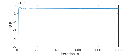
(a) TV-deblurring
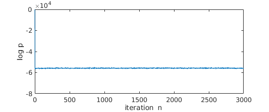
(b) TGV-denoising
Conversely, if plots show that the chain is divergent or very unstable, then there might be a problem with the sampler. A common cause for divergence is setting a discretisation step-size that is too large. We would advise not to proceed with the estimation of until the sampler shows a stable behaviour similar to the ones shown on Figure 25.
B.2 Monitoring convergence in Algorithm 1, Algorithm 2 and Algorithm 3
Lack of convergence due to bound saturation
If one observes that the iterate saturates the limits of the projection interval , one should first verify that the Markov kernels are working properly (see recommendations in B.1). If they are, then the problem might be that the solution lies outside . If is multivariate and only some components are saturating the bounds, then check the scale and projection bounds for those specific components.
Verifying proper convergence
As the algorithm converges, the iterates get closer to a maximiser of and the gradient estimates vanish in expectation. Hence, the residual should become small (on average) as increases, i.e., will become close to in Algorithm 1, or close to in Algorithm 3101010For Algorithm 2 use a component-wise comparison between and for every . It is therefore useful to plot the traces of together with or as appropriate, to check that the algorithm is converging. The trace can be plotted for a fixed value of as this is enough to monitor the convergence. This is illustrated for Algorithm 3 in Figure 26 below, where we observe how these terms become closer as the number of iterations increases.
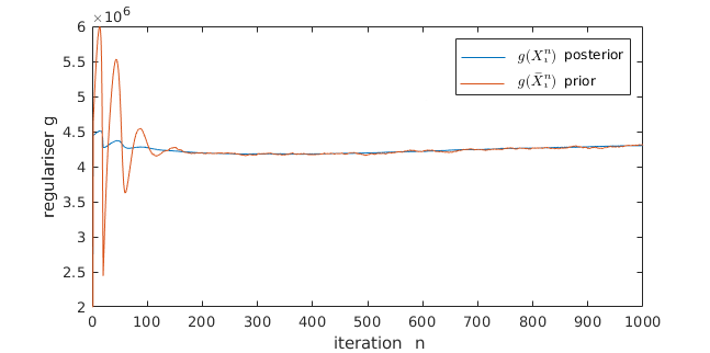
If does not vanish as increases this could indicate a problem with the choice of or that the two MCMC kernels have very different speed (See Section B.3).
B.3 Working with two MCMC chains in Algorithm 3
Using two MCMC kernels simultaneously can be problematic if their convergence speed, or effective sample size per iteration, is very dissimilar as this will deteriorate the convergence properties of the SAPG algorithm.
This kind of imbalance can be detected by plotting the sample autocorrelation for each chain using as a summary statistic. If the autocorrelation plots decay at significantly different rates, it is necessary to reduce the correlation within the slower chain by either introducing some thinning (which essentially amounts to concatenating several iterations of the kernel to improve its convergence speed) or by increasing the step-size (see Section B.5).
B.4 Working with multivariate
When is multivariate each component of the solution might have a different order of magnitude. In this case, we recommend using different step-size scales for each component of . For example, we can compute , where is a diagonal matrix, and each element of the diagonal scales one component of . It is also helpful to remember that one can run the algorithm with some components of fixed. This allows isolating components and verifying convergence for subsets of .
B.5 Convergence speed
The bottleneck in convergence speed is the correlation between the samples generated by the MCMC kernels. To increase the convergence speed, one has two main alternatives: a) to reduce the correlation between samples, or b) to reduce the computational cost of each iteration in order to afford more iterations.
Reducing sample correlation
To reduce the correlation between samples, the step-size must be as large as possible. If running the algorithm with two chains, and the kernel sampling from the prior distribution is the limiting factor, one can consider increasing the smoothing parameter of this particular kernel, in order to be able to increase the value of the discretisation step-size . In more general cases where the limiting factor for is there are a few strategies that might help overcome this difficulty. The first strategy is to use preconditioning (see the hyperspectral unmixing experiment in Section 4.3) to reduce gradient anisotropy and improve the condition number of the problem.
Speeding up each iteration
The most computationally heavy step in a MYULA iteration is usually the evaluation of the proximal operator. If the proximal operator is being approximated by an iterative solver, it is worth trying to improve efficiency by either using better solver, by warm starting iterations, or by using a weaker convergence criterion.
B.6 Estimation Bias
If the algorithm converges but towards a poor value of it might be due to the bias in the MCMC kernels. As mentioned previously, there are many levels of approximation and the bias is mostly affected by the discretisation step and the smoothing parameter . However, based on what we have observed in practice, the limiting factor tends to be . If there is a bias issue, we recommend trying to reduce to obtain a better approximation of the target distribution, at the expense of some deterioration in convergence speed. When convergence is slowed down, special attention has to be paid in the case of the double MCMC chain algorithm. If the effective sample size of the two chains becomes too dissimilar, the algorithm might have difficulty converging. In this case, it is possible to do some thinning in the slower chain, as suggested in Section B.3.
Appendix C Fair comparison of different methodologies
Comparing different techniques for selecting the value of the regularisation parameter is highly non-trivial. Methods such as SUGAR are solver dependent and try to find the best value of for a given solver, with a given setup (number of iterations, parameters, etc.). Other algorithms such as the hierarchical one proposed in [53], depend on the solver but do not seek to optimise for that particular solver. The algorithm we propose does not depend directly on the solver.
When running statistics on our experiments we noticed an interesting phenomenon. For the deblurring experiments, we use the solver SALSA [1], which is an efficient implementation of the alternating direction method of multipliers (ADMM). When running the hierarchical Bayesian algorithm, we implement it with SALSA and set up the tolerance to and 150 iterations which seemed sufficient to render very good results. However, when we build the MSE() curves for Figure 14 (by sampling many points and interpolating), we use SALSA with tolerance and 1000 iterations as there were some values of for which SALSA did not converge well with tolerance . See in Figure 27 that the position of the minimum MSE changes for the two different SALSA configurations. When computing the average results for 10 images, the parameters obtained with the hierarchical method fell closer to the minimum of the red curve, and the ones obtained with the proposed empirical method fell closer to the minimum of the blue curve. Running the hierarchical method with tolerance produced similar results but significantly increased the computing times.
The criterion we opt for was to use SALSA with the strictest tolerance and highest number of iterations, because this configuration gives the overall best estimations.
C.1 Comparing with solver-dependent methods
As mentioned previously, algorithms like SUGAR try to find the best value of for a given solver, with a given number of iterations, and specific parameters. This means that unless SUGAR is implemented with the exact same solver used to construct the curves as the ones in Figure 27, the values of computed with SUGAR might yield poor results according to the curve but good results with the specific solver used in SUGAR. For this reason, to achieve a fairer comparison, we compute an equivalent in the following way. The SUGAR algorithm returns an estimated and a corresponding obtained with that . Given an curve, we define the equivalent as , which we plot in Figure 7.
