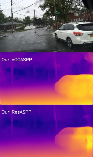
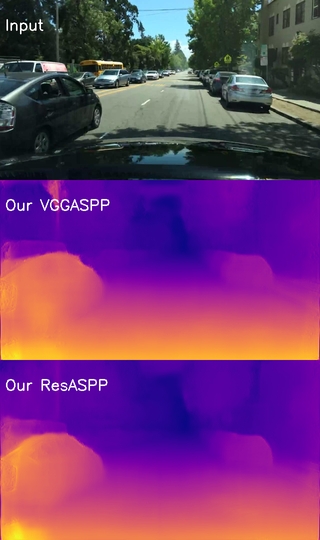
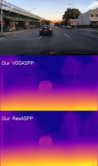
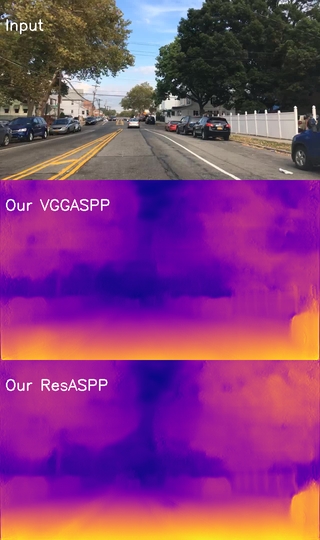
Edge-Guided Occlusion Fading Reduction for a Light-Weighted Self-Supervised Monocular Depth Estimation

Abstract

Self-supervised monocular depth estimation methods generally suffer the occlusion fading issue due to the lack of supervision by the per pixel ground truth. Although a post-processing method was proposed by Godard et. al. [1] to reduce the occlusion fading, the compensated results have a severe halo effect. In this paper, we propose a novel Edge-Guided post-processing to reduce the occlusion fading issue for self-supervised monocular depth estimation. We further introduce Atrous Spatial Pyramid Pooling (ASPP) into the network to reduce the computational costs and improve the inference performance. The proposed ASPP-based network is lighter, faster, and better than current commonly used depth estimation networks. This light-weight network only needs 8.1 million parameters and can achieve up to 40 frames per second for $256\times 512$ input in the inference stage using a single nVIDIA GTX1080 GPU. The proposed network also outperforms the current state-of-the-art on the KITTI benchmarks. The ASPP-based network and Edge-Guided post-processing produce better results either quantitatively and qualitatively than the competitors.

Keywords Self-supervised  $\cdot$ monocular depth  $\cdot$ occlusion fading  $\cdot$ edge-guided  $\cdot$ atrous spatial pyramid pooling

1 Introduction

Depth estimation is one of the fundamental problems with a long history in computer vision. It also serves as the cornerstone for many machine perception applications, such as 3D reconstruction, auto-driving system, industrial machine vision, robotics interaction, etc. However, most research is performed based on the availability of multiple observations in target scenes. The constraint of the multiple observations can be overcome by the supervised method because of the emerging deep learning technology [2, 3, 4]. These methods aim to directly predict the pixel depth from a single image by learning the given ground truth depth data of a large amount of dataset. Despite the promising results of the monocular depth prediction, these methods suffer from the limitation of the quality and availability of the collected ground truth pixel depth. Hence, the self-supervised approaches learning the depth information from a single image has received increasing attention in recent research.

Figure 1: Comparison between the conventional post-processing (PP) [1] and the proposed Edge-Guided post-processing (EG-PP) on KITTI dataset. Our method can reserve the sharp edge of the detected object depth and avoid the halo effect.

In the task of monocular depth estimation, the input source is a monocular image (e.g., a left image) and the stereo pairs are available during training. Then the corresponding another view (e.g., the right image), can be reconstructed by the estimated right depth and the input left image (left) using a warping function [5]. Hence, the reconstructed right view is supervised by an actual right image. The estimated depth can also be calibrated in the regression for the reconstructed right view. One of the major challenges of the self-supervision method is to reduce false detection using a compact network. It’s been shown in [1] that the deeper network (e.g. Resnet50) can yield better estimated depth compared to a compact network (e.g. VGG19). However, very deep networks are inefficient for real-time usage. A high performance light-weight network design for a depth estimation network is needed. Another challenge is the stereo dis-occlusion effect. Disparity ramps happen in the stereo dis-occlusion area of the estimated disparity and largely downgrade the estimation quality quantitatively and qualitatively. Although a post-processing method is proposed to compensate the occlusion shading using a flip prediction alignment method [1], the compensated output suffers severe halo effect as shown in Fig. 1(PP). A solution of solving this issue requires high quality estimation results.

The main contributions of this paper are as follows: (1) We propose a Light-weight DispNet that is smaller, faster, and better than the conventional DispNet. We also point out that the last two dense feature layers of the encoder in DispNet are less efficient in extracting long-range features. (2) A novel Edge-Guided post-processing method is presented in this paper. The occlusion fading is largely reduced with a minimized halo effect after applying our method. This Edge-Guided post-processing is universal and can be applied to any other self-supervised method. (3) We evaluate our approach compared to the state-of-the-art on the challenging KITTI dataset. We test both the intrinsic network and integrated performance separately to demonstrate that our method has fundamentally improved the network performance. In the integration test, we showcase that our results can compete with the method that uses the semantic consistency supervision.

2 Related Works

A depth map is a form of an absolute depth or disparity value. The depth is inversely proportional to the disparity. The former and latter values can be converted to each other based on the parameters of the rectified multi-cameras. We use monocular depth estimation because they use a single monocular image as the input to the system rather than using multi-view images to calculate the disparity of the scene [6]. In [4], CNNs and continuous CRFs are used as a patch-wise depth predictor to estimate the depth information in a supervised manner, which required a large amount of high-quality ground truth images. A combination of coarse and fine cues was proposed to improve the performance of the depth estimation but still was supervised [7]. On the other hand, self-supervised approaches only need supervision from either stereo image pairs [8, 1, 9] or monocular video frames [10, 11, 12, 13, 14, 15]. In this approach, the disparity is used as an intermediate product which can be converted to reconstruct the images with the inverse warping transform [5]. To improve the performance of the self-supervised algorithm, various objective functions are proposed, such as left-right consistency [1], correlational consistency [16], and adaptive global and local error [9].

Self-supervised approaches have limited predictive abilities on finer details in an image compared to their supervised counterparts. There were different methods devised to mitigate this limitation. A semi-supervised approach is a combination of self-supervised and supervised methods [17, 18] . These approaches predict the dense pixel depth on pixels with ground truth from the supervised information and the pixels without ground truth in the self-supervised approach. These methods were particularly useful when the ground truth was sparse, and they yield promising results. Rather than using ground truth information, a joint prediction approach can use the semantic segmentation to assist in depth estimation [19]. In semi-supervised approaches, the implicit methods were used to predict the depth and semantic segments jointly to leverage the common feature representations between two tasks; however, each task used independent objective functions [20, 21, 22, 23]. More recent work introduced the depth-semantic gradient consistency explicitly to refine the fine details of the estimated depth map [24, 25, 26, 19].

One limitation of self-supervision method was the stereo dis-occlusion effect. The self-supervision method relied on stereo image pairs to calibrate the estimation without the ground truth. This method inherits the stereo dis-occlusion effect from the objective function that uses stereo image pairs. The early researches in the occlusion detection used Bayesian formulation [27], AdaBoost [28], and Random Forest based framework [29] to detect the motion occlusion regions of motion images. These priors handcrafted the features to proceed the machine learning algorithms. Recently, a learning-based method has considered structural left-right symmetry [30] to detect occlusions, while a[31] proposed to estimate occlusions, motion, and depth boundary using a single network. These prior had shown plausible results but need a complicated model to only detect the occlusion. Recently, [1] proposed to use a simple post processing module of flip prediction alignment method to recover the information of the occlusion area for the self-supervision approaches. Unfortunately, halo effects occur after applying this post processing module to the estimation. None of the current methods can fit the needs of reducing the occlusion fading for a self-supervised depth estimation task.

In this paper, we improve the depth network efficiency and performance quantitatively and qualitatively. However, there are only a few works that focus on optimizing the network structure for self-supervision in real-time. A Light-Weight RefineNet was proposed for joint semantic segmentation and depth estimation task [32]. This methods is designed for the supervision method. We have tested it and found out that its performance is limited when applying to the self-supervision method. When we studied the multi-task network, we realized that the depth estimation and semantic segmentation can share the same feature representation in the network. Based on this finding, we argue that the semantic segmentation network structure can be used in the depth estimation network. In this paper, we introduce Atrous Spatial Pyramid Pooling (ASPP) module into our depth network from Deeplab semantic segmentation network [33]. We successfully designed a Light-weight DispNet that has only $20\%$ size of the conventional depth network but is about $35\%$ faster in prediction. To address the occluding fading issue, we proposed an Edge-Guided post-processing method using Tensorflow right after the depth network to eliminate the occluding fading and halo effects in inference stage. The proposed method effectively improve both the quantitative and qualitative results and is suitable for all the self-supervision-based methods.

3 Methodology

Our model is inspired by the works of [33] and [1]. We first introduce the ASPP module [33] into our network design, and then the objective function is directly adopted from [1]. The proposed Edge-Guided post-processing is explained in the last section.

3.1 Light-Weight Disparity Network

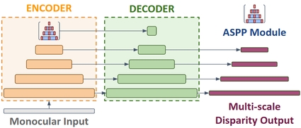
Many recent works designed their network by referring to DispNet [34], which is an autoencoder-based architecture. The multi-scale features are exploited from the encoder, and the spatial resolution is recovered from the decoder. The recovered multi-scale spatial resolutions are the estimated disparities.

Since it has been shown that the depth estimation and semantic segmentation prediction have common feature representations and they can share the base-network to perform multi-task prediction [35], we use the network design concept of the semantic segmentation task. It indicates that an extra module is commonly cascaded on top of the original network for detecting long-range information [33, 36]. We follow this design rule to modify the DispNet to do the depth estimation. We choose the ASPP module [33] as our long-range detection module and insert it between the encoder and decoder.

To further optimize our network, we analyzed the feature layers of the encoder, and we found that the last few dense feature layers have a minor contribution to the estimation, especially after introducing the ASPP module. Based on this observation, we simplify the DispNet by using ASPP module to replace the last two dense layers of the encoder. This design successfully reduces the network size of the network and produce a better performance. We name this structure a Light-Weight DispNet. The proposed network structure is shown in Fig. 2. We here use [1] as a baseline example. If DispNet uses VGG19 as the backbone, the network parameters are about 31.6 million, and the inference time is about 32 msec. The corresponding Light-Weight DispNet only need 8.1 million ($74\%$ less) with inference time 25.2 msec ($22\%$ less). Nevertheless, the proposed Light-Weight DispNet inherits the trait of DispNet that the backbone of the encoder can be modified. In this paper, we choose VGG8 and Resnet24 as our backbones. We demonstrate that the ASPP can effectively improve the estimation performance in our evaluation. Please refer to Appendix for the detailed network design.

Figure 2: Light-Weight DispNet Structure.

3.2 Objective Function

We decide to adopt the objective function from [1] directly with several reasons. The most important consideration is that the aim of the left-right consistency function from [1] has demonstrated promising results among the recent works. The successors only have minor modifications. Besides, we would like to showcase that the proposed Light-Weight DispNet is substantially better than the conventional DispNet using the same objective function.

The objective function is a weighted sum of three terms: appearance $(C_{ap})$, disparity smoothness $(C_{ds})$, and left-right consistency $(C_{cor})$. The self-supervise total loss is defined as following:

$$C_{s}=\alpha_{ap}\times C_{ap}+\alpha_{ds}\times C_{ds}+\alpha_{lr}\times C_{cor}$$ (1)

The weights $(\alpha_{ap},\alpha_{ds},\alpha_{lr})$ are determined before optimization and set as $(1.0,0.5,1.0)$. The definition of each term can be found in [1].

Figure 3: Edge-Guided Post Processing

3.3 Edge-Guided Post-Processing

The stereo dis-occlusion effect is one of the limitations in the self-supervision method of monocular depth estimation. Stereo dis-occlusion creates disparity ramps (occlusion fading) on both the left side of the image and the occluders. [1] proposed a post-processing method to reduce this effect. This post-processing estimates the disparity map $d_{l}$ and the flipped disparity map $d^{\prime}_{l}$, which are from input image $I$ and its horizontally flipped image $I^{\prime}$. Then the flipped disparity map $d^{\prime}_{l}$ is flipped back as a $d^{\prime\prime}_{l}$ that aligns with $d_{l}$ but where the occlusion fading is on the right of occluders as well as on the right side of the image. The final result is an average of $d_{l}$ and $d^{\prime\prime}_{l}$ but assigning the first $5\%$ on the left of the image using $d_{l}$ and the last $5\%$ on the right to the disparities from $d_{l}$. The $5\%$ of left and right original disparities is the reserved boundary range to avoid the boundary fading during the disparity synthesis in the post processing.

This post-processing uses a mirror trick to generate a well-aligned projected disparity $d^{\prime\prime}_{l}$ that has right-side occlusion fading. The average of $d_{l}$ and $d^{\prime\prime}_{l}$ can reduce the left-side occlusion fading because $d^{\prime\prime}_{l}$ has correct left-side estimation results. However, the right-side occlusion fading is also being involved. This average process in the post-processing causes the halo effect in the final results, as shown in PP of Fig 1. Instead of average, we propose an Edge-Guided weighted sum to suppress the occlusion fading of both $d_{l}$ and $d^{\prime\prime}_{l}$ in the combination to reduce the halo effect, as shown in EG-PP of Fig 1.

The proposed Edge-Guided post-processing is depicted in Fig. 3. We follow the design concept of [1] to compute $d_{l}$ and $d^{\prime\prime}_{l}$, but we add edge-aware weights ($w$, $w^{\prime\prime}$) in the final combination. Here we take $w$ as an example to illustrate the algorithm. A right-edge detector is designed to extract the regional-edge confidence $E$. Instead of using Sobel detector, a wide-range horizontal gradient filter ($f_{gx}$) is used:

$$f_{gx}=\begin{bmatrix}1&...&0&-1&...\\ 1&...&0&-1&...\\ 1&...&0&-1&...\end{bmatrix}_{3\times(2N)}/(3\times(2N))$$ (2)

where $N$ is the detection radius, whose default value is set to 10. After the convolution process $(\otimes)$ of $d_{l}$ and $f_{gx}$, we add an offset ($b$) and a gain ($a$) on the convolution result. Then a sigmoid function is applied:

$$E_{l}=\text{sigmoid}((d_{l}\otimes{f_{gx}}-b)*a)$$ (3)

where $E_{l}$ is the right regional-edge confidence. The offset $b$ and gain $a$ are set as 0.5 and 32 to maximize the $E_{l}$ in the range [0, 1]. In this equation, the right edge region has the confidence close to 1, while the left occlusion fading area has the confidence close to 0. The confidence of the flat area keeps around 0.5. The $E^{\prime\prime}_{l}$ is obtained in the same way but using the horizontal flipped $f_{gx}$ as the left-edge detector. The last step is to normalize $E_{l}$ and $E^{\prime\prime}_{l}$ to obtain $w$ and $w^{\prime\prime}$. Then the final output $d^{\star}_{l}$ is a weighted sum of $d_{l}$ and $d^{\prime\prime}_{l}$:

$$w=E_{l}/(E_{l}+E^{\prime\prime}_{l})$$ (4)

$$w^{\prime\prime}=E^{\prime\prime}_{l}/(E_{l}+E^{\prime\prime}_{l})$$

$$d^{\star}_{l}=wd_{l}+w^{\prime\prime}d^{\prime\prime}_{l}$$ (5)

The normalization process is needed to prevent overlap detection between $E_{l}$ and $E^{\prime\prime}_{l}$. It ensures that the sum of $w$ and $w^{\prime\prime}$ is 1 for each pixel and the final output $d^{\star}_{l}$ has no overhead compared to $d_{l}$ and $d^{\prime\prime}_{l}$. There are no learning parameters and the computation cost is very low. We also follow the boundary reserving design here with the $2\%$ reserved boundary range. The details are described in Appendix.

4 Experiments

We compare the performance of our approach to recent self-supervised monocular depth estimation methods. We selected Godard et al. [1]’s work as our baseline and used the same benchmark configurations [1]. We evaluate our approach in multiple aspects of KITTI [37] dataset quantitatively and qualitatively. The ablation study is first conducted to prove the effectiveness of our approach using KITTI split. We then have a benchmark with the current start-of-the-art on Eigen split. We split the benchmark into two parts: network and integration test. In the network test, we showcase that the proposed network structure is better than the competitors without any post-processing. The integration test is to demonstrate the power of the proposed Edge-Guided post-processing method. We involve the semantic consistency of semi-supervision learning [19]. Please refer to our code to see the detailed implementation.

4.1 Datasets

We evaluate the performance of the proposed method on the KITTI benchmark [37]. We use two different test splits, KITTI and Eigen Split [3], of KITTI dataset to do the ablation analysis of the variants of our method and the benchmark compared with the existing works. We follow the approach of [1] to use 29,000 image pairs as the training set. The typical image size of the KITTI dataset is $375\times 1242$ pixels, and the stereo image pairs are well-calibrated in the calibrated camera configuration. The depth labels were collected from a Velodyne laser sensor.

Furthermore, it has been shown by [1] that pre-training with Cityscapes dataset [38] can improve the performance on KITTI benchmark. We also include this strategy in the benchmark. Cityscapes dataset contains 22,973 higher resolution and image quality training stereo pairs. We use the same crop as [1] to avoid the reflective car hoods from the input. In the combinational training on Cityscapes and KITTI dataset (C+K), we pre-train our models with an eight batches and 50 epochs initial training on Cityscapes dataset, and then another eight batches and 100 epochs training on KITTI dataset.

4.2 Metrics

We use the evaluation metrics from [37] for depth estimation, which measure the error in meters from the ground truth and the percentage of depth that is within a threshold from the correct value. The error measurements represent the average error.

4.3 Implementations

Configuration

Our methods were implemented in Tensorflow 1.15 [39] using Python 3.7 under the Ubuntu environment with a single NVIDIA GTX 1080 GPU. All input images are resized to $256\times 512$ from the original size of the training image. All our models are trained by eight batches and 100 epochs on the KITTI training dataset. The predictions happen in around 25ms (around 40 frames per second (FPS)) of the proposed VGGASPP model and 31ms (around 33 FPS) of the proposed ResASPP model.

Parameter Settings

We follow the prior work [1] to set up the training optimizer and parameters. We train our models from scratch and use the Adam optimizer. The training flow involves a batch size 8 and 100 epochs. The model converges after 80 epochs, and the improvement after 100 epochs was minor.

Network Backbone

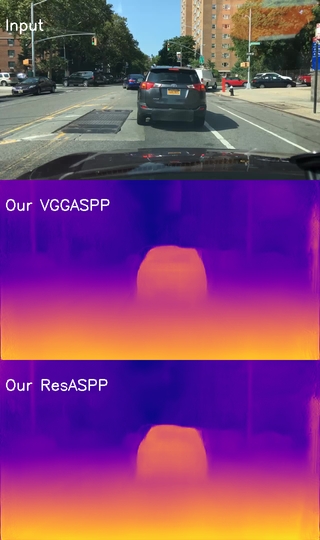
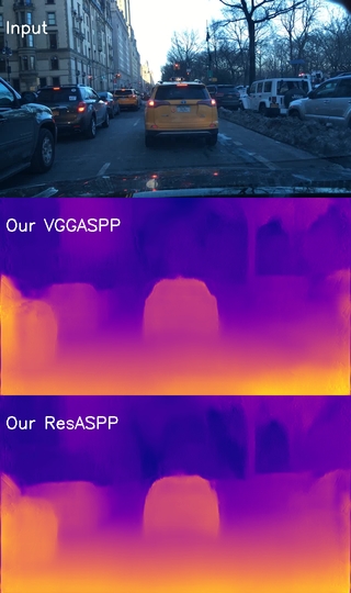
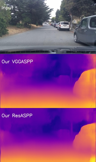
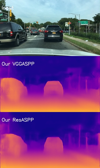
In the evaluation, we show the experimental results in two models, VGGASPP (VGG8 Backbone) and ResASPP (Resnet24 Backbone), of our Light-weight DispNet. The computation costs of each backbone are also summarized in the Ablation section. We show that both our models have better performance than competitors in the benchmark studies.

4.4 Results

4.4.1 Ablation Study

In the ablation study, we analyze the quantitative performance improvement and the computational costs of our various designs using KITTI split on the KITTI dataset. For the quantitative performance improvement, we use two models, VGG and Resnet50, of our prior work [1] without post-processing as the baseline. The results are shown in Table 1. We can see that our VGGASPP without conventional post-processing outperforms the VGG model of the baseline and is very close to the Resnet50 one. On the other hand, our ResASPP without conventional post-processing has better performance than both VGG and Resnet50 models on the baseline. Furthermore, compared to the conventional post-processing, the proposed Edge-Guided post-processing has a significant performance boost on both our two models, especially on terms of RMSE(log) and $\delta<1.25$, which are the most challenging parts. We also add the C+K training set up in the last section. We found that our VGGASPP can even outperform ResASPP using the Edge-Guided post-processing.

Approach	Train	PP	ARD	SRD	RMSE	RMSE(log)	D1-all		$\delta<1.25$	$\delta<1.25^{2}$	$\delta<1.25^{3}$
			Lower is better.						Higher is better.
Godard et al. [1] VGG	K	N	0.1240	1.3880	6.125	0.217	30.272		0.841	0.936	0.975
Godard et al. [1] Resnet50	K	N	0.1127	1.1331	5.749	0.203	29.553		0.851	0.947	0.980
Our VGGASPP	K	N	0.1134	1.1636	5.734	0.201	27.379		0.853	0.945	0.979
Our VGGASPP	K	Y	0.1079	1.0259	5.464	0.192	26.395		0.857	0.949	0.982
Our VGGASPP	K	Y+	0.1077	1.0238	5.387	0.189	26.152		0.860	0.951	0.983
Our ResASPP	K	N	0.1107	1.0633	5.612	0.199	27.531		0.854	0.946	0.980
Our ResASPP	K	Y	0.1075	0.9878	5.474	0.193	27.050		0.855	0.949	0.981
Our ResASPP	K	Y+	0.1071	0.9936	5.394	0.189	26.673		0.858	0.952	0.983
Our VGGASPP	C+K	Y+	0.0984	0.9196	5.035	0.175	22.942		0.883	0.961	0.986
Our ResASPP	C+K	Y+	0.1000	0.9697	5.070	0.175	23.231		0.879	0.961	0.987

Table 1: Quantitative results for different variants of our approach on the KITTI Stereo 2015 test dataset. The PP means using post-processing. N means no PP, Y means conventional PP, and Y+ represents the proposed Edge-Guided PP. The best result in each subsection is shown in bold. The training scenario is based on the KITTI training set (K), while the last section shows the results which are pre-trained by Cityscapes training sets (C+K). We use our prior [1] as our baseline is shown in the first section.

In Table 2, we can see the computation costs of both our methods with the baseline. Our VGGASPP has only $25.6\%$ of parameters but is $23.2\%$ faster in the prediction compared to VGG model of the baseline. Our ResASPP has only $13.8\%$ of parameters but performs $48\%$ more quickly in the prediction compared to the Resnet50 model of the baseline. Only $3.8\%$ and $3\%$ loss in computation time occur in prediction on VGGASPP and ResASPP models when we apply the Edge-Guided post-processing to our methods. There is no need for extra parameters.

Approach	Parameters	Predict(ms/FPS)
Godard et al. [1] VGG	31600072	31/32.2
Godard et al. [1] Resnet50	58452008	44/22.7
Our VGGASPP	8134344	25.2/39.7
Our ResASPP	11825448	29.7/33.6
Our VGGASPP+EGPP	8134344	26.2/38.2
Our ResASPP+EGPP	11825448	30.6/32.6

Table 2: Computational costs of different variants of our approach on the KITTI training dataset within 8 batches and 100 epochs. The units of training of prediction are msec(ms) and frame per second(FPS). Smaller parameters and ms values represent lower cost.

4.4.2 State-of-the-art comparison

Approach	Train	Test	PP	ARD	SRD	RMSE	RMSE(log)		$\delta<1.25$	$\delta<1.25^{2}$	$\delta<1.25^{3}$
				Lower is better.					Higher is better.
Zhou et al. [11]	K	E - 80m	N	0.2080	1.7680	6.8560	0.283		0.678	0.885	0.957
Mahjourian et al. [13]	K	E - 80m	N	0.1630	1.2400	6.2200	0.25		0.762	0.916	0.968
Garg et al. [8]	K	E - 80m	N	0.1520	1.2260	5.849	0.246		0.784	0.921	0.967
Godard et al. [1]	K	E - 80m	N	0.1480	1.3440	5.927	0.247		0.803	0.922	0.964
Alex and Stefano [9]	K	E - 80m	N	0.1330	1.1260	5.515	0.231		0.826	0.934	0.969
Ours VGGASPP	K	E - 80m	N	0.1146	1.0248	5.198	0.217		0.851	0.936	0.970
Ours ResASPP	K	E - 80m	N	0.1124	1.0002	5.129	0.215		0.855	0.938	0.971
Zhou et al. [11]	C+K	E - 80m	N	0.198	1.836	6.565	0.275		0.718	0.901	0.96
Mahjourian et al. [13]	C+K	E - 80m	N	0.159	1.231	5.912	0.243		0.784	0.923	0.97
Godard et al. [1]	C+K	E - 80m	N	0.1240	1.0760	5.311	0.219		0.847	0.942	0.973
Alex and Stefano [9]	C+K	E - 80m	N	0.1180	0.9960	5.134	0.215		0.849	0.945	0.975
Ours VGGASPP	C+K	E - 50m	N	0.1095	0.9405	5.001	0.208		0.864	0.944	0.974
Ours ResASPP	C+K	E - 50m	N	0.1077	0.9303	4.954	0.208		0.865	0.944	0.974
Garg et al. [1]	K	E - 50m	N	0.1690	1.0800	5.1040	0.273		0.740	0.904	0.962
Zhou et al. [11]	K	E - 50m	N	0.2010	1.3910	5.1810	0.264		0.696	0.900	0.966
Godard et al. [1]	K	E - 50m	N	0.1400	0.976	4.471	0.232		0.818	0.931	0.969
Alex and Stefano [9]	K	E - 50m	N	0.1260	0.832	4.172	0.217		0.840	0.941	0.973
Ours VGGASPP	K	E - 80m	N	0.1077	0.7273	3.885	0.204		0.865	0.944	0.974
Ours ResASPP	K	E - 80m	N	0.1058	0.7211	3.846	0.202		0.868	0.945	0.974

Table 3: Quantitative results of network test compared with the state-of-the-art on KITTI Eigen (E) split with KITTI (K) training set. For a fair comparison, we compare the reference methods without the post-processing (PP), and all the results use the crop defined by [8]. We also examine the effects of the full distance (0-80m) and the near distance (1-50m). The results which are pre-trained with Cityscapes (C) are evaluated as well.

Figure 4: Benchmark of qualitative results on KITTI dataset Eigen Split. All the results have no post-processing for a fair comparison. There are are many missing and false detection of trunks, poles, trucks, or cars in the reference methods. By contrast, our methods can accurately capture more fine objects and maintain their shapes better.

Network Test

The network test considers the performance of the network without help from any post-processing methods in Table 3. We involve several self-supervised priors, and the test is based on Eigen-slipt of KITTI dataset. The test is essentially in two types of examination, namely the results of the full distance (0-80m) and near distance (1-50m). We use the same crop defined by [8] for a fair comparison. The training set is the KITTI dataset only, and we also add other C+K full distance results in the second section of the table. In the case of the KITTI dataset, our methods largely outperform all the competitors in all metrics. In terms of $\delta<1.25^{2}$ and $\delta<1.25^{3}$, we have only minor improvement since the results of these two metrics are nearly saturated. In the case of C+K, our results are significantly better than all the competitors except for the last two accuracy terms. We also found that our ResASPP model has a better performance than VGGASPP in all cases.

Approach	Train	Test	PP	ARD	SRD	RMSE	RMSE(log)		$\delta<1.25$	$\delta<1.25^{2}$	$\delta<1.25^{3}$
				Lower is better.					Higher is better.
Godard et al. [1]	K	E - 80m	Y	0.1480	1.3440	5.927	0.247		0.803	0.922	0.964
Po-Yi et al. [40] - w/ seg	K	E -80m	Y	0.1180	0.9050	5.096	0.211		0.839	0.945	0.977
Ours VGGASPP	K	E - 80m	Y+	0.1070	0.9055	4.873	0.202		0.862	0.945	0.975
Ours ResASPP	K	E - 80m	Y+	0.1073	0.8849	4.866	0.203		0.862	0.945	0.975
Godard et al. [1]	C+K	E - 80m	Y	0.1140	0.8980	4.935	0.206		0.861	0.949	0.976
Ours VGGASPP	C+K	E - 80m	Y+	0.1008	0.6462	3.653	0.190		0.875	0.952	0.979
Ours ResASPP	C+K	E - 80m	Y+	0.1012	0.6425	3.645	0.190		0.875	0.952	0.979
Godard et al. [1]	K	E - 50m	Y	0.1400	0.9760	4.471	0.232		0.818	0.931	0.969
Po-Yi et al. [40] - w/ seg	K	E -50m	Y	0.1120	0.6730	3.871	0.198		0.852	0.951	0.980
Ours VGGASPP	K	E - 50m	Y+	0.1014	0.7942	4.627	0.192		0.876	0.953	0.979
Ours ResASPP	K	E - 50m	Y+	0.1008	0.8054	4.643	0.193		0.875	0.952	0.979
Godard et al. [1]	C+K	E - 50m	Y	0.1080	0.6570	3.729	0.194		0.873	0.954	0.979
Ours VGGASPP	C+K	E - 50m	Y+	0.0959	0.5853	3.486	0.181		0.887	0.958	0.981
Ours ResASPP	C+K	E - 50m	Y+	0.0950	0.5847	3.474	0.181		0.887	0.958	0.981
Godard et al. [1]	C+K	E - 80m(u)	Y	0.1300	1.1970	5.222	0.226		0.843	0.940	0.971
Ours VGGASPP	C+K	E - 80m(u)	Y+	0.1141	1.0460	4.884	0.210		0.861	0.946	0.975
Ours ResASPP	C+K	E - 80m(u)	Y+	0.1132	1.0419	4.895	0.210		0.861	0.946	0.975

Table 4: This table shows the intgration benchmark specifically compared with compared with Godard et al. [1] and Po-Yi et al. [40] with post-processing (PP). All the results still use the crop defined by Garg et al. [8] except for the last section, in which we evaluate the uncropped(u) results. In the PP column, Y means conventional PP, while Y+ means the proposed Edge-Guided PP. Overall, our results are better than the reference method in any scenario. The second reference [40] uses semantic segmentation as a reference to enhance the performance. We show that our method outperforms [40] even without the information of semantic segmentation. An interesting finding is that the VGGASPP and ResASPP have less difference when the proposed Edge-Guided PP is applied.

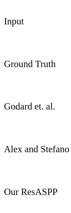
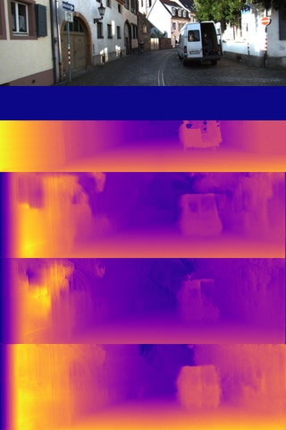
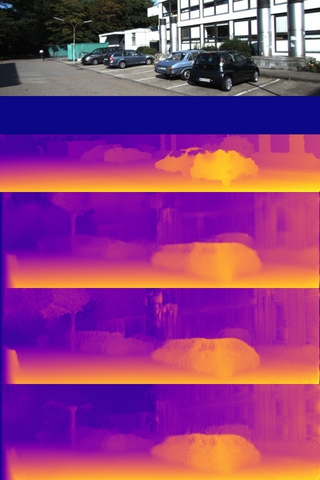
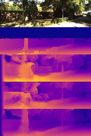
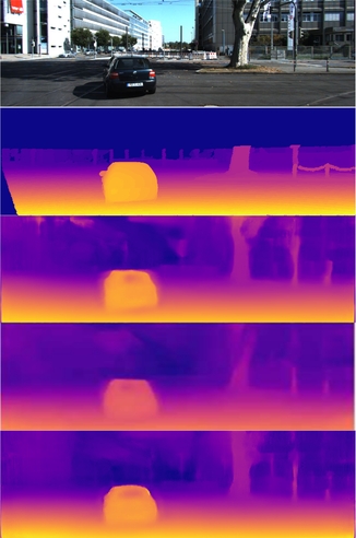
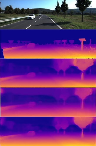
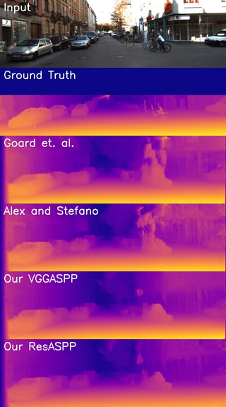
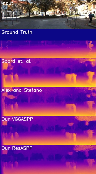
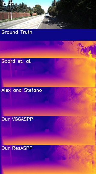
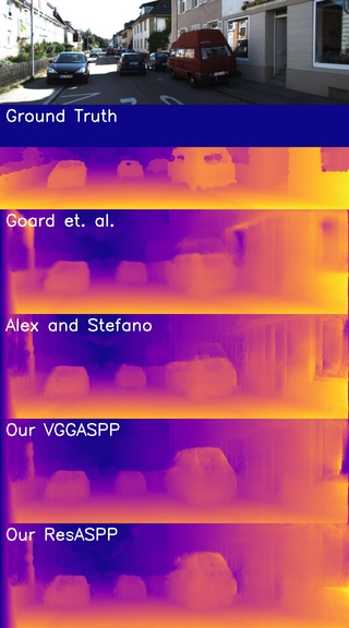
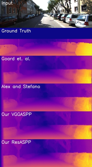
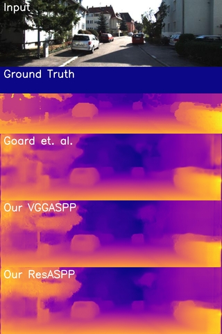
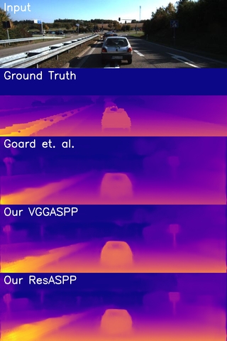
In the qualitative benchmark of network test, we choose the best two priors [1] and [9] as our references in Fig. 4. We demonstrate that our ResVGG has a better ability to capture either large size objects (e.g., trucks, cars, wall, etc.) and fine details (e.g., poles, trunks, signs, etc.). Our method has less false detection in the sky area. Our results are more clear and consistent with either the ground truth or the input image compared to the priors.

Figure 5: Benchmark of qualitative result on KITTI dataset KITTI Split. There are eight sets in two parts listed in the Figure. The images from top to down in each set are - source image, ground truth, Godard et al. [41], Po-yi et. al. [19], and our ResASPP. Our ResASPP has applied the proposed Edge-Guided post-processing. Our results can capture much more clear object shapes, such as signs, cars, and trunks than priors. The halo effects are also effectively reduced in our results.

Integration Test

In the integration test of our benchmark, we involve the post-processing in the comparison. To further showcase the power of the propose Edge-Guided post-processing, we add a special prior [19] that uses semantic consistency to capture better object shape in the estimated depth map. There are multiple scenarios in this test. From the training aspect of view, there are K only and C+K cases. In test cases, we still use Eigen-split with full and near distance under Garg [8] crop, but an uncropped full distance comparison is added at the end of the quantitative results of Table 4. Our results with conventional post-processing are still better than two competitors except for the last two accuracy terms in all cases. When we apply the Edge-Guided post-processing method, our results become significantly better, and only the last accuracy term is slightly behind.

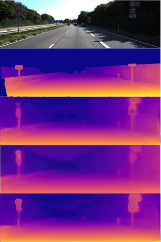
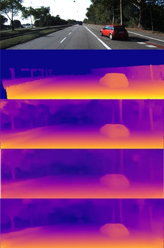
The improved performance of our method is not only quantitative, but also qualitative. The results are shown in Fig. 5. We use the same demo pictures as [19] to have a fair comparison. Our results have a much better ability to reproduce clear object shapes and edges in any size, especially the signs and trunks in the test images. The halo effects around objects (e.g., cars, signs, trunks,etc.) are largely reduced using the proposed Edge-Guided post-processing. In the visual evaluation, we provide much more accurate and visually appealing images to viewers.

In the qualitative benchmark, we include more results on KITTI dataset and extend our model on more datasets. Please refer to Appendix to check more results.

5 Discussion

In our benchmark, we have proved that the proposed Light-weight DispNet is better than related methods. The only difference is the introduced ASPP module to replace the last few dense feature extractor in the encoder. ASPP module has a smaller structure than the conventional dense feature extractors but can better detect long-range features.

The quantitative results have shown the improvement of the ASPP module, but we still have some limitations in the last two accuracy terms. These two terms indicate the coarse accuracy of the estimation. We can find that we mainly improve the object shape and clarity with ASPP, but no significant improvement in the rest flat area or very large object. The only improvement of the large area in the sky area that is not counted in the evaluation because there is no ground truth in this area. The current design of ASPP module has no significant impact on these parts. The possible solution is to improve the ASPP module further, e.g., enlarge the detection range, or add local-global information [42] to align the rest non-object area.

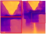
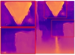
Although the halo effects have been largely removed using the Edge-Guided post-processing, there are still a few remaining halos. In this method, there are two assumptions: 1) the network can accurately capture the right-side edge of the object, and 2) the occlusion fading is inside the detection range. The first assumption indicates that the Edge-Guided method highly relies on the detection results of the network. If the network can only generate a blurred edge in the estimation, the performance of our method is limited. Furthermore, the detection range $N$ of our Edge-Guided method is also a trick. If we use a small $N$ in detection, the long occlusion fading can not be detected, and there will be a strong undershoot around the object contour in the final output. However, a large $N$ may involve unnecessary information to sabotage the detection results. Currently, we found that $N=10$ is the most balance setting, although there is still a bit remaining long-range fading as shown in Fig. 6. It may need a better edge detector to overcome this limitation.

(a) Conventional [1]

(b) Ours Edge-Guided

Figure 6: Post-processing performance comparison

6 Conclusion

We have presented a Light-weight DispNet and a novel Edge-Guided post-processing method to improve the performance for a self-supervised monocular depth estimator. Our primary contribution is that the proposed Light-weight DispNet demonstrates the inherent capability to capture long-range features to better estimate the depth map with a much smaller network structure compared to the current commonly used DispNet. We get up to a $48\%$ speed up in inference and $71.8\%$ fewer parameters of the network with a better performance both quantitatively and qualitatively. Another contribution of this work is that the Edge-Guided post-processing can resolve most occlusion fading effect of self-supervision methods. It can effectively reduce the halo effect that comes from the conventional post-processing to yield the object shape. The proposed Edge-Guided post-processing is an upgraded version of the conventional post-processing [1] and is suitable for all the self-supervised monocular depth estimators. The quantitative and qualitative results are both clear in the results. Our model only costs $4\%$ more in computation time, which is a very low price to improve the performance.

Appendix

Appendix A Network Architecture

In this section, we provide the network designs of our methods. The VGG and Resnet$\_$blocks are as the same as the conventional designs, but we remove the batch norm process of Resnet$\_$block. The ASPP module is directly adopted from the prior [33] in the implementation.

Layers	kernel	Ch I/O	Scale	input
VGG_block$\_$1	7	3/32	2	left
VGG_block$\_$2	5	32/64	4	VGG_block$\_$1
VGG_block$\_$3	3	64/128	8	VGG_block$\_$2
VGG_block$\_$4	3	128/256	16	VGG_block$\_$3
maxpool$\_$4	3	256/256	32	VGG_block$\_$4
ASPP	-	256/256	32	maxpool$\_$4

(a) Proposed VGGASPP encoder

Layers	kernel	Ch I/O	Scale	input
enc_block_1	conv$\_$7	7	2/64	2
enc_block_2	maxpool$\_$3	3	64/64	4
enc_block_3	Resnet_block	3	64/64	8
enc_block_4	Resnet_block	4	64/128	16
enc_block_5	maxpool$\_$3	3	128/128	32
enc_block_6	ASPP	128/256	32

(b) Proposed ResASPP encoder

VGG$\_$block
layers	kernel	stride	scale	input
conv1	k	2	2	block$\_$input
conv2	k	1	1	conv1
Resnet$\_$block
layers	kernel	stride	scale	input
conv1	1	1	1	block$\_$input
conv2	3	2	2	conv1
conv3	1	1	1	conv2
proj	-	-	-	block$\_$input+ conv3

(c) Backbone basic blocks

ASPP
layers	kernel	rate	Ch O	input
reduce$\_$mean	-	-	no change	block$\_$input
conv1	1	-	no change	reduce$\_$mean
upscale	-	-	no change	conv1
Astrous1	1	1	256	block$\_$input
Astrous6	3	6	256	block$\_$input
Astrous12	3	12	256	block$\_$input
Astrous18	3	18	256	block$\_$input
concat	-	-	-	upscale+ Astrous1+ Astrous6+ Astrous12+ Astrous18

(d) ASPP Module

Table 5: Proposed Network architecture, where k is the kernel size, Ch I/O is the number of input and output channels for each layer, Scale is the down-scaling factor for each layer relative to the input image, and input corresponds to the input of each layer where + is a concatenation and $\ast$ is a 2$\times$ upsampling of the layer.

Appendix B Edge-Guided Post-Processing

One of our major contribution is the Edge-Guided post-processing method that evolves from [1]. We further elaborate some detailed implementations that we haven’t mentioned in the main manuscript.

The conventional post-processing of [1] can be formulated as follows:

$$d_{l-syn}=d_{l}w_{l}+d^{\prime\prime}_{l}w^{\prime}_{l}+d_{lm}(1-w_{l}-w^{\prime}_{l})$$ (6)

$$d_{lm}=(d_{l}+d^{\prime\prime}_{l})/2$$

$$w_{l}(i,j)=\begin{cases}1&\text{if $j\leq{rng}$}\\ 0&\text{if $j>{rng}$}\\ 1-20\times(rng-j)&\text{else}\\ \end{cases}$$

where $d_{l-syn}$ is the synthesized left disparity, $d_{lm}$ is the modulated left disparity by $d_{l}$ and $d^{\prime\prime}_{l}$, $(i,j)$ are normalized pixel coordinates, $w_{l}$ is the per-pixel weight map, and $rng$ is the reserved boundary range that was set as 0.05 in [1]. This equation set shows that the left and right side has $5\%$ reserved range for $d_{l}$ and $d^{\prime\prime}_{l}$, while the center part uses $d_{lm}$ that is the the average of $d_{l}$ and $d^{\prime\prime}_{l}$. This is a boundary preserving design to avoid the boundary fading during the disparity synthesis in the post processing.

In our Edge-Guided post-processing, we introduced the edge-weighted left disparity as shown in Eq. (5) of the main script:

$$d^{\star}_{l}=wd_{l}+w^{\prime\prime}d_{l}$$ (7)

We also follow the boundary reserving design here and set the modulated left disparity $d_{lm}$ as $d^{\star}_{l}$. Furthermore, the reserved range $rng$ is only $2\%$ in our method. The final Edge-guided synthesized left disparity is as following:

$$d^{\star}_{l-syn}=d_{l}w_{l}+d^{\prime\prime}_{l}w^{\prime}_{l}+d^{\star}_{l}(1-w_{l}-w^{\prime}_{l})\\$$ (8)

We visualize the results of $d_{l}$, $d_{l-syn}$, $d^{\star}_{l}$, and $d^{\star}_{l-syn}$ to show the improvement of our method in Fig. 7. In the bounding boxes 1 and 2 show the occlusion fading reduction with the minimal halo effect of our method. In the bounding box 3, the boundary gradation of $d^{\star}_{l}$ can be improved by using the boundary preserving method. The $d^{\star}_{l}$ and $d^{\star}_{l-syn}$ in Fig. 7 have a few color difference of the color-mapping due to the value range variation between two results.

Figure 7: Comparison between the conventional post-processing (PP) [1] and the proposed Edge-Guided post-processing (EG-PP) on KITTI dataset. $d_{l}$ is the left disparity, $d_{l-syn}$ is the synthesized left disparity of [1], $d^{\star}_{l}$ is the proposed edge-weighted left disparity without the boundary preserving, and $d^{\star}_{l-syn}$ is the proposed edge-weighted left disparity with the boundary preserving. Our $d^{\star}_{l}$ and $d^{\star}_{l-syn}$ can reduce the occlusion fading well with minimal halo effects compared to $d_{l-syn}$ shown in the bounding boxes 1 and 2. The boundary preserving method works effectively to reduce the boundary gradation shown in the bounding boxes 3 of $d^{\star}_{l}$.

Appendix C Experiments

There are two updates in our experiments setup. The first update is the training setup. We originally used 8 batches and 100 epochs (8x100) on the KITTI training dataset, while in the C+K training case we train (8x50) on Cityscapes dataset and another 8x100 on KITTI dataset. However, we actually only used 8x50 on KITTI dataset of the C+K training case to get a optimal result and we would like to correct this wrong description.

The second update is the parameter optimization of the reserved boundary range ($rng$) in the Edge-Guiding post-processing. Originally, we applied the same $rng$ (0.05) as the prior [1] and we further optimized it to 0.02 due the narrower boundary gradation in our method compared to prior.

Based on these two updates, we also update out experimental results of the ablation study and the benchmarks. We also include more comprehensive comparison of our method with the competitors.

C.1 Ablation Study

We have updated the results of the Ablation Study in Table 6. The computational costs have no change in our new setup compared to the original one, so there is no update here. The performance of the proposed method has a bit improvement under the new setup and the tendency of the results keep the same. In the KITTI slpit, the proposed VGGASPP and ResASPP has similar performance on KITTI training case. The ResASPP model has overall better performance than the VGGASPP model on KITTI training case. However, the situation is opposite on the C+K training case. The VGGASPP model has a better results than ResASPP.

In Table 6, we would also like to update the results of our VGGASPP on the KITTI training case. We used a incomplete training model to produce the results in the main manuscript. Here we provide the correct results that have better performance.

Approach	Train	PP	ARD	SRD	RMSE	RMSE(log)	D1-all		$\delta<1.25$	$\delta<1.25^{2}$	$\delta<1.25^{3}$
			Lower is better.						Higher is better.
Godard et al. [1] VGG	K	N	0.1240	1.3880	6.125	0.217	30.272		0.841	0.936	0.975
Godard et al. [1] Resnet50	K	N	0.1127	1.1331	5.749	0.203	29.553		0.851	0.947	0.980
Our VGGASPP	K	N	0.1134	1.1636	5.734	0.201	27.379		0.853	0.945	0.979
Our VGGASPP	K	Y	0.1079	1.0259	5.464	0.192	26.395		0.857	0.949	0.982
Our VGGASPP	K	Y+	0.1077	1.0238	5.387	0.189	26.152		0.860	0.951	0.983
Our ResASPP	K	N	0.1107	1.0633	5.612	0.199	27.531		0.854	0.946	0.980
Our ResASPP	K	Y	0.1075	0.9878	5.474	0.193	27.050		0.855	0.949	0.981
Our ResASPP	K	Y+	0.1071	0.9936	5.394	0.189	26.673		0.858	0.952	0.983
Our VGGASPP	C+K	Y+	0.0984	0.9196	5.035	0.175	22.942		0.883	0.961	0.986
Our ResASPP	C+K	Y+	0.1000	0.9697	5.070	0.175	23.231		0.879	0.961	0.987

Table 6: Quantitative results for different variants of our approach on the KITTI Stereo 2015 test dataset. The PP means using post-processing. N means no PP, Y means conventional PP, and Y+ represents the proposed Edge-Guided PP. The best result in each subsection is shown in bold. The training scenario is based on the KITTI training set (K), while the last section shows the results which are pre-trained by Cityscapes training sets (C+K). We use our prior [1] as our baseline is shown in the first section.

C.2 Benchmarks

The benchmark results are also updated base on the new setup. The network test has no update here, while the integration test is being updated due to post processing setup update and shown in Table 7. We also add the results of our methods with conventional post-processing to indicate the improvement by using the proposed Edge-Guided method. The conclusion keeps consistent as the main manuscript and the performance is slightly improved under the new setup.

Approach	Train	Test	PP	ARD	SRD	RMSE	RMSE(log)		$\delta<1.25$	$\delta<1.25^{2}$	$\delta<1.25^{3}$
				Lower is better.					Higher is better.
Godard et al. [1]	K	E - 80m	Y	0.1480	1.3440	5.927	0.247		0.803	0.922	0.964
Po-Yi et al. [40] - w/ seg	K	E -80m	Y	0.1180	0.9050	5.096	0.211		0.839	0.945	0.977
Ours VGGASPP	K	E - 80m	Y	0.1086	0.9256	4.951	0.207		0.857	0.942	0.974
Ours ResASPP	K	E - 80m	Y	0.1089	0.9063	4.951	0.208		0.857	0.941	0.974
Ours VGGASPP	K	E - 80m	Y+	0.1070	0.9055	4.873	0.202		0.862	0.945	0.975
Ours ResASPP	K	E - 80m	Y+	0.1073	0.8849	4.866	0.203		0.862	0.945	0.975
Godard et al. [1]	C+K	E - 80m	Y	0.1140	0.8980	4.935	0.206		0.861	0.949	0.976
Ours VGGASPP	C+K	E - 80m	Y	0.1023	0.6634	3.725	0.194		0.870	0.948	0.977
Ours ResASPP	C+K	E - 80m	Y	0.1028	0.6602	3.724	0.195		0.869	0.948	0.977
Ours VGGASPP	C+K	E - 80m	Y+	0.1008	0.6462	3.653	0.190		0.875	0.952	0.979
Ours ResASPP	C+K	E - 80m	Y+	0.1012	0.6425	3.645	0.190		0.875	0.952	0.979
Godard et al. [1]	K	E - 50m	Y	0.1400	0.9760	4.471	0.232		0.818	0.931	0.969
Po-Yi et al. [40] - w/ seg	K	E -50m	Y	0.1120	0.6730	3.871	0.198		0.852	0.951	0.980
Ours VGGASPP	K	E - 50m	Y	0.1032	0.8155	4.732	0.198		0.869	0.949	0.977
Ours ResASPP	K	E - 50m	Y	0.1026	0.8282	4.746	0.199		0.869	0.948	0.976
Ours VGGASPP	K	E - 50m	Y+	0.1014	0.7942	4.627	0.192		0.876	0.953	0.979
Ours ResASPP	K	E - 50m	Y+	0.1008	0.8054	4.643	0.193		0.875	0.952	0.979
Godard et al. [1]	C+K	E - 50m	Y	0.1080	0.6570	3.729	0.194		0.873	0.954	0.979
Ours VGGASPP	C+K	E - 50m	Y	0.0977	0.6027	3.577	0.187		0.881	0.954	0.979
Ours ResASPP	C+K	E - 50m	Y	0.0968	0.6020	3.566	0.187		0.880	0.954	0.979
Ours VGGASPP	C+K	E - 50m	Y+	0.0959	0.5853	3.486	0.181		0.887	0.958	0.981
Ours ResASPP	C+K	E - 50m	Y+	0.0950	0.5847	3.474	0.181		0.887	0.958	0.981
Godard et al. [1]	C+K	E - 80m(u)	Y	0.1300	1.1970	5.222	0.226		0.843	0.940	0.971
Ours VGGASPP	C+K	E - 80m(u)	Y	0.1156	1.0601	4.979	0.215		0.855	0.942	0.973
Ours ResASPP	C+K	E - 80m(u)	Y	0.1147	1.0604	4.988	0.215		0.855	0.942	0.973
Ours VGGASPP	C+K	E - 80m(u)	Y+	0.1141	1.0460	4.884	0.210		0.861	0.946	0.975
Ours ResASPP	C+K	E - 80m(u)	Y+	0.1132	1.0419	4.895	0.210		0.861	0.946	0.975

Table 7: This table shows the additional benchmark specifically compared with compared with Godard et al. [1] and Po-Yi et al. [40] with post-processing (PP). All the results still use the crop defined by Garg et al. [8] except for the last section, in which we evaluate the uncropped(u) results. In the PP column, Y means conventional PP, while Y+ means the proposed Edge-Guided PP. Overall, our results are better than the reference method in any scenario. The second reference [40] uses semantic segmentation as a reference to enhance the performance. We show that our method outperforms [40] even without the information of semantic segmentation. An interesting finding is that the VGGASPP and ResASPP have less difference when the proposed Edge-Guided PP is applied.

Appendix D More Quantitative Results

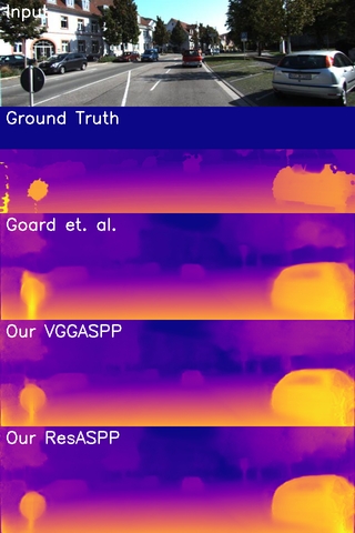
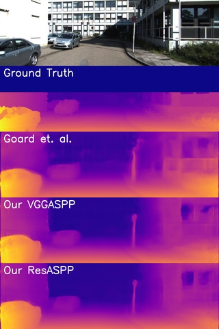
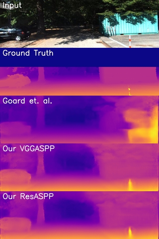
We include more quantitative results to further visualize the performance of our model on KITTI dataset. The proposed VGGASPP and ResASPP networks are both presented in all the results. In the network benchmark shown in Fig. 8, we use our prior [1] and [9] as the references without any post-processing to demonstrate the network performance. The performance is the same as that we have shown in the main manuscript. Our network can detect more objects clearly than state-of-the-art models, such as signs, poles, cars, etc. Comparing to our VGGASPP and ResASPP, the overall results are similar, but our ResASPP can get a few better prediction results on object shapes.

In the integration benchmark shown in Fig. 9, we only have one prior [1] as the reference due to the lack of the source information from other priors. We further showcase the ability to capture the clear object shapes with the minimal halo effects in our methods. We can produce very clear disparity images in the inference using the proposed Edge-Guided post-processing method.

Figure 8: More More qualitative results of network benchmark

Figure 9: More qualitative results of Integration benchmark

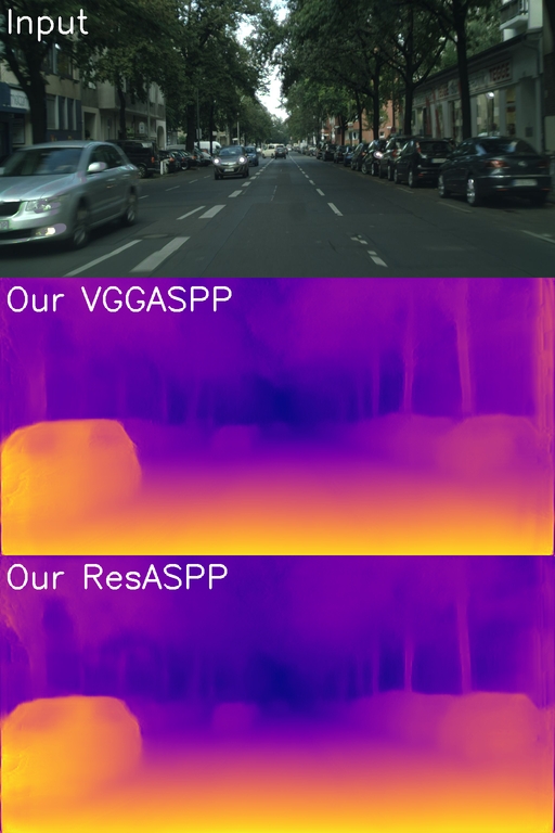
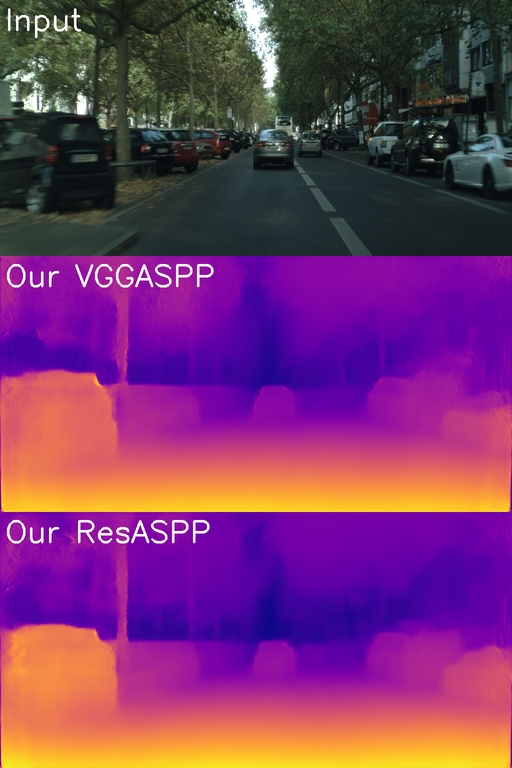
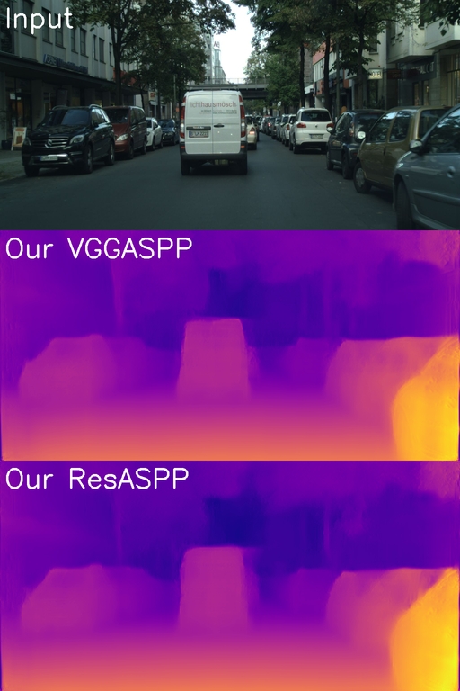
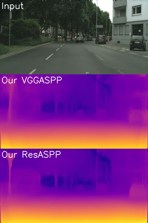
Appendix E Extended Results On More Datasets

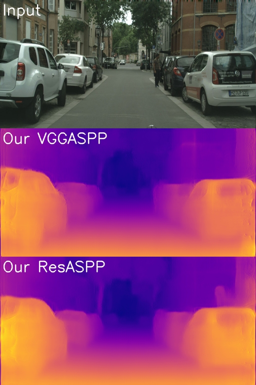
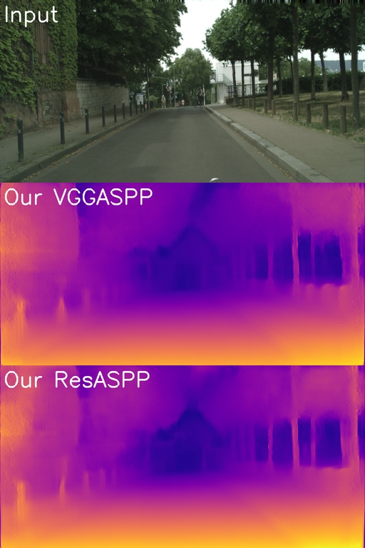
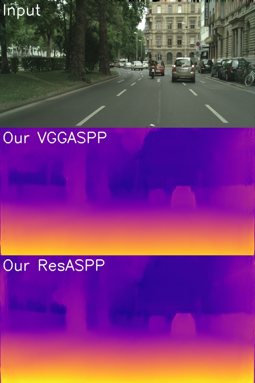
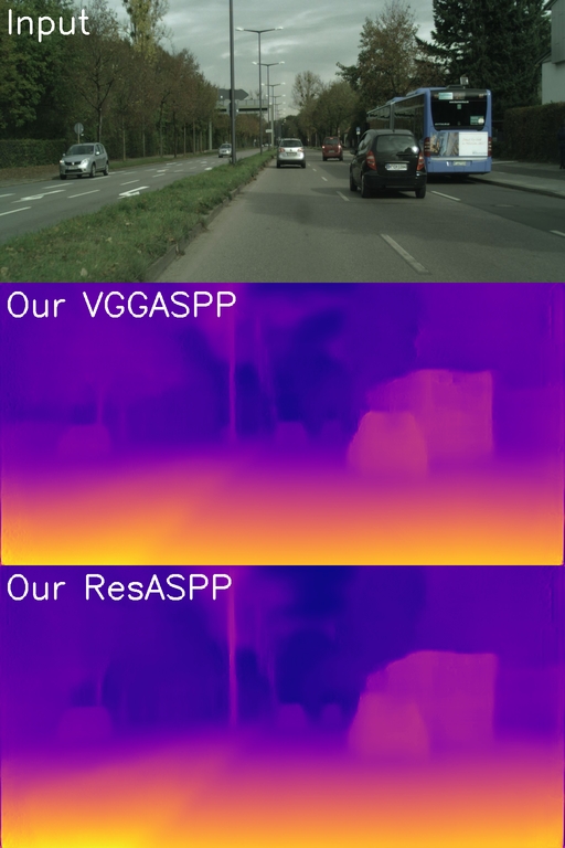
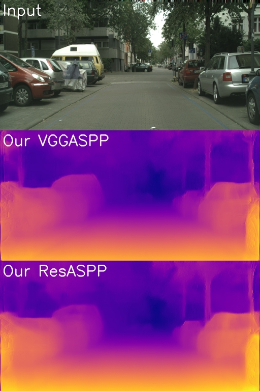
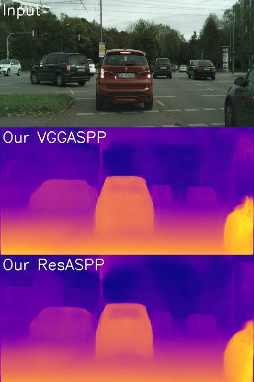
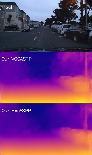
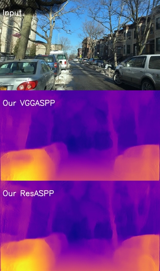
We extend our models to experiments on other datasets: Cityscapes [38] and Deepdrive [43]. Both these two datasets are outdoor scenes for the auto-driving application. We have used Cityscapes dataset as the pre-train dataset in the training process. We visualize the ten inference results in Fig. 10. The Deepdrive dataset is also designed for the auto-driving application with more different types of scenes. There are scenes in different weathers, and it is good for testing the model robustness. The original resolution of Deepdrive dataset is $720\times 1280$. We select another ten inference results of Deepdrive dataset shown in Fig. 11. The performance of the selected two datasets are consistent as the results on KITTI dataset. The proposed methods can finely capture the object shapes in the test images.

Figure 10: Cityscapes dataset qualitative results. There are 10 sets of images that we randomly select to show the visualization results.

Figure 11: Deepdrive dataset qualitative results. There are 10 sets of images that we randomly select to show the visualization results.

References

- [1] Clément Godard, Oisin Mac Aodha, and Gabriel Brostow. Unsupervised monocular depth estimation with left-right consistency. In Conference on Computer Vision and Pattern Recognition, 2017.
- [2] L Ladicky, J. Shi, and M. Pollefeys. Pulling things out of perspective. In Conference on Computer Vision and Pattern Recognition, 2014.
- [3] D Eigen, C Puhrsch, and R Fergus. Depth map prediction from a single image using a multi-scale deep network. In Advances in Neural Information Processing Systems, 2014.
- [4] F Liu, C Shen, G Lin, and I Reid. Learning depth from single monocular images using deep convolutional neural fields. IEEE Transactions on Pattern Analysis and Machine Intelligence, 38(10):2024–2039, 2016.
- [5] Max Jaderberg, Karen Simonyan, Andrew Zisserman, and Koray kavukcuoglu. Spatial transformer networks. In Advances in neural information processing systems, 2015.
- [6] Ting-Chun Wang, Manohar Srikanth, and Ravi Ramamoorthi. Depth from semi-calibrated stereo and defocus. In Proceedings of the IEEE Conference on Computer Vision and Pattern Recognition, pages 3717–3726, 2016.
- [7] David Eigen, Christian Puhrsch, and Rob Fergus. Depth map prediction from a single image using a multi-scale deep network. In Advances in neural information processing systems, pages 2366–2374, 2014.
- [8] Ravi Garg, Vijay Kumar, Gustavo Carneiro, and Ian Reid. Unsupervised cnn for single view depth estimation: Geometry to the rescue. In European Conference on Computer Vision, 2016.
- [9] Alex Wong and Stefano Soatto. Bilateral cyclic constraint and adaptive regularization for unsupervised monocular depth prediction. In Conference on Computer Vision and Pattern Recognition, 2019.
- [10] Hyowon Ha, Sunghoon Im, Jaesik Park, Hae-Gon Jeon, and In So Kweon. High-quality depth from uncalibrated small motion clip. In Proceedings of the IEEE Conference on Computer Vision and Pattern Recognition, pages 5413–5421, 2016.
- [11] Tinghui Zhou, Matthew Brown, Noah Snavely, and David G. Lowe. Unsupervised learning of depth and ego-motion from video. In IEEE Conference on Computer Vision and Pattern Recognition, 2017.
- [12] Sudheendra Vijayanarasimhan, Susanna Ricco, Cordelia Schmid, Rahul Sukthankar, and Katerina Fragkiadaki. Sfm-net: Learning of structure and motion from video. arXiv preprint, page 1704.07804, 2017.
- [13] Reza Mahjourian, Martin Wicke, and Anelia Angelova. Unsupervised learning of depth and ego-motion from monocular video using 3d geometric constraints. In IEEE Conference on Computer Vision and Pattern Recognition, 2018.
- [14] Zhichao Yin and Jianping Shi. Geonet: Unsupervised learning of dense depth, optical flow and camera pose. In IEEE Conference on Computer Vision and Pattern Recognition, 2018.
- [15] Huangying Zhan, Ravi Garg, Chamara Saroj Weerasekera, Kejie Li, Harsh Agarwal, and Ian Reid. Unsupervised learning of monocular depth estimation and visual odometry with deep feature reconstruction. In IEEE Conference on CVPR, 2018.
- [16] Kuo-Shiuan Peng, Gregory Ditzler, and Jerzy W. Rozenblit. Self-supervised correlational monocular depth estimation using resvgg network. In 7th IIAE International Conference on Intelligent Systems and Image Processing, pages 93–102, 2019.
- [17] Yevhen Kuznietsov, Jorg Stuckler, and Bastian Leibe. Semi-supervised deep learning for monocular depth map prediction. In Conference on Computer Vision and Pattern Recognition, 2017.
- [18] Ali Jahani Amiri, Shing Yan Loo, and Hong Zhang. Semi-supervised monocular depth estimation with left-right consistency using deep neural network. arXiv preprint, page 1905.07542, 2019.
- [19] Po-Yi Chen, Alexander H. Liu, Yen-Cheng Liu, and Yu-Chiang Frank Wang. Towards scene understanding: Unsupervised monocular depth estimation with semantic-aware representation. In Proceedings of the IEEE Conference on Computer Vision and Pattern Recognition, pages 2624–2632, 2019.
- [20] Lubor Ladicky, Jianbo Shi, and Marc Pollefeys. Pulling things out of perspective. In Proceedings of the IEEE conference on computer vision and pattern recognition, pages 89–96, 2014.
- [21] David Eigen and Rob Fergus. Predicting depth and surface normals and semantic labels with a common multi-scale convolutional architecture. In Proceedings of the IEEE international conference on computer vision, pages 2650–2658, 2015.
- [22] Peng Wang, Xiaohui Shen, Zhe Lin, Scott Cohen, Brian Price, and Alan L. Yuille. Towards unified depth and semantic prediction from a single image. In Proceedings of the IEEE Conference on Computer Vision and Pattern Recognition, pages 2800–2809, 2015.
- [23] Arsalan Mousavian, Hamed Pirsiavash, and Jana Košecká. Joint semantic segmentation and depth estimation with deep convolutional networks. In 2016 Fourth International Conference on 3D Vision, pages 611–619, 2016.
- [24] Jianbo Jiao, Ying Cao, Yibing Song, and Rynson Lau. Look deeper into depth: Monocular depth estimation with semantic booster and attention-driven loss. In Proceedings of the European Conference on Computer Vision, pages 53–69, 2018.
- [25] Pierluigi Zama Ramirez, Matteo Poggi, Fabio Tosi, Stefano Mattoccia, and Luigi Di Stefano. Geometry meets semantics for semi-supervised monocular depth estimation. In Asian Conference on Computer Vision, pages 298–313, 2018.
- [26] Zhenyu Zhang, Zhen Cui, Chunyan Xu, Zequn Jie, Xiang Li, and Jian Yang. Joint task-recursive learning for semantic segmentation and depth estimation. In Proceedings of the European Conference on Computer Vision, pages 235–251, 2018.
- [27] David J. Fleet Michael J. Black and Oscar Nestares. Bayesian inference of visual motion boundaries. Exploring Artificial Intelligence in the New Millennium, page 139, 2003.
- [28] Ahmad Hoiem, Derek, Alexei A. Efros, and Martial Hebert. Automatic photo pop-up. In ACM transactions on graphics, 24(3):577–584, 2005.
- [29] Ahmad Humayun, Oisin Mac Aodha, and Gabriel J. Brostow. Learning to find occlusion regions. In 2011 IEEE Computer Society Conference on Computer Vision and Pattern Recognition, pages 2161–2168, 2011.
- [30] Ang Li and Zejian Yuan. Symmnet: a symmetric convolutional neural network for occlusion detection. arXiv preprint, page 1807.00959, 2018.
- [31] Eddy Ilg, Tonmoy Saikia, Margret Keuper, and Thomas Brox. Occlusions and motion and depth boundaries with a generic network for disparity and optical flow or scene flow estimation. In Proceedings of the European Conference on Computer Vision, pages 614–630, 2018.
- [32] Vladimir Nekrasov, Chunhua Shen, and Ian Reid. Light-weight refinenet for real-time semantic segmentation. arXiv preprint, page 1810.03272, 2018.
- [33] Liang-Chieh Chen, George Papandreou, Florian Schroff, , and Hartwig Adam. Rethinking atrous convolution for semantic image segmentation. In arXiv preprint, page arXiv:1706.05587, 2017.
- [34] N Mayer, E Ilg, P Hausser, P Fischer, D Cremers, A Dosovitskiy, and T Brox. A large dataset to train convolutional networks for disparity, optical flow, and scene flow estimation. In Conference on Computer Vision and Pattern Recognition, 2016.
- [35] Vladimir Nekrasov, Thanuja Dharmasiri, Andrew Spek, Tom Drummond, Chunhua Shen, and Ian Reid. Real-time joint semantic segmentation and depth estimation using asymmetric annotations. In 2019 International Conference on Robotics and Automation, pages 7101–7107, 2019.
- [36] Liang-Chieh Chen, Yukun Zhu, George Papandreou, Florian Schroff, , and Hartwig Adam. Encoder-decoder with atrous separable convolution for semantic image segmentation. In In Proceedings of the European conference on computer vision, pages 801–818, 2018.
- [37] A Geiger, P Lenz, and R Urtasun. Are we ready for autonomous driving? the KITTI vision benchmark suite. In Conference on Computer Vision and Pattern Recognition, 2012.
- [38] Marius Cordts, Mohamed Omran, Sebastian Ramos, Timo Rehfeld, Markus Enzweiler, Rodrigo Benenson, Uwe Franke, Stefan Roth, and Bernt Schiele. The cityscapes dataset for semantic urban scene understanding. In IEEE conference on computer vision and pattern recognition, 2016.
- [39] M. Abadi et al. TensorFlow: Large-scale machine learning on heterogeneous systems, 2015.
- [40] Po-Yi Chen, Alexander H. Liu, Yen-Cheng Liu, and Yu-Chiang Frank Wang. Towards scene understanding: Unsupervised monocular depth estimation with semantic-aware representation. In Proceedings of the IEEE Conference on Computer Vision and Pattern Recognition, pages 2624–2632, 2019.
- [41] Clement Godard, Oisin Mac Aodha, and Gabriel Brostow. Digging into self-supervised monocular depth estimation. In arXiv:1806, 2018.
- [42] Myung-Kyu Han Dong Wook Ko Jin Han, Lee and Il Hong Suh. From big to small: Multi-scale local planar guidance for monocular depth estimation. arXiv preprint, page 1907.10326, 2019.
- [43] Fisher Yu, Wenqi Xian, Yingying Chen, Fangchen Liu, Mike Liao, Vashisht Madhavan, and Trevor Darrell. Bdd100k: A diverse driving video database with scalable annotation tooling. arXiv preprint, page 1805.04687, 2018.