Universal spectral features of different classes of random diffusivity processes

Abstract

Stochastic models based on random diffusivities, such as the diffusing-diffusivity approach, are popular concepts for the description of non-Gaussian diffusion in heterogeneous media. Studies of these models typically focus on the moments and the displacement probability density function. Here we develop the complementary power spectral description for a broad class of random diffusivity processes. In our approach we cater for typical single particle tracking data in which a small number of trajectories with finite duration are garnered. Apart from the diffusing-diffusivity model we study a range of previously unconsidered random diffusivity processes, for which we obtain exact forms of the probability density function. These new processes are different versions of jump processes as well as functionals of Brownian motion. The resulting behaviour subtly depends on the specific model details. Thus, the central part of the probability density function may be Gaussian or non-Gaussian, and the tails may assume Gaussian, exponential, log-normal or even power-law forms. For all these models we derive analytically the moment-generating function for the single-trajectory power spectral density. We establish the generic $1/f^{2}$-scaling of the power spectral density as function of frequency in all cases. Moreover, we establish the probability density for the amplitudes of the random power spectral density of individual trajectories. The latter functions reflect the very specific properties of the different random diffusivity models considered here. Our exact results are in excellent agreement with extensive numerical simulations.

7th March 2024

1 Introduction

Diffusive processes came to the attention of the broader scientific community with the experiments on "active molecules" by Robert Brown, who reported the jittery motion of granules of "1/4000th to 1/5000th of an inch in length" contained in pollen grains as well as control experiments on powdered inorganic rocks [1]. In the mid-19th century physician-physiologist Adolf Fick published his studies on salt fluxes between reservoirs of different concentrations connected by tubes [2]. To quantify the observed dynamics Fick introduced the diffusion equation ("Fick’s second law") for the spatio-temporal concentration profile. A major breakthrough was the theoretical description of "Brownian motion" and the diffusion equation in terms of probabilistic arguments by Einstein [3], Smoluchowski [4], and Sutherland [5]. Concurrently Karl Pearson introduced the notion of the "random walk" [6], and Langevin proposed the intuitive picture of the random force and the stochastic Langevin equation [7].

More recently, major advances in experimental techniques such as superresolution microscopy continue to provide unprecedented insight into the motion of submicron and even molecular tracers in complex environments such as living biological cells [8, 9, 10, 11]. Concurrently, simulations are becoming ever more powerful and reveal the Molecular Dynamics in systems such as lipid membranes [12] or internal protein motion [13]. The data resulting from such complex systems unveil a number of new phenomena in the stochastic particle motion and thus call for new theoretical concepts [14, 15, 16] on top of already known approaches [17, 18, 19].

Among these new insights is that endogenous and introduced tracers in living biological cells perform anomalous diffusion of the form $\langle\textbf{r}^{2}(t)\rangle\simeq K_{\alpha}t^{\alpha}$ in a wide range of systems [8, 9, 20]. For instance, subdiffusion with $0<\alpha<1$ was measured for messenger RNA probes in bacteria cells [21, 22], for DNA loci and telomeres in bacteria and eukaryotic cells [22, 23, 24], for granules in yeast and human cells [25, 26], as well as for the stochastic motion of biological membrane constituents [27, 28]. In these cases the slower than Brownian, passive tracer motion is effected by the highly crowded nature of the environment, as can be studied in in vitro systems [29, 30]. In fact, even small green fluorescent proteins of some 2 nanometre in size were shown to subdiffuse [31]. Conversely, superdiffusion with $1<\alpha<2$ in biological cells is caused by active motion of molecular motors due to consumption of biochemical energy units. Examples include the motor motion itself [32, 33], the transport of introduced plastic beads in fibroblast cells [34], RNA cargo in neuron cells [35], or of granules in amoeba [36].

However, even when the mean squared displacement seemingly suggests Brownian motion based on the observation that $\alpha=1$, remarkable effects have been reported recently. Thus, the motion of micron-sized tracer beads moving along nanotubes as well as in entangled polymer networks was shown to be "Fickian" yet the measured displacement distribution exhibited significant deviations from the expected Gaussian law: namely, an exponential distribution of the form $P(\mathbf{r},t)\propto\exp(-|\mathbf{r}|/\lambda(t))$ with $\lambda(t)\propto t^{1/2}$ was observed [37, 38]. Similar "Fickian yet non-Gaussian" diffusion was found for the tracer dynamics in hard sphere colloidal suspensions [39], for the stochastic motion of nanoparticles in nanopost arrays [40], of colloidal nanoparticles adsorbed at fluid interfaces [41, 42, 43] and moving along membranes and inside colloidal suspension [44], and for the motion of nematodes [45]. Even more complicated non-Gaussian distributions of displacements were recently observed in Dictyostelium discoideum cells [46, 47] and protein-crowded lipid bilayer membranes [48]. While in some experiments the non-Gaussian shape of $P(\mathbf{r},t)$ is observed over the entire experimental window, others report clear crossover behaviours from a non-Gaussian shape at shorter time scales to an effective Gaussian behaviour at longer time scales, for instance, see [37, 38].

A non-Gaussian probability density along with the scaling exponent $\alpha=1$ of the mean squared displacement can be achieved in the superstatistical approach, in which it is assumed that individual Gaussian densities are averaged over a distribution of diffusivities [49, 50, 51, 52, 53]. A microscopic realisation of such a behaviour was proposed for a model of diffusion during a polymerisation process [54]. However, in superstatistics (and in the related process called generalised grey Brownian motion [55, 56, 57]) the distribution is a constant of the motion and thus no crossover behaviour as mentioned above can be described. In order to include such a non-Gaussian to Gaussian crossover models were introduced in which the diffusion coefficient is considered as a stochastic process itself. In this diffusing-diffusivity picture, originally proposed by Chubynsky and Slater [58], the stochastic dynamics of the diffusivity is characterised by a well-defined correlation time above which the diffusivity becomes equilibrated. Concurrently to this equilibration the ensuing form of $P(\mathbf{r},t)$ becomes effectively Gaussian. Random diffusivity models have since then been developed and analysed further, and their application is mainly the diffusive dynamics in heterogeneous systems [59, 60, 61, 62, 63, 64, 65, 66, 67, 68, 69, 70].

In fact, stochastic models based on random diffusivities are ubiquitous in financial mathematics for the modelling of stock price. They are commonly known as stochastic volatility models and many different examples have been analysed in order to identify a proper description for the volatility [71]. Among them, one can find diffusion-based models, where the volatility is described with continuous sample paths, as well as more complicated dynamics where, for instance, jumps are also allowed or where the volatility is defined as a function of separate stochastic processes [72]. Financial mathematics hosts a rich variaty of random diffusivity models, motivated by various aspects of the observed financial market data. Here we present a range of additional, new random diffusivity models in the context of the time series analysis, generalising the diffusing-diffusivity model developed for Fickian yet non-Gaussian diffusion processes. As this field is quickly expanding and new facets are being continuously unveiled, we are confident that these different models and their features offer the necessary flexibility to account for these new observations.

The central purpose of our study here is twofold. First we analyse several new classes of random diffusivity models, divided into two groups, jump models and functionals of Brownian motion. For both groups we consider several concrete examples and derive analytic solutions for the probability density function (PDF) ${\bf{\bf\Pi}}(x,t)$. The PDF turns out to delicately depend on the precise formulation of the model: the central part may be Gaussian or non-Gaussian, and the tails may be of Gaussian, exponential, log-normal, or even power-law shape. The second goal we pursue here are the spectral properties of random diffusivity processes. Namely, while earlier studies of the random diffusivity dynamics were mainly concerned with the PDF and the mean squared displacement encoded in the process we assume a different stance and derive the the spectral properties of single particle trajectories with finite observation time, geared for the description of contemporary single particle tracking experiments. Such an analysis was worked out in detail for specific systems of normal and anomalous diffusion [73, 74, 75, 76, 77, 78], and we here study the commonalities and differences emerging for random diffusivity scenarios.

Traditionally, power spectral analyses are based on the textbook definition of the spectral density

$$\mu(f)=\lim_{T\to\infty}\frac{1}{T}\left\langle\left|\int_{0}^{T}e^{ift}x(t)dt\right|^{2}\right\rangle.$$ (1)

This definition involves taking the limit of infinite (practically, very long) measurement times as well as averaging over an ensemble (practically, a large number of) of particles, here and in the following denoted by angular brackets, $\langle\cdot\rangle$. Typical single particle tracking experiments, however, are limited in the measurement time, for instance, due to the lifetime of the employed fluorescent tags or the time a particle stays in the microscope focus. At the same time, such experiments are often limited to a relatively small number of individual trajectories. To cater for this common type of experimental situations we avoid taking the long time and ensemble limits by considering the single-trajectory power spectral density (PSD)

$$S_{T}(f)=\frac{1}{T}\left|\int_{0}^{T}e^{ift}x(t)dt\right|^{2}$$ (2)

as functions of frequency $f$ and measurement time $T$. We previously analysed the behaviour of $S(f,T)$ for different diffusion scenarios [76, 77, 78] and demonstrated that it is practically useful in the analysis of experimental data [76, 77]. In what follows we derive the moment-generating function (MGF) of the PSD (2) for different classes of random-diffusivity processes, including several cases not yet studied in literature. In particular, we obtain the probability density $P(A)$ of the single PSD amplitude, an intrinsically random quantity for a finite-time measurement of a stochastic motion that was demonstrated to be a very useful quantity for the analysis of measured particle trajectories. In addition to analytical derivations we present detailed numerical analyses. This study provides a quite general approach to obtain the PDF for any diffusing diffusivity model, providing new insights on this class of processes.

This work is structured as follows. We start from section 2 with a description of the model and in section 3 we report general results on the spectral properties of this class of processes. Specific examples of diffusing-diffusivity models are described in sections 4-6. The first example is the well known case in which the diffusivity is modelled as the squared Ornstein-Uhlenbeck process. In the second group of examples we analyse two cases in which the diffusivity is defined as a jump process. The third and last group shows three examples in which the diffusivity is described as a functional of Brownian motion. Finally, in section 7 we draw our conclusions. In the appendix we report details on the explicit derivations of our results.

2 Random diffusivity processes

We consider a class of one-dimensional stochastic processes $x_{t}$ that obey the Langevin equation in the Itô convention,

$$\dot{x}_{t}=\sqrt{2D_{0}\Psi_{t}}\xi_{t}.$$ (3)

Here $D_{0}$ is a constant, dimensional coefficient in units ${\rm length}^{2}/{\rm time}$, and in our analysis we will assume the initial condition $x_{0}=0$. In equation (3) $\xi_{t}$ denotes a standard Gaussian white noise with zero mean and covariance function $\overline{\xi_{t}\xi_{t^{\prime}}}=\delta\left(t-t^{\prime}\right)$. The bar here and henceforth denotes averaging with respect to the noise $\xi_{t}$. Lastly $\Psi_{t}$ is a positive-definite random function, which multiplies $D_{0}$ and thus introduces a time-dependent randomness into the effective noise amplitude. In the following we stipulate that $\Psi_{t}$ is Riemann-integrable on a finite interval $(0,T)$ such that $\int^{T}_{0}dt\Psi_{t}$ exists with probability $1$. Note that the case $\Psi_{t}\equiv 1$ corresponds to standard Brownian motion, while a deterministic choice of the form $\Psi_{t}=t^{\alpha-1}$ produces so-called scaled Brownian motion [79, 80]. We will here discuss several particular choices for the random function $\Psi_{t}$. In addition to the previously made choice of a squared Ornstein-Uhlenbeck process we will consider the case when $\Psi_{t}$ is a jump-process, that attains independent, identically distributed random values. We also present several examples when $\Psi_{t}$ is subordinated to standard unbiased Brownian motion $B_{t}$: namely, $\Psi_{t}=B^{2}_{t}/a^{2}$, where $a$ is a model parameter, $\Psi_{t}=\Theta(B_{t})$, where $\Theta(x)$ is the Heaviside theta function, and geometric Brownian motion $\Psi_{t}=\exp(-B_{t}/a)$.

Regardless of the choice of the random function $\Psi_{t}$, we can solve the Langevin equation (3) for the trajectory $x_{t}$ for a fixed realisation of the noise and a given realisation of $\Psi_{t}$, to obtain

$$x_{t}=(2D_{0})^{1/2}\int^{t}_{0}d\tau\Psi^{1/2}_{\tau}\xi_{\tau}.$$ (4)

The characteristic function of $x_{t}$ can be written down in the form

$$\Phi_{w}=\left<\overline{\exp\left(iw(2D_{0})^{1/2}\int^{t}_{0}d\tau\Psi^{1/2}_{\tau}\xi_{\tau}\right)}\right>_{\Psi},$$ (5)

where the bar stands for averaging over thermal histories, while the angular brackets denote averaging over the realisations of the random function $\Psi_{t}$. The thermal average can be performed straightforwardly to give

$$\Phi_{w}=\left<\exp\left(-D_{0}w^{2}\int^{t}_{0}d\tau\Psi_{\tau}\right)\right>_{\Psi}.$$ (6)

The desired PDF ${\bf\Pi}(x,t)$ can then be written as

$${\bf\Pi}(x,t)=\frac{1}{2\pi}\int^{\infty}_{-\infty}dwe^{-iwx}\Phi_{w}.$$ (7)

In the following section 4 we provide several examples with explicit expressions for the probability density, and we will see how different choices of $\Psi_{t}$ may lead to PDFs of considerably different shapes.

3 General theory

We first obtain exact expressions for the PSD (2) and then study the limiting behaviour for high frequencies.

3.1 Exact expressions for arbitrary frequency and observation time

We investigate the PSD of an individual trajectory $x_{t}$ encoded in the stochastic dynamics (3) with $t\in(0,T)$,

$$S_{T}(f)=\frac{1}{T}\int^{T}_{0}dt_{1}\int^{T}_{0}dt_{2}\cos\left(f(t_{1}-t_{2})\right)x_{t_{1}}x_{t_{2}},$$ (8)

as function of the frequency $f$ and the observation time $T$. We determine the MGF and the PDF of the random variable $S_{T}(f)$.

The MGF of the single-trajectory PSD in (8) is defined as

$$\phi_{\lambda}=\left<\overline{\exp\left(-\frac{\lambda}{T}\int^{T}_{0}dt\int^{T}_{0}dt^{\prime}\cos\left(f(t-t^{\prime})\right)x_{t}x_{t^{\prime}}\right)}\right>_{\Psi}$$ (9)

with $\lambda\geq 0$. Relegating some intermediate calculations to A we find the following expression for $\phi_{\lambda}$ in (9) averaged over thermal noises,

$$\phi_{\lambda} = \frac{1}{4\pi\lambda}\int^{\infty}_{-\infty}dz_{1}\int^{\infty}_{-\infty}dz_{2}\exp\left(-\frac{z_{1}^{2}+z_{2}^{2}}{4\lambda}\right)$$ (10)

$$\times\left\langle\exp\left(-D_{0}\int^{T}_{0}dt\Psi_{t}\left(\int^{T}_{t}d\tau Q_{\tau}\right)^{2}\right)\right\rangle_{\Psi},$$

where

$$Q_{t}=z_{1}\frac{\cos(ft)}{\sqrt{T}}+z_{2}\frac{\sin(ft)}{\sqrt{T}}.$$ (11)

Performing the inverse Laplace transform of expression (10), we find the general result for the PDF

$$p(S_{T}(f)=S) = \displaystyle\frac{1}{4\pi}\int^{\infty}_{-\infty}dz_{1}\int^{\infty}_{-\infty}dz_{2}J_{0}\left(\sqrt{\left(z_{1}^{2}+z_{2}^{2}\right)S}\right)$$ (12)

$$\times\left\langle\exp\left(-D_{0}\int^{T}_{0}dt\Psi_{t}\left(\int^{T}_{t}d\tau Q_{\tau}\right)^{2}\right)\right\rangle_{\Psi},$$

where $J_{0}(z)$ denotes the Bessel function of the first kind. A more explicit dependence on the frequency $f$ can be obtained in the form (see A for more details)

$$\phi_{\lambda} = \Bigg{\langle}\Bigg{[}1+\frac{8\lambda D_{0}}{f^{2}T}\int^{T}_{0}dt\Psi_{t}\bigg{(}1-\cos\left(f\left(T-t\right)\right)\bigg{)}$$ (13)

$$+\frac{16\lambda^{2}D_{0}^{2}}{f^{4}T^{2}}\int^{T}_{0}dt_{1}\Psi_{t_{1}}\int^{T}_{0}dt_{2}\Psi_{t_{2}}\left(\frac{3}{4}+L_{f}(t_{1},t_{2})\right)\Bigg{]}^{-1/2}\Bigg{\rangle}_{\Psi},$$

where $L_{f}(t_{1},t_{2})$ is defined by the somewhat lengthy expression (103).

The expression within the angular brackets in relation (13) is the exact MGF of the PSD of the process $x_{t}$ in (3) for any fixed realisation of $\Psi_{t}$ and holds for arbitrary $T$ and arbitrary $f$. It also represents the exact form of the MGF in the case when $\Psi_{t}$ is non-fluctuating: in particular, for $\Psi_{t}=1$ it describes the MGF in case of standard Brownian motion [76], while the choice $\Psi_{t}=t^{\alpha-1}$ corresponds to the case of scaled Brownian motion recently studied in [78].

3.2 Exact high frequency limiting behaviour

As already remarked we here concentrate on random processes $\Psi_{t}$ which, for any finite $T$, are Riemann-integrable with probability $1$, which implies that in the limit $f\to\infty$ certain integrals vanish, as shown in B. As a consequence, expression (13) attains the following exact analytic high-frequency form

$$\phi_{\lambda}\sim\Bigg{\langle}\Bigg{[}1+\frac{8\lambda D_{0}}{f^{2}T}\int^{T}_{0}dt\Psi_{t}+\frac{12\lambda^{2}D_{0}^{2}}{f^{4}T^{2}}\left(\int^{T}_{0}dt\,\Psi_{t}\right)^{2}\Bigg{]}^{-1/2}\Bigg{\rangle}_{\Psi},$$ (14)

in which we dropped the vanishing terms and kept only the leading terms in $1/f$.

We note that the Laplace parameter $\lambda$ appears in the combination $D_{0}\lambda/f^{2}$ so that the high-$f$ spectrum of a single-trajectory PSD has the universal form

$$S_{T}(f)\sim\frac{4D_{0}A}{f^{2}},$$ (15)

regardless of the specific choice of $\Psi_{t}$. Here $A$ is a dimensionless, random amplitude, which differs from realisation to realisation. This means that the characteristic high-frequency dependence of the PSD can be learned, in principle, from just a single trajectory, in agreement with the conclusions in [76, 77, 78].

The MGF $\Phi_{\lambda}$ of the random amplitude $A$ follows from (14) and can be written as

$$\Phi_{\lambda} = \int\limits_{0}^{\infty}dAe^{-\lambda A}P(A)$$ (16)

$$= \frac{2}{\sqrt{3}}\int^{\infty}_{0}dp\exp\left(-\frac{4p}{3}\right)I_{0}\left(\frac{2p}{3}\right)\Upsilon(T;\lambda p/T),$$

where $I_{0}(z)$ is the modified Bessel function of the first kind, and

$$\Upsilon(T;\lambda)=\Bigg{\langle}\exp\left(-\lambda\int^{T}_{0}dt\Psi_{t}\right)\Bigg{\rangle}_{\Psi}$$ (17)

is the MGF of the integrated diffusivity (see [64, 66])

$$\tau_{T}=\int\nolimits_{0}^{T}dt\Psi_{t}.$$ (18)

Relation (16) links the MGFs of $A$ and $\tau_{T}$. Moreover, note that the characteristic function of the diffusing-diffusivity model in (6) is tightly related to the MGF of $\tau_{T}$ in (17), specifically

$$\Upsilon(T;D_{0}w^{2})=\Phi_{w}.$$ (19)

As shown in [64] the function $\Upsilon(T;\lambda)$ determines the first-passage time properties of the stochastic process $x_{t}$. Here we show how this function controls the high-frequency behaviour of the PSD.

Taking the inverse Laplace transform with respect to the parameter $\lambda$ we evaluate the PDF of $A$,

$$P(A) = \frac{2}{\sqrt{3}}\int^{\infty}_{0}dzJ_{0}\left(\left(1+\frac{1}{\sqrt{3}}\right)\sqrt{2zA}\right)$$ (20)

$$\times J_{0}\left(\left(1-\frac{1}{\sqrt{3}}\right)\sqrt{2zA}\right)\Upsilon(T;z/T).$$

This exact expression determines the high-$f$ behaviour of the PDF $p(S_{T}(f)=S)$,

$$p(S_{T}(f)=S)\sim\frac{f^{2}}{4D_{0}}P\left(A=\frac{Sf^{2}}{4D_{0}}\right)$$ (21)

as $f\to\infty$. The exact high-$f$ forms in (16) and (20) will serve as the basis of our analysis for several particular choices of the process $\Psi_{t}$ in section 4.

Before proceeding, we stop to make several general statements.

(i) Expanding the exponential function on the right hand side of (16) into the Taylor series in powers of $\lambda$ we obtain straightforwardly the relation between the moments of $A$ and the moments of the integrated diffusivity $\tau_{T}$, which is valid for any $n$,

$${\mathbb{E}}\{A^{n}\}=\left(\frac{3}{4}\right)^{n+1/2}n!{{}_{2}F_{1}}\left(\frac{n+1}{2},\frac{n+2}{2};1;\frac{1}{4}\right)\left\langle\frac{\tau_{T}^{n}}{T^{n}}\right\rangle_{\Psi},$$ (22)

where ${}_{2}F_{1}(a,b;c;z)$ is the Gauss hypergeometric function. Since the moments of $\tau_{T}$ are related to the moments of the process $x_{T}$ [66] we also find

$${\mathbb{E}}\{A^{n}\}=\left(\frac{3}{4}\right)^{n+1/2}\frac{(n!)^{2}}{(2n)!}\,_{2}F_{1}\left(\frac{n+1}{2},\frac{n+2}{2};1;\frac{1}{4}\right)\\ \left\langle\frac{x_{T}^{2n}}{(D_{0}T)^{n}}\right\rangle_{\Psi}.$$ (23)

(ii) Starting from the results in (22) and (23) we can readily obtain the moments of $S_{T}(f)$ as well. In particular, if we focus on its average value, we have

$$\langle S_{T}(f)\rangle=\frac{4D_{0}C_{1}}{f^{2}T}\langle\tau_{T}\rangle_{\Psi}=\frac{2C_{1}}{f^{2}T}\left\langle\overline{x_{T}^{2}}\right\rangle_{\Psi},$$ (24)

where $C_{1}={(3/4)^{3/2}}_{2}F_{1}(1,3/2;1;1/4)$. This suggests that those random diffusivity models that display anomalous scaling of the MSD, i.e., $\left\langle\overline{x_{T}^{2}}\right\rangle_{\Psi}\not\simeq T$, exhibit ageing behaviour, namely, a dependence of the PSD properties on the trajectory length $T$.

(iii) Equations (15) and (22) permit us to directly access the coefficient of variation $\gamma$ of the PDF $p(S_{T}(f)=S)$ in the high-$f$ limit. We get straightforwardly

$$\gamma = \left(\frac{\left\langle\overline{S_{T}^{2}(f)}\right\rangle_{\Psi}-\left\langle\overline{S_{T}(f)}\right\rangle^{2}_{\Psi}}{\left\langle\overline{S_{T}(f)}\right\rangle^{2}_{\Psi}}\right)^{1/2}\approx\left(\frac{\left\langle A^{2}\right\rangle_{\Psi}-\left\langle A\right\rangle^{2}_{\Psi}}{\left\langle A\right\rangle^{2}_{\Psi}}\right)^{1/2}$$ (25)

$$= \left(\frac{3}{4}\frac{\left\langle x^{4}_{T}\right\rangle_{\Psi}}{\left\langle x^{2}_{T}\right\rangle^{2}_{\Psi}}-1\right)^{1/2}=\left(\frac{9}{4}\frac{\left\langle\tau^{2}_{T}\right\rangle_{\Psi}}{\left\langle\tau_{T}\right\rangle^{2}_{\Psi}}-1\right)^{1/2}$$

$$= \left(\frac{9}{4}\frac{\partial^{2}_{\lambda}\Upsilon(T;\lambda)|_{\lambda=0}}{\left(\partial_{\lambda}\Upsilon(T;\lambda)|_{\lambda=0}\right)^{2}}-1\right)^{1/2},$$

which implies that the effective broadness of $p(S_{T}(f)=S)$ is entirely defined by the first two moments of the random variable $\tau_{T}$ in (18). Specifically, it is independent of $D_{0}$ and $f$ when $f$ is only large enough.

(iv) The behaviour of the left tail of $p(S_{T}(f)=S)$ can be assessed in the following way. Note that the product of the two Bessel functions in (20) can be represented as a power series with an infinite radius of convergence (see (106) in C). Inserting the expansion in (106) in (20) and integrating over $z$ we find

$$\quad P(A)=\frac{2}{\sqrt{3}}\sum_{n=0}^{\infty}\frac{(-1)^{n}}{n!}\left(\frac{\sqrt{3}+1}{\sqrt{6}}\right)^{2n}{{}_{2}F_{1}}\left(-n,-n;1;\frac{1-\sqrt{3}/2}{1+\sqrt{3}/2}\right)\left\langle\frac{T^{n+1}}{\tau_{T}^{n+1}}\right\rangle_{\Psi}A^{n},$$ (26)

if the inverse moments of the variable $\tau_{T}$ exist (and do not grow too fast with $n$). Therefore, the PDF $P(A)$ is an analytic function of $A$ in the vicinity of $A=0$, with

$$P(0)=\frac{2}{\sqrt{3}}\left\langle\frac{T}{\tau_{T}}\right\rangle_{\Psi}.$$ (27)

We note that below we will encounter both situations when $P(A)$ is analytic and when it is not. In the latter situation we will show that $p(S_{T}(f)=S)$ diverges as $S\to 0$, which can be already inferred from (27).

4 Diffusivity modelled as squared Ornstein-Uhlenbeck process

In this and the following sections we apply the above general theory to several random diffusivity models. According to our main results (16) and (20) one first needs to evaluate the MGF $\Upsilon(T;\lambda)$ of the integrated diffusivity $\tau_{T}$ for a chosen diffusivity process $\Psi_{t}$. To illustrate the quality of the theoretical predictions in the high-frequency limit we also performed numerical simulations using a Python code. The Euler integration scheme is used to compute (3), where $\Psi_{t}$ is obtained by a numerical integration of the proper stochastic equation for each case. The PSD is obtained by fast Fourier transform for each trajectory. Starting from the single-trajectory power spectra the random amplitude $A$ is calculated according to (15).

Concretely when $\Psi_{t}$ in the diffusing-diffusivity model is defined as a stochastic process satisfying some Langevin equation, the distribution of $A$ is determined by (16) and (20) through the MGF $\Upsilon(T;\lambda)$ of the integrated diffusivity $\tau_{T}$ that can be obtained by solving the associated backward Fokker-Planck equation (see [66] for details). Here we consider the common example of squared Ornstein-Uhlenbeck process and related models. We note that diffusing-diffusivity models are intimately related to random-coefficient autoregressive processes [81].

The Ornstein-Uhlenbeck process $Y_{t}$

$$\dot{Y}_{t}=-\tau_{\star}^{-1}Y_{t}+\sigma_{\star}\xi^{\prime}_{t}$$ (28)

is a stationary Gaussian process mean-reverting to zero at a time scale $\tau_{\star}$ and driven by standard Gaussian white noise $\xi^{\prime}_{t}$ with volatility $\sigma_{\star}$. The process $\Psi_{t}=Y_{t}^{2}$ is one of the most common models of diffusing diffusivity, which satisfies, due to the Itô’s formula,

$$\dot{\Psi}_{t}=\tau^{-1}(\bar{\Psi}-\Psi_{t})+\sigma\sqrt{2\Psi_{t}}\xi^{\prime}_{t},$$ (29)

where $\tau=\tau_{\star}/2$, $\sigma=\sqrt{2}\sigma_{\star}$, and $\bar{\Psi}=\sigma_{\star}^{2}\tau_{\star}/2=\sigma^{2}\tau/2$. This model was extended in [59, 60, 61] by considering $\Psi_{t}$ as the sum of $n$ independent squared Ornstein-Uhlenbeck processes, when (29) still holds with $\bar{\Psi}=n\sigma^{2}\tau/2$. More generally, setting $\bar{\Psi}$ to be any positive constant, the Langevin equation (29) defines the so-called Feller process [82], also known as square root process or the Cox-Ingersoll-Ross process [83], also used in the Heston model [84] . This process was used to model the diffusing-diffusivity in [63, 64], see also the discussion in [61].

Figure 1: Diffusing-diffusivity defined as the squared Ornstein-Uhlenbeck process, for three different values of $\tau_{\star}$. Other parameters are $T=10^{2}$ and $\sigma_{\star}=1$. Panels a)-c) show a few realisations of the power spectra from individual trajectories and the average value for $\tau_{\star}=10^{0},10^{1},10^{2}$, respectively. Panel d) shows a comparison of the mean power spectrum. Panel e) shows the coefficient of variation, the black dashed lines correspond to the theoretical result in (31). Panel f) shows the distribution of the random amplitude $A$, the black dashed lines correspond to (20) with the explicit expression of the MGF from (30).

The MGF $\Upsilon(T;\lambda)$ for the integrated squared Ornstein-Uhlenbeck process was first computed by Dankel [85] and employed in [59, 60, 61]. Its computation for the Feller process in (29) was presented in [63],

$$\Upsilon(T;\lambda)=\left(\frac{4\omega e^{-(\omega-1)T/(2\tau)}}{(\omega+1)^{2}-(\omega-1)^{2}e^{-\omega T/\tau}}\right)^{\nu},$$ (30)

where $\omega=\sqrt{1+4\sigma^{2}\tau^{2}\lambda}$ and $\nu=\bar{\Psi}/(\tau\sigma^{2})$. In particular, setting $\bar{\Psi}=\sigma^{2}\tau/2$ (and thus $\nu=1/2$) one retrieves the MGF for the squared Ornstein-Uhlenbeck process. A detailed discussion on the PDF of this model is presented in [59, 60, 61, 63, 64]. Using the explicit formulas for $\left\langle\overline{x_{T}^{2}}\right\rangle_{P}si$ and $\left\langle\overline{x_{T}^{4}}\right\rangle_{\Psi}$ from [61, 63] we get from (25) that

$$\gamma=\left[\frac{3}{4}\left(3+\frac{6\tau}{\nu T}\left(1-\frac{\tau}{T}(1-e^{-T/\tau})\right)\right)-1\right]^{1/2}.$$ (31)

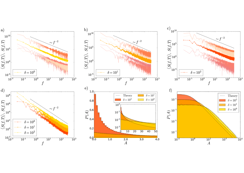
Moreover, as the second moment $\langle\overline{x_{T}^{2}}\rangle$ shows a linear trend in time [61, 63], no ageing of the PSD occurs, as suggested in (24).

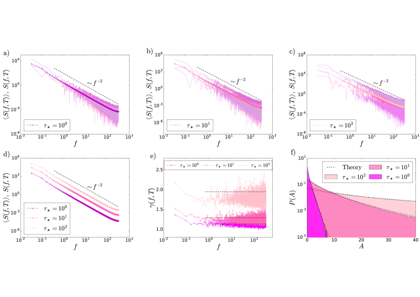
The PDF of $A$ is determined via (20). Since an explicit calculation of this integral is not straightforward we perform a numerical integration. The results are shown in Fig. 1, in which we observe excellent agreement between the simulations and the theoretical results. The $1/f^{2}$ scaling is recovered for any value of $\tau_{\star}$. The coefficient of variation $\gamma$ converges to different values when we change $\tau_{\star}$, according to (31). Note that this result reflects the different degrees of broadness of the PDF of the random amplitude $A$. In particular for $\tau_{\star}\ll T$ we obtain a result that is very similar to the one of Brownian motion, while for increasing $\tau_{\star}$ the PDF of the random amplitude $A$ becomes increasingly broader.

5 Diffusivity modelled as a jump process

We divide the interval $(0,T)$ into $N$ equal subintervals of duration $\delta=T/N$ and suppose that $\Psi_{t}$ is a jump process on these intervals, of the form

$$\Psi_{t}=\psi_{k}\mbox{ on }t\in\bigl{(}[k-1]\delta,k\delta\bigr{)},\quad k=1,\ldots,N.$$ (32)

Furthermore we stipulate that the $\psi_{k}$ are independent, identically distributed, positive-definite random variables with PDF $\rho(\psi)$. In other words, we take that $\Psi_{t}$ at each discrete time instant $(k-1)\delta$ attains a new random value, taken from the common distribution, and stays constant and equal to this value up to the next discrete instant $k\delta$. For a given realisation of the process $\Psi_{t}$ we thus have

$$\tau_{T}=\int^{T}_{0}dt\Psi_{t}=\delta\sum_{k=1}^{N}\psi_{k},$$ (33)

and hence

$$\Upsilon(T;\lambda)=\left(\int^{\infty}_{0}d\psi\rho(\psi)e^{-\lambda\delta\psi}\right)^{T/\delta}.$$ (34)

Evaluating explicitly the derivatives $\partial_{\lambda}\Upsilon(T;\lambda)$ and $\partial^{2}_{\lambda}\Upsilon(T;\lambda)$ at $\lambda=0$, we get

$$\langle\tau_{T}\rangle=T\,{\mathbb{E}}\{\psi_{k}\},$$ (35)

when the first moment ${\mathbb{E}}\{\psi_{k}\}$ exists. From this we infer $\left\langle\overline{x_{T}^{2}}\right\rangle_{\Psi}$ and thus the respective ageing behaviour. Moreover, the coefficient of variation becomes

$$\gamma=\left[\frac{9}{4}\left(1-\frac{\delta}{T}+\frac{\delta}{T}\frac{{\mathbb{E}}\{\psi_{k}^{2}\}}{{\mathbb{E}}\{\psi_{k}\}^{2}}\right)-1\right]^{1/2},$$ (36)

when the first two moments ${\mathbb{E}}\{\psi_{k}\}$ and ${\mathbb{E}}\{\psi_{k}^{2}\}$ exist.

Modelling the diffusivity as a jump process can be seen as a way to describe the model in section 4 through a different parametrisation. Indeed, we define a time scale, which is given by the duration $\delta$ of each step interval, and we then introduce a random variability of the diffusivity from one interval to the next. These diffusivity fluctuations are chosen according to the PDF $\rho(\psi)$. Of course, the main difference comes form the fact that in this model we do not have any correlation between successive diffusivities. In what follows we analyse two examples in detail. In the first one we select a Gamma distribution for $\rho(\psi)$, in analogy with the diffusing-diffusivity model in section 4, where the diffusion coefficient shows a Gamma distribution as well. In the second example we select a Lévy-Smirnov distribution for $\rho(\psi)$. This allows us to model a system in which a high probability of having small values of the diffusivity is combined with the presence of few outliers, which can be related, for instance, to values of the diffusivity at boundaries of the system.

Figure 2: Position-PDF at a fixed time $t=50$ for diffusivity modelled as a jump process with Gamma distribution ($\psi_{0}=1$ and $\nu=0.5$). Panels a) and c) correspond to $\delta=1$, and panels b) and d) to $\delta=100$. Panels a) and b) show a comparison between the numerical and the analytic result in (39) (black dashed lines). Panel c) shows a comparison between the analytic result (39) for $\delta=1$ and its Gaussian approximation (51). Panel d) compares between the analytical result (39) for $\delta=100$ and its asymptotic behaviours in (43) and (44).

5.1 Example I: Gamma distribution

Figure 3: Diffusivity modelled as a jump process with Gamma distribution ($\psi_{0}=1$ and $\nu=0.5$), for varying $\delta$ and with trajectory length $T=10^{2}$. Panels a)-c) show a few realisations of the power spectra from individual trajectories and the mean value for $\delta=10^{2}$, $5\times 10^{1}$, and $10^{0}$, respectively. Panel d) shows the coefficient of variation for three values of $\delta$—the black dashed lines represent the theoretical result (36). Panels e)-f) depict the distribution of the random amplitude $A$ in linear, semi-log (inset) and log-log scale. Here the black dashed line corresponds to the theoretical result (50).

First, we consider the Gamma distribution,

$$\rho(\psi)=\frac{\psi^{\nu-1}}{\Gamma(\nu)\psi_{0}^{\nu}}\exp\left(-\psi/\psi_{0}\right)$$ (37)

with the shape parameter $\nu>0$ and the scale parameter $\psi_{0}>0$. From (34), we deduce

$$\Upsilon(T;\lambda)=\left(1+\lambda\delta\psi_{0}\right)^{-\nu T/\delta}.$$ (38)

Position-PDF ${\bf\Pi}(x,t)$

A direct calculation of the PDF for this model can be performed. Starting from (7) and recalling that $\Phi_{w}=\Upsilon(T;D_{0}w^{2})$, we get

$${\bf\Pi}(x,t)={\cal N}_{t}\left(\frac{|x|}{2\sqrt{D_{0}\delta\psi_{0}}}\right)^{\frac{\nu t}{\delta}-\frac{1}{2}}K_{\frac{1}{2}-\frac{\nu t}{\delta}}\left(\frac{|x|}{\sqrt{D_{0}\delta\psi_{0}}}\right),$$ (39)

where the normalisation coefficient is

$${\cal N}_{t}=\sqrt{\frac{2}{\pi}}\Big{/}\left(\left(D_{0}\delta\psi_{0}\right)^{3/4}\Gamma\left(\frac{\nu t}{\delta}\right)\right).$$ (40)

With the properties

$$z^{\nu}K_{-\nu}(z)\sim 2^{\nu-1}\Gamma(\nu)-\frac{2^{\nu-3}\Gamma(\nu)}{\nu-1}z^{2}$$ (41)

for $|z|\to 0$ and $\nu>1$, as well as

$$K_{-\nu}\sim\sqrt{\frac{\pi}{2z}}e^{-z}$$ (42)

for $|z|\to\infty$, the asymptotic behaviours of the PDF are given by

$${\bf\Pi}(x,t)\sim{\cal N}_{t}\,2^{\frac{\nu t}{\delta}-\frac{3}{2}}\Gamma\left(\frac{\nu t}{\delta}-\frac{1}{2}\right)\left[1-\frac{x^{2}}{4\left(\frac{\nu t}{\delta}-\frac{3}{2}\right)D_{0}\delta\psi_{0}}\right]$$ (43)

for $|x|\to 0$ and $\nu t>3\delta/2$, as well as

$${\bf\Pi}(x,t)\sim\frac{2}{\sqrt{D_{0}\delta\psi_{0}}\Gamma\left(\frac{\nu t}{\delta}\right)}\left(\frac{|x|}{2\sqrt{D_{0}\delta\psi_{0}}}\right)^{\frac{\nu t}{\delta}-1}\exp\left(-\frac{|x|}{\sqrt{D_{0}\delta\psi_{0}}}\right)$$ (44)

for $|x|\to\infty$.

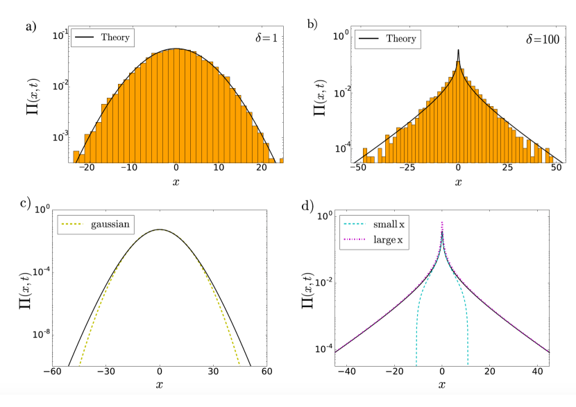
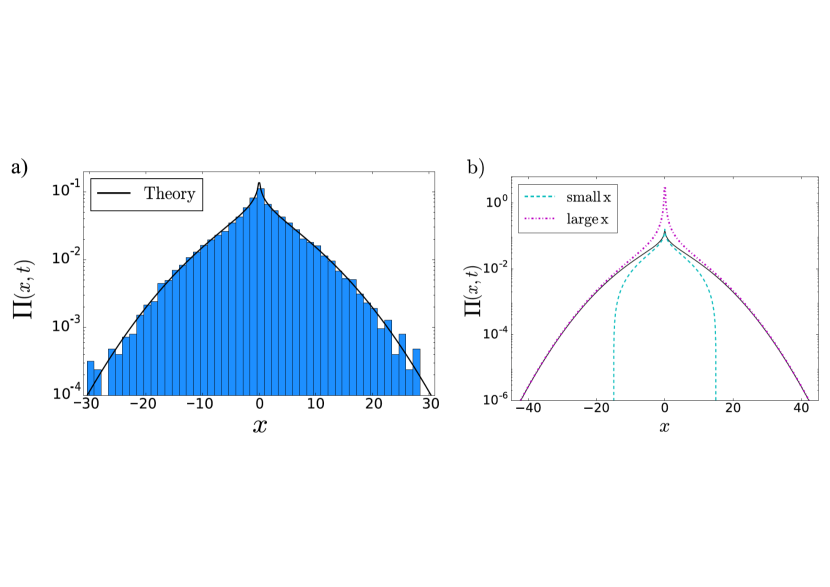
The functional behaviour of the PDF ${\bf\Pi}(x,t)$ is shown in Fig. 2. We see that by changing $\delta$ we can observe different shapes of ${\bf\Pi}(x,t)$. When $\delta=1$ (panels a) and c)) the Gaussian approximation (51) already provides a good estimate of the PDF over a wide range. We start observing discrepancies only far out in the tails, for values which can hardly be reached with real data. When $\delta=100$ (panels b) and d)), in contrast, the exponential tails are distinct. The behaviours at small and large $x$ are well described by the asymptotic expansions in (43) and (44). Note that the value of $\delta$ in here plays a role similar to the correlation time $\tau_{\star}$ in the diffusing-diffusivity model defined in section 4. The only difference is that by changing $\tau_{\star}$ in the model above we also change the average diffusivity while, in this case, changes in the value of $\delta$ do not affect the average diffusivity, which is fixed once we choose the jumps PDF in (37).

Amplitude-PDF $P(A)$

The MGF of the amplitude $A$ of the jump process-diffusivity model is given by

$$\Phi_{\lambda}=\frac{2}{\sqrt{3}}\int^{\infty}_{0}dp\frac{\displaystyle\exp\left(-4p/3\right)I_{0}(2p/3)}{\displaystyle\left(1+p\psi_{0}\lambda\delta/T\right)^{\nu T/\delta}},$$ (45)

so that

$$\qquad P(A)=\frac{2}{\sqrt{3}}\int^{\infty}_{0}dz\frac{\displaystyle J_{0}\left(\left(1+1/\sqrt{3}\right)\sqrt{2zA}\right)}{\displaystyle\left(1+z\psi_{0}\delta/T\right)^{\nu T/\delta}}J_{0}\left(\left(1-1/\sqrt{3}\right)\sqrt{2zA}\right).$$ (46)

In particular one has ${\mathbb{E}}\{\psi_{k}\}=\nu\Psi_{0}$ and ${\mathbb{E}}\{\psi_{k}^{2}\}=\Psi_{0}^{2}\nu(\nu+1)$, thus from (35) we readily obtain $\left\langle\overline{x_{T}^{2}}\right\rangle_{\Psi}\simeq T$, demonstrating that in this process no ageing behaviour is displayed. Moreover, from (36) we get

$$\gamma=\left[\frac{9}{4}\left(1+\frac{\delta}{\nu T}\right)-1\right]^{1/2}.$$ (47)

In the limit $\delta\to 0$ and $N\to\infty$, with $\delta N=T$ fixed, we have

$$\Upsilon(T;\lambda)\sim\exp\left(-\nu\psi_{0}T\lambda\right).$$ (48)

Hence,

$$\Phi_{\lambda} = \frac{2}{\sqrt{3}}\int^{\infty}_{0}dp\exp\left(-\left(\frac{4}{3}+\nu\psi_{0}\lambda\right)p\right)I_{0}\left(\frac{2p}{3}\right)$$ (49)

$$= \left(1+2\nu\psi_{0}\lambda+\frac{\displaystyle 4}{\displaystyle 3}(\nu\psi_{0}\lambda)^{2}\right)^{-1/2}$$

and

$$\qquad P(A) = \frac{2}{\sqrt{3}}\int^{\infty}_{0}dzJ_{0}\left(\left(1+1/\sqrt{3}\right)\sqrt{2zA}\right)J_{0}\left(\left(1-1/\sqrt{3}\right)\sqrt{2zA}\right)e^{-\nu\psi_{0}z}$$ (50)

$$= \frac{2}{\sqrt{3}\nu\psi_{0}}\exp\left(-\frac{4A}{3\nu\psi_{0}}\right)I_{0}\left(\frac{2A}{3\nu\psi_{0}}\right).$$

This means that we have essentially the same behaviour as for standard one-dimensional Brownian motion, however, with renormalised coefficients (compare with the result in [76]), in agreement also with what we obtained for the diffusing-diffusivity model in section 4, when selecting $\tau_{\star}\ll T$. Indeed, if we use (48) and recall that $\Phi_{w}=\Upsilon(T;D_{0}w^{2})$, we readily obtain

$${\bf\Pi}(x,t)\sim\frac{1}{2\sqrt{\pi\nu\psi_{0}D_{0}t}}\exp\left(-\frac{x^{2}}{4\nu\psi_{0}D_{0}t}\right).$$ (51)

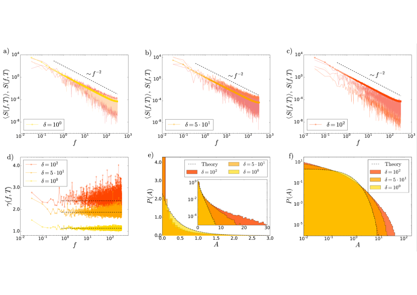
In Fig. 3 we show a direct comparison between the numerical and theoretical results for the Gamma distribution with $\psi_{0}=1$ and $\nu=0.5$. We observe that the average value of the power spectrum is not affected by the value of $\delta$. Nevertheless, when we plot some sample single-trajectory power spectra we notice a larger amplitude scatter for larger values of $\delta$. This may be clearly seen in the distribution of the random variable $A$, which is broader for larger values of $\delta$, and consequently in the different limiting values of the coefficient of variation. Thus, the fluctuations are sensitive to different parameters of the distribution (37), while the mean behaviour is not.

5.2 Example II: Lévy-Smirnov distribution

In our second example we consider the Lévy-Smirnov distribution

$$\rho(\psi)=\sqrt{\frac{\displaystyle\psi_{0}}{\displaystyle\pi}}\frac{\displaystyle\exp\left(-\psi_{0}/\psi\right)}{\displaystyle\psi^{3/2}},$$ (52)

for which Eq. (34) yields

$$\Upsilon(T;\lambda)=\exp\left(-2T\sqrt{\psi_{0}\lambda/\delta}\right).$$ (53)

Note that in this case ${\mathbb{E}}\{\psi_{k}\}$ and ${\mathbb{E}}\{\psi_{k}^{2}\}$ are not defined, such that $\left\langle\overline{x_{T}^{2}}\right\rangle_{\Psi}$ does not exist either. This suggests that a clear ageing behaviour cannot be defined and that fluctuations are what dominates the system.

Position-PDF ${\bf\Pi}(x,t)$

As a consequence, we obtain the following analytical expression for the PDF,

$${\bf\Pi}(x,t)=\frac{2t\sqrt{D_{0}\psi_{0}/\delta}}{\pi}\frac{1}{4t^{2}D_{0}\psi_{0}/\delta+x^{2}},$$ (54)

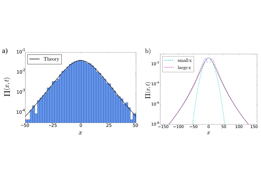
where we recognise the power-law behaviour, that is already built into relation (52). Note that expression (54) represents the Cauchy distribution, whose median grows with time $t$.

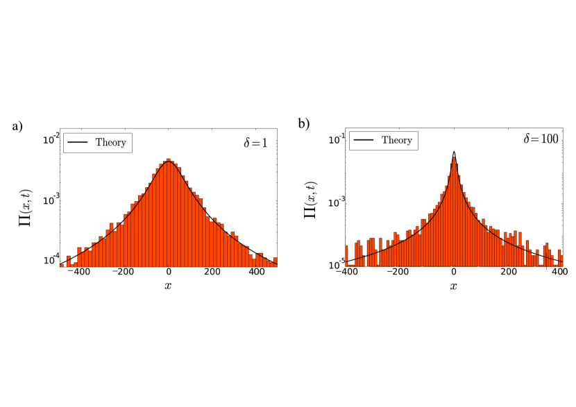
The PDF is shown for two different values of $\delta$ in Fig. 4. We observe that, differently from the case with the Gamma distribution above, we do not see significant changes in the shape of the distribution when varying $\delta$. For both cases, $\delta=1$ and $\delta=100$, the power-law behaviour (54) is readily discernible.

Figure 4: Position-PDF at fixed time $t=50$ for diffusivity modelled as a jump process with Lévy-Smirnov distribution, $\Psi_{0}=0.5$, for a) $\delta=1$ and b) $\delta=100$. The black dashed line represents the analytical result (54).

Amplitude-PDF $P(A)$

Figure 5: Diffusivity modelled as a jump process with Lévy-Smirnov distribution with $\psi_{0}=0.5$, for varying $\delta$ and with trajectory length $T=10^{2}$. Panels a)-c) show a few realisations of the power spectra from individual trajectories and the mean value for $\delta=10^{2}$, $10^{1}$, and $10^{0}$, respectively. Panel d) compares the mean values of the power spectrum. Panels e)-f) show the distribution of the random amplitude $A$ in linear, semi-log (inset) and log-log scale—the black dashed line corresponds to the analytical result (56).

The MGF for the random amplitude $A$ reads

$$\Phi_{\lambda}=\frac{2}{\sqrt{3}}\int^{\infty}_{0}dp\exp\left(-\frac{4}{3}p-2\sqrt{p\psi_{0}\lambda T/\delta}\right)I_{0}\left(\frac{2p}{3}\right)$$ (55)

and

$$P(A) = \frac{2}{\sqrt{3}}\int^{\infty}_{0}dzJ_{0}\left(\left(1+1/\sqrt{3}\right)\sqrt{2zA}\right)$$ (56)

$$\times J_{0}\left(\left(1-1/\sqrt{3}\right)\sqrt{2zA}\right)\exp\left(-2\sqrt{z\psi_{0}T/\delta}\right)$$

$$= \frac{\delta}{\sqrt{3}\psi_{0}T}\frac{1}{(1+\xi)^{3/2}}\,_{2}F_{1}\left(\frac{3}{4},\frac{5}{4};1;\frac{\xi^{2}}{4(1+\xi)^{2}}\right),$$

with $\xi=(4A\delta)/(3\psi_{0}T)$. Note that in the limit $A\to\infty$, the leading behaviour of $P(A)$ follows

$$P(A)\sim\frac{1}{A^{3/2}}.$$ (57)

Thus, the PDF $P(A)$ inherits the property of diverging moments from the parental Lévy-Smirnov distribution.

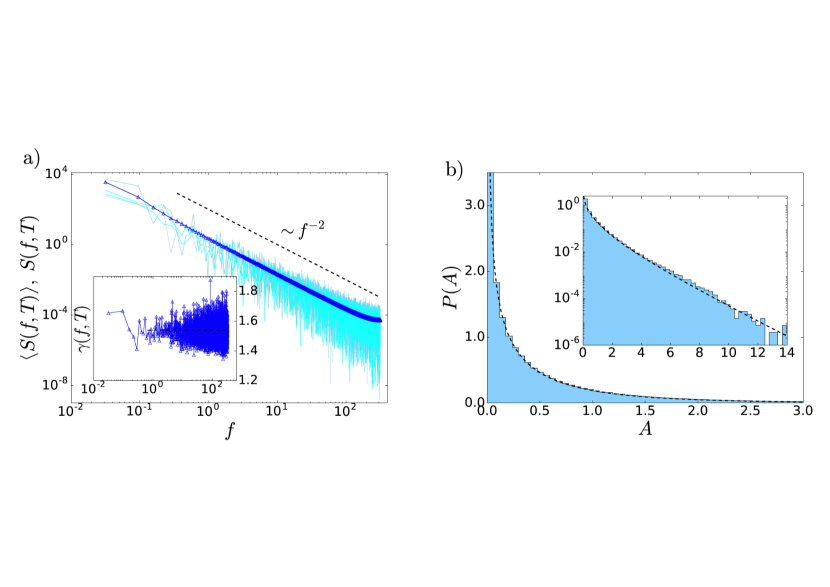
Figure 5 summarises the properties of the PSD for the jump process with Lévy-Smirnov distribution ($\psi_{0}=0.5$). We observe that, despite the fat-tailed PDF in (54) we still observe the universal $1/f^{2}$ scaling of the PDF. Concurrently, the PDF of the random amplitude $A$ features the power-law behaviour according to (56). Note that the non-existence of the moments of $P(A)$ generates a pronounced scatter in the amplitude of the average power spectrum.

6 Diffusivity modelled as a functional of Brownian motion

We now focus on the case when $\Psi_{t}$ is a genuine "diffusing-diffusivity" in the sense that it is subordinated to Brownian motion $B_{t}$ starting at the origin at $t=0$, with zero mean and covariance function

$$\left\langle B_{t}B_{t^{\prime}}\right\rangle=2D_{B}\min\{t,t^{\prime}\}.$$ (58)

We here choose $\Psi_{t}=V[B_{t}]$, where $V$ is some prescribed, positive-definite function. Note that random variables of the form $\int^{T}_{0}dtV[B_{t}]$ appear across many disciplines, including probability theory, statistical analysis, computer science, mathematical finance and physics. Starting from earlier works [89, 90, 91, 92, 93], much effort has been invested in the analysis of the PDF and the corresponding Laplace transforms of these processes. A large body of exact results has been obtained within the last seven decades (see, e.g., [94, 95, 96, 97, 98, 99] and further references therein). In the following, we consider three particular examples of $V[B_{t}]$, for which we can carry out exact calculations and obtain insightful results.

6.1 Example I: $\Psi_{t}=\Theta(B_{t})$

First, we choose the cut-off Brownian motion

$$\Psi_{t}=\Theta(B_{t}),$$ (59)

where $\Theta(x)$ is the Heaviside theta function. The process $x_{t}$ exhibits standard diffusive motion, once $B_{t}>0$, and pauses, remaining at the position it has reached when $B_{t}$ goes to negative values. The random variable $\int^{T}_{0}dt\Psi_{t}$ defines the time spent by a Brownian trajectory, starting at the origin, on the positive real line within the time interval $(0,T)$. The time intervals between any two "diffusion tours", as well as their duration, are random variables with a broad distribution.

This example is of particular interest as it represents an alternative to other standard models describing waiting times and trapping events. One could think, for instance, of the comb model, where a particle, while performing standard Brownian motion along one direction, gets stuck for a random time in branches perpendicular to the direction of the diffusive motion [100, 101].

The MSD of the process $x_{t}$, as one can straightforwardly check, is just

$$\left\langle\overline{x_{t}^{2}}\right\rangle_{\Psi}=D_{0}t,$$ (60)

that is, a standard diffusion law in which the diffusion coefficient is reduced by the factor $1/2$. This means that no ageing behaviour is observed. For higher order moments one expects, of course, significant departures from the standard diffusive behaviour.

Figure 6: Position-PDF at fixed time $t=50$ for diffusivity modelled as Heaviside function of Brownian motion, with $D_{B}=1$. Panel a) compares the numerical results with the analytical expression (62) (black solid line). Panel b) shows a comparison between the analytical result and its asymptotic behaviours (63) and (64).

Position-PDF ${\bf\Pi}(x,t)$

The MGF of the random variable $\tau_{T}=\int^{T}_{0}dt\Theta(B_{t})$, which has a bounded support on $(0,T)$, has been first derived by Kac [91], and Erdös and Kac [92]. Rewriting their result in our notation we have

$$\Upsilon(T;\lambda) = \Bigg{\langle}\exp\left(-\lambda\int^{T}_{0}dt\Theta(B_{t})\right)\Bigg{\rangle}_{\Psi}$$ (61)

$$= e^{-\lambda T/2}I_{0}\left(\frac{\lambda T}{2}\right).$$

Note that the inverse Laplace transform of this expression produces the celebrated Lévy arcsine law [102]. With result (61), the desired PDF is given by

$${\bf\Pi}(x,t) = \frac{1}{\pi}\int^{\infty}_{0}dw\cos(wx)\exp\left(-\frac{D_{0}t}{2}w^{2}\right)I_{0}\left(\frac{D_{0}t}{2}w^{2}\right)$$ (62)

$$= \frac{\exp\left(-x^{2}/(8D_{0}t)\right)}{2\sqrt{\pi^{3}D_{0}t}}K_{0}\left(\frac{x^{2}}{8D_{0}t}\right).$$

Recalling that $K_{0}(z)\sim-\ln(z/2)-\gamma_{\mathrm{EM}}$ for $|z|\to 0$, where $\gamma_{\mathrm{EM}}$ is the Euler-Mascheroni constant, for small $x$ we have

$${\bf\Pi}(x,t)\sim\frac{-\ln\left(\frac{x^{2}}{8D_{0}t}\right)-\gamma_{\mathrm{EM}}}{2\sqrt{\pi^{3}D_{0}t}},\quad|x|\to 0.$$ (63)

For large $x$ we use (42) and obtain the asymptotic behaviour for the PDF,

$${\bf\Pi}(x,t)\sim\frac{1}{\pi|x|}\exp\left(-\frac{x^{2}}{4D_{0}t}\right),\quad|x|\to\infty.$$ (64)

The PDF for this process is shown in Fig. 6. We see that the central part of the PDF is strongly non-Gaussian, while the tails are Gaussian, in agreement with the asymptotic behaviours (63) and (64).

Amplitude-PDF $P(A)$

Inserting expression (61) into (16) and performing the integration over $z$, we arrive at the following, remarkably compact expression for the MGF,

$$\Phi_{\lambda}=\frac{2\sqrt{2}}{\pi\sqrt{2+3\lambda}}{\bf K}\left(\frac{2\lambda}{2+3\lambda}\right)$$ (65)

where ${\bf K}(x)$ is the complete elliptic integral of the first kind,

$${\bf K}(x)=\int^{\pi/2}_{0}\frac{d\phi}{\sqrt{1-x\sin^{2}(\phi)}}.$$ (66)

Note that the high-$f$ asymptotic form in (65) is independent of the observation time $T$.

To proceed we take advantage of the definition of the complete elliptic integral and perform the inverse Laplace transform of (65). After some formal manipulations this yields the following expression for the PDF,

$$\qquad P\left(A\right)=2\sqrt{\frac{2}{3\pi^{3}A}}\int^{\pi/2}_{0}\frac{\displaystyle d\phi}{\displaystyle\sqrt{1-\frac{2}{3}\sin^{2}(\phi)}}\exp\left(-\frac{\displaystyle 2A}{\displaystyle 3\left(1-\frac{2}{3}\sin^{2}(\phi)\right)}\right).$$ (67)

Multiplying both sides of the latter equation by $A^{n}$ and integrating over $A$ from $0$ to $\infty$, we get the following simple expression for the moments of the random amplitude $A$ of an arbitrary order,

$${\mathbb{E}}\{A^{n}\}=\frac{\displaystyle\Gamma\left(n+\frac{1}{2}\right)}{\displaystyle\sqrt{\pi}}\left(\frac{\displaystyle 3}{\displaystyle 2}\right)^{n}\,_{2}F_{1}\left(-n,\frac{1}{2};1;\frac{2}{3}\right).$$ (68)

Then, from (25), we readily get the coefficient of variation, $\gamma=\sqrt{19/8}$.

Note that the integrals $\int^{\infty}_{0}d\lambda\lambda^{n}\Upsilon(T;\lambda)$ diverge for any $n>0$, which means that $\tau_{T}$ does not have negative moments. One therefore expects that $P(A)$ is a non-analytic, diverging function in the limit $A\to 0$. The small-$A$ asymptotic behaviour of $P(A)$ can be deduced directly from (67). Expanding the exponential function in the integral into the Taylor series in powers of $A$ and expressing the emerging generalised elliptic integrals via their representations in terms of the toroidal functions $P_{n-1/2}\left(\cosh(\eta)\right)$ (see (108) in C), we get

$$P\left(A\right)=\sqrt{\frac{2}{\sqrt{3}\pi A}}\sum_{n=0}^{\infty}\frac{(-1)^{n}}{n!}\left(\frac{2}{\sqrt{3}}\right)^{n}P_{n-1/2}\left(\frac{2}{\sqrt{3}}\right)A^{n}.$$ (69)

For the opposite limit $A\to\infty$, we conveniently rewrite Eq. (56) in the form

$$\qquad P(A) = 2\sqrt{\frac{2}{3\pi^{3}A}}\exp\left(-\frac{2A}{3}\right)\int^{\pi/2}_{0}\frac{d\phi}{\sqrt{\left(1-\frac{2}{3}\sin^{2}(\phi)\right)}}\exp\left(-\frac{2A}{3}\frac{\frac{2}{3}\sin^{2}(\phi)}{1-\frac{2}{3}\sin^{2}(\phi)}\right)$$ (70)

$$= 2\sqrt{\frac{2}{3\pi^{3}A}}\exp\left(-\frac{2A}{3}\right)\sum_{n=0}^{\infty}\left(\int^{\pi/2}_{0}\sin^{2n}(\phi)\right)\left(\frac{2}{3}\right)^{n}{\rm L}^{(-1/2)}_{n}\left(\frac{2A}{3}\right)$$

$$= \frac{2}{3\pi}\sqrt{\frac{3}{2A}}\exp\left(-\frac{2A}{3}\right)\sum_{n=0}^{\infty}\frac{\Gamma(n+1/2)}{n!}\left(\frac{2}{3}\right)^{n}{\rm L}^{(-1/2)}_{n}\left(\frac{2A}{3}\right),$$

where ${\rm L}^{(-1/2)}_{n}(x)$ are associated Laguerre polynomials. We focus next on the asymptotic behaviour of the function

$$g(u)=u^{-1/2}\sum_{n=0}^{\infty}\frac{\Gamma(n+1/2)}{n!}\left(\frac{2}{3}\right)^{n}{\rm L}^{(-1/2)}_{n}\left(u\right)$$ (71)

in the limit $u\to\infty$. Performing a Laplace transform of $g(u)$ we readily get

$${\cal L}_{s}\left\{g(u)\right\} = \int^{\infty}_{0}du\exp\left(-su\right)g(u)$$ (72)

$$= \frac{1}{s^{1/2}}\sum_{n=0}^{\infty}\frac{\Gamma^{2}(n+1/2)}{(n!)^{2}}\left(\frac{2(s-1)}{3s}\right)^{n}$$

$$= \frac{2}{s^{1/2}}{\bf K}\left(\frac{2(s-1)}{3s}\right),$$

where ${\bf K}$ is the complete elliptic integral defined in Eq. (66). In the limit $s\to 0$ (corresponding to $A\to\infty$),

$${\cal L}_{s}\left\{g(u)\right\}\sim\frac{2}{s^{1/2}}{\bf K}\left(-\frac{2}{3s}\right)=2\int^{\pi/2}_{0}\frac{d\phi}{\sqrt{s+\frac{2}{3}\sin^{2}(\phi)}}.$$ (73)

Inverting the Laplace transform and integrating over $\phi$, we find

$$g(u)\sim\frac{\pi}{\sqrt{u}}\exp\left(-\frac{u}{3}\right)I_{0}\left(\frac{u}{3}\right)\to\sqrt{\frac{3}{2}}\frac{1}{u}.$$ (74)

Thus, in the limit $A\to\infty$, the leading behaviour of the PDF $P(A)$ yields in the form

$$P(A)\sim\frac{1}{\pi A}\sqrt{\frac{3}{2}}\exp\left(-\frac{2A}{3}\right).$$ (75)

Figure 7 summarises the numerical results for this case. Again we observe excellent agreement with the theoretical results.

Figure 7: Diffusivity modelled as Heaviside theta function of Brownian motion, with $D_{B}=1$ and trajectory length $T=10^{2}$. Panel a) shows the mean power spectrum along with a few realisations of power spectra from individual trajectories. In the inset the coefficient of variation is shown, the black dashed line indicates the theoretical value $\sqrt{19/8}\approx 1.54$. Panel b) shows the distribution of the random amplitude $A$. Here the black dashed line corresponds to the numerical evaluation of (67).

6.2 Example II: $\Psi_{t}=\exp(-B_{t}/a)$.

As the second example, we link the process $\Psi_{t}$ to so-called geometric Brownian motion. Random variables of this form have been widely studied in the mathematical finance literature (see, e.g., [94]). Within the latter domain, they emerge very naturally as representation of the solution of the celebrated Black-Scholes equation. Their time-averaged counterpart is related to the so-called Asian options [103, 104, 105] (see also [106, 107]) and also appears in different contexts in the analysis of transport phenomena in disordered media (see, e.g., [108, 109, 110, 111, 112, 113, 114]) as well as characterises some features of the melting transition of heteropolymers [115].

In our notation, we set

$$\Psi_{t}=\exp\left(-\frac{B_{t}}{a}\right),$$ (76)

where $a$ is a parameter of unit length. In this case, $x_{t}$ exhibits an anomalously strong superdiffusion such that

$$\left\langle\overline{x_{t}^{2}}\right\rangle = 2D_{0}\int^{t}_{0}d\tau\langle\Psi_{\tau}\rangle_{\Psi}=2D_{0}\int^{t}_{0}d\tau\exp\left(D_{B}\tau/a^{2}\right)$$ (77)

$$= \frac{2D_{0}a^{2}}{D_{B}}\left(\exp\left(D_{B}t/a^{2}\right)-1\right).$$

Note that when $D_{B}t/a^{2}\ll 1$ we have $\left\langle\overline{x_{t}^{2}}\right\rangle\sim 2D_{0}t$. These results for the MSD demonstrate that for this model, in general, we observe ageing behaviour, though the latter may be hidden while analysing very short trajectories.

Position-PDF ${\bf\Pi}(x,t)$

The Laplace transform of the time-averaged geometric Brownian motion in our notation reads [109, 110, 111]

$$\Upsilon(T;\lambda) = \Bigg{\langle}\exp\left(-\lambda\int^{T}_{0}dt\exp\left(-\frac{B_{t}}{a}\right)\right)\Bigg{\rangle}_{\Psi}$$ (78)

$$= \frac{2a}{\sqrt{\pi D_{B}T}}\int^{\infty}_{0}dx\exp\left(-\frac{a^{2}x^{2}}{D_{B}T}\right)\cos\left(2a\sqrt{\frac{\lambda}{D_{B}}}\sinh(x)\right)$$

$$= \frac{2}{\pi}\int^{\infty}_{0}dx\exp\left(-\frac{D_{B}T}{4a^{2}}x^{2}\right)\cosh\left(\frac{\pi x}{2}\right)K_{ix}\left(2a\sqrt{\frac{\lambda}{D_{B}}}\right),$$

where $K_{ix}$ is the modified Bessel function of the second kind with purely imaginary index. As a consequence, the PDF is given by

$${\bf\Pi}(x,t) = \left(\frac{2}{\pi}\right)^{3/2}\int^{\infty}_{0}dz\exp\left(-\frac{D_{B}t}{4a^{2}}z^{2}\right)\cosh\left(\frac{\pi z}{2}\right)$$ (79)

$$\times\int^{\infty}_{0}dw\cos(wx)K_{iz}\left(2a|w|\sqrt{\frac{D_{0}}{D_{B}}}\right)$$

$$= \frac{1}{2\sqrt{\pi b_{2}t(b_{1}^{2}+x^{2})}}\exp\left(-\frac{{\rm arcsinh}^{2}(x/b_{1})}{4b_{2}t}\right),$$

where

$$b_{1}=2a\sqrt{\frac{D_{0}}{D_{B}}},\quad b_{2}=\frac{D_{B}}{4a^{2}}.$$ (80)

Recalling that ${\rm arcsinh}(z)\sim z$ for $z\to 0$ and ${\rm arcsinh}(z)\sim\ln(2z)$ for $z\to\infty$, we express the asymptotic behaviour of the PDF as

$${\bf\Pi}(x,t)\sim\frac{1}{2\sqrt{\pi b_{2}t(b_{1}^{2}+x^{2})}}\exp\left(-\frac{x^{2}}{4b_{2}tb_{1}^{2}}\right)$$ (81)

for $|x|\to 0$ and

$${\bf\Pi}(x,t)\sim\frac{1}{2\sqrt{\pi b_{2}t(b_{1}^{2}+x^{2})}}\exp\left(-\frac{\ln^{2}(2x/b_{1})}{4b_{2}t}\right)$$ (82)

for $|x|\to\infty$.

The PDF is shown in Fig. 8. In this case, according to the asymptotic expansions (81) and (82) we observe that the central part of the PDF is approximately Gaussian, while the tails follow a log-normal shape.

Amplitude-PDF $P(A)$

Figure 8: PDF at time $t=50$ for diffusivity modelled as geometric Brownian motion, with $D_{B}=1$ and $a=10$. Panel a) compares the numerical result and the analytical expression (79) (black solid line). Panel b) shows a comparison between the analytical result and its asymptotic behaviours (81) and (82).

Figure 9: Diffusivity modelled as geometric Brownian motion, with $D_{B}=1$, $a=10$, and trajectory length $T=10^{2}$. Panel a) shows the mean power spectrum and a few realisations of the power spectra from individual trajectories. In the inset the coefficient of variation is shown—the black dashed line corresponds to the theoretical result (83). Panel b) shows the distribution of the random amplitude $A$. Here the black dashed line corresponds to the numerical evaluation of (20), by making use of (78) also.

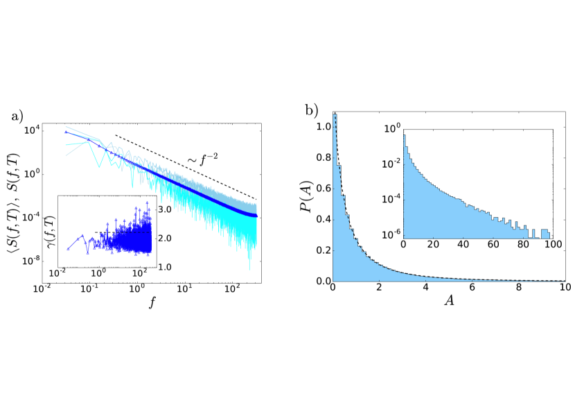
Evaluating explicitly $\partial_{\lambda}\Upsilon(T;\lambda)$ and $\partial^{2}_{\lambda}\Upsilon(T;\lambda)$ at $\lambda=0$, we get

$$\gamma=\left[\frac{3}{8}\left(3+e^{D_{B}T/a^{2}}\left(2+e^{D_{B}T/a^{2}}\right)\right)-1\right]^{1/2}.$$ (83)

Figure 9 summarises our numerical results, which show excellent agreement with the theoretical prediction.

6.3 Example III: $\Psi_{t}=B_{t}^{2}/a^{2}$

Finally, we consider squared Brownian motion

$$\Psi_{t}=\frac{B_{t}^{2}}{a^{2}},$$ (84)

where $a$ is a parameter of unit length. Note that here the process $x_{t}$ in (3) is superdffusive, such that its mean-squared displacement obeys

$$\left\langle\overline{x_{t}^{2}}\right\rangle_{\Psi}=\frac{2D_{0}D_{B}}{a^{2}}t^{2},$$ (85)

and thus a pronounced ageing behaviour occurs.

This example, similarly to the diffusing-diffusivity model in section 4, defines the diffusivity as the squared of an auxiliary variable, though in this case the variable follows a Brownian motion instead of the OU process. This choice implies that there is no crossover time, in contrast to the standard diffusing-diffusivity model, and thus we obtain a model which is always non-stationary. In particular, we introduce a larger separation between small and large values of the diffusivity, which may be interpreted as non-linear effects of the heterogeneity. Note that, if we were to define a random duration $\delta$ of the intervals, this model could be linked to a correlated CTRW [86, 87].

Position-PDF ${\bf\Pi}(x,t)$

The Laplace transform of the PDF of integrated squared Brownian motion was first calculated in the classical paper by Cameron and Martin [89, 90] (see also [91]). In our notation,

$$\Upsilon(T;\lambda) = \left\langle\exp\left(-\frac{\lambda}{a^{2}}\int^{T}_{0}dtB_{t}^{2}\right)\right\rangle_{\Psi}$$ (86)

$$= \frac{\displaystyle 1}{\displaystyle\sqrt{\cosh\left(\sqrt{4D_{B}T^{2}\lambda/a^{2}}\right)}},$$

and the PDF ${\bf\Pi}(x,t)$ for this process is given by

$${\bf\Pi}(x,t) = \frac{1}{\pi}\int^{\infty}_{0}\frac{dw\cos\left(wx\right)}{\sqrt{\cosh\left(w\sqrt{4D_{B}D_{0}t^{2}/a^{2}}\right)}}$$ (87)

$$= \frac{1}{\sqrt{2}ct}{\rm sech}\left(\frac{\pi x}{ct}\right)P_{\frac{ix}{ct}-\frac{1}{2}}\left(0\right),$$

where $c=2\sqrt{D_{0}D_{B}}/a$ and $P_{\nu}(z)$ is the Legendre function of the first kind. The latter admits the representation

$$P_{ix/ct-1/2}(0)=\sqrt{\pi}\Big{/}\left[\Gamma\left(\frac{ix}{2ct}+\frac{3}{4}\right)\Gamma\left(-\frac{ix}{2ct}+\frac{3}{4}\right)\right],$$ (88)

such that

$${\bf\Pi}(x,t)=\frac{\sqrt{\pi}}{ct\sqrt{2}}\frac{{\rm sech}(\frac{\pi x}{ct})}{\Gamma\left(\frac{ix}{2ct}+\frac{3}{4}\right)\Gamma\left(-\frac{ix}{2ct}+\frac{3}{4}\right)}.$$ (89)

In the limits,

$$\Gamma\left(\frac{ix}{2ct}+\frac{3}{4}\right)\Gamma\left(-\frac{ix}{2ct}+\frac{3}{4}\right)\sim\Gamma\left(\frac{3}{4}\right)^{2}$$ (90)

for $|x|\to 0$, and

$$\Gamma\left(\frac{ix}{2ct}+\frac{3}{4}\right)\Gamma\left(-\frac{ix}{2ct}+\frac{3}{4}\right)\sim\pi\sqrt{\frac{2|x|}{ct}}\exp\left(-\frac{\pi|x|}{2ct}\right)$$ (91)

for $|x|\to\infty$. As a consequence, the behaviour of the PDF for small $x$ is approximately Gaussian, $\simeq\exp(-\mathrm{const.}x^{2})$, where $\mathrm{const.}$ is a constant that can be expressed via the polylogarithm function. Conversely,

$${\bf\Pi}(x,t)\sim\frac{1}{\pi ct|x|}\exp\left(-\frac{\pi|x|}{2ct}\right)$$ (92)

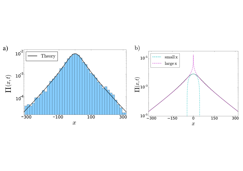
for $|x|\to\infty$. The shape of the PDF is shown in Fig. 10. We clearly observe that the central part is approximately Gaussian while the tails have an exponential trend, as expressed explicitly by the asymptote (92).

Figure 10: Position-PDF at fixed time $t=50$ for diffusivity modelled as squared Brownian motion, with $D_{B}=1$ and $a=1$. Panel a) compares between the numerical result and expression (87) (black solid line). Panel b) shows a comparison between the analytical result and its asymptotic behaviour (92) and the small $x$ behaviour of ${\rm sech}(z)$ form discussed in the text.

Figure 11: Diffusivity modelled as squared Brownian motion, with $D_{B}=1$, $a=1$, and trajectory length $T=10^{2}$. Panel a) shows the mean power spectrum along with a few realisations of power spectra from individual trajectories. In the inset the coefficient of variation is displayed—the black dashed line indicates the theoretical value $\sqrt{17}/2\approx 2.06$. Panel b) shows the distribution of the random amplitude $A$. Here the black dashed line corresponds to the numerical evaluation of (94).

Amplitude-PDF $P(A)$

Using (86) we then find that the MGF of the random amplitude $A$ and the corresponding PDF are given by the integrals

$$\Phi_{\lambda}(A)=\frac{2}{\sqrt{3}}\int^{\infty}_{0}dp\frac{\displaystyle\exp\left(-4p/3\right)I_{0}(2p/3)}{\displaystyle\sqrt{\cosh\left(\sqrt{4D_{B}T\lambda p/a^{2}}\right)}}$$ (93)

and

$$P(A)=\frac{2}{\sqrt{3}}\int^{\infty}_{0}dz\frac{\displaystyle J_{0}\left((1+1/\sqrt{3})\sqrt{2Az}\right)}{\displaystyle\sqrt{\cosh\left(\sqrt{4D_{B}Tz/a^{2}}\right)}}J_{0}\left((1-1/\sqrt{3})\sqrt{2Az}\right).$$ (94)

The series representation of $P(A)$ in (94) can be found directly by taking advantage of expansion (107) in C and our result (56), to yield

$$\qquad P(A)=\frac{1}{2\sqrt{6\pi}}\frac{a^{2}}{D_{B}T}\sum_{n=0}^{\infty}\frac{\displaystyle(-1)^{n}\Gamma\left(n+1/2\right)}{\displaystyle\left(n+1/4\right)^{2}n!(1+\xi_{n})^{3/2}}\,{{}_{2}F_{1}}\left(\frac{3}{4},\frac{5}{4};1;\frac{\xi_{n}^{2}}{4(1+\xi_{n})^{2}}\right)$$ (95)

with

$$\xi_{n}=\frac{a^{2}A}{3\left(n+1/4\right)^{2}D_{B}T}.$$ (96)

Note that the integrals

$$\int^{\infty}_{0}d\lambda\lambda^{n}\Upsilon(T;\lambda)$$ (97)

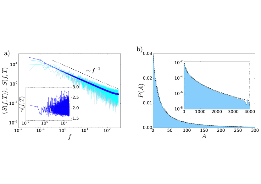
exist for any $n>0$ and, hence, all negative moments of $\int^{T}_{0}dtB_{t}^{2}$ exist, as well. As a consequence, $P(A)$ is an analytic function of $A$. We immediately obtain the coefficient of variation from (25) as $\gamma=\sqrt{17}/2$. Figure 11 displays numerical results for which we observe excellent agreement with the theoretical expressions.

7 Conclusions

Quite typically stochastic time series are evaluated in terms of the ensemble averaged MSD $\left\langle\overline{x_{t}^{2}}\right\rangle_{\Psi}$. It has the advantage that fluctuations are reduced due to the averaging over many individual trajectories. However, this is not always possible. Namely, for the by-now routine results from single particle tracking experiments typically rather few, finite time series are obtained. These are then evaluated in terms of the time-averaged MSD. While this quantity may also be averaged over the available individual trajectories, it is increasingly realised that the amplitude fluctuations between individual trajectories in fact harbours important quantitative information characteristic for a given stochastic process [14, 15, 116, 117, 118].

Similar to the consideration of time averaged MSDs for trajectories of finite measurement time $T$, we here analysed the single-trajectory PSD of stochastic trajectories characterised by random diffusivities. Following our previous work on standard Brownian motion [76], as well as fractional [77] and scaled Brownian motion [78], we here investigated the detailed behaviour of single-trajectory PSDs of a broad class of diffusing-diffusivity models. These have recently gained considerable attention as simple models for diffusion processes in heterogeneous media. We described a general procedure to obtain the position PDF ${\bf\Pi}(x,t)$ for all such models. The main ingredient in the calculation is the MGF of the integrated diffusivity, showing explicitly that different choices of the underlying diffusivity $\Psi_{t}$ lead to distinctly different emerging behaviours, as summarised in Table 1).

Random diffusivity model		MGF of $\tau_{T}$	${\bf\gamma}$	Ageing
$\Psi_{t}=Y_{t}^{2},\quad$ $Y_{t}=$ OU process		Eq. (30)	Eq. (31)	$\times$
$\Psi_{t}=\psi_{k}$	$\rho(\psi)$ gamma distr.	Eq. (38)	Eq. (47)	$\times$
	$\rho(\psi)$ Lévy-Smirnov distr.	Eq. (53)	not defined	not defined
$\Psi_{t}=V[B_{t}]$	$V[Z]=\theta(Z)$	Eq. (61)	$\sqrt{19/8}$	$\times$
	$V[Z]=\exp(-Z)$	Eq. (78)	Eq. (83)	$\checkmark$
	$V[Z]=Z^{2}$	Eq. (86)	$\sqrt{17}$/2	$\checkmark$

Table 1: Collection of the main results for the different random diffusivity models with respective equation numbers. Next to the definitions of the models we refer to the MGF of the integrated diffusivity $\tau_{T}$, the coefficient of variation $\gamma$, which can play the role of an indicator for each model, and the ageing behaviour.

We started our discussion from the by-now well-established and widely studied model of "diffusing-diffusivity", namely the case when $\Psi_{t}$ is chosen as the squared of the Ornstein-Uhlenbeck process. We then discussed the second case, in which $\Psi_{t}$ is defined as a jump process. The properties of this model depend strongly on the exact distribution chosen for the increment variables. We considered two examples, a Gamma distribution and a Lévy-Smirnov distribution. Finally, three cases in which the diffusivity is modelled as a functional of Brownian motion were discussed.

The main result of this work is that, regardless of the different properties of all these diffusing-diffusivity models we obtained a universal high-$f$ asymptote of the PSD. This behaviour is characterised by a $1/f^{2}$ scaling, in analogy to Brownian motion [76] and scaled Brownian motion [78]. A first way to discriminate among models lies in the study of the ageing behaviour of the PSD, as already discussed in [78]. Indeed, we showed that the dependence of the PSD on the trajectory length $T$ appears only for those random diffusivity models that are characterised by an anomalous scaling of the MSD. We also showed that differences from one model to another appear in higher order moments. In particular, we obtained exact expressions for the coefficient of variation in all cases, proving that the latter can be a good indicator of the specific model (see Table 1).

Finally, we established that the PDF of the random amplitude $A$ carries most of the meaningful information. Namely, the coefficient of variation may be directly calculated from its moments. Moreover, its MGF is tightly related to that of the integrated diffusivity, thus reflecting the particular properties of the process $\Psi_{t}$. As we showed before [76, 77], the distribution $P(A)$ can even be evaluated meaningfully from experimental data of fairly short trajectories. In its useful role in data analysis the single-trajectory PSD approach thus complements other methods such as the time-averaged MSD and its amplitude variation [14, 116, 119, 120, 121, 122, 123, 124, 125], ageing analyses [77, 116], or, in the context of non-Gaussian diffusion, the codifference methods [126].

The role of distinguishing different physical processes from measured single trajectory data therefore heavily lies on the amplitude fluctuations and the coefficient of variation encoded in them. This improved understanding of the single-trajectory PSD should therefore replace a common claim in many textbooks according to which the $1/f^{2}$-dependence of the spectrum was a fingerprint of Brownian motion. In line to previous works [76, 77, 78], in which we already alerted that this may be a deceptive concept, we have shown here that a wide range of random-diffusivity models with distinctly different behaviour and showing anomalous diffusion, exhibit precisely the $1/f^{2}$-dependence. Therefore, any experimental observation of the spectral density varying as $1/f^{2}$ alone cannot be taken as proof of standard Brownian motion. One necessarily needs to consider the ageing behaviour of the spectral density, as in the case of superdiffusive fractional Brownian motion or scaled Brownian motion, evaluate the coefficient of variation of the spectral density, or determine the functional form of the PDF $P(A)$ of the amplitude fluctuations.

In light of this the relevance of the presented results is twofold. First, they provide new and useful insights into the increasingly popular class of stochastic processes with random diffusivity used in the description of Fickian yet non-Gaussian diffusion in heterogeneous systems. Second, the results continue our ongoing analysis based on the single-trajectory PSD for different classes of stochastic processes, showing in particular the persistence of the $1/f^{2}$-scaling of the PSD, which appears to be robust—as long as we do not introduce correlations in the driving noise of the system, as studied in [77].

We note that if we redefine $\dot{x}_{t}$ in the Langevin equation (3) as $\dot{S}_{t}/S_{t}$, we recover the seminal Black-Scholes (or Black-Scholes-Merton) equation for an asset price $S_{t}$ with zero-constant trend and stochastic volatility $\sqrt{D_{0}\Psi_{t}}$ used in financial market models [127, 128, 129]. The relevance of diffusing-diffusivity approaches to economic and financial modelling was also discussed for the case of the squared Ornstein-Uhlenbeck process [61]. Namely, the resulting stochastic equation for $D_{0}\Psi_{t}$ in this case is nothing else than the Heston model [130], a special class of the Cox-Ingersson-Ross model [131, 132], and as such specifies the time evolution of the stochastic volatility of a given asset [63, 130, 133].

We finally note that realisation-to-realisation fluctuations of a stochastic process also turn out to be relevant in many scenarios of first-passage time statistics [134, 135]. These fluctuations are connected to the typically broad ("defocused") PDFs of first-passage times even in simple geometries [136, 137]. It will be interesting to extend the existing first-passage time analyses of diffusing-diffusivity models [64, 68] to the different processes studied herein, and to more complex geometries.

Appendix A Derivation of the moment-generating function of the power spectral density

It is convenient to rewrite formally the definition of the PSD in (8) in the form

$$S_{T}(f)=\frac{1}{T}\left(\int^{T}_{0}dt\cos(ft)x_{t}\right)^{2}+\frac{1}{T}\left(\int^{T}_{0}dt\sin(ft)x_{t}\right)^{2}.$$ (98)

Our first step then consists in a standard linearisation of the expression in the exponential in (9). Taking advantage of the integral identity

$$\exp\bigl{(}-b^{2}/(4c)\bigr{)}=\sqrt{\frac{c}{\pi}}\int^{\infty}_{-\infty}dz\exp(-cz^{2}+ibz)$$ (99)

for $c>0$, we formally recast (9) into the form

$$\qquad\phi_{\lambda}=\frac{1}{4\pi\lambda}\int^{\infty}_{-\infty}dz_{1}\int^{\infty}_{-\infty}dz_{2}\exp\left(-\frac{z_{1}^{2}+z_{2}^{2}}{4\lambda}\right)\left\langle\overline{\exp\left(i\int^{T}_{0}dtQ_{t}x_{t}\right)}\right\rangle_{\Psi},$$ (100)

where $Q_{t}$ is defined in (11). Now, the averaging over thermal noise realisations can be performed straightforwardly, yielding

$$\overline{\exp\left(i\int^{T}_{0}dtQ_{t}x_{t}\right)} = \overline{\exp\left(i\sqrt{2D_{0}}\int^{T}_{0}dt\sqrt{\Psi_{t}}\xi_{t}\int^{T}_{t}d\tau Q_{\tau}\right)}$$ (101)

$$= \exp\left(-D_{0}\int^{T}_{0}dt\Psi_{t}\left(\int^{T}_{t}d\tau Q_{\tau}\right)^{2}\right),$$

where we integrated by parts and used (3). Combining (101) and (100) we arrive at our general result (10).

The derivation of our main result (13) takes advantage of the explicit form of $Q$ in (11) and the following calculation,

$$\qquad\int^{T}_{0}dt\Psi_{t} \left(\int^{T}_{t}d\tau Q_{\tau}\right)^{2}=\frac{z_{1}^{2}}{f^{2}T}\int^{T}_{0}dt\Psi_{t}\bigg{(}\sin(fT)-\sin(ft)\bigg{)}^{2}$$ (102)

$$+\frac{z_{2}^{2}}{f^{2}T}\int^{T}_{0}dt\Psi_{t}\bigg{(}\cos(ft)-\cos(fT)\bigg{)}^{2}$$

$$+\frac{2z_{1}z_{2}}{f^{2}T}\int^{T}_{0}dt\Psi_{t}\bigg{(}\sin(fT)-\sin(ft)\bigg{)}\bigg{(}\cos(ft)-\cos(fT)\bigg{)}.$$

Inserting the latter expression into (10) and performing the integrations over $z_{1}$ and $z_{2}$ we find the expression in (13) with $L_{f}(t_{1},t_{2})$ explicitly defined by

$$L_{f} (t_{1},t_{2})=\frac{1}{2}\cos(2ft_{2})-\frac{1}{2}\cos(2ft_{1})-\frac{1}{2}\cos(f(T-t_{1}))-\frac{1}{2}\cos(f(T-t_{2}))$$ (103)

$$-\frac{1}{4}\cos(2f(T-t_{1}))-\frac{1}{2}\cos(2f(T-t_{2}))+\frac{1}{4}\cos(f(3T-t_{2}))$$

$$-\frac{1}{4}\cos(f(3T-t_{1}))+\frac{3}{4}\cos(f(T+t_{1}))-\frac{3}{4}\cos(f(T+t_{2}))-\frac{1}{2}\cos(f(t_{1}-t_{2}))$$

$$-\frac{1}{4}\cos(2f(t_{1}-t_{2}))+\frac{1}{4}\cos(f(T-2t_{1}-t_{2}))-\frac{1}{4}\cos(f(T-t_{1}-2t_{2}))$$

$$+\frac{1}{2}\cos(f(T+t_{1}-2t_{2}))+\frac{1}{2}\cos(f(T-2t_{1}+t_{2}))+\frac{1}{4}\cos(f(T+2t_{1}-t_{2}))$$

$$-\frac{1}{4}\cos(f(T-t_{1}+2t_{2}))+\frac{1}{2}\cos(f(2T-t_{1}-t_{2}))-\frac{1}{2}\cos(f(2T+t_{1}-t_{2}))$$

$$+\frac{1}{2}\cos(f(2T-t_{1}+t_{2})).$$

Appendix B High-$f$ behaviour of the Riemann-integrable diffusivities

For Riemann-integrable functions, according to the Riemann-Lebesgue lemma we have

$$\lim_{f\to\infty}\int^{T}_{0}dt\Psi_{t}\cos(f(T-t))=0$$ (104)

with probability $1$ (however, nothing can be said about how fast zero is approached in the general case). Once (104) holds, one finds that for $L_{f}(t_{1},t_{2})$ defined in (103),

$$\lim_{f\to\infty}\int^{T}_{0}dt_{1}\Psi_{t_{1}}\int^{T}_{0}dt_{2}\Psi_{t_{2}}L_{f}(t_{1},t_{2})=0.$$ (105)

Appendix C Useful formulae

Our expression for the PDF $P(A)$ in (26) and (27) rely on the following series expansion of the product of two Bessel functions,

$$J_{0} \left(\left(1+\frac{1}{\sqrt{3}}\right)\sqrt{2zA}\right)J_{0}\left(\left(1-\frac{1}{\sqrt{3}}\right)\sqrt{2zA}\right)$$ (106)

$$=\sum_{n=0}^{\infty}\frac{(-1)^{n}}{(n!)^{2}}\left(\frac{\sqrt{3}+1}{\sqrt{6}}\right)^{2n}\,_{2}F_{1}\left(-n,-n;1;\frac{1-\sqrt{3}/2}{1+\sqrt{3}/2}\right)(zA)^{n}.$$

The form of the PDF in (95) stems from the expansion

$$\qquad\frac{\displaystyle 1}{\displaystyle\sqrt{\cosh\left(\sqrt{4D_{B}Tz/a^{2}}\right)}}=\sqrt{2}\sum_{n=0}^{\infty}{{-1/2}\choose{n}}\exp\left(-2\sqrt{\frac{D_{B}Tz}{a^{2}}}\left(2n+\frac{1}{2}\right)\right).$$ (107)

The result in (69) involves toroidal functions defined by

$$\qquad P_{n-1/2}\left(\cosh(\eta)\right)=\frac{\displaystyle 2}{\displaystyle\pi}e^{-(n+1/2)\eta}\int^{\pi/2}_{0}\frac{\displaystyle d\phi}{\displaystyle\left(1-2e^{-\eta}\sinh(\eta)\sin^{2}(\phi)\right)^{n+1/2}}.$$ (108)

Setting $\exp(-\eta)\sinh(\eta)=1/3$, i.e., $\eta=\ln(\sqrt{3})$, we obtain expression (69).

References

- [1] R. Brown, A brief account of microscopical observations made in the months of June, July and August 1827, on the particles contained in the pollen of plants; and on the general existence of active molecules in organic and inorganic bodies, Phil. Mag. 4, 161 (1828).
- [2] A. Fick, Über Diffusion (On Diffusion), Ann. Phys. (Leipzig) 170, 59 (1855).
- [3] A. Einstein, Über die von der molekularkinetischen Theorie der Wärme geforderte Bewegung von in ruhenden Flüssigkeiten suspendierten Teilchen (On the motion of small particles suspended in liquids at rest required by the molecular-kinetic theory of heat), Ann. Phys. (Leipzig) 322, 549 (1905).
- [4] M. von Smoluchowski, Zur kinetischen Theorie der Brownschen Molekularbewegung und der Suspensionen (On the kinetic theory of Brownian molecular motion and suspensions), Ann. Phys. (Leipzig) 21, 756 (1906).
- [5] W. Sutherland, A dynamical theory of diffusion for non-electrolytes and the molecular mass of albumin, Philos. Mag. 9, 781 (1905).
- [6] K. Pearson, The Problem of the Random Walk, Nature 72, 294 (1905).
- [7] P. Langevin, On the theory of Brownian motion, C. R. Acad. Sci. Paris 146, 530 (1908).
- [8] F. Höfling and T. Franosch, Anomalous transport in the crowded world of biological cells, Rep. Progr. Phys. 76, 046602 (2013).
- [9] K. Nørregaard, R. Metzler, C. M. Ritter, K. Berg-Sørensen, and L. B. Oddershede, Manipulation and motion of organelles and single molecules in living cells, Chem. Rev. 117, 4342 (2017).
- [10] X. S. Xie, P. J. Choi, G.-W. Li, N. K. Lee, and G. Lia, Single-Molecule Approach to Molecular Biology in Living Bacterial Cells, Annu. Rev. Biophys. 37, 417 (2008).
- [11] C. Bräuchle, D. C. Lamb, and J. Michaelis, Single Particle Tracking and Single Molecule Energy Transfer (Wiley-VCH, Weinheim, Germany, 2012).
- [12] M. Javanainen H. Martinez-Seara, R. Metzler, and I. Vattulainen, Diffusion of Integral Membrane Proteins in Protein-Rich Membranes, J. Phys. Chem. Lett. 8, 4308 (2017).
- [13] X. Hu, L. Hong, M. D. Smith, T. Neusius, X. Cheng, and J. C. Smith, The dynamics of single protein molecules is non-equilibrium and self-similar over thirteen decades in time, Nature Phys. 12, 171 (2016).
- [14] E. Barkai, Y. Garini, and R. Metzler, Strange Kinetics of Single Molecules in Living Cells, Phys. Today 65(8), 29 (2012).
- [15] D. Krapf and R. Metzler, Strange interfacial molecular dynamics, Phys. Today 72(9), 48 (2019).
- [16] R. Metzler, Brownian motion and beyond: first-passage, power spectrum, non-Gaussianity, and anomalous diffusion, J. Stat. Mech. (2019) 114003.
- [17] J. Klafter, M. F. Shlesinger, and G. Zumofen, Beyond Brownian Motion, Phys. Today 49(6), 33 (1996).
- [18] M. Shlesinger, G. Zaslavsky, and J. Klafter, Strange kinetics, Nature 363, 31 (1993).
- [19] H. Scher, M. F. Shlesinger, and J. T. Bendler, Time-Scale Invariance in Transport and Relaxation, Phys. Today 44(1), 26 (1991).
- [20] M. J. Saxton and K. Jacobsen, Single-particle tracking: applications to membrane dynamics, Ann. Rev. Biophys. Biomol. Struct. 26, 373 (1997).
- [21] I. Golding and E. C. Cox, Physical Nature of Bacterial Cytoplasm, Phys. Rev. Lett. 96, 098102 (2006).
- [22] S. C. Weber, A. J. Spakowitz, and J. A. Theriot, Bacterial Chromosomal Loci Move Subdiffusively through a Viscoelastic Cytoplasm, Phys. Rev. Lett. 104, 238102 (2010).
- [23] K. Burnecki, E. Kepten, J. Janczura, I. Bronshtein, Y. Garini, and A. Weron, Universal Algorithm for Identification of Fractional Brownian Motion. A Case of Telomere Subdiffusion, Biophys. J. 103, 1839 (2012).
- [24] I. Bronstein, Y. Israel, and Y. Garini, Transient anomalous diffusion of telomeres in the nucleus of mammalian cells, Phys. Rev. Lett. 103, 018102 (2009).
- [25] J.-H. Jeon, V. Tejedor, S. Burov, E. Barkai, C. Selhuber-Unkel, K. Berg-Sørensen, L. Oddershede, and R. Metzler, In vivo anomalous diffusion and weak ergodicity breaking of lipid granules, Phys. Rev. Lett. 106, 048103 (2011).
- [26] E. Bertseva, D. S. Grebenkov, P. Schmidhauser, S. Gribkova, S. Jeney, and L. Forro, Optical Trapping Microrheology in Cultured Human Cells, Eur. Phys. J. E 35, 63 (2012).
- [27] A. V. Weigel, B. Simon, M. M. Tamkun, and D. Krapf, Ergodic and nonergodic processes coexist in the plasma membrane as observed by single-molecule tracking, Proc. Natl. Acad. Sci. USA 108, 6438 (2011).
- [28] C. Manzo, J. A. Torreno-Pina, P. Massignan, G. J. Lapeyre, Jr., M. Lewenstein, and M. F. Garcia Parajo, Weak ergodicity breaking of receptor motion in living cells stemming from random diffusivity, Phys. Rev. X 5, 011021 (2015).
- [29] J. Szymanski and M. Weiss, Elucidating the origin of anomalous diffusion in crowded fluids, Phys. Rev. Lett. 103, 038102 (2009).
- [30] J.-H. Jeon, N. Leijnse, L. B. Oddershede, and R. Metzler, Anomalous diffusion and power-law relaxation in wormlike micellar solution, New J. Phys. 15, 045011 (2013).
- [31] C. Di Rienzo, V. Piazza, E. Gratton, F. Beltram, and F. Cardarelli, Probing short-range protein Brownian motion in the cytoplasm of living cells, Nature Comm. 5, 5891 (2014).
- [32] K. Chen, B. Wang, and S. Granick, Memoryless self-reinforcing directionality in endosomal active transport within living cells, Nature Mat. 14, 589 (2015).
- [33] D. Robert, T. H. Nguyen, F. Gallet, and C. Wilhelm, In vivo determination of fluctuating forces during endosome trafficking using a combination of active and passive microrheology, PLoS ONE 4, e10046 (2010).
- [34] A. Caspi, R. Granek, and M. Elbaum, Enhanced diffusion in active intracellular transport, Phys. Rev. Lett. 85, 5655 (2000).
- [35] M. S. Song, H. C. Moon, J.-H. Jeon, and H. Y. Park, Neuronal messenger ribonucleoprotein transport follows an aging Lévy walk, Nat. Comm. 9, 344 (2018).
- [36] J. F. Reverey, J.-H. Jeon, H. Bao, M. Leippe, R. Metzler, and C. Selhuber-Unkel, Superdiffusion dominates intracellular particle motion in the supercrowded space of pathogenic Acanthamoeba castellanii, Sci. Rep. 5, 11690 (2015).
- [37] B. Wang, J. Kuo, S. C. Bae, and S. Granick, When Brownian diffusion is not Gaussian, Nat. Mater. 11, 481 (2012).
- [38] B. Wang, S. M. Anthony, S. C. Bae, and S. Granick, Anomalous yet Brownian, Proc. Natl. Acad. Sci. USA 106, 15160 (2009).
- [39] J. Guan, B. Wang, and S. Granick, Single-molecule observation of long jumps in polymer adsorption, ACS Nano 8, 3331 (2014).
- [40] K. He, F. B. Khorasani, S. T. Retterer, D. K. Tjomasn, J. C. Conrad, and R. Krishnamoorti, Diffusive dynamics of nanoparticles in arrays of nanoposts, ACS Nano 7, 5122 (2013).
- [41] C. Xue, X. Zheng, K. Chen, Y. Tian, and G. Hu, Probing non-Gaussianity in confined diffusion of nanoparticles, J. Phys. Chem. Lett. 7, 514 (2016).
- [42] D. Wang, R. Hu, M. J. Skaug, and D. Schwartz, Temporally anticorrelated motion of nanoparticles at a liquid interface, J. Phys. Chem. Lett. 6 54 (2015).
- [43] S. Dutta and J. Chakrabarti, Anomalous dynamical responses in a driven system, EPL 116, 38001 (2016).
- [44] K. C. Leptos, J. S. Guasto, J. P. Gollub, A. I. Pesci, and R. E. Goldstein, Dynamics of enhanced tracer diffusion in suspensions of swimming eukaryotic microorganisms, Phys. Rev. Lett. 103, 198103 (2009).
- [45] S. Hapca, J. W. Crawford, and I. M. Young, Anomalous diffusion of heterogeneous populations characterized by normal diffusion at the individual level, J. R. Soc. Interface 6, 111 (2009).
- [46] P. Witzel, M. Götz, Y. Lanoiselée, T. Franosch, D. S. Grebenkov, and D. Heinrich, Heterogeneities Shape Passive Intracellular Transport, Biophys. J. 117, 203 (2019).
- [47] A. G. Cherstvy, O. Nagel, C. Beta, and R. Metzler, Non-Gaussianity, population heterogeneity, and transient superdiffusion in the spreading dynamics of amoeboid cells, Phys. Chem. Chem. Phys., 20, 23034 (2018).
- [48] J.-H. Jeon, M. Javanainen, H. Martinez-Seara, R. Metzler, and I. Vattulainen, Protein crowding in lipid bilayers gives rise to non-Gaussian anomalous lateral diffusion of phospholipids and proteins, Phys. Rev. X 6, 021006 (2016).
- [49] C. Beck and E. G. D. Cohen, Superstatistics, Physica A 332, 267 (2003).
- [50] C. Beck, Statistics of three-dimensional Lagrangian turbulence, Phys. Rev. Lett. 98, 064502 (2007).
- [51] C. Beck, Stretched exponentials from superstatistics, Physica A 365, 96 (2006).
- [52] E. van der Straeten and C. Beck, Superstatistical fluctuations in time series: Applications to share-price dynamics and turbulence, Phys. Rev. E 80, 036108 (2009).
- [53] R. Metzler, Superstatistics and non-Gaussian diffusion, Euro. Phys. J. Special Topics (at press).
- [54] F. Baldovin, E. Orlandini, and F. Seno, Polymerization induces non-Gaussian diffusion, Frontiers Phys. 7, 124 (2019) .
- [55] A. Mura, M. S. Taqqu, and F. Mainardi, Non-Markovian diffusion equations and processes: analysis and simulations, Physica A 387, 5033 (2008).
- [56] A. Mura and G. Pagnini, Characterizations and simulations of a class of stochastic processes to model anomalous diffusion, J. Phys. A 41, 285003 (2008).
- [57] D. Molina-García, T. Minh Pham, P. Paradisi, C. Manzo, and G. Pagnini, Fractional kinetics emerging from ergodicity breaking in random media, Phys. Rev. E 94, 052147 (2016).
- [58] Chubynsky MV and Slater GW, Diffusing Diffusivity: A Model for Anomalous, yet Brownian, Diffusion, Phys. Rev. Lett. 113, 098302 (2014).
- [59] R. Jain and K. L. Sebastian, Diffusion in a Crowded, Rearranging Environment, J. Phys. Chem. B 120, 3988 (2016).
- [60] R. Jain and K. L. Sebastian, Diffusing diffusivity: survival in a crowded rearranging and bounded domain, J. Phys. Chem. B 120, 9215 (2016).
- [61] A. V. Chechkin, F. Seno, R. Metzler, and I. M. Sokolov, Brownian Yet Non-Gaussian Diffusion: From Superstatistics to Subordination of Diffusing Diffusivities, Phys. Rev. X 7, 021002 (2017).
- [62] N. Tyagi and B. J. Cherayil, Non-Gaussian Brownian diffusion in dynamically disordered thermal environments, J. Phys. Chem. B 121, 7204 (2017).
- [63] Y. Lanoiselée and D. S. Grebenkov, A model of non-Gaussian diffusion in heterogeneous media, J. Phys. A. 51, 145602 (2018).
- [64] Y. Lanoiselée, N. Moutal, and D. S. Grebenkov, Diffusion-limited reactions in dynamic heterogeneous media, Nature Commun. 9, 4398 (2018).
- [65] V. Sposini, A. V. Chechkin, F. Seno, G. Pagnini, and R. Metzler, Random diffusivity from stochastic equations: comparison of two models for Brownian yet non-Gaussian diffusion, New. J. Phys. 20, 043044 (2018).
- [66] D. S. Grebenkov, A unifying approach to first-passage time distributions in diffusing diffusivity and switching diffusion models, J. Phys. A 52, 174001 (2019).
- [67] Y. Lanoiselée and D. S. Grebenkov, Non-Gaussian diffusion of mixed origins, J. Phys. A 52, 304001 (2019).
- [68] V. Sposini, A. V. Chechkin, and R. Metzler, First passage statistics for diffusing diffusivity, J. Phys. A 52, 04LT01 (2019).
- [69] M. Hidalgo-Soria and E. Barkai, The Hitchhiker model for Laplace diffusion processes in the cell environment, E-print arXiv:1909.07189.
- [70] I. Chakraborty and Y. Roichman, Two coupled mechanisms produce Fickian, yet non-Gaussian diffusion in heterogeneous media E-print arXiv:1909.11364 (2019).
- [71] N. Shephard, Stochastic volatility models. In: S. N. Durlauf, L.E. Blume (eds) Macroeconometrics and Time Series Analysis. The New Palgrave Economics Collection. Palgrave Macmillan, London (2010).
- [72] O. Barndorff-Nielsen and N. Shephard, Non-Gaussian OU based models and some of their uses in financial economics, J. R. Stat. Soc. B 63, 167–241 (2001).
- [73] S. Sadegh, E. Barkai and D. Krapf, 1/f noise for intermittent quantum dots exhibits non-stationarity and critical exponents, New J. Phys. 16, 113054 (2014).
- [74] N. Leibovich,A. Dechant, E. Lutz, and E. Barkai, Aging Wiener-Khinchin Theorem and Critical Exponents of Noise, Phys. Rev. E 94, 052130 (2016).
- [75] N. Leibovich and E. Barkai, Conditional noise: From single molecules to macroscopic measurement, Phys. Rev. E 96, 032132 (2017).
- [76] D. Krapf, E. Marinari, R. Metzler, G. Oshanin, X. Xu and A. Squarcini, Power spectral density of a single Brownian trajectory: what one can and cannot learn from it, New J. Phys. 20, 023029 (2018).
- [77] D. Krapf, N. Lukat, E. Marinari, R. Metzler, G. Oshanin, C. Selhuber-Unkel, A. Squarcini, L. Stadler, M. Weiss, and X. Xu, Spectral Content of a Single Non-Brownian Trajectory, Phys. Rev. X 9, 011019 (2019).
- [78] V. Sposini, R. Metzler and G. Oshanin, Single-trajectory spectral analysis of scaled Brownian motion, New J. Phys. 21, 073043 (2019).
- [79] S. C. Lim and S. V. Muniandy, Self-similar Gaussian processes for modeling anomalous diffusion, Phys. Rev. E 66, 021114 (2002).
- [80] J.-H. Jeon, A. V. Chechkin, and R. Metzler, Scaled Brownian motion: a paradoxical process with a time dependent diffusivity for the description of anomalous diffusion, Phys. Chem. Chem. Phys. 16, 15811 (2014).
- [81] J. Ślȩzak, K. Burnecki, and R. Metzler, Random coefficient autoregressive processes describe Brownian yet non-Gaussian diffusion in heterogeneous systems, New J. Phys. 21, 073056 (2019).
- [82] W. Feller, Two singular diffusion problems, Ann. Math. 54, 173 (1951).
- [83] J. C. Cox, J. E. Ingersoll, and S. A. Ross, A theory of the term structure of interest rates, Econometrica 53, 385 (1985).
- [84] S.L. Heston, A Closed-Form Solution for Options with Stochastic Volatility with Applications to Bond and Currency Options, Rev. Financial Studies 6, 327 (1993).
- [85] T. Dankel, On the distribution of the integrated square of the Ornstein-Uhlenbeck process, SIAM J. Appl. Math. 5, 568 (1991).
- [86] V. Tejedor and R. Metzler, Anomalous diffusion in correlated continuous time random walks, J. Phys. A 43, 082002 (2010).
- [87] M. Magdziarz, R. Metzler, W. Szczotka, and P. Zebrowski, Correlated continuous-time random walks – scaling limits and Langevin picture, J. Stat. Mech. P04010 (2012).
- [88] P. Lévy, Sur certains processus stochastiques homogènes (On certain homogeneous stochastic processes), Compositio Mathematica 7, 283 (1940).
- [89] R. H. Cameron and W. T. Martin, Transformations of Wiener integrals under a general class of linear transformation, Trans. Amer. Math. Soc. 58, 184 (1945);
- [90] R. H. Cameron and W. T. Martin, Evaluation of various Wiener integrals by use of certain Sturm-Liouville differential equations, Bull. Amer. Math. Soc. 51, 73 (1945).
- [91] M. Kac, On distributions of certain Wiener functionals, Trans. Amer. Math. Soc. 65, 1 (1949).
- [92] P. Erdös and M. Kac, On the number of positive sums of independent random variables, Bull. Amer. Math. Soc. 53, 1011 (1947).
- [93] J. Lamperti, An occupation time theorem for a class of stochastic processes, Trans. Amer. Math. Soc. 88, 380 (1958).
- [94] M. Yor, Exponential functionals of Brownian motion and related processes (Springer, Berlin, 2000).
- [95] S. N. Majumdar, Brownian functionals in physics and computer science, Current Science 89, 2076 (2005).
- [96] A. Perret, A. Comtet, S. N. Majumdar, and G. Schehr, On Certain Functionals of the Maximum of Brownian Motion and Their Applications, J. Stat. Phys. 161, 1112 (2015).
- [97] D. Boyer, D. S. Dean, C. Mejía-Monasterio, and G. Oshanin, Distribution of the least-squares estimators of a single Brownian trajectory diffusion coefficient, J. Stat. Mech. (2013) P04017.
- [98] D. Boyer, D. S. Dean, C. Mejía-Monasterio, and G. Oshanin, Optimal estimates of the diffusion coefficient of a single Brownian trajectory, Phys. Rev. E 85, 031136 (2012).
- [99] A. N. Borodin and P. Salminen, Handbook of Brownian Motion: Facts and Formulae, (Birkhäuser Verlag, Basel, 1996).
- [100] Arkhincheev V E and Baskin E M 1991 Anomalous diffusion and drift in a comb model of percolation clusters Sov. Phys. JETP 73, 161.
- [101] Sandev T, Iomin A, Kantz H, Metzler R and Chechkin A 2016 Comb model with slow and Ultraslow diffusion Math. Model. Nat. Phenom. 11, 18.
- [102] P. Lévy, Sur certains processus stochastiques homogènes, Compositio Mathematica 7, 283 (1939).
- [103] H. Geman and M. Yor, Bessel processes, Asian options, and perpetuities, Math. Finance 3, 349 (1993).
- [104] P. Wilmott, J. Dewynne, and S. Howison, Option Pricing: Mathematical Models and Computation, (Oxford Financial Press, 2000).
- [105] G. Oshanin and G. Schehr, Two stock options at the races: Black-Scholes forecasts, Quant. Finance 12, 1325 (2012).
- [106] O. Peters and W. Klein, Ergodicity breaking in geometric Brownian motion, Phys. Rev. Lett. 110, 100603 (2013).
- [107] A. G. Cherstvy, D. Vinod, E. Aghion, A. V. Chechkin, and R. Metzler, Time averaging, ageing and delay analysis of financial time series, New J. Phys. 19, 063045 (2017).
- [108] S. F. Burlatsky, G. Oshanin, A. Mogutov, and M. Moreau, Non-Fickian steady flux in a one-dimensional Sinai-type disordered system, Phys. Rev. A 45, R6955 (1992).
- [109] G. Oshanin, A. Mogutov and M. Moreau, Steady flux in a continuous-space Sinai chain, J. Stat. Phys. 73, 379 (1993).
- [110] C. Monthus and A. Comtet, On the flux distribution in a one dimensional disordered system, J. Phys. I. France 4, 635 (1994).
- [111] A. Comtet, C. Monthus, and M. Yor, Exponential functionals of Brownian motion and disordered systems, J. Appl. Probab. 35, 255 (1998).
- [112] G. Oshanin, A. Rosso, and G. Schehr, Anomalous fluctuations of currents in Sinai-type random chains with strongly correlated disorder, Phys. Rev. Lett. 110, 100602 (2013).
- [113] A. G. Cherstvy, A. V. Chechkin, and R. Metzler, Anomalous diffusion and ergodicity breaking in heterogeneous diffusion processes, New J. Phys. 15, 083039 (2013).
- [114] A. G. Cherstvy and R. Metzler, Non-ergodicity, fluctuations, and criticality in heterogeneous diffusion processes, Phys. Rev. E 90, 012134 (2014).
- [115] G. Oshanin and S. Redner, Helix or coil? Fate of a melting heteropolymer, Europhys. Lett. 85, 10008 (2009).
- [116] R. Metzler, J.-H. Jeon, A. G. Cherstvy, and E. Barkai, Anomalous diffusion models and their properties: non-stationarity, non-ergodicity, and ageing at the centenary of single particle tracking, Phys. Chem. Chem. Phys. 16, 24128 (2014).
- [117] F. D. Stefani, J. P. Hoogenboom, and E. Barkai, Beyond quantum jumps: Blinking nanoscale light emitters, Phys. Today 62(2), 34 (2009).
- [118] Y. Lanoiselée and D. S. Grebenkov, Revealing nonergodic dynamics in living cells from a single particle trajectory, Phys. Rev. E 93, 052146 (2016).
- [119] A. Weron, J. Janczura, E. Boryczka, T. Sungkaworn, and D. Calebiro, Statistical testing approach for fractional anomalous diffusion classification, Phys. Rev. E 99, 042149 (2019).
- [120] S. Bo, F. Schmidt, R. Eichhorn, and G. Volpe, Measurement of anomalous diffusion using recurrent neural networks, Phys. Rev. E 100, 010102 (2019).
- [121] S. Thapa, M. A. Lomholt, J. Krog, A. G. Cherstvy, and R. Metzler, Bayesian nested sampling analysis of single particle tracking data: maximum likelihood model selection applied to stochastic diffusivity data, Phys. Chem. Chem. Phys. 20, 29018 (2018).
- [122] A. G. Cherstvy, S. Thapa, C. E. Wagner, and R. Metzler, Non-Gaussian, non-ergodic, and non-Fickian diffusion of tracers in mucin hydrogels, Soft Matter 15, 2526 (2019).
- [123] J.-H. Jeon and R. Metzler, Analysis of short subdiffusive time series: scatter of the time averaged mean squared displacement, J. Phys. A 43, 252001 (2010).
- [124] D. S. Grebenkov, Probability Distribution of the Time-Averaged Mean-Square Displacement of a Gaussian Process, Phys. Rev. E 84, 031124 (2011).
- [125] A. Andreanov and D. S. Grebenkov, Time-averaged MSD of Brownian motion, J. Stat. Mech. (2012), P07001.
- [126] J. Ślȩzak, R. Metzler, and M. Magdziarz, Codifference can detect ergodicity breaking and non-Gaussianity, New J. Phys. 21, 053008 (2019).
- [127] F. Black and M. Scholes, The pricing of options and corporate liabilities, J. Polit. Econ. 81, 637 (1973).
- [128] R. C. Merton, Optimum consumption and portfolio rules in a continuous-time model, J. Econ. Theory 3, 373 (1971).
- [129] R. C. Merton, Option pricing when underlying stock returns are discontinuous, J. Financ. Econ. 3, 125 (1976).
- [130] S. L. Heston, A Closed-Form Solution for Options with Stochastic Volatility with Applications to Bond and Currency Options, Rev. Financial Studies 6, 327 (1993).
- [131] J. C. Cox and S. A. Ross, The valuation of options for alternative stochastic processes, J. Finan. Econom. 3, 145 (1976).
- [132] J. C. Cox, J. E. Ingersoll, and S. A. Ross, A Theory of the term structure of interest rates, Econometrica 53, 385 (1985).
- [133] A. A. Dragulescu and V. M. Yakovenko, Probability distribution of returns in the Heston model with stochastic volatility, Quant. Finance 2, 443 (2002).
- [134] C. Mejía-Monasterio, G. Oshanin, and G. Schehr, First passages for a search by a swarm of independent random searchers, J. Stat. Mech. P06022 (2011).
- [135] T. Mattos, C. Mejía-Monasterio, R. Metzler, and G. Oshanin, First passages in bounded domains: When is the mean first passage time meaningful?, Phys. Rev. E 86, 031143 (2012).
- [136] A. Godec and R. Metzler, Universal proximity effect in target search kinetics in the few encounter limit, Phys. Rev. X 6, 041037 (2016).
- [137] D. Grebenkov, R. Metzler, and G. Oshanin, Strong defocusing of molecular reaction times: geometry and reaction control, Comm. Chem. 1, 96 (2018).