A continuation method in Bayesian inference

Ben Mansour Dia College of Petroleum Engineering and Geosciences (CPG), King Fahd University of Petroleum and Minerals (KFUPM), Dhahran 31261, Saudi Arabia, ben.dia@kfupm.edu.sa
Abstract

We present a continuation method that entails generating a sequence of transition probability density functions from the prior to the posterior in the context of Bayesian inference for parameter estimation problems. The characterization of transition distributions, by tempering the likelihood function, results in a homogeneous nonlinear partial integro-differential equation whose existence and uniqueness of solutions are addressed. The posterior probability distribution comes as the interpretation of the final state of the path of transition distributions. A computationally stable scaling domain for the likelihood is explored for the approximation of the expected deviance, where we manage to hold back all the evaluations of the forward predictive model at the prior stage. It follows the computational tractability of the posterior distribution and opens access to the posterior distribution for direct samplings. To get a solution formulation of the expected deviance, we derive a partial differential equation governing the moments generating function of the log-likelihood. We show also that a spectral formulation of the expected deviance can be obtained for low-dimensional problems under certain conditions. The computational efficiency of the proposed method is demonstrated through three differents numerical examples that focus on analyzing the computational bias generated by the method, assessing the continuation method in the Bayesian inference with non-Gaussian noise, and evaluating its ability to invert a multimodal parameter of interest.

Keywords: Bayes’ theorem, Posterior distribution, Barbashin equation, Banach space, Moments generating function, Differential equations.

AMS 2010 subject classification: 62F15, 45E05, 35B60, 35F31, 65C05

1 Introduction

There is a broad consensus that in statistical problems for parameter estimation under uncertainty, the Bayesian approach provides the method of choice since it measures the uncertainty in the knowledge of the parameter of interest with the interpretation of the probability density function (PDF). The Bayesian approach to inverse problems leads to the theory of updating a prior PDF with the information carried by the data, see [7, 34], through the Bayes’ rule, with the aim of computing the expected value of a quantity of interest from the posterior PDF. One important challenge encountered, when deploying the Bayes’ theorem, is the non-accessibility of the posterior PDF, which stems from the fact that the normalizing factor, also known as the Bayes factor, is unknown. While significant strides have been made in designing sampling approaches that have access to the posterior PDF, the overwhelming majority of pertinent methods are either computationally demanding in terms of the number of evaluations of the forward predictive model or intractable. The computational tractability refers here to the ability of counting, a priori, the number of evaluations of the forward predictive model when approximating the posterior distribution.

The most common way of approximating the Bayes factor is to refer to it as the marginal distribution of the likelihood function. That approach is computationally expensive when it comes to estimate statistics under the posterior PDF. That intensive computational cost is somehow due to the large standard deviation of the prior PDF, rises the curse of dimensionality for deterministic integration methods, and likely suffers from numerical underflow for a vague prior knowledge. To overcome this issue, the importance sampling has been utilized in sophisticated settings: with Laplace approximation for estimating the expected information gain [5, 6], based on a multilayered construction to quantify the nuisance effect of some components of the parameter of interest on the expected information gain [10], and in an iterative form suitable to being employed in parallel computer architectures [24].

Alternatively, advance classes of Markov chain Monte Carlo (MCMC) have been constructed to address the computation of statistics under the posterior PDF, with the basic idea of overpassing the normalizing constant approximation. Therein, the intensive computational load remains a major issue. Moreover, the acceptance criterion in MCMC methods deters the ability to count the number of evaluations of the forward model and therefore produces the intractability of the posterior PDF. A careful and comprehensive analysis based on the non-Markovian aspect of the counting index process is presented in [36]. A methodological approach of inspecting the transition probabilities between the prior and the posterior distributions, commonly referred to as continuation methods, has been addressed to promote MCMC methods [16, 19].

We present a continuation method to address two challenging issues in Bayesian inverse problems, that of overcoming the computational intractability of the posterior distribution, and scanning the transition distributions between the prior and the posterior. We consider the continuous update of the distribution alongside to the optimal transport approach addressed in a series of papers [23, 25, 29]. The continuation method introduced in [29], and used in [16], formulates the inversion as optimal control of information transport from the prior to posterior where the PDF is interpreted by the solution of a Liouville type equation with the assumption of available partial observations.

Our approach is also an alternative that bypasses the normalizing factor estimation via marginal likelihood, and allows direct sampling from the posterior distribution in particular, and from any transition distribution between the prior and the posterior stages in general. As in [16], we characterize the transition PDF when connecting the prior to the posterior by tempering the likelihood so that a continuous analysis of the transition PDF can be performed to assess the information carried by the data. Thereupon, we address also the computational tractability aspect with a continuous and differentiable path sampling to model the update of the prior distribution up to the posterior stage with the only assumption of continuity of the forward model with respect to the parameter of interest.

The starting point consists of composing the likelihood function with a normalized power function, and then we derive the associated transition distribution, named power posterior distribution, using the associated Bayes’ theorem. The characterization of the power posterior distribution results in a partial integro-differential equation (PIDE) whose solution at the final state is the posterior PDF. The existence and uniqueness of the solution of the characteristic equation follow from the analysis of boundary value problems of PIDE of Barbashin type presented in [1, 2, 3, 4, 18].

The computational tractability of the posterior PDF is reduced to the computational tractability of the expected deviance which, in turn, is obtained in two different ways. The first one assumes a null skewness condition and is derived from the spectral expansion of the kernel associated with the log-likelihood. The second formulation is built through the solution of a partial differential equation governing the moments generating function of the log-likelihood function.

We assess the effectiveness of our method with three numerical examples. The first example is a one-dimensional algebraic forward model with additive Gaussian noise, where analytical computations facilitate an error analysis. The second example is a source inversion problem, where the forward model is the solution of the one-dimensional wave equation. In that problem, we test our method to a complicated setting of the measurement errors formed by the combination of speckle noise and uniform noise. The Wasserstein distance is used to incorporate the noise in the likelihood definition. The objective is to infer the source location and the constant amplitude of waves propagating in a one-dimensional direction. The third example is a multimodal inversion that constitutes a challenging benchmark test for sampling methods.

Our contributions are presented as follows. The power posterior notion and its characterization are presented in Section 2. In Section 3, we detail the mathematical analysis to address the existence and the uniqueness of the characteristic PIDE equation. Explicit solution formulations for tractable transition distributions are established in Section 4. Section 5 is dedicated to numerical experiments performed to evaluate our continuation method.

2 Power-posterior formulation

In this section, we start by stating the Bayesian inversion problem and introduce the continuation method by tempering the likelihood. The characterization of the transition distribution is also presented.

2.1 Bayesian inversion

Let d𝑑d be a non-negative integer, 𝜽tdsubscript𝜽𝑡superscript𝑑\bm{\theta}_{t}\in\mathbb{R}^{d} be the true vector value of an unknown parameter that operates as an input in a forward predictive model denoted by 𝒈𝒈\bm{g}. We address the inference of the model parameter 𝜽tsubscript𝜽𝑡\bm{\theta}_{t}, given the forward model 𝒈𝒈\bm{g} and noisy dataset 𝒀q𝒀superscript𝑞\bm{Y}\in\mathbb{R}^{q} formed of q𝑞q observed quantities of the forward model output 𝒈(𝜽t)𝒈subscript𝜽𝑡\bm{g}(\bm{\theta}_{t}) polluted with measurement noise. We consider computationally intensive Bayesian inverse problems, where almost the entire computational load is associated with the evaluation of 𝒈𝒈\bm{g}.

From now, the parameter of interest is assumed to be a random variable vector, denoted by 𝜽𝜽\bm{\theta} in lieu of 𝜽tsubscript𝜽𝑡\bm{\theta}_{t}, and is characterized by a prior PDF π(𝜽)𝜋𝜽\pi(\bm{\theta}) with 𝜽=(θ1(ω1),,θd(ωd))T𝜽superscriptsubscript𝜃1subscript𝜔1subscript𝜃𝑑subscript𝜔𝑑𝑇\bm{\theta}=(\theta_{1}(\omega_{1}),\cdots,\theta_{d}(\omega_{d}))^{T}, ωiΩsubscript𝜔𝑖Ω\omega_{i}\in\Omega, where ΩΩ\Omega is the set of all random events. The density π(𝜽)𝜋𝜽\pi(\bm{\theta}) is a prior PDF on 𝜽tsubscript𝜽𝑡\bm{\theta}_{t} that is available to us, and the inference consists in updating that knowlegde on the parameter to the posterior density π(𝜽|𝒀)𝜋conditional𝜽𝒀\pi(\bm{\theta}|\bm{Y}) through the data 𝒀𝒀\bm{Y} with distribution p(𝒀)𝑝𝒀p(\bm{Y}). For that, we consider the Bayes’ theorem given by

π(𝜽|𝒀)=p(𝒀|𝜽)π(𝜽)p(𝒀),𝜋conditional𝜽𝒀𝑝conditional𝒀𝜽𝜋𝜽𝑝𝒀\displaystyle\pi(\bm{\theta}|\bm{Y})=\frac{p(\bm{Y}|\bm{\theta})\pi(\bm{\theta})}{p(\bm{Y})}, (1)

where p(𝒀|𝜽)𝑝conditional𝒀𝜽p(\bm{Y}|\bm{\theta}) is the likelihood, i.e. the function that measures how the dataset 𝒀𝒀\bm{Y} is distributed for each possible value 𝜽𝜽\bm{\theta} of the parameter. The selection of the likelihood is crucial in the Bayesian approach, is associated with the type of the measurement errors, and leads to the model specification. Efficient Bayesian inference, in terms of assessing the measurement errors and covering as well the model misspecification, appeals to designing the likelihood function through an optimal mapping problem for the transport of the information [14, 37]. In this work, we focus on a general exponential-type likelihood function covering complicated noise structures, and given by

p(𝒀|𝜽)=Cexp(s𝐝𝐢𝐬(𝒀,𝒈(𝜽))).𝑝conditional𝒀𝜽C𝑠𝐝𝐢𝐬𝒀𝒈𝜽\displaystyle p(\bm{Y}|\bm{\theta})=\text{C}\exp\left(-s\operatorname{\bf dis}(\bm{Y},\bm{g}(\bm{\theta}))\right). (2)

Here s𝑠s is a parameter that quantifies the dispersion of the measurement error on the data, C is a constant depending on d𝑑d and s𝑠s, i.e CC(d,s)CC𝑑𝑠\text{C}\equiv\text{C}(d,s), and 𝐝𝐢𝐬𝐝𝐢𝐬\operatorname{\bf dis} denotes a given quadratic distance between the data sample and the forward model output sample. Possible choices for the distance 𝐝𝐢𝐬𝐝𝐢𝐬\operatorname{\bf dis} are the Wasserstein distance, the Hellinger distance, the total variation distance, the Mahalanobis distance. Weighted versions of the mentioned distances by the distribution of the data noise are also admissible.

2.2 Power Bayes’ rule: a continuation method

We aim to derive a continuation method that consists of producing a sequence of transition distributions, named power posterior distributions, between the prior and the posterior stages, and that is computationally tractable. The concept of power posterior, used throughout this paper, is derived from the power Bayes’ rule, and based on the thermodynamic integration that is a widely used for computing the Bayes factor in physical applications, see [12, 13, 20]. It is a kind of a geometric path sampling known as parallel tempering method see [15, 8] or replica-exchange method in molecular dynamics see [35, 22], which are devised to advance MCMC methods.

The power Bayes’ rule is a readjusted Bayes’ rule in the framework of the continuation of distribution from the prior to the posterior. For a given real α[0,1]𝛼01\alpha\in[0,1], the power posterior distribution is given by

π(𝜽|𝒀;α)=p(𝒀|𝜽)απ(𝜽)z(𝒀|α),𝜋conditional𝜽𝒀𝛼𝑝superscriptconditional𝒀𝜽𝛼𝜋𝜽𝑧conditional𝒀𝛼\displaystyle\pi(\bm{\theta}|\bm{Y};\alpha)=\frac{p(\bm{Y}|\bm{\theta})^{\alpha}\pi(\bm{\theta})}{z(\bm{Y}|\alpha)}, (3)

where z(𝒀|α)𝑧conditional𝒀𝛼z(\bm{Y}|\alpha) is the normalizing constant and can be expressed as the marginal power likelihood. The variable α𝛼\alpha is the inverse tempering temperature, which is named here tempering parameter for easy convenience. For the tempering parameter α𝛼\alpha varying from 00 to 111, the power posterior PDF encodes the knowledge about the parameter of interest from the prior π(𝜽)=π(𝜽|𝒀;α)|α=0\pi(\bm{\theta})=\pi(\bm{\theta}|\bm{Y};\alpha)_{|\alpha=0} to the posterior π(𝜽|𝒀)=π(𝜽|𝒀;α)|α=1\pi(\bm{\theta}|\bm{Y})=\pi(\bm{\theta}|\bm{Y};\alpha)_{|\alpha=1}, and the normalizing factor z(𝒀|α)𝑧conditional𝒀𝛼z(\bm{Y}|\alpha) carries the data information of the ”full evidence” 1=z(𝒀|α)|α=01=z(\bm{Y}|\alpha)_{|\alpha=0} to the sample evidence p(𝒀)=z(𝒀|α)|α=1p(\bm{Y})=z(\bm{Y}|\alpha)_{|\alpha=1}.

The notation 𝔼𝔼\mathbb{E} stands for the expectation operator (with respect to the prior PDF), a subscript will be used to specify the associated random variable whenever there is a need for extra clarity. The Leibniz integral rule and the property of interchanging the integral over ΘΘ\Theta, the space of the parameter of interest, and the derivation with respect to the tempering parameter α𝛼\alpha are widely used throughout the manuscript. We will comment on it whenever the utilization seems not obvious.

Next, we characterize the power posterior PDF π(𝜽|𝒀;α)𝜋conditional𝜽𝒀𝛼\pi(\bm{\theta}|\bm{Y};\alpha) with a dynamical equation of which the solution at the final state α=1𝛼1\alpha=1 stands for the posterior PDF.

2.3 Characterization of the power posterior PDF

We present the derivation of the equation governing the power posterior PDF π(𝜽|𝒀;α)𝜋conditional𝜽𝒀𝛼\pi(\bm{\theta}|\bm{Y};\alpha). Before all, it is worth mentioning that the power posterior PDF concentrates when the tempering parameter α𝛼\alpha grows. That observation depicts the knowledge updating from the prior to the posterior. To characterize the power posterior, we differentiate the rule (3) with respect to the tempering variable α𝛼\alpha, and we get

π(𝜽|𝒀;α)α𝜋conditional𝜽𝒀𝛼𝛼\displaystyle\frac{\partial\pi(\bm{\theta}|\bm{Y};\alpha)}{\partial\alpha} =\displaystyle= α(pα(𝒀|𝜽)z(𝒀|α))π(𝜽)𝛼superscript𝑝𝛼conditional𝒀𝜽𝑧conditional𝒀𝛼𝜋𝜽\displaystyle\frac{\partial}{\partial\alpha}\left(\frac{p^{\alpha}(\bm{Y}|\bm{\theta})}{z(\bm{Y}|\alpha)}\right)\pi(\bm{\theta})
=\displaystyle= (logp(𝒀|𝜽)pα(𝒀|𝜽)z(𝒀|α)pα(𝒀|𝜽)z2(𝒀|α)Θlogp(𝒀|𝜽)pα(𝒀|𝜽)π(𝜽)d𝜽)π(𝜽)𝑝conditional𝒀𝜽superscript𝑝𝛼conditional𝒀𝜽𝑧conditional𝒀𝛼superscript𝑝𝛼conditional𝒀𝜽superscript𝑧2conditional𝒀𝛼subscriptΘ𝑝conditional𝒀𝜽superscript𝑝𝛼conditional𝒀𝜽𝜋𝜽d𝜽𝜋𝜽\displaystyle\left(\frac{\log p(\bm{Y}|\bm{\theta})p^{\alpha}(\bm{Y}|\bm{\theta})}{z(\bm{Y}|\alpha)}-\frac{p^{\alpha}(\bm{Y}|\bm{\theta})}{z^{2}(\bm{Y}|\alpha)}\int_{\Theta}\log p(\bm{Y}|\bm{\theta})p^{\alpha}(\bm{Y}|\bm{\theta})\pi(\bm{\theta})\hbox{d}\bm{\theta}\right)\pi(\bm{\theta})
=\displaystyle= logp(𝒀|𝜽)pα(𝒀|𝜽)π(𝜽)z(𝒀|α)pα(𝒀|𝜽)π(𝜽)z(𝒀|α)𝔼𝜽|𝒀;α[logp(𝒀|𝜽)]𝑝conditional𝒀𝜽superscript𝑝𝛼conditional𝒀𝜽𝜋𝜽𝑧conditional𝒀𝛼superscript𝑝𝛼conditional𝒀𝜽𝜋𝜽𝑧conditional𝒀𝛼subscript𝔼conditional𝜽𝒀𝛼delimited-[]𝑝conditional𝒀𝜽\displaystyle\log p(\bm{Y}|\bm{\theta})\frac{p^{\alpha}(\bm{Y}|\bm{\theta})\pi(\bm{\theta})}{z(\bm{Y}|\alpha)}-\frac{p^{\alpha}(\bm{Y}|\bm{\theta})\pi(\bm{\theta})}{z(\bm{Y}|\alpha)}\mathbb{E}_{\bm{\theta}|\bm{Y};\alpha}\left[\log p(\bm{Y}|\bm{\theta})\right]
=\displaystyle= (logp(𝒀|𝜽)𝔼𝜽|𝒀;α[logp(𝒀|𝜽)])π(𝜽|𝒀;α).𝑝conditional𝒀𝜽subscript𝔼conditional𝜽𝒀𝛼delimited-[]𝑝conditional𝒀𝜽𝜋conditional𝜽𝒀𝛼\displaystyle\Big{(}\log p(\bm{Y}|\bm{\theta})-\mathbb{E}_{\bm{\theta}|\bm{Y};\alpha}\left[\log p(\bm{Y}|\bm{\theta})\right]\Big{)}\pi(\bm{\theta}|\bm{Y};\alpha).

The expectation of the log-likelihood with respect to the power posterior PDF, 𝔼𝜽|𝒀;α[logp(𝒀|𝜽)]subscript𝔼conditional𝜽𝒀𝛼delimited-[]𝑝conditional𝒀𝜽\mathbb{E}_{\bm{\theta}|\bm{Y};\alpha}\left[\log p(\bm{Y}|\bm{\theta})\right], is known as the expected deviance. It is used in Bayesian model selection to assess the fitting goodness as it generalizes the Akaike information criterion (AIC), see [11]. We are now in the position to state the characterization result.

Proposition 1.

The power posterior distribution solves the partial integro-differential equation

π(𝜽|𝒀;α)α=(logp(𝒀|𝜽)𝔼𝜽|𝒀;α[logp(𝒀|𝜽)])π(𝜽|𝒀;α),for0<α1,formulae-sequence𝜋conditional𝜽𝒀𝛼𝛼𝑝conditional𝒀𝜽subscript𝔼conditional𝜽𝒀𝛼delimited-[]𝑝conditional𝒀𝜽𝜋conditional𝜽𝒀𝛼for0𝛼1\displaystyle\frac{\partial\pi(\bm{\theta}|\bm{Y};\alpha)}{\partial\alpha}=\Big{(}\log p(\bm{Y}|\bm{\theta})-\mathbb{E}_{\bm{\theta}|\bm{Y};\alpha}\left[\log p(\bm{Y}|\bm{\theta})\right]\Big{)}\pi(\bm{\theta}|\bm{Y};\alpha),\quad\hbox{for}\quad 0<\alpha\leq 1, (4)

with initial condition

π(𝜽|𝒀;α=0)=π(𝜽).𝜋conditional𝜽𝒀𝛼0𝜋𝜽\displaystyle\pi(\bm{\theta}|\bm{Y};\alpha=0)=\pi(\bm{\theta}).

Similar characterization of transition distributions with a general tempering function is presented in [16], where the expected deviance is seen as a reference value that controls the evolution of π(𝜽|𝒀;α)𝜋conditional𝜽𝒀𝛼\pi(\bm{\theta}|\bm{Y};\alpha) with respect to the tempering parameter α𝛼\alpha. Our interests in the PIDE (4) is two-fold.

  • The first issue is subsequent to its derivation and is the solvability. By this we mean the existence and the uniqueness of a solution. Note that the characteristic equation has a type of logistic dynamics with intrinsic decay rate of

    r=logp(𝒀|𝜽)𝔼𝜽|𝒀;α[logp(𝒀|𝜽)]s=𝔼𝜽|𝒀;α[𝐝𝐢𝐬(𝒀,𝒈(𝜽))]()𝐝𝐢𝐬(𝒀,𝒈(𝜽))()𝑟𝑝conditional𝒀𝜽subscript𝔼conditional𝜽𝒀𝛼delimited-[]𝑝conditional𝒀𝜽𝑠subscriptsubscript𝔼conditional𝜽𝒀𝛼delimited-[]𝐝𝐢𝐬𝒀𝒈𝜽subscript𝐝𝐢𝐬𝒀𝒈𝜽absent\displaystyle r=\frac{\log p(\bm{Y}|\bm{\theta})-\mathbb{E}_{\bm{\theta}|\bm{Y};\alpha}\left[\log p(\bm{Y}|\bm{\theta})\right]}{s}=\underbrace{\mathbb{E}_{\bm{\theta}|\bm{Y};\alpha}\left[\operatorname{\bf dis}(\bm{Y},\bm{g}(\bm{\theta}))\right]}_{(*)}-\underbrace{\operatorname{\bf dis}(\bm{Y},\bm{g}(\bm{\theta}))}_{(**)}

    of which the sign is not known in advance; each 𝜽𝜽\bm{\theta} defines a direction to follow. Therefore resolution approaches for dynamical systems can be applied to (4) with the constraints of sampling 𝜽𝜽\bm{\theta} in ()(*) from the power posterior π(𝜽|𝒀;α)𝜋conditional𝜽𝒀𝛼\pi(\bm{\theta}|\bm{Y};\alpha) while 𝜽𝜽\bm{\theta} in ()(**) is drawn from the prior distribution π(𝜽)𝜋𝜽\pi(\bm{\theta}). We adopt a different approach for the solvability in Section 3, where (4) is recast in a form that is suitable to address its solvability.

  • Second, we aim to devise computationally tractable solutions of (4) in Section 4. We address the tractability of the expected deviance that subsequently implies the tractability of the power posterior distributions. A spectral approach for low dimensional problems with null skewness condition gives an unbiased formulation of the power posterior.

3 Solvability of the characteristic equation

This section addresses the existence and the uniqueness of the solution of the transition probability. We start by extending the characteristic equation (4) from the diagonal subspace to the entire space Θ×ΘΘΘ\Theta\times\Theta. The transition probability distribution is then recast as co-factors product for sake of clarity.

3.1 Reformulation of the characteristic equation

For sake of conciseness and as there is no confusion, the representation of the data 𝒀𝒀\bm{Y} (it is not a variable in (4)) is omitted until Section 4. Hence we introduce

π~(α,𝜽)~𝜋𝛼𝜽\displaystyle\tilde{\pi}(\alpha,\bm{\theta}) =defsuperscriptdef\displaystyle\mathrel{\stackrel{{\scriptstyle\makebox[0.0pt]{\mbox{\tiny def}}}}{{=}}} π(𝜽|𝒀;α),𝜋conditional𝜽𝒀𝛼\displaystyle\pi(\bm{\theta}|\bm{Y};\alpha),
C0subscript𝐶0\displaystyle C_{0} =defsuperscriptdef\displaystyle\mathrel{\stackrel{{\scriptstyle\makebox[0.0pt]{\mbox{\tiny def}}}}{{=}}} 𝐝𝐢𝐬(𝒀,𝒈(𝜽))with𝜽drawn fromπ~(α=0,𝜽)=π(𝜽),𝐝𝐢𝐬𝒀𝒈𝜽with𝜽drawn from~𝜋𝛼0𝜽𝜋𝜽\displaystyle\operatorname{\bf dis}(\bm{Y},\bm{g}(\bm{\theta}))\quad\hbox{with}\quad\bm{\theta}\quad\hbox{drawn from}\quad\tilde{\pi}(\alpha=0,\bm{\theta})=\pi(\bm{\theta}),
𝒦(α,𝜼,𝜼)𝒦𝛼𝜼𝜼\displaystyle\mathcal{K}(\alpha,\bm{\eta},\bm{\eta}) =defsuperscriptdef\displaystyle\mathrel{\stackrel{{\scriptstyle\makebox[0.0pt]{\mbox{\tiny def}}}}{{=}}} 𝐝𝐢𝐬(𝒀,𝒈(𝜼))with𝜼drawn fromπ~(α,𝜽).𝐝𝐢𝐬𝒀𝒈𝜼with𝜼drawn from~𝜋𝛼𝜽\displaystyle\operatorname{\bf dis}(\bm{Y},\bm{g}(\bm{\eta}))\quad\hbox{with}\quad\bm{\eta}\quad\hbox{drawn from}\quad\tilde{\pi}(\alpha,\bm{\theta}).

The prior π(𝜽)𝜋𝜽\pi(\bm{\theta}) is the initial condition for the dynamics of the power posterior PDF with the tempering variable α𝛼\alpha, therefore the functional C0subscript𝐶0C_{0} reads only the initial state, and does not depend on the power posterior PDF π~(α,𝜽)~𝜋𝛼𝜽\tilde{\pi}(\alpha,\bm{\theta}) for 0<α10𝛼10<\alpha\leq 1. By definition, 𝒦𝒦\mathcal{K} is a symmetric kernel, and the expected deviance is recast as

𝔼𝜽|𝒀;α[logp(𝒀|𝜽)]=log(C)sΘ𝒦(α,𝜽,𝜽)π~(α,𝜽)d𝜽,subscript𝔼conditional𝜽𝒀𝛼delimited-[]𝑝conditional𝒀𝜽C𝑠subscriptΘ𝒦𝛼𝜽𝜽~𝜋𝛼𝜽d𝜽\displaystyle\mathbb{E}_{\bm{\theta}|\bm{Y};\alpha}\left[\log p(\bm{Y}|\bm{\theta})\right]=\log(\text{C})-s\int_{\Theta}\mathcal{K}(\alpha,\bm{\theta},\bm{\theta})\tilde{\pi}(\alpha,\bm{\theta})\hbox{d}\bm{\theta}, (5)

therefore the PIDE (4), governing the power posterior distribution π~(α,𝜽)~𝜋𝛼𝜽\tilde{\pi}(\alpha,\bm{\theta}), becomes

{π~(α,𝜽)α=sC0π~(α,𝜽)+sπ~(α,𝜽)Θ𝒦(α,𝜼,𝜼)π~(α,𝜼)d𝜼,π~(0,𝜽)=π(𝜽).cases~𝜋𝛼𝜽𝛼𝑠subscript𝐶0~𝜋𝛼𝜽𝑠~𝜋𝛼𝜽subscriptΘ𝒦𝛼𝜼𝜼~𝜋𝛼𝜼d𝜼missing-subexpressionmissing-subexpressionmissing-subexpression~𝜋0𝜽𝜋𝜽missing-subexpression\displaystyle\left\{\begin{array}[]{ll}\displaystyle{\frac{\partial\tilde{\pi}(\alpha,\bm{\theta})}{\partial\alpha}=-sC_{0}\tilde{\pi}(\alpha,\bm{\theta})+s\tilde{\pi}(\alpha,\bm{\theta})\int_{\Theta}\mathcal{K}(\alpha,\bm{\eta},\bm{\eta})\tilde{\pi}(\alpha,\bm{\eta})\hbox{d}\bm{\eta},}\\ \\ \displaystyle{\tilde{\pi}(0,\bm{\theta})=\pi(\bm{\theta}).}\end{array}\right. (9)

The above equation is a nonlinear PIDE with nonlinear kernel, and addressing its solvability requires efforts on tackling an extra challenge due to the fact that 𝒦(α,,)𝒦𝛼\mathcal{K}(\alpha,\cdot,\cdot) maps from only the diagonal sub-space of the space Θ×ΘΘΘ\Theta\times\Theta.

We address the solvability by extrapolating equation (9) over the whole space Θ×ΘΘΘ\Theta\times\Theta. Typically, in lieu of (9), we consider the following equation

{π~(α,𝜽)α=sC0π~(α,𝜽)+sπ~(α,𝜽)Θ𝒦(α,𝜽,𝜼)π~(α,𝜼)d𝜼,π~(0,𝜽)=π(𝜽).cases~𝜋𝛼𝜽𝛼𝑠subscript𝐶0~𝜋𝛼𝜽𝑠~𝜋𝛼𝜽subscriptΘ𝒦𝛼𝜽𝜼~𝜋𝛼𝜼d𝜼missing-subexpressionmissing-subexpressionmissing-subexpression~𝜋0𝜽𝜋𝜽missing-subexpression\displaystyle\left\{\begin{array}[]{ll}\displaystyle{\frac{\partial\tilde{\pi}(\alpha,\bm{\theta})}{\partial\alpha}=-sC_{0}\tilde{\pi}(\alpha,\bm{\theta})+s\tilde{\pi}(\alpha,\bm{\theta})\int_{\Theta}\mathcal{K}(\alpha,\bm{\theta},\bm{\eta})\tilde{\pi}(\alpha,\bm{\eta})\hbox{d}\bm{\eta},}\\ \\ \displaystyle{\tilde{\pi}(0,\bm{\theta})=\pi(\bm{\theta}).}\end{array}\right. (13)

To give sense to the kernel 𝒦(α,𝜽,𝜼)𝒦𝛼𝜽𝜼\mathcal{K}(\alpha,\bm{\theta},\bm{\eta}) over the space Θ×ΘΘΘ\Theta\times\Theta, we assume that the data space, that is a subspace of qsuperscript𝑞\mathbb{R}^{q}, is a pseudo-euclidean space, i.e. the projection over each single component of a dataset forms an euclidean line. That leads to the interpretation of

𝒦(α,𝜽,𝜼)=𝒀𝒈(𝜽),𝒀𝒈(𝜼),𝒦𝛼𝜽𝜼𝒀𝒈𝜽𝒀𝒈𝜼\displaystyle\mathcal{K}(\alpha,\bm{\theta},\bm{\eta})=\langle\bm{Y}-\bm{g}(\bm{\theta}),\bm{Y}-\bm{g}(\bm{\eta})\rangle,

where the inner product ,\langle\cdot,\cdot\rangle is associated to the quadratic distance 𝐝𝐢𝐬𝐝𝐢𝐬\operatorname{\bf dis}.

System (9) is a special case of (13) over the diagonal subspace of Θ×ΘΘΘ\Theta\times\Theta, then the solvability of (13) implies the solvability of (9). Indeed, equation (9) is in the form π~α(α,𝜽)=rπ~(α,𝜽)~𝜋𝛼𝛼𝜽𝑟~𝜋𝛼𝜽\frac{\partial\tilde{\pi}}{\partial\alpha}(\alpha,\bm{\theta})=r\tilde{\pi}(\alpha,\bm{\theta}) while (13) has the form π~α(α,𝜽)=r(𝜽)π~(α,𝜽)~𝜋𝛼𝛼𝜽𝑟𝜽~𝜋𝛼𝜽\frac{\partial\tilde{\pi}}{\partial\alpha}(\alpha,\bm{\theta})=r(\bm{\theta})\tilde{\pi}(\alpha,\bm{\theta}), where 𝜽𝜽\bm{\theta} is sampled from π~(α,𝜽)~𝜋𝛼𝜽\tilde{\pi}(\alpha,\bm{\theta}) for α>0𝛼0\alpha>0. Looking at the functional π~(α,𝜽)~𝜋𝛼𝜽\tilde{\pi}(\alpha,\bm{\theta}) in the form

π~(α,𝜽)=u(α,𝜽)exp(v(α,𝜽)),~𝜋𝛼𝜽𝑢𝛼𝜽𝑣𝛼𝜽\displaystyle\tilde{\pi}(\alpha,\bm{\theta})=u(\alpha,\bm{\theta})\exp(v(\alpha,\bm{\theta})),

where for (α,𝜽)]0,1]×Θ(\alpha,\bm{\theta})\in]0,1]\times\Theta, it follows that u𝑢u and v𝑣v solve

(a){u(α,𝜽)α=C0u(α,𝜽),u(0,𝜽)=π(𝜽),(b){v(α,𝜽)α=Θ(α,𝜽,𝜼,v(α,𝜼))d𝜼,v(0,𝜽)=0,𝑎cases𝑢𝛼𝜽𝛼subscript𝐶0𝑢𝛼𝜽missing-subexpressionmissing-subexpressionmissing-subexpression𝑢0𝜽𝜋𝜽missing-subexpression𝑏cases𝑣𝛼𝜽𝛼subscriptΘ𝛼𝜽𝜼𝑣𝛼𝜼d𝜼missing-subexpressionmissing-subexpressionmissing-subexpression𝑣0𝜽0missing-subexpression\displaystyle(a)\left\{\begin{array}[]{ll}\displaystyle{\frac{\partial u(\alpha,\bm{\theta})}{\partial\alpha}=-C_{0}u(\alpha,\bm{\theta}),}&\\ \\ \displaystyle{u(0,\bm{\theta})=\pi(\bm{\theta}),}\end{array}\right.\quad\quad(b)\left\{\begin{array}[]{ll}\displaystyle{\frac{\partial v(\alpha,\bm{\theta})}{\partial\alpha}=\int_{\Theta}\mathcal{H}(\alpha,\bm{\theta},\bm{\eta},v(\alpha,\bm{\eta}))\hbox{d}\bm{\eta},}\\ \\ \displaystyle{v(0,\bm{\theta})=0,}\end{array}\right. (20)

respectively, with

(α,𝜽,𝜼,v(α,𝜼))=u(α,𝜽)𝒦(α,𝜽,𝜼)exp(v(α,𝜼)).𝛼𝜽𝜼𝑣𝛼𝜼𝑢𝛼𝜽𝒦𝛼𝜽𝜼𝑣𝛼𝜼\mathcal{H}(\alpha,\bm{\theta},\bm{\eta},v(\alpha,\bm{\eta}))=u(\alpha,\bm{\theta})\mathcal{K}(\alpha,\bm{\theta},\bm{\eta})\exp(v(\alpha,\bm{\eta})).

We have reduced the solvability of (13) to the solvability of (20b) because (20a) admits a solution of form u(α,𝜽)=π(𝜽)exp(αsC0)𝑢𝛼𝜽𝜋𝜽𝛼𝑠subscript𝐶0u(\alpha,\bm{\theta})=\pi(\bm{\theta})\exp(-\alpha sC_{0}). Equation (20b) is a particular case of PIDE of Barbashin type [4], and is a continuous analogue to countable systems of ordinary differential equations of the form

dv~i(α)dα=j=1hjj(α)v~j(α)v~i(α)i=1,2,,formulae-sequence𝑑subscript~𝑣𝑖𝛼𝑑𝛼superscriptsubscript𝑗1subscript𝑗𝑗𝛼subscript~𝑣𝑗𝛼subscript~𝑣𝑖𝛼𝑖12\displaystyle\frac{d\tilde{v}_{i}(\alpha)}{d\alpha}=\sum_{j=1}^{\infty}h_{jj}(\alpha)\tilde{v}_{j}(\alpha)\tilde{v}_{i}(\alpha)\quad i=1,2,\cdots,

where ddα𝑑𝑑𝛼\frac{d}{d\alpha} is in the Fréchet sense. An useful observation from the above equation is that one can deal with the solvability of (20b) by referring to it as a class of abstract differential equations in the appropriate Banach space. To do so, we next delineate the framework by setting some basic notions.

3.2 Basic statements

To define the space of probability density functions, we assume that ΘΘ\Theta is a product space of d𝑑d bounded intervals Θ=i=1d[ai,bi]Θsuperscriptsubscriptproduct𝑖1𝑑subscript𝑎𝑖subscript𝑏𝑖\Theta=\prod_{i=1}^{d}[a_{i},b_{i}], where ai,bisubscript𝑎𝑖subscript𝑏𝑖a_{i},b_{i}\in\mathbb{R}. Extension of the marginal support [ai,bi]subscript𝑎𝑖subscript𝑏𝑖[a_{i},b_{i}] to \mathbb{R} (e.g. for Gaussian density function) is straightforward provided that the density function vanishes at the limits. The space of probability density functions is given by

𝒮={μ𝒞(Θ,+):Θμ(𝜽)d𝜽=1},\displaystyle\displaystyle{\mathcal{S}=\left\{\mu\in\mathcal{C}\left(\Theta,\mathbb{R}^{+}\right)\;:\quad\int_{\Theta}\mu(\bm{\theta})\hbox{d}\bm{\theta}=1\right\},}

where 𝒞(Θ,+)𝒞Θsuperscript\mathcal{C}\left(\Theta,\mathbb{R}^{+}\right) denotes the set of all real positive continuous functions in ΘΘ\Theta, and the condition Θμ(𝜽)𝑑𝜽=1subscriptΘ𝜇𝜽differential-d𝜽1\int_{\Theta}\mu(\bm{\theta})d\bm{\theta}=1 implies that μ𝜇\mu is bounded.

Definition 2 (Composition laws).

For r+𝑟superscriptr\in\mathbb{R}^{+} and μ1,μ2𝒮subscript𝜇1subscript𝜇2𝒮\mu_{1},\mu_{2}\in\mathcal{S}, the inner operator :𝒮×𝒮𝒮\oplus:\mathcal{S}\times\mathcal{S}\rightarrow\mathcal{S} and the external operator :+×𝒮𝒮\odot:\mathbb{R}^{+}\times\mathcal{S}\rightarrow\mathcal{S} given by

μ1μ2=μ1(𝜽)μ2(𝜽)Θμ1(𝜽)μ2(𝜽)d𝜽,andrμ1=μ1r(𝜽)Θμ1r(𝜽)d𝜽formulae-sequencedirect-sumsubscript𝜇1subscript𝜇2subscript𝜇1𝜽subscript𝜇2𝜽subscriptΘsubscript𝜇1𝜽subscript𝜇2𝜽d𝜽anddirect-product𝑟subscript𝜇1superscriptsubscript𝜇1𝑟𝜽subscriptΘsuperscriptsubscript𝜇1𝑟𝜽d𝜽\displaystyle\displaystyle{\mu_{1}\oplus\mu_{2}=\frac{\mu_{1}(\bm{\theta})\mu_{2}(\bm{\theta})}{\int_{\Theta}\mu_{1}(\bm{\theta})\mu_{2}(\bm{\theta})\hbox{d}\bm{\theta}},\quad\quad\hbox{and}\quad\quad r\odot\mu_{1}=\frac{\mu_{1}^{r}(\bm{\theta})}{\int_{\Theta}\mu_{1}^{r}(\bm{\theta})\hbox{d}\bm{\theta}}}

define respectively algebraic composition laws for the perturbation and power transformations in 𝒮𝒮\mathcal{S}.

Proposition 3.

The space 𝒮𝒮\mathcal{S} with the perturbation law direct-sum\oplus, the power law direct-product\odot, and the norm \|\cdot\| induced by the distance 𝐝𝐢𝐬𝐝𝐢𝐬\operatorname{\bf dis} is a Banach space of real functions in ΘΘ\Theta.

Proof.

Extending the one-dimensional analysis developed in [9] to our problem at hand (setup and d𝑑d-dimensional space) shows that (𝒮,,)𝒮direct-sumdirect-product\left(\mathcal{S},\oplus,\odot\right) is a vector space. It is well known that every finite-dimensional normed vector space is a complete, 𝒮𝒮\mathcal{S} equipped with the norm induced by the distance 𝐝𝐢𝐬𝐝𝐢𝐬\operatorname{\bf dis} is then a Banach space. ∎

As corollary from Proposition 3, the sub-space 𝒮lsubscript𝒮𝑙\mathcal{S}_{l} of 𝒮𝒮\mathcal{S} given by

𝒮l={μ𝒮:|logμ|<}\displaystyle\displaystyle{\mathcal{S}_{l}=\left\{\mu\in\mathcal{S}:\quad|\log\mu|<\infty\right\}}

is a Banach space, where the completness follows from the concavity of the logarithmic function.

3.3 Solvability of the Barbashin equation

It is shown in [1, 3, 4, 18] that the solvability of Barbashin equation is given by the strong continuity of the associated abstract integral operator. We now state the solvability result.

Theorem 4.

Suppose that the forward operator 𝐠𝐠\bm{g} is continuous with respect to the parameter of interest 𝛉𝛉\bm{\theta}, then the partial integro-differential equation of Barbashin type (20b) has a unique solution v𝑣v that is bounded in the Banach space 𝒮lsubscript𝒮𝑙\mathcal{S}_{l}.

The basis of the proof, presented in appendix A, is to write out the associated Cauchy operator and to show its strong continuity. For any α𝛼\alpha, we have shown the existence and the uniqueness of the power posterior distribution π~(α,𝜽)~𝜋𝛼𝜽\tilde{\pi}(\alpha,\bm{\theta}) . In the next section, we address the solution formulation.

4 Solution formulations

In this section, we re-highlight the dependence on the data 𝒀𝒀\bm{Y}, and refer back to the notation π(𝜽|𝒀;α)𝜋conditional𝜽𝒀𝛼\pi(\bm{\theta}|\bm{Y};\alpha) for the power posterior distribution. The PIDE (4) has the solution of form

π(𝜽|𝒀;α)=π(𝜽)pα(𝒀|𝜽)exp(0α𝔼𝜽|𝒀;τ[logp(𝒀|𝜽)]dτ)forα[0,1].formulae-sequence𝜋conditional𝜽𝒀𝛼𝜋𝜽superscript𝑝𝛼conditional𝒀𝜽superscriptsubscript0𝛼subscript𝔼conditional𝜽𝒀𝜏delimited-[]𝑝conditional𝒀𝜽d𝜏for𝛼01\displaystyle\pi(\bm{\theta}|\bm{Y};\alpha)=\pi(\bm{\theta})p^{\alpha}(\bm{Y}|\bm{\theta})\exp\left(-\int_{0}^{\alpha}\mathbb{E}_{\bm{\theta}|\bm{Y};\tau}\left[\log p(\bm{Y}|\bm{\theta})\right]\hbox{d}\tau\right)\quad\hbox{for}\quad\alpha\in[0,1]. (21)

The power posterior PDF π(𝜽|𝒀;α)𝜋conditional𝜽𝒀𝛼\pi(\bm{\theta}|\bm{Y};\alpha) given at (21) is computationally intractable as the evaluation of the expected deviance 𝔼𝜽|𝒀;α[logp(𝒀|𝜽)]subscript𝔼conditional𝜽𝒀𝛼delimited-[]𝑝conditional𝒀𝜽\mathbb{E}_{\bm{\theta}|\bm{Y};\alpha}\left[\log p(\bm{Y}|\bm{\theta})\right] requires the use of the distribution π(𝜽|𝒀;α)𝜋conditional𝜽𝒀𝛼\pi(\bm{\theta}|\bm{Y};\alpha). Another observation from (21) is that the normalizing Bayes factor z(𝒀|α)𝑧conditional𝒀𝛼z(\bm{Y}|\alpha), depends fully on the sum of the expected deviance from the prior stage up to the stage α𝛼\alpha. Our goal in this section is to come up with a setting of 𝔼𝜽|𝒀;α[logp(𝒀|𝜽)]subscript𝔼conditional𝜽𝒀𝛼delimited-[]𝑝conditional𝒀𝜽\mathbb{E}_{\bm{\theta}|\bm{Y};\alpha}\left[\log p(\bm{Y}|\bm{\theta})\right] that systematically holds back those dependencies to the prior stage. We will do so by devising sampling process, without performing MCMC or using importance sampling, from the prior only to evaluate 𝔼𝜽|𝒀;α[logp(𝒀|𝜽)]subscript𝔼conditional𝜽𝒀𝛼delimited-[]𝑝conditional𝒀𝜽\mathbb{E}_{\bm{\theta}|\bm{Y};\alpha}\left[\log p(\bm{Y}|\bm{\theta})\right]. To tract efficiently the transition distributions along the tempering parameter α𝛼\alpha, we address the computational tractability of the expected deviance. We propose two approaches, one using the spectral expansion of the kernel 𝒦𝒦\mathcal{K}, and another based on the moments generating function of the log-likelihood function.

4.1 Spectral formulation for low dimensional problems

In low-dimensional problems, many numerical approximation approaches, among those the spectral methods, work efficiently and even outperform the Monte Carlo method in some scenarios. In this first formulation, we consider a continuous learning, from the prior stage to any transition stage α𝛼\alpha, 0<α10𝛼10<\alpha\leq 1, of low-dimensional parameter of interest 𝜽𝜽\bm{\theta}, and use the symmetric structure of the log-likelihood function (null skewness condition), to approximate the expected deviance as the sum of the eigenvalues of the kernel 𝒦𝒦\mathcal{K}. The functional 𝒦𝒦\mathcal{K} is a positive symmetric kernel, thanks to the Mercer theorem [32], 𝒦𝒦\mathcal{K} can be written as

𝒦(α,𝜽,𝜼)=n=1λn(α)knα(𝜽)knα(𝜼),𝒦𝛼𝜽𝜼superscriptsubscript𝑛1subscript𝜆𝑛𝛼superscriptsubscript𝑘𝑛𝛼𝜽superscriptsubscript𝑘𝑛𝛼𝜼\displaystyle\mathcal{K}(\alpha,\bm{\theta},\bm{\eta})=\sum_{n=1}^{\infty}\lambda_{n}(\alpha)k_{n}^{\alpha}(\bm{\theta})k_{n}^{\alpha}(\bm{\eta}), (22)

where the eigenvalues λnsubscript𝜆𝑛\lambda_{n} are positive, and the eigenfunctions {knα}n>0subscriptsuperscriptsubscript𝑘𝑛𝛼𝑛0\{k_{n}^{\alpha}\}_{n>0} form an orthonormal basis with respect to the power posterior π(𝜽|𝒀;α)𝜋conditional𝜽𝒀𝛼\pi(\bm{\theta}|\bm{Y};\alpha),

knα,kmαα=defΘknα(𝜽)kmα(𝜽)π(𝜽|𝒀;α)d𝜽={1ifn=m,0otherwise.superscriptdefsubscriptsubscriptsuperscript𝑘𝛼𝑛subscriptsuperscript𝑘𝛼𝑚𝛼subscriptΘsubscriptsuperscript𝑘𝛼𝑛𝜽subscriptsuperscript𝑘𝛼𝑚𝜽𝜋conditional𝜽𝒀𝛼d𝜽cases1if𝑛𝑚missing-subexpressionmissing-subexpressionmissing-subexpression0otherwisemissing-subexpression\displaystyle\left\langle k^{\alpha}_{n},k^{\alpha}_{m}\right\rangle_{\alpha}\mathrel{\stackrel{{\scriptstyle\makebox[0.0pt]{\mbox{\tiny def}}}}{{=}}}\int_{\Theta}k^{\alpha}_{n}(\bm{\theta})k^{\alpha}_{m}(\bm{\theta})\pi(\bm{\theta}|\bm{Y};\alpha)\hbox{d}\bm{\theta}=\left\{\begin{array}[]{ll}1\quad\hbox{if}\quad n=m,\\ \\ 0\quad\hbox{otherwise}.\end{array}\right. (26)

Therefore, the expected deviance is seen as the trace of the kernel denoted by L1(α)subscript𝐿1𝛼L_{1}(\alpha), and given by

L1(α)=defΘ𝒦(α,𝜼,𝜼)π(𝜽|𝒀;α)d𝜼superscriptdefsubscript𝐿1𝛼subscriptΘ𝒦𝛼𝜼𝜼𝜋conditional𝜽𝒀𝛼d𝜼\displaystyle L_{1}(\alpha)\mathrel{\stackrel{{\scriptstyle\makebox[0.0pt]{\mbox{\tiny def}}}}{{=}}}\int_{\Theta}\mathcal{K}(\alpha,\bm{\eta},\bm{\eta})\pi(\bm{\theta}|\bm{Y};\alpha)\hbox{d}\bm{\eta} =\displaystyle= n=1Θλn(α)knα(𝜼)knα(𝜼)π(𝜽|𝒀;α)d𝜼superscriptsubscript𝑛1subscriptΘsubscript𝜆𝑛𝛼subscriptsuperscript𝑘𝛼𝑛𝜼subscriptsuperscript𝑘𝛼𝑛𝜼𝜋conditional𝜽𝒀𝛼d𝜼\displaystyle\sum_{n=1}^{\infty}\int_{\Theta}\lambda_{n}(\alpha)k^{\alpha}_{n}(\bm{\eta})k^{\alpha}_{n}(\bm{\eta})\pi(\bm{\theta}|\bm{Y};\alpha)\hbox{d}\bm{\eta}
=\displaystyle= n=1λn(α)Θknα(𝜼)knα(𝜼)π(𝜽|𝒀;α)d𝜼superscriptsubscript𝑛1subscript𝜆𝑛𝛼subscriptΘsubscriptsuperscript𝑘𝛼𝑛𝜼subscriptsuperscript𝑘𝛼𝑛𝜼𝜋conditional𝜽𝒀𝛼d𝜼\displaystyle\sum_{n=1}^{\infty}\lambda_{n}(\alpha)\int_{\Theta}k^{\alpha}_{n}(\bm{\eta})k^{\alpha}_{n}(\bm{\eta})\pi(\bm{\theta}|\bm{Y};\alpha)\hbox{d}\bm{\eta}
=\displaystyle= n=1λn(α).superscriptsubscript𝑛1subscript𝜆𝑛𝛼\displaystyle\sum_{n=1}^{\infty}\lambda_{n}(\alpha).

The eigenpair (λn,knα)subscript𝜆𝑛subscriptsuperscript𝑘𝛼𝑛(\lambda_{n},k^{\alpha}_{n}) solves the following eigenvalue problem

Θ𝒦(α,𝜽,𝜼)knα(𝜼)π(𝜼|𝒀;α)d𝜼=λn(α)knα(𝜽)forn1.formulae-sequencesubscriptΘ𝒦𝛼𝜽𝜼subscriptsuperscript𝑘𝛼𝑛𝜼𝜋conditional𝜼𝒀𝛼d𝜼subscript𝜆𝑛𝛼subscriptsuperscript𝑘𝛼𝑛𝜽for𝑛1\displaystyle\int_{\Theta}\mathcal{K}(\alpha,\bm{\theta},\bm{\eta})k^{\alpha}_{n}(\bm{\eta})\pi(\bm{\eta}|\bm{Y};\alpha)\hbox{d}\bm{\eta}=\lambda_{n}(\alpha)k^{\alpha}_{n}(\bm{\theta})\quad\hbox{for}\quad n\geq 1. (27)

Likewise, the trace L2subscript𝐿2L_{2} of the symmetric positive kernel 𝒦2superscript𝒦2\mathcal{K}^{2}, the Hadamard product of 𝒦𝒦\mathcal{K} by itself, is given by L2(α)=n=1λn2(α)subscript𝐿2𝛼superscriptsubscript𝑛1superscriptsubscript𝜆𝑛2𝛼L_{2}(\alpha)=\sum_{n=1}^{\infty}\lambda_{n}^{2}(\alpha). The traces L1subscript𝐿1L_{1} and L2subscript𝐿2L_{2} are solutions of

L1(α)α=2s(L12(α)L2(α)),andL2(α)α=2sL1(α)(L12(α)L2(α)),formulae-sequencesubscript𝐿1𝛼𝛼2𝑠superscriptsubscript𝐿12𝛼subscript𝐿2𝛼andsubscript𝐿2𝛼𝛼2𝑠subscript𝐿1𝛼superscriptsubscript𝐿12𝛼subscript𝐿2𝛼missing-subexpressionmissing-subexpression\displaystyle\begin{array}[]{lll}\displaystyle{\frac{\partial L_{1}(\alpha)}{\partial\alpha}=2s\Big{(}L_{1}^{2}(\alpha)-L_{2}(\alpha)\Big{)},}\quad\hbox{and}\quad\displaystyle{\frac{\partial L_{2}(\alpha)}{\partial\alpha}=2sL_{1}(\alpha)\Big{(}L_{1}^{2}(\alpha)-L_{2}(\alpha)\Big{)},}&\end{array} (29)

with initial conditions L1(0)=n=1λn(0)subscript𝐿10superscriptsubscript𝑛1subscript𝜆𝑛0L_{1}(0)=\sum_{n=1}^{\infty}\lambda_{n}(0) and L2(0)=n=1λn2(0)subscript𝐿20superscriptsubscript𝑛1subscriptsuperscript𝜆2𝑛0L_{2}(0)=\sum_{n=1}^{\infty}\lambda^{2}_{n}(0), respectively. The derivation of the kernel trace equations (29) is presented in appendix B and is based on the null skewness condition for the log-likelihood function

𝔼𝜽|𝒀;α[(logp(𝒀|𝜽)𝔼𝜽|𝒀;α[logp(𝒀|𝜽)])3]=0.subscript𝔼conditional𝜽𝒀𝛼delimited-[]superscript𝑝conditional𝒀𝜽subscript𝔼conditional𝜽𝒀𝛼delimited-[]𝑝conditional𝒀𝜽30\displaystyle\mathbb{E}_{\bm{\theta}|\bm{Y};\alpha}\left[\Big{(}\log p(\bm{Y}|\bm{\theta})-\mathbb{E}_{\bm{\theta}|\bm{Y};\alpha}\left[\log p(\bm{Y}|\bm{\theta})\right]\Big{)}^{3}\right]=0. (30)

The condition (30) results from the exponential structure of the likelihood function with quadratic distance combined with the norm equivalence in finite dimensional space. It is obvious to see when the forward model 𝒈𝒈\bm{g} is linear in the parameter 𝜽𝜽\bm{\theta} or the quadratic distance 𝐝𝐢𝐬𝐝𝐢𝐬\operatorname{\bf dis} is associated to a L2superscript𝐿2L^{2} type norm.

From (29), it comes that L2(α)=12L1(α)+constantsubscript𝐿2𝛼12subscript𝐿1𝛼𝑐𝑜𝑛𝑠𝑡𝑎𝑛𝑡L_{2}(\alpha)=\frac{1}{2}L_{1}(\alpha)+constant. Consequently the power posterior distribution has the form

π(𝜽|𝒀;α)=π(𝜽)pα(𝒀|𝜽)exp(αlog(C)+0αtan(C1τ+C2)dτ),𝜋conditional𝜽𝒀𝛼𝜋𝜽superscript𝑝𝛼conditional𝒀𝜽𝛼Csuperscriptsubscript0𝛼subscript𝐶1𝜏subscript𝐶2d𝜏\displaystyle\pi(\bm{\theta}|\bm{Y};\alpha)=\pi(\bm{\theta})p^{\alpha}(\bm{Y}|\bm{\theta})\exp\left(-\alpha\log(\text{C})+\int_{0}^{\alpha}\tan(C_{1}\tau+C_{2})\hbox{d}\tau\right), (31)

where C1subscript𝐶1C_{1} and C2subscript𝐶2C_{2} are constants, depending on the data dispersion factor s𝑠s, to be estimated at the prior stage. Evaluations of the forward model are needed only at the initial (prior) state to compute the eigenvalues λn(0)subscript𝜆𝑛0\lambda_{n}(0) for the approximation of L1(0)subscript𝐿10L_{1}(0), L2(0)subscript𝐿20L_{2}(0), C1subscript𝐶1C_{1} and C2subscript𝐶2C_{2}.

4.2 Solution formulation via moments generating function (MGF)

The MGF is an useful computational tool when it comes to estimating the moments of a random variable with given distribution. Although the distribution of logp(𝒀|𝜽(ω))𝑝conditional𝒀𝜽𝜔\log p(\bm{Y}|\bm{\theta}(\omega)) is not available to us, we address the direct approximation of the expected deviance 𝔼𝜽|𝒀,α[logp(𝒀|𝜽)]subscript𝔼conditional𝜽𝒀𝛼delimited-[]𝑝conditional𝒀𝜽\mathbb{E}_{\bm{\theta}|\bm{Y},\alpha}\left[\log p(\bm{Y}|\bm{\theta})\right] using MGF. Let ΦnsubscriptΦ𝑛\Phi_{n} be the nthsuperscript𝑛𝑡n^{th} moment of the log-likelihood with respect to the power posterior distribution,

Φn(α)=𝔼𝜽|𝒀;α[lognp(𝒀|𝜽)].subscriptΦ𝑛𝛼subscript𝔼conditional𝜽𝒀𝛼delimited-[]superscript𝑛𝑝conditional𝒀𝜽\displaystyle\Phi_{n}(\alpha)=\mathbb{E}_{\bm{\theta}|\bm{Y};\alpha}\left[\log^{n}p(\bm{Y}|\bm{\theta})\right]. (32)

By definition of the likelihood function (2), ΦnsubscriptΦ𝑛\Phi_{n} exists and has 𝒞superscript𝒞\mathcal{C}^{\infty} regularity as the property, of interchanging the order of the differentiation, with respect to α𝛼\alpha, with the integration with respect to 𝜽𝜽\bm{\theta}, holds, see Lemma 3.1 [16]. Differentiating Φn(α)subscriptΦ𝑛𝛼\Phi_{n}(\alpha) with respect to α𝛼\alpha, it follows that

Φn(α)α=Φn+1(α)Φ1(α)Φn(α),subscriptΦ𝑛𝛼𝛼subscriptΦ𝑛1𝛼subscriptΦ1𝛼subscriptΦ𝑛𝛼\displaystyle\frac{\partial\Phi_{n}(\alpha)}{\partial\alpha}=\Phi_{n+1}(\alpha)-\Phi_{1}(\alpha)\Phi_{n}(\alpha), (33)

with a given initial state Φn(0)=𝔼[lognp(𝒀|𝜽)]subscriptΦ𝑛0𝔼delimited-[]superscript𝑛𝑝conditional𝒀𝜽\Phi_{n}(0)=\mathbb{E}\left[\log^{n}p(\bm{Y}|\bm{\theta})\right]. The expected deviance 𝔼𝜽|𝒀;α[logp(𝒀|𝜽)]subscript𝔼conditional𝜽𝒀𝛼delimited-[]𝑝conditional𝒀𝜽\mathbb{E}_{\bm{\theta}|\bm{Y};\alpha}\left[\log p(\bm{Y}|\bm{\theta})\right] corresponds to Φ1subscriptΦ1\Phi_{1}, solution of a system of nested differential equations, where the (n+1)thsuperscript𝑛1𝑡(n+1)^{th} moment operates as an input in the governing equation of the nthsuperscript𝑛𝑡n^{th} moment. For the spectral setting at Section 4.1, the nested system is closed at rank n=3𝑛3n=3 with the null skewness condition (30), and the resulting curve of the expected deviance maps the prior and the posterior stages. Here, we count for all the moments, and provide a stepwise presentation for sake of clarity.

4.2.1 Governing equation of the MGF

In this first step, we look at the log-likelihood as a random variable with randomness inherited from 𝜽𝜽\bm{\theta} only (as we assume that 𝒀𝒀\bm{Y} is given), then the nthsuperscript𝑛𝑡n^{th} order of its expected value satisfies

Φn(α)α=Φn+1(α)Φ1(α)Φn(α),subscriptΦ𝑛𝛼𝛼subscriptΦ𝑛1𝛼subscriptΦ1𝛼subscriptΦ𝑛𝛼\displaystyle\frac{\partial\Phi_{n}(\alpha)}{\partial\alpha}=\Phi_{n+1}(\alpha)-\Phi_{1}(\alpha)\Phi_{n}(\alpha), (34)

for n0𝑛0n\geq 0, and α]0,1]\alpha\in]0,1], with Φ0(α)=1subscriptΦ0𝛼1\Phi_{0}(\alpha)=1. For a positive real Tβsubscript𝑇𝛽T_{\beta} large enough (Tβ1subscript𝑇𝛽1T_{\beta}\approx 1), we have

βnn!Φn(α)α=βnn!Φn+1(α)Φ1(α)βnn!Φn(α)n0andβ[0,Tβ].formulae-sequencesuperscript𝛽𝑛𝑛subscriptΦ𝑛𝛼𝛼superscript𝛽𝑛𝑛subscriptΦ𝑛1𝛼subscriptΦ1𝛼superscript𝛽𝑛𝑛subscriptΦ𝑛𝛼formulae-sequencefor-all𝑛0and𝛽0subscript𝑇𝛽\displaystyle\frac{\beta^{n}}{n!}\frac{\partial\Phi_{n}(\alpha)}{\partial\alpha}=\frac{\beta^{n}}{n!}\Phi_{n+1}(\alpha)-\Phi_{1}(\alpha)\frac{\beta^{n}}{n!}\Phi_{n}(\alpha)\quad\forall n\geq 0\quad\hbox{and}\quad\beta\in[0,T_{\beta}].

We sum over n𝑛n up to infinity to obtain

n=0βnn!Φn(α)α=n=0βnn!Φn+1(α)Φ1(α)n=0βnn!Φn(α).superscriptsubscript𝑛0superscript𝛽𝑛𝑛subscriptΦ𝑛𝛼𝛼superscriptsubscript𝑛0superscript𝛽𝑛𝑛subscriptΦ𝑛1𝛼subscriptΦ1𝛼superscriptsubscript𝑛0superscript𝛽𝑛𝑛subscriptΦ𝑛𝛼\displaystyle\sum_{n=0}^{\infty}\frac{\beta^{n}}{n!}\frac{\partial\Phi_{n}(\alpha)}{\partial\alpha}=\sum_{n=0}^{\infty}\frac{\beta^{n}}{n!}\Phi_{n+1}(\alpha)-\Phi_{1}(\alpha)\sum_{n=0}^{\infty}\frac{\beta^{n}}{n!}\Phi_{n}(\alpha).

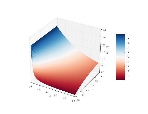
Let m𝑚m be the MGF of the log-likelihood, it is given by

m(α,β)=n=0βnn!Φn(α),𝑚𝛼𝛽superscriptsubscript𝑛0superscript𝛽𝑛𝑛subscriptΦ𝑛𝛼\displaystyle m(\alpha,\beta)=\sum_{n=0}^{\infty}\frac{\beta^{n}}{n!}\Phi_{n}(\alpha),

from which it follows that

m(α,β)α𝑚𝛼𝛽𝛼\displaystyle\frac{\partial m(\alpha,\beta)}{\partial\alpha} =\displaystyle= β(n=0βn+1(n+1)!Φn+1(α))Φ1(α)m(α,β)𝛽superscriptsubscript𝑛0superscript𝛽𝑛1𝑛1subscriptΦ𝑛1𝛼subscriptΦ1𝛼𝑚𝛼𝛽\displaystyle\frac{\partial}{\partial\beta}\left(\sum_{n=0}^{\infty}\frac{\beta^{n+1}}{(n+1)!}\Phi_{n+1}(\alpha)\right)-\Phi_{1}(\alpha)m(\alpha,\beta)
=\displaystyle= β(n=0βnn!Φn(α)β00!Φ0(α))Φ1(α)m(α,β)𝛽superscriptsubscript𝑛0superscript𝛽𝑛𝑛subscriptΦ𝑛𝛼superscript𝛽00subscriptΦ0𝛼subscriptΦ1𝛼𝑚𝛼𝛽\displaystyle\frac{\partial}{\partial\beta}\left(\sum_{n=0}^{\infty}\frac{\beta^{n}}{n!}\Phi_{n}(\alpha)-\frac{\beta^{0}}{0!}\Phi_{0}(\alpha)\right)-\Phi_{1}(\alpha)m(\alpha,\beta)
=\displaystyle= β(n=0βnn!Φn(α))Φ1(α)m(α,β).𝛽superscriptsubscript𝑛0superscript𝛽𝑛𝑛subscriptΦ𝑛𝛼subscriptΦ1𝛼𝑚𝛼𝛽\displaystyle\frac{\partial}{\partial\beta}\left(\sum_{n=0}^{\infty}\frac{\beta^{n}}{n!}\Phi_{n}(\alpha)\right)-\Phi_{1}(\alpha)m(\alpha,\beta).

The governing equation of the MGF is the following first order partial differential equation (PDE)

m(α,β)α=m(α,β)βΦ1(α)m(α,β),for(α,β)]0,1]×]0,Tβ].\displaystyle\frac{\partial m(\alpha,\beta)}{\partial\alpha}=\frac{\partial m(\alpha,\beta)}{\partial\beta}-\Phi_{1}(\alpha)m(\alpha,\beta),\quad\hbox{for}\quad(\alpha,\beta)\in]0,1]\times]0,T_{\beta}]. (35)

Equation (35) is a nonlinear advection-reaction equation that has to be equipped with a suitable boundary condition either at α=0𝛼0\alpha=0, α=1𝛼1\alpha=1, or β=0𝛽0\beta=0 to form a wellposed initial-value problem (IVP). Subsequently, applying the method of characteristics suffices to come up with the unique solution m𝑚m.

4.2.2 Admissible initial conditions

In this step, we enumerate all the initial conditions that can be assigned to (35) and aligned with our objective of not-sampling from any transition distribution, even less from the posterior one. Typically, we interpret the properties of MGF to arrive at the following conditions:

  • Initial value of MGF at β=0𝛽0\beta=0:

    m(α,0)=Φ0(α)=1.𝑚𝛼0subscriptΦ0𝛼1\displaystyle m(\alpha,0)=\Phi_{0}(\alpha)=1.
  • Initial value of MGF at the prior stage:

    m(0,β)𝑚0𝛽\displaystyle m(0,\beta) =\displaystyle= n=0βnn!Φn(0)=n=0βnn!𝔼𝜽|𝒀;α=0[lognp(𝒀|𝜽)]=n=0βnn!𝔼[lognp(𝒀|𝜽)]superscriptsubscript𝑛0superscript𝛽𝑛𝑛subscriptΦ𝑛0superscriptsubscript𝑛0superscript𝛽𝑛𝑛subscript𝔼conditional𝜽𝒀𝛼0delimited-[]superscript𝑛𝑝conditional𝒀𝜽superscriptsubscript𝑛0superscript𝛽𝑛𝑛𝔼delimited-[]superscript𝑛𝑝conditional𝒀𝜽\displaystyle\sum_{n=0}^{\infty}\frac{\beta^{n}}{n!}\Phi_{n}(0)=\sum_{n=0}^{\infty}\frac{\beta^{n}}{n!}\mathbb{E}_{\bm{\theta}|\bm{Y};\alpha=0}\left[\log^{n}p(\bm{Y}|\bm{\theta})\right]=\sum_{n=0}^{\infty}\frac{\beta^{n}}{n!}\mathbb{E}\left[\log^{n}p(\bm{Y}|\bm{\theta})\right]
    =\displaystyle= n=0𝔼[βnn!lognp(𝒀|𝜽)]=n=0𝔼[(βlogp(𝒀|𝜽))nn!].superscriptsubscript𝑛0𝔼delimited-[]superscript𝛽𝑛𝑛superscript𝑛𝑝conditional𝒀𝜽superscriptsubscript𝑛0𝔼delimited-[]superscript𝛽𝑝conditional𝒀𝜽𝑛𝑛\displaystyle\sum_{n=0}^{\infty}\mathbb{E}\left[\frac{\beta^{n}}{n!}\log^{n}p(\bm{Y}|\bm{\theta})\right]=\sum_{n=0}^{\infty}\mathbb{E}\left[\frac{\left(\beta\log p(\bm{Y}|\bm{\theta})\right)^{n}}{n!}\right].

    Let Xn(ω)=(βlogp(𝒀|𝜽(ω)))nn!subscript𝑋𝑛𝜔superscript𝛽𝑝conditional𝒀𝜽𝜔𝑛𝑛X_{n}(\omega)=\frac{\left(\beta\log p(\bm{Y}|\bm{\theta}(\omega))\right)^{n}}{n!} with ωΩ𝜔Ω\omega\in\Omega, as we consider a single observation setting for the likelihood, the inequality |Xn|βnn!subscript𝑋𝑛superscript𝛽𝑛𝑛|X_{n}|\leq\frac{\beta^{n}}{n!} holds almost everywhere, for all n𝑛n. It is obvious that the series of general terms βnn!superscript𝛽𝑛𝑛\frac{\beta^{n}}{n!} is a Taylor series, and obviously convergent. Consequently, we can interchange the integration 𝔼𝔼\mathbb{E} and the summation over non-negative integer n𝑛n of the mesurable function Xnsubscript𝑋𝑛X_{n}, that is

    m(0,β)=𝔼[n=0(βlogp(𝒀|𝜽))nn!]=𝔼[exp(βlogp(𝒀|𝜽))]=𝔼[pβ(𝒀|𝜽)].𝑚0𝛽𝔼delimited-[]superscriptsubscript𝑛0superscript𝛽𝑝conditional𝒀𝜽𝑛𝑛𝔼delimited-[]𝛽𝑝conditional𝒀𝜽𝔼delimited-[]superscript𝑝𝛽conditional𝒀𝜽\displaystyle m(0,\beta)=\mathbb{E}\left[\sum_{n=0}^{\infty}\frac{\left(\beta\log p(\bm{Y}|\bm{\theta})\right)^{n}}{n!}\right]=\mathbb{E}\left[\exp\left(\beta\log p(\bm{Y}|\bm{\theta})\right)\right]=\mathbb{E}\left[p^{\beta}(\bm{Y}|\bm{\theta})\right].

Looking for the initial condition at α=1𝛼1\alpha=1 results in m(1,β)=𝔼𝜽|𝒀;α=1[pβ(𝒀|𝜽)]𝑚1𝛽subscript𝔼conditional𝜽𝒀𝛼1delimited-[]superscript𝑝𝛽conditional𝒀𝜽m(1,\beta)=\mathbb{E}_{\bm{\theta}|\bm{Y};\alpha=1}\left[p^{\beta}(\bm{Y}|\bm{\theta})\right] and requires sampling from the posterior PDF, which we aim to avoid in this work. Roughly speaking, we shall deal with two candidates m(α,0)=1𝑚𝛼01m(\alpha,0)=1 and m(0,β)=𝔼[pβ(𝒀|𝜽)]𝑚0𝛽𝔼delimited-[]superscript𝑝𝛽conditional𝒀𝜽m(0,\beta)=\mathbb{E}\left[p^{\beta}(\bm{Y}|\bm{\theta})\right] as initial condition to complete the MGF equation.

4.2.3 Solving the MGF equation

We now investigate the analytical resolution of the MGF equation (35) in the domain ]0,1]×]0,+[]0,1]\times]0,+\infty[ with initial condition m(α,0)=1𝑚𝛼01m(\alpha,0)=1 or m(0,β)=𝔼[pβ(𝒀|𝜽)]𝑚0𝛽𝔼delimited-[]superscript𝑝𝛽conditional𝒀𝜽m(0,\beta)=\mathbb{E}\left[p^{\beta}(\bm{Y}|\bm{\theta})\right]. We consider the function F𝐹F, for the change of variable, given by

F(α,β)=m(α,β)exp(0αΦ1(τ)dτ).𝐹𝛼𝛽𝑚𝛼𝛽superscriptsubscript0𝛼subscriptΦ1𝜏d𝜏\displaystyle F(\alpha,\beta)=m(\alpha,\beta)\exp\left(\int_{0}^{\alpha}\Phi_{1}(\tau)\hbox{d}\tau\right).

Differentiating with respect to α𝛼\alpha and to β𝛽\beta (by applying the Leibniz integral rule) gives respectively

Fα𝐹𝛼\displaystyle\frac{\partial F}{\partial\alpha} =\displaystyle= mαexp(0αΦ1(τ)dτ)+(α0αΦ1(τ)dτ)m(α,β)exp(0αΦ1(τ)dτ)𝑚𝛼superscriptsubscript0𝛼subscriptΦ1𝜏d𝜏𝛼superscriptsubscript0𝛼subscriptΦ1𝜏d𝜏𝑚𝛼𝛽superscriptsubscript0𝛼subscriptΦ1𝜏d𝜏\displaystyle\frac{\partial m}{\partial\alpha}\exp\left(\int_{0}^{\alpha}\Phi_{1}(\tau)\hbox{d}\tau\right)+\left(\frac{\partial}{\partial\alpha}\int_{0}^{\alpha}\Phi_{1}(\tau)\hbox{d}\tau\right)m(\alpha,\beta)\exp\left(\int_{0}^{\alpha}\Phi_{1}(\tau)\hbox{d}\tau\right)
=\displaystyle= mαexp(0αΦ1(τ)dτ)+Φ1(α)m(t,α)exp(0αΦ1(τ)dτ)𝑚𝛼superscriptsubscript0𝛼subscriptΦ1𝜏d𝜏subscriptΦ1𝛼𝑚𝑡𝛼superscriptsubscript0𝛼subscriptΦ1𝜏d𝜏\displaystyle\frac{\partial m}{\partial\alpha}\exp\left(\int_{0}^{\alpha}\Phi_{1}(\tau)\hbox{d}\tau\right)+\Phi_{1}(\alpha)m(t,\alpha)\exp\left(\int_{0}^{\alpha}\Phi_{1}(\tau)\hbox{d}\tau\right)
=\displaystyle= (mα+Φ1(α)m(α,β))exp(0αΦ1(τ)dτ),𝑚𝛼subscriptΦ1𝛼𝑚𝛼𝛽superscriptsubscript0𝛼subscriptΦ1𝜏d𝜏\displaystyle\left(\frac{\partial m}{\partial\alpha}+\Phi_{1}(\alpha)m(\alpha,\beta)\right)\exp\left(\int_{0}^{\alpha}\Phi_{1}(\tau)\hbox{d}\tau\right),

and

Fβ=mβexp(0αΦ1(τ)dτ).𝐹𝛽𝑚𝛽superscriptsubscript0𝛼subscriptΦ1𝜏d𝜏\displaystyle\frac{\partial F}{\partial\beta}=\frac{\partial m}{\partial\beta}\exp\left(\int_{0}^{\alpha}\Phi_{1}(\tau)\hbox{d}\tau\right).

Plugging the MGF equation (35), it is seen that F𝐹F statifies the simpler equation

FαFβ=0,𝐹𝛼𝐹𝛽0\displaystyle\frac{\partial F}{\partial\alpha}-\frac{\partial F}{\partial\beta}=0, (36)

that has to be equipped with initial condition associated with one of the admissible initial conditions of (35) discussed in 4.2.2.

We examine the initial condition to mark out a well-posed IVP governing F𝐹F. The differential equation (36) with initial condition F0(α)subscript𝐹0𝛼F_{0}(\alpha), given by

F0(α)subscript𝐹0𝛼\displaystyle F_{0}(\alpha) =\displaystyle= F(0,α)𝐹0𝛼\displaystyle F(0,\alpha)
=\displaystyle= m(α,0)exp(0αΦ1(τ)dτ)𝑚𝛼0superscriptsubscript0𝛼subscriptΦ1𝜏d𝜏\displaystyle m(\alpha,0)\exp\left(\int_{0}^{\alpha}\Phi_{1}(\tau)\hbox{d}\tau\right)
=\displaystyle= exp(0αΦ1(τ)dτ),superscriptsubscript0𝛼subscriptΦ1𝜏d𝜏\displaystyle\exp\left(\int_{0}^{\alpha}\Phi_{1}(\tau)\hbox{d}\tau\right),

gives an ill-posed IVP in the Hadamard sense as it admits an infinity of solutions. However, the differential equation (36) with initial condition F0(β)superscript𝐹0𝛽F^{0}(\beta), given by

F0(β)superscript𝐹0𝛽\displaystyle F^{0}(\beta) =\displaystyle= m(0,β)𝑚0𝛽\displaystyle m(0,\beta)

has an unique solution of the form F(α,β)=m(0,β+α)𝐹𝛼𝛽𝑚0𝛽𝛼F(\alpha,\beta)=m(0,\beta+\alpha). From now on, we drop the initial condition m(α,0)=1𝑚𝛼01m(\alpha,0)=1 and the MGF equation refers to (35) and the initial condition m(0,β)=𝔼[pβ(𝒀|𝜽)]𝑚0𝛽𝔼delimited-[]superscript𝑝𝛽conditional𝒀𝜽m(0,\beta)=\mathbb{E}\left[p^{\beta}(\bm{Y}|\bm{\theta})\right], which together have a unique solution given by

m(α,β)=𝔼[pα+β(𝒀|𝜽)]exp(0αΦ1(τ)dτ).𝑚𝛼𝛽𝔼delimited-[]superscript𝑝𝛼𝛽conditional𝒀𝜽superscriptsubscript0𝛼subscriptΦ1𝜏d𝜏\displaystyle m(\alpha,\beta)=\mathbb{E}\left[p^{\alpha+\beta}(\bm{Y}|\bm{\theta})\right]\exp\left(-\int_{0}^{\alpha}\Phi_{1}(\tau)\hbox{d}\tau\right). (37)

4.2.4 Tractable formulation of the expected deviance

By definition of the MGF m𝑚m, the expected deviance Φ1subscriptΦ1\Phi_{1} is the derivative of m𝑚m with respect to β𝛽\beta evaluated at β=0𝛽0\beta=0,

Φ1(α)subscriptΦ1𝛼\displaystyle\Phi_{1}(\alpha) =\displaystyle= m(α,β)β|β=0evaluated-at𝑚𝛼𝛽𝛽𝛽0\displaystyle\frac{\partial m(\alpha,\beta)}{\partial\beta}\Big{|}_{\beta=0}
=\displaystyle= 𝔼[pα+β(𝒀|𝜽)]β|β=0exp(0αΦ1(τ)dτ)evaluated-at𝔼delimited-[]superscript𝑝𝛼𝛽conditional𝒀𝜽𝛽𝛽0superscriptsubscript0𝛼subscriptΦ1𝜏d𝜏\displaystyle\frac{\partial\mathbb{E}\left[p^{\alpha+\beta}(\bm{Y}|\bm{\theta})\right]}{\partial\beta}\Big{|}_{\beta=0}\,\exp\left(-\int_{0}^{\alpha}\Phi_{1}(\tau)\hbox{d}\tau\right)
=\displaystyle= 𝔼[logp(𝒀|𝜽)pα+β(𝒀|𝜽)]|β=0exp(0αΦ1(τ)dτ)evaluated-at𝔼delimited-[]𝑝conditional𝒀𝜽superscript𝑝𝛼𝛽conditional𝒀𝜽𝛽0superscriptsubscript0𝛼subscriptΦ1𝜏d𝜏\displaystyle\mathbb{E}\left[\log p(\bm{Y}|\bm{\theta})\,p^{\alpha+\beta}(\bm{Y}|\bm{\theta})\right]\Big{|}_{\beta=0}\exp\left(-\int_{0}^{\alpha}\Phi_{1}(\tau)\hbox{d}\tau\right)
=\displaystyle= 𝔼[logp(𝒀|𝜽)pα(𝒀|𝜽)]exp(0αΦ1(τ)dτ).𝔼delimited-[]𝑝conditional𝒀𝜽superscript𝑝𝛼conditional𝒀𝜽superscriptsubscript0𝛼subscriptΦ1𝜏d𝜏\displaystyle\mathbb{E}\left[\log p(\bm{Y}|\bm{\theta})\,p^{\alpha}(\bm{Y}|\bm{\theta})\right]\exp\left(-\int_{0}^{\alpha}\Phi_{1}(\tau)\hbox{d}\tau\right).

We let hh denote the tractile function depending on the tempering variable

h(α)=𝔼[logp(𝒀|𝜽)pα(𝒀|𝜽)],𝛼𝔼delimited-[]𝑝conditional𝒀𝜽superscript𝑝𝛼conditional𝒀𝜽\displaystyle h(\alpha)=\mathbb{E}\left[\log p(\bm{Y}|\bm{\theta})\,p^{\alpha}(\bm{Y}|\bm{\theta})\right],

the expected deviance Φ1subscriptΦ1\Phi_{1} is therefore solution of the nonlinear integral equation

Φ1(α)=h(α)exp(0αΦ1(τ)dτ).subscriptΦ1𝛼𝛼superscriptsubscript0𝛼subscriptΦ1𝜏d𝜏\displaystyle\Phi_{1}(\alpha)=h(\alpha)\exp\left(-\int_{0}^{\alpha}\Phi_{1}(\tau)\hbox{d}\tau\right). (38)

At this stage, numerical methods for solving integral equations can be applied to (38) to compute efficiently the expected deviance in a tempering grid, 0=α0α1αNα=10subscript𝛼0subscript𝛼1subscript𝛼subscript𝑁𝛼10=\alpha_{0}\leq\alpha_{1}\leq\cdots\leq\alpha_{N_{{}_{\alpha}}}=1, of Nα+1subscript𝑁𝛼1N_{{}_{\alpha}}+1 points. Nevertheless, we push forward towards a closed form of Φ1subscriptΦ1\Phi_{1} by differentiating (38) with respect to the tempering variable, by writing

Φ1α(α)subscriptΦ1𝛼𝛼\displaystyle\frac{\partial\Phi_{1}}{\partial\alpha}(\alpha) =\displaystyle= h(α)αexp(0αΦ1(τ)dτ)h(α)Φ1(α)exp(0αΦ1(τ)dτ)𝛼𝛼superscriptsubscript0𝛼subscriptΦ1𝜏d𝜏𝛼subscriptΦ1𝛼superscriptsubscript0𝛼subscriptΦ1𝜏d𝜏\displaystyle\frac{\partial h(\alpha)}{\partial\alpha}\exp\left(-\int_{0}^{\alpha}\Phi_{1}(\tau)\hbox{d}\tau\right)-h(\alpha)\Phi_{1}(\alpha)\exp\left(-\int_{0}^{\alpha}\Phi_{1}(\tau)\hbox{d}\tau\right)
=\displaystyle= h(α)α1h(α)(h(α)exp(0αΦ1(τ)dτ))Φ1(α)(h(α)exp(0αΦ1(τ)dτ))𝛼𝛼1𝛼𝛼superscriptsubscript0𝛼subscriptΦ1𝜏d𝜏subscriptΦ1𝛼𝛼superscriptsubscript0𝛼subscriptΦ1𝜏d𝜏\displaystyle\frac{\partial h(\alpha)}{\partial\alpha}\frac{1}{h(\alpha)}\left(h(\alpha)\exp\left(-\int_{0}^{\alpha}\Phi_{1}(\tau)\hbox{d}\tau\right)\right)-\Phi_{1}(\alpha)\left(h(\alpha)\exp\left(-\int_{0}^{\alpha}\Phi_{1}(\tau)\hbox{d}\tau\right)\right)
=\displaystyle= h(α)α1h(α)Φ1(α)Φ1(α)Φ1(α)𝛼𝛼1𝛼subscriptΦ1𝛼subscriptΦ1𝛼subscriptΦ1𝛼\displaystyle\frac{\partial h(\alpha)}{\partial\alpha}\frac{1}{h(\alpha)}\Phi_{1}(\alpha)-\Phi_{1}(\alpha)\Phi_{1}(\alpha)
=\displaystyle= h(α)α1h(α)Φ1(α)Φ12(α).𝛼𝛼1𝛼subscriptΦ1𝛼superscriptsubscriptΦ12𝛼\displaystyle\frac{\partial h(\alpha)}{\partial\alpha}\frac{1}{h(\alpha)}\Phi_{1}(\alpha)-\Phi_{1}^{2}(\alpha).

We find that the expected deviance is governed by a differential Bernouilli equation of second-type given by

{Φ1(α)=h(α)h(α)Φ1(α)Φ12(α)for0<α1,Φ1(0)=𝔼[logp(𝒀|𝜽)],casesformulae-sequencesuperscriptsubscriptΦ1𝛼superscript𝛼𝛼subscriptΦ1𝛼superscriptsubscriptΦ12𝛼for0𝛼1missing-subexpressionmissing-subexpressionmissing-subexpressionmissing-subexpressionmissing-subexpressionsubscriptΦ10𝔼delimited-[]𝑝conditional𝒀𝜽missing-subexpressionmissing-subexpression\displaystyle\left\{\begin{array}[]{lll}\Phi_{1}^{\prime}(\alpha)=\frac{h^{\prime}(\alpha)}{h(\alpha)}\Phi_{1}(\alpha)-\Phi_{1}^{2}(\alpha)\quad\hbox{for}\quad 0<\alpha\leq 1,\\ \\ \Phi_{1}(0)=\mathbb{E}\left[\log p(\bm{Y}|\bm{\theta})\right],\end{array}\right. (42)

with solution in the form

Φ1(α)=h(α)1+0αh(τ)dτ.subscriptΦ1𝛼𝛼1superscriptsubscript0𝛼𝜏d𝜏\displaystyle\Phi_{1}(\alpha)=\frac{h(\alpha)}{1+\displaystyle{\int_{0}^{\alpha}h(\tau)\hbox{d}\tau}}.

To gain clarity, we summarize the analysis presented in Section 4.2 in the following theorem.

Theorem 5.

The power-posterior distribution π(𝛉|𝐘;α)𝜋conditional𝛉𝐘𝛼\pi(\bm{\theta}|\bm{Y};\alpha) exists and is given by

π(𝜽|𝒀;α)=π(𝜽)pα(𝒀|𝜽)exp(0α𝔼𝜽|𝒀;τ[logp(𝒀|𝜽)]dτ)forα[0,1],formulae-sequence𝜋conditional𝜽𝒀𝛼𝜋𝜽superscript𝑝𝛼conditional𝒀𝜽superscriptsubscript0𝛼subscript𝔼conditional𝜽𝒀𝜏delimited-[]𝑝conditional𝒀𝜽d𝜏for𝛼01\displaystyle\pi(\bm{\theta}|\bm{Y};\alpha)=\pi(\bm{\theta})p^{\alpha}(\bm{Y}|\bm{\theta})\exp\left(-\int_{0}^{\alpha}\mathbb{E}_{\bm{\theta}|\bm{Y};\tau}\left[\log p(\bm{Y}|\bm{\theta})\right]\hbox{d}\tau\right)\quad\hbox{for}\quad\alpha\in[0,1], (43)

where the expected deviance is

𝔼𝜽|𝒀;α[logp(𝒀|𝜽)]=h(α)1+0αh(τ)dτ.subscript𝔼conditional𝜽𝒀𝛼delimited-[]𝑝conditional𝒀𝜽𝛼1superscriptsubscript0𝛼𝜏d𝜏\displaystyle\mathbb{E}_{\bm{\theta}|\bm{Y};\alpha}\left[\log p(\bm{Y}|\bm{\theta})\right]=\frac{h(\alpha)}{1+\displaystyle{\int_{0}^{\alpha}h(\tau)\hbox{d}\tau}}. (44)

Computing the power posterior distribution demands forward evaluations only for approximating Φ1(0)subscriptΦ10\Phi_{1}(0). The tractability, through (44), provides the expected deviance 𝔼𝜽|𝒀;α[logp(𝒀|𝜽)]=Φ1(α)subscript𝔼conditional𝜽𝒀𝛼delimited-[]𝑝conditional𝒀𝜽subscriptΦ1𝛼\mathbb{E}_{\bm{\theta}|\bm{Y};\alpha}\left[\log p(\bm{Y}|\bm{\theta})\right]=\Phi_{1}(\alpha) at any stage without any extra evaluations of the forward model 𝒈𝒈\bm{g}. In the next section, we justify the setting of (44) in term of computational stability and perform numerical experiments.

5 Numerical results

We conduct numerical results to assess the applicability and the practical aspect of our approach of computing the transition distributions while holding back evaluations of the forward model at the prior stage. Notations 𝒰𝒰\mathcal{U}, 𝒩𝒩\mathcal{N} and ΓΓ\Gamma refer to the uniform, normal and Gamma distributions, respectively. We present three numerical examples, the first is a one-dimensional linear model with Gaussian measurement errors where an explicit form of the expected deviance and of the tractile function hh allow to perform a detailed error analysis. The second example deals with a source inversion problem where the measurement errors are in a more realistic setting and are incorporated in the likelihood function using the Wasserstein distance. The third example is a challenging problem of multimodal inversion of a two-dimensional parameter.

5.1 Scaling domain and implementation

In the case of no interest in the transition distributions, the integral at (21) sums from 00 to 111 and can be casted as the expectation, with respect to the joint distribution π(𝜽,α)𝜋𝜽𝛼\pi(\bm{\theta},\alpha) of (𝜽,α)𝜽𝛼\left(\bm{\theta},\alpha\right), of the ratio of the log-likelihood over the distribution of the tempering parameter 𝔼𝜽,α|𝒀[logp(𝒀|𝜽)p(α)]subscript𝔼𝜽conditional𝛼𝒀delimited-[]𝑝conditional𝒀𝜽𝑝𝛼\mathbb{E}_{\bm{\theta},\alpha|\bm{Y}}\left[\frac{\log p(\bm{Y}|\bm{\theta})}{p(\alpha)}\right]. The total computational bias of that formulation copies only the model bias, generated for evaluating the forward model 𝒈𝒈\bm{g}, but requires the distribution p(α)𝑝𝛼p(\alpha) as given. The design of such unbiased estimators with MCMC methods, to compute the normalizing constant, has been addressed in [17, 30].

In the second instance, one would look at the expected deviance as the ratio of the expected values with respect to the prior PDF; Φ1(α)=𝔼[pα(𝒀|𝜽)logp(𝒀|𝜽)]𝔼[p(𝒀|𝜽)]subscriptΦ1𝛼𝔼delimited-[]superscript𝑝𝛼conditional𝒀𝜽𝑝conditional𝒀𝜽𝔼delimited-[]𝑝conditional𝒀𝜽\Phi_{1}(\alpha)=\frac{\mathbb{E}\left[p^{\alpha}(\bm{Y}|\bm{\theta})\log p(\bm{Y}|\bm{\theta})\right]}{\mathbb{E}\left[p(\bm{Y}|\bm{\theta})\right]}. As the numerator and the denominator have different scales of the likelihood, that formulation is likely unstable numerically because its ratio scale promotes numerical underflow even for small likelihood function (p(𝒀|𝜽)1𝑝conditional𝒀𝜽1p(\bm{Y}|\bm{\theta})\leq 1).

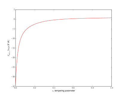
Refer to caption
Figure 1: scaling domain

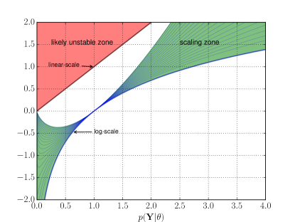
A crucial asset of the thermodynamic identity is that the expected deviance is on the logarithmic scale of the likelihood, which provides an unconditional numerical stability. That feature has been explored to advance MCMC methods in many ways in devising paths to access the posterior PDF (or in other terms in approximating the Bayes factor), see for instance [15, 27]. We believe that the logarithmic scale remains the best in terms of numerical stability despite the intractability issue and the intensive computational cost when it comes to profile transition distributions. One main purpose of this work is to avoid evaluations of the forward model 𝒈𝒈\bm{g} at transition stages, that subsequently induces the computational tractability. We also seek to preserve the numerical stability in the computation of the expected deviance. Rather than adopting a fixed scale of the likelihood function, our approach sweeps a scaling zone when computing the expected deviance. The scale changes from the log scale of the likelihood to the linear-log scale of the likelihood when α𝛼\alpha varies from 00 to 111. Although we fabricate our approach wih the assymption of p(𝒀|𝜽)1𝑝conditional𝒀𝜽1p(\bm{Y}|\bm{\theta})\leq 1 at a number of steps in the theoretical derivation, it is worth to mention that when α𝛼\alpha approaches 111 with large likelihood function (p(𝒀|𝜽)1much-greater-than𝑝conditional𝒀𝜽1p(\bm{Y}|\bm{\theta})\gg 1), the ratio scale of the expected deviance reduces drastically the risk of numerical instability due to the fact that the numerator and the denominator have the same scale in the likelihood function. In Figure 1, we schematize the scaling zone sweeping by the computation of the expected deviance Φ1(α)subscriptΦ1𝛼\Phi_{1}(\alpha) for α[0,1]𝛼01\alpha\in[0,1], the likely unstable zone, and the log scale.

Input:
Data𝒀Data𝒀\displaystyle\hbox{Data}\quad\bm{Y}
forward model𝒈forward model𝒈\displaystyle\hbox{forward model}\quad\bm{g}
tempering gridpoints{α0,α1,,αNα}tempering gridpointssubscript𝛼0subscript𝛼1subscript𝛼subscript𝑁𝛼\displaystyle\hbox{tempering gridpoints}\quad\{\alpha_{0},\alpha_{1},\cdots,\alpha_{N_{{}_{\tiny{\alpha}}}}\}
Output: Φ1(αk)subscriptΦ1subscript𝛼𝑘\Phi_{1}(\alpha_{k}) for k=0,,Nα𝑘0subscript𝑁𝛼k=0,\cdots,{N_{{}_{\tiny{\alpha}}}}
1 Generate 𝜽1,,𝜽Nsubscript𝜽1subscript𝜽𝑁\bm{\theta}_{1},\cdots,\bm{\theta}_{{}_{N}} from π(𝜽)𝜋𝜽\pi(\bm{\theta})
2 Evaluate 𝒈(𝜽1),,𝒈(𝜽N)𝒈subscript𝜽1𝒈subscript𝜽𝑁\bm{g}(\bm{\theta}_{1}),\cdots,\bm{g}(\bm{\theta}_{{}_{N}})
3 Evaluate logp(𝒀|𝜽n)𝑝conditional𝒀subscript𝜽𝑛\log p(\bm{Y}|\bm{\theta}_{n}) for n=1,,N𝑛1𝑁n=1,\cdots,N
4 Approximate h(α0):=𝔼[logp(𝒀|𝜽)]assignsubscript𝛼0𝔼delimited-[]𝑝conditional𝒀𝜽h(\alpha_{0}):=\mathbb{E}\left[\log p(\bm{Y}|\bm{\theta})\right], set (α0):=0assignPlanck-constant-over-2-pisubscript𝛼00\hbar(\alpha_{0}):=0
5 for k in {1,,Nα}1subscript𝑁𝛼\{1,\cdots,{N_{{}_{\tiny{\alpha}}}}\} do
6       Evaluate pαk(𝒀|𝜽n)superscript𝑝subscript𝛼𝑘conditional𝒀subscript𝜽𝑛p^{\alpha_{k}}(\bm{Y}|\bm{\theta}_{n}) for n=1,,N𝑛1𝑁n=1,\cdots,N
7       Approximate h(αk):=𝔼[pαk(𝒀|𝜽)logp(𝒀|𝜽)]assignsubscript𝛼𝑘𝔼delimited-[]superscript𝑝subscript𝛼𝑘conditional𝒀𝜽𝑝conditional𝒀𝜽h(\alpha_{k}):=\mathbb{E}\left[p^{\alpha_{k}}(\bm{Y}|\bm{\theta})\log p(\bm{Y}|\bm{\theta})\right]
8       Approximate (αk):=(αk1)+αk1αkh(τ)dτassignPlanck-constant-over-2-pisubscript𝛼𝑘Planck-constant-over-2-pisubscript𝛼𝑘1superscriptsubscriptsubscript𝛼𝑘1subscript𝛼𝑘𝜏d𝜏\hbar(\alpha_{k}):=\hbar(\alpha_{k-1})+\displaystyle{\int_{\alpha_{k-1}}^{\alpha_{k}}h(\tau)\hbox{d}\tau}
9       Evaluate Φ1(αk):=h(αk)1+(αk)assignsubscriptΦ1subscript𝛼𝑘subscript𝛼𝑘1Planck-constant-over-2-pisubscript𝛼𝑘\Phi_{1}(\alpha_{k}):=\displaystyle{\frac{h(\alpha_{k})}{1+\hbar(\alpha_{k})}}
Algorithm 1 Computation of Φ1subscriptΦ1\Phi_{1}

The Algorithm 1 summarizes the numerical approximation of the expected deviance for a given grid (αk)0kNαsubscriptsubscript𝛼𝑘0𝑘subscript𝑁𝛼\left(\alpha_{k}\right)_{0\leq k\leq N_{\alpha}}. Only N𝑁N evaluations of 𝒈𝒈\bm{g} at the prior stage suffice to compute the expected deviance Φ1subscriptΦ1\Phi_{1} at any stage αksubscript𝛼𝑘\alpha_{k}, including the posterior one (k=Nα𝑘subscript𝑁𝛼k=N_{\alpha}). That induces the tractability of the power posterior PDFs. In this work, the expected values at steps 4 and 7 in algorithm 1 are approximated using the Monte Carlo sampling, while the Simpson quadrature is employed for the local integration, from αk1subscript𝛼𝑘1\alpha_{k-1} to αksubscript𝛼𝑘\alpha_{k}, of the tractile function hh at step 8. Next, we present numerical experiments that cover only the method bias (bias generated by the tempering quadrature at step 8 in algorithm 1) since the evaluation of the forward model 𝒈𝒈\bm{g}, in each of the three examples, does not require a numerical discretization.

5.2 Example 1: A linear algebraic model

We consider an algebraic one-dimensional linear model, where the expected deviance Φ1subscriptΦ1\Phi_{1} and the tractile function hh can be computed analytically, given by

y=Aθ+ϵ.𝑦𝐴𝜃italic-ϵy=A\theta+\epsilon. (45)

Here our prior belief in the parameter of interest is characterized by a normal PDF, θ𝒩(1,σp2)similar-to𝜃𝒩1superscriptsubscript𝜎𝑝2\theta\sim\mathcal{N}\left(1,\sigma_{p}^{2}\right) and we consider that the observational noise for the data is Gaussian as well, i.e. ϵ𝒩(0,σϵ2)similar-toitalic-ϵ𝒩0superscriptsubscript𝜎italic-ϵ2\epsilon\sim\mathcal{N}\left(0,\sigma_{\epsilon}^{2}\right), which leads to a likelihood function of the form p(y|θ)=(2πσϵ2)1/2exp(12(yAθ)2σϵ2)𝑝conditional𝑦𝜃superscript2𝜋superscriptsubscript𝜎italic-ϵ21212superscript𝑦𝐴𝜃2superscriptsubscript𝜎italic-ϵ2p(y|\theta)=(2\pi\sigma_{\epsilon}^{2})^{-1/2}\exp\left(-\frac{1}{2}\frac{(y-A\theta)^{2}}{\sigma_{\epsilon}^{2}}\right). Let σα2=A2σp2α+σϵ2superscriptsubscript𝜎𝛼2superscript𝐴2superscriptsubscript𝜎𝑝2𝛼superscriptsubscript𝜎italic-ϵ2\sigma_{\alpha}^{2}=A^{2}\sigma_{p}^{2}\alpha+\sigma_{\epsilon}^{2}, we find that the expected deviance and the tractile function are, respectively, given by

𝔼θ|y;α[logp(y|θ)]subscript𝔼conditional𝜃𝑦𝛼delimited-[]𝑝conditional𝑦𝜃\displaystyle\mathbb{E}_{\theta|y;\alpha}\left[\log p(y|\theta)\right] =\displaystyle= 12(log(2πσϵ2)+A2σp2σα2+(yA)2σϵ2σα4),122𝜋superscriptsubscript𝜎italic-ϵ2superscript𝐴2superscriptsubscript𝜎𝑝2superscriptsubscript𝜎𝛼2superscript𝑦𝐴2superscriptsubscript𝜎italic-ϵ2superscriptsubscript𝜎𝛼4\displaystyle-\frac{1}{2}\left(\log\left(2\pi\sigma_{\epsilon}^{2}\right)+\frac{A^{2}\sigma_{p}^{2}}{\sigma_{\alpha}^{2}}+\frac{\left(y-A\right)^{2}\sigma_{\epsilon}^{2}}{\sigma_{\alpha}^{4}}\right),
h(α)𝛼\displaystyle h(\alpha) =\displaystyle= 12(2πσϵ2)α/2(log(2πσϵ2)+A2σp2σα2+(yA)2σϵ2σα4)exp(α2(yA)2σα2).12superscript2𝜋superscriptsubscript𝜎italic-ϵ2𝛼22𝜋superscriptsubscript𝜎italic-ϵ2superscript𝐴2superscriptsubscript𝜎𝑝2superscriptsubscript𝜎𝛼2superscript𝑦𝐴2superscriptsubscript𝜎italic-ϵ2superscriptsubscript𝜎𝛼4𝛼2superscript𝑦𝐴2superscriptsubscript𝜎𝛼2\displaystyle-\frac{1}{2}\left(2\pi\sigma_{\epsilon}^{2}\right)^{-\alpha/2}\left(\log\left(2\pi\sigma_{\epsilon}^{2}\right)+\frac{A^{2}\sigma_{p}^{2}}{\sigma_{\alpha}^{2}}+\frac{\left(y-A\right)^{2}\sigma_{\epsilon}^{2}}{\sigma_{\alpha}^{4}}\right)\exp\left(-\frac{\alpha}{2}\frac{(y-A)^{2}}{\sigma_{\alpha}^{2}}\right).

The synthetic data sample is acquired from the ”true” value θt=1.1subscript𝜃𝑡1.1\theta_{t}=1.1 with measurement errors diffusion coefficient of σϵ2=4.0superscriptsubscript𝜎italic-ϵ24.0\sigma_{\epsilon}^{2}=4.0.

Refer to caption
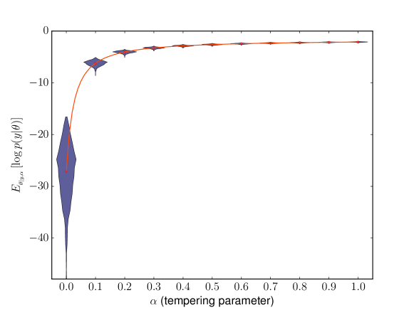
Figure 2: (Example 1) Distribution of the expected deviance and its expectation with respect to the evidence for the data model (45) with A=101𝐴101A=101 and σϵ2=4.0superscriptsubscript𝜎italic-ϵ24.0\sigma_{\epsilon}^{2}=4.0, σp2=102superscriptsubscript𝜎𝑝2superscript102\sigma_{p}^{2}=10^{-2}.

In Figure 2, we represent the expected deviance in term of the tempering parameter, and its expectation with respect to a data sample of size 103superscript10310^{3}, where the tractile function hh is approximated by Monte Carlo sampling with 103superscript10310^{3} samples. We also plot the distribution of the expected deviance at ten tempering points. The main observation here is the important variance reduction from the prior (α=0𝛼0\alpha=0) to the posterior (α=1𝛼1\alpha=1). As statement of this significant outcome, we observe that it is now possible to accurately estimate statistics with very few data, under the posterior distribution, with evaluations of 𝒈𝒈\bm{g} performed at the prior stage.

Refer to caption
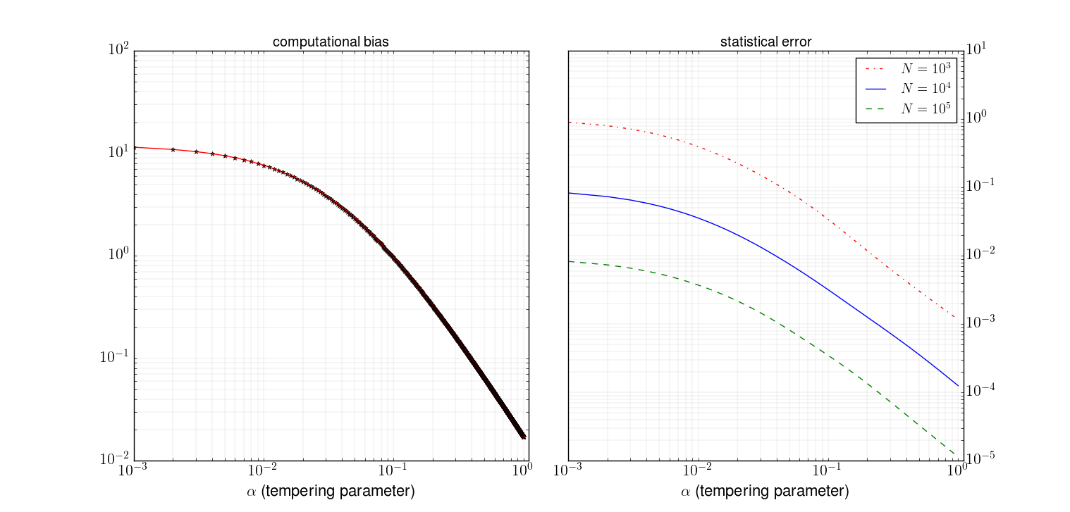
Figure 3: (Example 1) Error analysis

Figure 3 depicts the variations of the computational bias with respect to the tempering parameter and the statistical error for differents N𝑁N, number of random variables generated from the prior, in the Monte Carlo sampling to estimate h(α)𝛼h(\alpha). The computational bias is approximated as the mean value over a dataset of size 103superscript10310^{3} of the absolute value of the exact 𝔼θ|y;α[logp(y|θ)]subscript𝔼conditional𝜃𝑦𝛼delimited-[]𝑝conditional𝑦𝜃\mathbb{E}_{\theta|y;\alpha}\left[\log p(y|\theta)\right] minus the expected deviance at (44) evaluated with the exact tractile function h(α)𝛼h(\alpha). Here, the bias is purely associated to the tempering quadrature error, and is improving by order 103superscript10310^{-3} from the prior to the posterior. We let the statistical error be the L2superscript𝐿2L^{2} norm of the difference between the exact deviance and the expected deviance (44) evaluated with hN(α)subscript𝑁𝛼h_{{}_{N}}(\alpha), where hN(α)subscript𝑁𝛼h_{{}_{N}}(\alpha) is the Monte Carlo approximation of the tractile function with N𝑁N samples. The statistical error plot (right-plot, Figure 3) allows to quantify the variance reduction observed in Figure 2. From each of the three cases, N=103,104,105𝑁superscript103superscript104superscript105N=10^{3},10^{4},10^{5}, one can see a significant variance reduction of the expected deviance from 103superscript10310^{3} at the prior stage to 111 at the posterior one.

5.3 Example 2: Source inversion with Wasserstein metric-based likelihood

We now consider the example of source inversion problem, treated in [26], where an initial wave pulse propagates with a constant speed. The mathematical governing equation is the one-dimensional wave equation

{utt(t,x)uxx(t,x)=0in]0,T]×,u(0,x)=u0(x,𝜽)in,ut(0,x)=0in.\displaystyle\left\{\begin{array}[]{ll}\displaystyle{u_{tt}(t,x)-u_{xx}(t,x)=0}&\displaystyle{\text{in}\quad]0,T]\times\mathbb{R},\vspace{0.1cm}}\\ \displaystyle{u(0,x)=u^{0}(x,\bm{\theta})}&\displaystyle{\text{in}\quad\mathbb{R},\vspace{0.1cm}}\\ \displaystyle{u_{t}(0,x)=0}&\displaystyle{\text{in}\quad\mathbb{R}.}\end{array}\right. (49)

We aim to assess how our continuation inversion approach performs for complicated structure of the measurement errors composed with a multiplicative and additive noises. We consider an initial pulse of the form

u0(x,𝜽)=aexp(100(xx00.5)2)+aexp(100(xx0)2)+aexp(100(xx0+0.5)2)superscript𝑢0𝑥𝜽𝑎100superscript𝑥subscript𝑥00.52𝑎100superscript𝑥subscript𝑥02𝑎100superscript𝑥subscript𝑥00.52\displaystyle u^{0}(x,\bm{\theta})=a\exp\left(-100(x-x_{0}-0.5)^{2}\right)+a\exp\left(-100(x-x_{0})^{2}\right)+a\exp\left(-100(x-x_{0}+0.5)^{2}\right)

from an unknown location x0subscript𝑥0x_{0} with an unknown amplitude a𝑎a that we aim to learn continuously from the prior stage to the posterior one. Therefore the parameter of interest is 𝜽=(x0,a)𝜽subscript𝑥0𝑎\bm{\theta}=(x_{0},a). The forward model g𝑔g is the solution of (49) that is in the form

g(t,x,𝜽)=defu(t,x)=12u0(xt,𝜽)+12u0(x+t,𝜽).superscriptdef𝑔𝑡𝑥𝜽𝑢𝑡𝑥12superscript𝑢0𝑥𝑡𝜽12superscript𝑢0𝑥𝑡𝜽\displaystyle g(t,x,\bm{\theta})\mathrel{\stackrel{{\scriptstyle\makebox[0.0pt]{\mbox{\tiny def}}}}{{=}}}u(t,x)=\frac{1}{2}u^{0}(x-t,\bm{\theta})+\frac{1}{2}u^{0}(x+t,\bm{\theta}). (50)

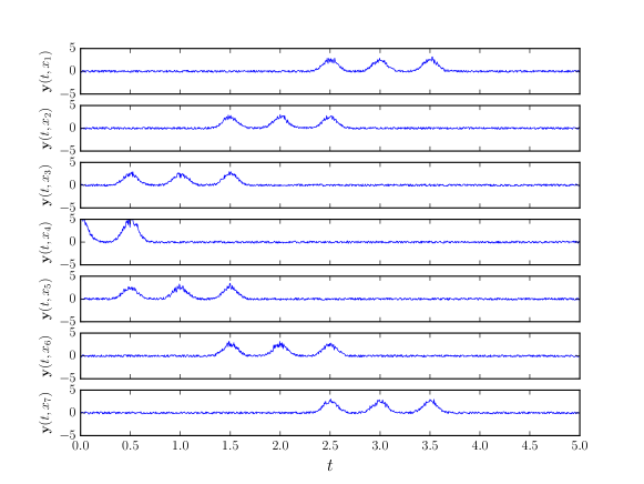
Seven receivers, Nr=7subscript𝑁𝑟7N_{r}=7, are placed at locations x1=3subscript𝑥13x_{1}=-3, x2=2subscript𝑥22x_{2}=-2, x3=1subscript𝑥31x_{3}=-1, x4=0subscript𝑥40x_{4}=0, x5=1subscript𝑥51x_{5}=1, x6=2subscript𝑥62x_{6}=2 and x7=3subscript𝑥73x_{7}=3 to record polluted discrete-time signal 𝒚rsubscript𝒚𝑟\bm{y}_{r} over the time interval [0,T]0𝑇[0,T] at NTsubscript𝑁𝑇N_{{}_{T}} time-steps tk=k1NT1Tsubscript𝑡𝑘𝑘1subscript𝑁𝑇1𝑇t_{k}=\frac{k-1}{N_{{}_{T}}-1}T, k=1,,NT𝑘1subscript𝑁𝑇k=1,\cdots,N_{{}_{T}}. The data 𝒀𝒀\bm{Y} is represented as 𝒀={𝒚1,,𝒚Nr}𝒀subscript𝒚1subscript𝒚subscript𝑁𝑟\bm{Y}=\left\{\bm{y}_{1},\cdots,\bm{y}_{N_{r}}\right\}, where the rthsuperscript𝑟𝑡r^{th} receiver is counting the responses y(tk,xr)𝑦subscript𝑡𝑘subscript𝑥𝑟y(t_{k},x_{r}) at all the NTsubscript𝑁𝑇N_{{}_{T}} time-steps, 𝒚r=(y(tk,xr))1kNTsubscript𝒚𝑟subscript𝑦subscript𝑡𝑘subscript𝑥𝑟1𝑘subscript𝑁𝑇\bm{y}_{r}=\left(y(t_{k},x_{r})\right)_{1\leq k\leq N_{{}_{T}}} where

y(tk,xr)=ϵkr(1)g(tk,xr,𝜽t)+ϵkr(2),𝑦subscript𝑡𝑘subscript𝑥𝑟superscriptsubscriptitalic-ϵ𝑘𝑟1𝑔subscript𝑡𝑘subscript𝑥𝑟subscript𝜽𝑡superscriptsubscriptitalic-ϵ𝑘𝑟2\displaystyle y(t_{k},x_{r})=\epsilon_{kr}^{(1)}g(t_{k},x_{r},\bm{\theta}_{t})+\epsilon_{kr}^{(2)}, (51)

with ϵkr(1)Γ(60,1/60)similar-tosuperscriptsubscriptitalic-ϵ𝑘𝑟1Γ60160\epsilon_{kr}^{(1)}\sim\Gamma(60,1/60) and ϵkr(2)𝒰(0.25,0.25)similar-tosuperscriptsubscriptitalic-ϵ𝑘𝑟2𝒰0.250.25\epsilon_{kr}^{(2)}\sim\mathcal{U}(-0.25,0.25). In the numerical experiment, we consider T=5𝑇5T=5.

Refer to caption
Figure 4: (Example 2) Recorded signal 𝒀𝒀\bm{Y} at the seven receivers with NT=1001subscript𝑁𝑇1001N_{{}_{T}}=1001.

To compute the power posterior distributions of 𝜽𝜽\bm{\theta}, we consider the likelihood function as follows

p(𝒀|𝜽)=sNTexp(sr=1Nr𝐝𝐢𝐬W(𝒚r,𝒈r(𝜽))),𝑝conditional𝒀𝜽superscript𝑠subscript𝑁𝑇𝑠superscriptsubscript𝑟1subscript𝑁𝑟subscript𝐝𝐢𝐬𝑊subscript𝒚𝑟subscript𝒈𝑟𝜽\displaystyle p(\bm{Y}|\bm{\theta})=s^{N_{{}_{T}}}\exp\left(-s\sum_{r=1}^{N_{r}}\operatorname{\bf dis}_{{}_{W}}\left(\bm{y}_{r},\bm{g}_{r}(\bm{\theta})\right)\right), (52)

where 𝒈r(𝜽)subscript𝒈𝑟𝜽\bm{g}_{r}(\bm{\theta}) gathers the NTsubscript𝑁𝑇N_{{}_{T}} outputs of the forward model, 𝒈r(𝜽)=(g(tk,xr,𝜽))1kNTsubscript𝒈𝑟𝜽subscript𝑔subscript𝑡𝑘subscript𝑥𝑟𝜽1𝑘subscript𝑁𝑇\bm{g}_{r}(\bm{\theta})=\left(g(t_{k},x_{r},\bm{\theta})\right)_{1\leq k\leq N_{{}_{T}}} evaluated with the random parameter 𝜽𝜽\bm{\theta}, and 𝐝𝐢𝐬Wsubscript𝐝𝐢𝐬𝑊\operatorname{\bf dis}_{{}_{W}} stands for the quadratic Wasserstein distance. The errors dispersion parameter s𝑠s is also not available to us and is assumed random, sΓ(1,0.1)similar-to𝑠Γ10.1s\sim\Gamma(1,0.1).

Refer to caption
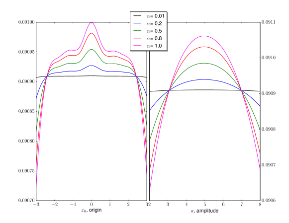
Figure 5: (Example 2) Marginal transition distributions of the origin x0subscript𝑥0x_{0} (left-plot) and the amplitude a𝑎a (right-plot) conditioned with a recorded signal of length NT=101subscript𝑁𝑇101N_{{}_{T}}=101 at the seven receivers.

Figure 5 presents the marginal power posterior distributions of the location x0subscript𝑥0x_{0} (left plot) and of the amplitude a𝑎a (right plot) at different tempering points. The simulation is performed with a single synthetic data generated with the ”true” location and ”true”pulse amplitude 𝜽t=(0.0,0.5)subscript𝜽𝑡0.00.5\bm{\theta}_{t}=(0.0,0.5), with signal length of NT=101subscript𝑁𝑇101N_{{}_{T}}=101. The tractile function hh is approximated with the Monte Carlo sampling with 102superscript10210^{2} samples. Our continuation method handles perfectly that complex noise structure as the marginal power posteriors concentrate around the true values when the tempering parameter goes to 111.

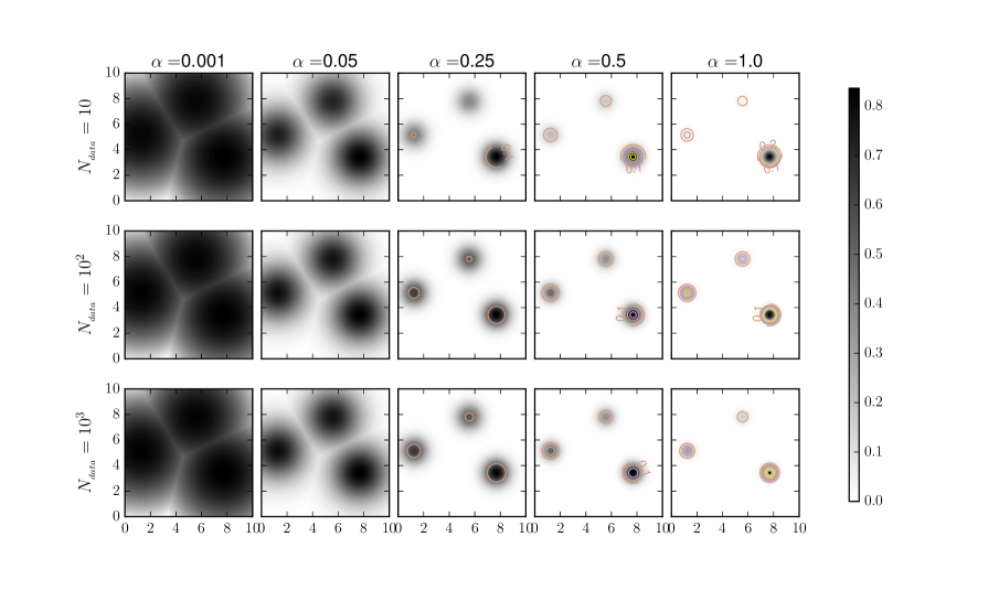
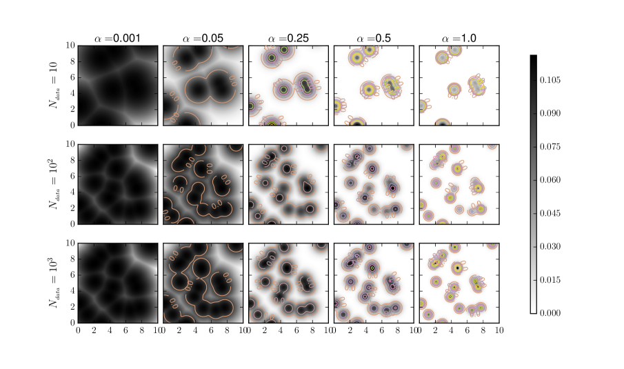
5.4 Example 3: Bivariate multimodal inversion

In this example we confront our approach, in terms of capturing the evolution of the distribution from the prior to the posterior, to a mixture of M𝑀M two-dimensional Gaussians. Let us consider the data representation

𝒀=𝜽+ϵ,𝒀𝜽bold-italic-ϵ\displaystyle\bm{Y}=\bm{\theta}+\bm{\epsilon}, (53)

where the measurement errors is Gaussian, ϵ𝒩(𝟎,σ2𝑰2)similar-tobold-italic-ϵ𝒩0superscript𝜎2subscript𝑰2\bm{\epsilon}\sim\mathcal{N}\left(\bm{0},\sigma^{2}\bm{I}_{2}\right), 𝑰2subscript𝑰2\bm{I}_{2} is the 2×2222\times 2 unit matrix, and 𝜽𝜽\bm{\theta} is drawn form the bivariate uniform prior, 𝜽𝒰([0,10])×𝒰([0,10])similar-to𝜽𝒰010𝒰010\bm{\theta}\sim\mathcal{U}\left([0,10]\right)\times\mathcal{U}\left([0,10]\right). We consider a synthetic data, of size Ndatasubscript𝑁dataN_{{}_{\tiny{\hbox{data}}}}, collected from the categorical distribution of M𝑀M modes, 𝒀𝒩(𝜽t,σ2𝑰2)similar-to𝒀𝒩subscript𝜽𝑡superscript𝜎2subscript𝑰2\bm{Y}\sim\mathcal{N}\left(\bm{\theta}_{t},\sigma^{2}\bm{I}_{2}\right) with 𝜽t=𝝁1𝝁2𝝁Msubscript𝜽𝑡subscript𝝁1subscript𝝁2subscript𝝁𝑀\bm{\theta}_{t}=\bm{\mu}_{1}\vee\bm{\mu}_{2}\vee\cdots\vee\bm{\mu}_{M}, where \vee stands for the logical connective operator ”or inclusive”. This example is built on the multimodal simulation case treated for assessing advance classes of MCMC methods [21, 33]. The likelihood function has the form

p(𝒀|𝜽)=m=1Mp[w(𝒚m)=wm](𝒚m|𝜽)𝑝conditional𝒀𝜽superscriptsubscriptproduct𝑚1𝑀superscript𝑝delimited-[]𝑤subscript𝒚𝑚subscript𝑤𝑚conditionalsubscript𝒚𝑚𝜽\displaystyle p(\bm{Y}|\bm{\theta})=\prod_{m=1}^{M}p^{[w(\bm{y}_{m})=w_{m}]}(\bm{y}_{m}|\bm{\theta}) (54)

for a data 𝒀=(𝒚1,,𝒚M)𝒀subscript𝒚1subscript𝒚𝑀\bm{Y}=(\bm{y}_{1},\cdots,\bm{y}_{M}) sampled from 𝒀𝒩(𝜽t,σ2𝑰2)similar-to𝒀𝒩subscript𝜽𝑡superscript𝜎2subscript𝑰2\bm{Y}\sim\mathcal{N}\left(\bm{\theta}_{t},\sigma^{2}\bm{I}_{2}\right), where [=][\cdot=\cdot] represents the Iverson bracket, w(𝒚m)𝑤subscript𝒚𝑚w(\bm{y}_{m}) is the weight of 𝒚msubscript𝒚𝑚\bm{y}_{m}, and wmsubscript𝑤𝑚w_{m} is the assigned weight to the mode 𝝁msubscript𝝁𝑚\bm{\mu}_{m}, m=1,,M𝑚1𝑀m=1,\cdots,M.

Refer to caption
Figure 6: (Example 3) Expected deviance with respect to joint distribution of the parameter of interest and the data.

To demonstrate further the effectiveness of our proposed method, we investigate the ability of computing the expected deviance with respect to the joint distribution of the parameter of interest and the data. For Ndata=103subscript𝑁datasuperscript103N_{{}_{\tiny{\hbox{data}}}}=10^{3}, N=102𝑁superscript102N=10^{2}, we show in Figure 6 the evolution of the expected deviance in terms of the tempering parameter. The categorical distribution has M=3𝑀3M=3 modes in this numerical experiment with 𝝁1=(2.18,5.76)subscript𝝁12.185.76\bm{\mu}_{1}=(2.18,5.76), 𝝁2=(8.41,1.68)subscript𝝁28.411.68\bm{\mu}_{2}=(8.41,1.68) and 𝝁3=(5.54,6.86)subscript𝝁35.546.86\bm{\mu}_{3}=(5.54,6.86).

Refer to caption
Figure 7: (Example 3) Moments generating function surface in the unit square [0,1]×[0,1]0101[0,1]\times[0,1].

Using the same configuration: categorical distribution with three modes, Ndata=103subscript𝑁datasuperscript103N_{{}_{\tiny{\hbox{data}}}}=10^{3}, N=102𝑁superscript102N=10^{2}, we display the MGF for (α,β)[0,1]×[0,1]𝛼𝛽0101(\alpha,\beta)\in[0,1]\times[0,1] to stay consistent with the fact the MGF only exists for β[0,1]𝛽01\beta\in[0,1] and as our interest to the MGF is for small β𝛽\beta.

In multimodal inversion, one important observation when using the Bayesian approach is that all the modes might not be captured for small size datasets. We investigate this phenomena using our continuation approach by setting two different configurations. The first is a weighted categorical distribution with M=3𝑀3M=3 modes, where w1=0.3subscript𝑤10.3w_{1}=0.3, w2=0.5subscript𝑤20.5w_{2}=0.5 and w3=0.2subscript𝑤30.2w_{3}=0.2 (Figure 8). The second configuration deals with a categorical distribution with M=20𝑀20M=20, where wm=1/20subscript𝑤𝑚120w_{m}=1/20, for m=1,,20𝑚120m=1,\cdots,20 and the modes locations are collected from [21], where they are uniformly sampled from the prior π(𝜽)𝜋𝜽\pi(\bm{\theta}) and given by

𝝁1=(2.18,5.76),subscript𝝁12.185.76\displaystyle\bm{\mu}_{1}=(2.18,5.76), 𝝁6=(3.25,3.47),subscript𝝁63.253.47\displaystyle\bm{\mu}_{6}=(3.25,3.47), 𝝁11=(5.41,2.65),subscript𝝁115.412.65\displaystyle\bm{\mu}_{11}=(5.41,2.65), 𝝁16=(4.93,1.50),subscript𝝁164.931.50\displaystyle\bm{\mu}_{16}=(4.93,1.50),
𝝁2=(8.67,9.59),subscript𝝁28.679.59\displaystyle\bm{\mu}_{2}=(8.67,9.59), 𝝁7=(1.70,0.50),subscript𝝁71.700.50\displaystyle\bm{\mu}_{7}=(1.70,0.50), 𝝁12=(2.70,7.88),subscript𝝁122.707.88\displaystyle\bm{\mu}_{12}=(2.70,7.88), 𝝁17=(1.83,0.09),subscript𝝁171.830.09\displaystyle\bm{\mu}_{17}=(1.83,0.09),
𝝁3=(4.24,8.48),subscript𝝁34.248.48\displaystyle\bm{\mu}_{3}=(4.24,8.48), 𝝁8=(4.59,5.60),subscript𝝁84.595.60\displaystyle\bm{\mu}_{8}=(4.59,5.60), 𝝁13=(4.98,3.70),subscript𝝁134.983.70\displaystyle\bm{\mu}_{13}=(4.98,3.70), 𝝁18=(2.26,0.31),subscript𝝁182.260.31\displaystyle\bm{\mu}_{18}=(2.26,0.31),
𝝁4=(8.41,1.68),subscript𝝁48.411.68\displaystyle\bm{\mu}_{4}=(8.41,1.68), 𝝁9=(6.91,5.81),subscript𝝁96.915.81\displaystyle\bm{\mu}_{9}=(6.91,5.81), 𝝁14=(1.14,2.39),subscript𝝁141.142.39\displaystyle\bm{\mu}_{14}=(1.14,2.39), 𝝁19=(5.54,6.86),subscript𝝁195.546.86\displaystyle\bm{\mu}_{19}=(5.54,6.86),
𝝁5=(3.93,8.82),subscript𝝁53.938.82\displaystyle\bm{\mu}_{5}=(3.93,8.82), 𝝁10=(6.87,5.40),subscript𝝁106.875.40\displaystyle\bm{\mu}_{10}=(6.87,5.40), 𝝁15=(8.33,9.50),subscript𝝁158.339.50\displaystyle\bm{\mu}_{15}=(8.33,9.50), 𝝁20=(1.69,8.11).subscript𝝁201.698.11\displaystyle\bm{\mu}_{20}=(1.69,8.11).

Figures 8 and 9 are obtained with a Monte Carlo approximation of N=102𝑁superscript102N=10^{2} samples of the tractile function hh, and Simpson quadrature with 111111 gridpoints is used for the tempering quadrature between αksubscript𝛼𝑘\alpha_{k} and αk+1subscript𝛼𝑘1\alpha_{k+1}.

Refer to caption
Figure 8: (Example 3) Power posteriors distributions with three modes
Refer to caption
Figure 9: (Example 3) Power posteriors distributions with 20 modes

In Figures 8 and 9, we visualize the update of the distribution of the parameter of interest. For the first case, M=3𝑀3M=3, the power posterior distribution shows all the three modes at the earlier stage even for the small size dataset, and the distribution concentrates around the modes as the tempering parameter goes to 111. In Figure 9, our continuation approach exhibits, at the earlier stage, the effect of non-capturing all the modes for small size datasets. However, the number of captured modes increased with the dataset for the largest size.

6 Conclusions

We presented a continuation method for interpreting the posterior probability density function, as the terminal stage of a path of transition distribution functions between the prior and the posterior, for Bayesian inverse problems with exponential likelihood function. A mathematical analysis for the existence and the uniqueness of the transition distributions has been presented to support the consistency of our results. We managed to hold back all the evaluations of the forward model at the prior stage in the approximation of the transition distribution. That achieves the computational tractability of the posterior distribution in opposite to classical MCMC methods where the acceptance condition complicates the counting, a priori, of the number the forward model evaluations. The computational tractability was addressed through the tractability of the expected deviance using the moments generating function of the log-likelihood function. Our research has stressed the important potential of continuation methods for two of the three classes of uncertainty quantification tasks enumerated in [31].

The presented numerical results dealt with evaluations of simple forward models while for real-world applications the output of the forward model is typically obtained through numerical approximations of PDEs that require physical discretization, and therefore incorporates the model bias. One window scoping the improvement of this approach that we aim to investigate is the combination of the multilevel Monte Carlo method, for the approximation of the tractile function, with high precision quadrature schemes for the tempering quadrature.

One intriguing question coming up when observing the transition distributions is: Are the data goodness criteria, for parameter estimation problems, following the same updating rate when the tempering parameter varies from 00 to 111? Depending on the answer, one would either reduce the method bias in the computation of the data goodness criteria by considering an earlier tempering point as the final stage. Or one can design a hierarchical clustering algorithm on a dataset for the inferential strength in parameter estimation problems. Future work will also explore this aspect for the Kullback-Leibler divergence in the framework of Bayesian experimental design.

Acknowledgments

The author is grateful to Kody J. Law (Manchester University), Youssef Marzouk (MIT, Cambridge) and Raul Tempone (KAUST & Alexander von Humboldt Professor at RWTH Aachen University) for valuable discussions and comments.

References

  • [1] Appell, J. ”On revient toujours à son premier amour”: On the mathematical work of Espedito De Pascale. Communications in Applied Analysis 13, 4 (2009), 461–476.
  • [2] Appell, J., Diallo, O., and Zabrejko, P. On linear integro-differential equation of Barbashin type in spaces of continuous and measurable functions. Journal of Integral Equations and Applications 1, 2 (1988), 1–22.
  • [3] Appell, J., Kalitvin, A., and Zabrejko, P. Boundary value problems for integro-differential equations of Barbashin type. Journal of Integral Equations and Applications 6, 1 (1994), 1–30.
  • [4] Appell, J., Kalitvin, A., and Zabrejko, P. Partial integral operators and integro-differential equations: pure and applied mathematics. Chapman & Hall/CRC Pure and Applied Mathematics, 2000.
  • [5] Beck, J., Dia, B., Espath, L., Long, Q., and Tempone, R. Fast Bayesian experimental design: Laplace-based importance sampling for the expected information gain. Computer Methods in Applied Mechanics and Engineering 334 (2018), 523–553.
  • [6] Beck, J., Dia, B., Espath, L., and Tempone, R. Multilevel double loop Monte Carlo and stochastic collocation methods with importance sampling for Bayesian optimal experimental design. arXiv:1807.00653v2 (2018).
  • [7] Dashti, M., and Stuart, A. M. The Bayesian approach to inverse problem. Springer International Publishing Switzerland. R. Ghanem et al. (eds.), Handbook of Uncertainty Quantification (2017), 311–428.
  • [8] Earl, D., and Deem, M. Parallel tempering: Theory, applications, and new perspectives. Phys. Chem. Chem. Phys. 7 (2005), 3910–3916.
  • [9] Egozcue, J., Diaz-Barrero, J., and Pawlowsky-Glahn, V. Hilbert space of probability density functions based on Aitchison geometry. Acta Mathematica Sinica, English Series 22, 4 (2006), 1175–1182.
  • [10] Feng, C., and Marzouk, Y. A layered multiple importance sampling scheme for focused optimal Bayesian experimental design. arXiv:1903.11187v1 (2019).
  • [11] Francois, O., and Laval, G. Deviance information criteria for model selection in Approximate Bayesian Computation. Statistical Applications in Genetics and Molecular Biology 10, 1 (2011).
  • [12] Friel, N., Hurn, M., and Wyse, J. Improving power posterior estimation of statistical evidence. Statistics and Computing 24, 5 (September 2014), 709–723.
  • [13] Friel, N., and Pettitt, A. N. Marginal likelihood estimation via power posteriors. Journal of the Royal Statistical Society. Series B (Statistical Methodology) 70, 3 (2008), 589–607.
  • [14] Gangbo, W., and McCann, R. J. The geometry of optimal transportation. Acta Mathematica 177, 2 (1996), 113–161.
  • [15] Gelman, A., and Meng, X.-L. Simulating normalizing constants: From importance sampling to bridge sampling to path sampling. Statistical Science 13, 2 (1998), 163–185.
  • [16] Heng, J. On the use of transport and optimal control methods for Monte Carlo simulation. PhD thesis, University of Oxford, 2016.
  • [17] Jacob, P. E., O’Leary, J., and Atchadé, Y. F. Unbiased markov chain monte carlo with couplings. arXiv:1708.03625v5 (2019).
  • [18] Kalitvin, A. Some aspects of the theory of integro-differential Barbashin equations in function spaces. Journal of Mathematical Sciences 188, 3 (2013), 241–249.
  • [19] Kou, S., Zhou, Q., and Wong, W. Equi-energy sampler with applications in statistical inference and statistical mechanics. The Annals of Statistics 34, 4 (2006), 1581–1619.
  • [20] Lartillot, N., and Philippe, H. Computing Bayes factors using thermodynamic integration. Syst. Biol. 55, 2 (2006), 195–207.
  • [21] Lian, F., and Wong, W. Real-parameter evolutionary Monte Carlo with applications to bayesian mixture models. Journal of the American Statistical Association 96, 454 (2001), 653–666.
  • [22] Liu, P., Kim, B., Friesner, R. A., and Berne, B. J. Replica exchange with solute tempering: A method for sampling biological systems in explicit water. Proceedings of the National Academy of Sciences 102, 39 (2005), 13749–13754.
  • [23] Marzouk, Y., Moselhy, T., Parno, M., and Spantini, A. Sampling via measure transport: An introduction. Springer, Cham, 2006.
  • [24] Morzfeld, M., Day, M., Grout, R., Hengpau, G., Finsterle, S., and Bell, A. Iterative importance sampling algorithms for parameter estimation. SIAM J. Sci. Comput. 40, 2 (2018), B329–B352.
  • [25] Moselhy, T., and Marzouk, Y. Bayesian inference with optimal maps. Journal of Computational Physics 231, 23 (2012), 7815–7850.
  • [26] Motamed, M., and Appelo, D. Wasserstein metric-driven Bayesian inversion with applications to signal processing. International Journal for Uncertainty Quantification 9, 4 (2019), 395–414.
  • [27] Neal, R. M. Sampling from multimodal distributions using tempered transitions. Statistics and Computing 6, 4 (Dec 1996), 353–366.
  • [28] Reade, J. Eigenvalues of positive definite kernels. SIAM J. Math. Anal. 14, 1 (2006), 152–157.
  • [29] Reich, S., and Shin, S. On the consistency of ensemble transform filter formulations. Journal of Computational Dynamics 1, 1 (2014), 177–189.
  • [30] Rischard, M., Jacob, P. E., and Pillai, N. Unbiased estimation of log normalizing constants with applications to Bayesian cross-validation. arXiv:1810.01382v1 (2018).
  • [31] Rüde, U., Willcox, K., McInnes, L. C., and Sterck, H. D. Research and education in computational science and engineering. SIAM Review 60, 3 (2018), 707–754.
  • [32] Santin, G., and Schaback, R. Approximation of eigenfunctions in kernel-based spaces. Advances in Computational Mathematics 42, 4 (2016), 973–993.
  • [33] Stojkova, B. J. Bayesian methods for multi-modal posterior topologies. PhD thesis, Simon Fraser University, 2017.
  • [34] Stuart, A. M. Inverse problems: A Bayesian perspective. Acta Numerica 19 (2010), 451–559.
  • [35] Sugita, Y., and Okamoto, Y. Replica-exchange molecular dynamics method for protein folding. Chemical Physics Letters 314 (1999), 141–151.
  • [36] Syed, S., Bouchard-Côté, A., Deligiannidis, G., and Doucet, A. Non-reversible parallel tempering : A scalable highly parallel MCMC scheme. arXiv:1905.02939v2 (2019).
  • [37] Villani, C. Topics in optimal transportation, vol. 58. American Mathematical Society, Providence, Rhode Island, 2003.

Appendix A Proof of Theorem 4

The goal is to prove the existence and the uniqueness of solution for the Barbashin equation (20b). We introduce the abstract function v^^𝑣\hat{v} defined as

v^:[0,1]𝒮lαv^(α)=defv(α,).:^𝑣01absentsubscript𝒮𝑙𝛼absent^𝑣𝛼superscriptdef𝑣𝛼\displaystyle\hat{v}\colon\begin{aligned} [0,1]&\longrightarrow\mathcal{S}_{l}\\ \alpha&\longmapsto\hat{v}(\alpha)\mathrel{\stackrel{{\scriptstyle\makebox[0.0pt]{\mbox{\tiny def}}}}{{=}}}{v}(\alpha,\cdot).\end{aligned} (55)

Therefore, we can rewrite (20b) as an abstract Cauchy problem

dv^dα=A(α)v^(𝜽),d^𝑣d𝛼𝐴𝛼^𝑣𝜽\displaystyle\frac{\hbox{d}\hat{v}}{\hbox{d}\alpha}=A(\alpha)\hat{v}(\bm{\theta}), (56)

where v^(𝜽)=v^(α)(𝜽)^𝑣𝜽^𝑣𝛼𝜽\hat{v}(\bm{\theta})=\hat{v}(\alpha)(\bm{\theta}), the derivative dv^dαd^𝑣d𝛼\frac{\hbox{d}\hat{v}}{\hbox{d}\alpha} is in the Fréchet sense, and the Cauchy operator A𝐴A is the integral operator given by

A(α)v^(𝜽)=Θ(α,𝜽,𝜼,v^(𝜼))d𝜼.𝐴𝛼^𝑣𝜽subscriptΘ𝛼𝜽𝜼^𝑣𝜼d𝜼\displaystyle A(\alpha)\hat{v}(\bm{\theta})=\int_{\Theta}\mathcal{H}(\alpha,\bm{\theta},\bm{\eta},\hat{v}(\bm{\eta}))\hbox{d}\bm{\eta}. (57)

The classical solvability of (56) follows from the strong continuity of the integral operator

A:[0,1](𝒮)αA(α),:𝐴01absent𝒮𝛼absent𝐴𝛼\displaystyle A\colon\begin{aligned} [0,1]&\longrightarrow\mathcal{L}(\mathcal{S})\\ \alpha&\longmapsto A(\alpha),\end{aligned} (58)

where (𝒮l)subscript𝒮𝑙\mathcal{L}(\mathcal{S}_{l}) is the space of all bounded linear operators in the Banach space 𝒮lsubscript𝒮𝑙\mathcal{S}_{l}. Therefore we get the solvability since A𝐴A is strongly continuous in (𝒮l)subscript𝒮𝑙\mathcal{L}(\mathcal{S}_{l}) by construction. Indeed, let (αn)n>0subscriptsubscript𝛼𝑛𝑛0(\alpha_{n})_{n>0} be a sequence of real valued numbers in [0,1]01[0,1] that converges to α[0,1]𝛼01\alpha\in[0,1], and \|\cdot\|_{\mathcal{L}} be an appropriate norm defined in (𝒮l)subscript𝒮𝑙\mathcal{L}(\mathcal{S}_{l}), we have

A(αn)A(α)subscriptnorm𝐴subscript𝛼𝑛𝐴𝛼\displaystyle\left\|A(\alpha_{n})-A(\alpha)\right\|_{\mathcal{L}} =\displaystyle= |Θ(αn,𝜽,𝜼,v^(𝜼))(α,𝜽,𝜼,v^(𝜼))d𝜼|subscriptΘsubscript𝛼𝑛𝜽𝜼^𝑣𝜼𝛼𝜽𝜼^𝑣𝜼d𝜼\displaystyle|\int_{\Theta}\mathcal{H}(\alpha_{n},\bm{\theta},\bm{\eta},\hat{v}(\bm{\eta}))-\mathcal{H}(\alpha,\bm{\theta},\bm{\eta},\hat{v}(\bm{\eta}))\hbox{d}\bm{\eta}|
=\displaystyle= |Θ(αn,𝜽,𝜼,v^(αn)(𝜼))(α,𝜽,𝜼,v^(α)(𝜼))d𝜼|subscriptΘsubscript𝛼𝑛𝜽𝜼^𝑣subscript𝛼𝑛𝜼𝛼𝜽𝜼^𝑣𝛼𝜼d𝜼\displaystyle|\int_{\Theta}\mathcal{H}(\alpha_{n},\bm{\theta},\bm{\eta},\hat{v}(\alpha_{n})(\bm{\eta}))-\mathcal{H}(\alpha,\bm{\theta},\bm{\eta},\hat{v}(\alpha)(\bm{\eta}))\hbox{d}\bm{\eta}|
\displaystyle\leq Θ|(αn,𝜽,𝜼,v^(αn)(𝜼))(α,𝜽,𝜼,v^(α)(𝜼))|d𝜼subscriptΘsubscript𝛼𝑛𝜽𝜼^𝑣subscript𝛼𝑛𝜼𝛼𝜽𝜼^𝑣𝛼𝜼d𝜼\displaystyle\int_{\Theta}|\mathcal{H}(\alpha_{n},\bm{\theta},\bm{\eta},\hat{v}(\alpha_{n})(\bm{\eta}))-\mathcal{H}(\alpha,\bm{\theta},\bm{\eta},\hat{v}(\alpha)(\bm{\eta}))|\hbox{d}\bm{\eta}
\displaystyle\leq Θ|(αn,𝜽,𝜼,v^(αn)(𝜼))(α,𝜽,𝜼,v^(αn)(𝜼))|d𝜼subscriptΘsubscript𝛼𝑛𝜽𝜼^𝑣subscript𝛼𝑛𝜼𝛼𝜽𝜼^𝑣subscript𝛼𝑛𝜼d𝜼\displaystyle\int_{\Theta}|\mathcal{H}(\alpha_{n},\bm{\theta},\bm{\eta},\hat{v}(\alpha_{n})(\bm{\eta}))-\mathcal{H}(\alpha,\bm{\theta},\bm{\eta},\hat{v}(\alpha_{n})(\bm{\eta}))|\hbox{d}\bm{\eta}
+Θ|(α,𝜽,𝜼,v^(αn)(𝜼))(α,𝜽,𝜼,v^(α)(𝜼))|d𝜼subscriptΘ𝛼𝜽𝜼^𝑣subscript𝛼𝑛𝜼𝛼𝜽𝜼^𝑣𝛼𝜼d𝜼\displaystyle+\int_{\Theta}|\mathcal{H}(\alpha,\bm{\theta},\bm{\eta},\hat{v}(\alpha_{n})(\bm{\eta}))-\mathcal{H}(\alpha,\bm{\theta},\bm{\eta},\hat{v}(\alpha)(\bm{\eta}))|\hbox{d}\bm{\eta}

The functional v^^𝑣\hat{v} is continuous, and as 𝒈𝒈\bm{g} is assumed continuous with respect to 𝜽𝜽\bm{\theta}, the kernel \mathcal{H} is continuous. Therefore A𝐴A is strongly continuous. This completes the proof.

Appendix B Derivation of the kernel trace equations

We use the orthogonality condition (26) and the eigenvalue problem setting (27) to characterize the dynamics of the eigenvalue λnsubscript𝜆𝑛\lambda_{n}.

λn(α)subscript𝜆𝑛𝛼\displaystyle\lambda_{n}(\alpha) =\displaystyle= λn(α)knα(𝜽),knα(𝜽)αsubscript𝜆𝑛𝛼subscriptsubscriptsuperscript𝑘𝛼𝑛𝜽subscriptsuperscript𝑘𝛼𝑛𝜽𝛼\displaystyle\lambda_{n}(\alpha)\left\langle k^{\alpha}_{n}(\bm{\theta}),k^{\alpha}_{n}(\bm{\theta})\right\rangle_{\alpha}
=\displaystyle= λn(α)Θknα(𝜽)knα(𝜽)π(𝜽|𝒀;α)d𝜽subscript𝜆𝑛𝛼subscriptΘsubscriptsuperscript𝑘𝛼𝑛𝜽subscriptsuperscript𝑘𝛼𝑛𝜽𝜋conditional𝜽𝒀𝛼d𝜽\displaystyle\lambda_{n}(\alpha)\int_{\Theta}k^{\alpha}_{n}(\bm{\theta})k^{\alpha}_{n}(\bm{\theta})\pi(\bm{\theta}|\bm{Y};\alpha)\hbox{d}\bm{\theta}
=\displaystyle= Θknα(𝜽)λn(α)knα(𝜽)π(𝜽|𝒀;α)d𝜽subscriptΘsubscriptsuperscript𝑘𝛼𝑛𝜽subscript𝜆𝑛𝛼subscriptsuperscript𝑘𝛼𝑛𝜽𝜋conditional𝜽𝒀𝛼d𝜽\displaystyle\int_{\Theta}k^{\alpha}_{n}(\bm{\theta})\lambda_{n}(\alpha)k^{\alpha}_{n}(\bm{\theta})\pi(\bm{\theta}|\bm{Y};\alpha)\hbox{d}\bm{\theta}
=\displaystyle= Θknα(𝜽)Θ𝒦(α,𝜽,𝜼)knα(𝜼)π(𝜼|𝒀;α)d𝜼π(𝜽|𝒀;α)d𝜽.subscriptΘsubscriptsuperscript𝑘𝛼𝑛𝜽subscriptΘ𝒦𝛼𝜽𝜼subscriptsuperscript𝑘𝛼𝑛𝜼𝜋conditional𝜼𝒀𝛼d𝜼𝜋conditional𝜽𝒀𝛼d𝜽\displaystyle\int_{\Theta}k^{\alpha}_{n}(\bm{\theta})\int_{\Theta}\mathcal{K}(\alpha,\bm{\theta},\bm{\eta})k^{\alpha}_{n}(\bm{\eta})\pi(\bm{\eta}|\bm{Y};\alpha)\hbox{d}\bm{\eta}\;\pi(\bm{\theta}|\bm{Y};\alpha)\hbox{d}\bm{\theta}.

Differentiation with respect to the parameter α𝛼\alpha gives

λn(α)αsubscript𝜆𝑛𝛼𝛼\displaystyle\frac{\partial\lambda_{n}(\alpha)}{\partial\alpha} =\displaystyle= Θknα(𝜽)Θ𝒦(α,𝜽,𝜼)knα(𝜼)απ(𝜼|𝒀;α)d𝜼π(𝜽|𝒀;α)d𝜽subscriptΘsubscriptsuperscript𝑘𝛼𝑛𝜽subscriptΘ𝒦𝛼𝜽𝜼subscriptsuperscript𝑘𝛼𝑛𝜼𝛼𝜋conditional𝜼𝒀𝛼d𝜼𝜋conditional𝜽𝒀𝛼d𝜽\displaystyle\int_{\Theta}k^{\alpha}_{n}(\bm{\theta})\int_{\Theta}\mathcal{K}(\alpha,\bm{\theta},\bm{\eta})k^{\alpha}_{n}(\bm{\eta})\frac{\partial}{\partial\alpha}\pi(\bm{\eta}|\bm{Y};\alpha)\hbox{d}\bm{\eta}\;\pi(\bm{\theta}|\bm{Y};\alpha)\hbox{d}\bm{\theta}
+Θknα(𝜽)Θ𝒦(α,𝜽,𝜼)knα(𝜼)π(𝜼|𝒀;α)d𝜼απ(𝜽|𝒀;α)d𝜽,subscriptΘsubscriptsuperscript𝑘𝛼𝑛𝜽subscriptΘ𝒦𝛼𝜽𝜼subscriptsuperscript𝑘𝛼𝑛𝜼𝜋conditional𝜼𝒀𝛼d𝜼𝛼𝜋conditional𝜽𝒀𝛼d𝜽\displaystyle+\int_{\Theta}k^{\alpha}_{n}(\bm{\theta})\int_{\Theta}\mathcal{K}(\alpha,\bm{\theta},\bm{\eta})k^{\alpha}_{n}(\bm{\eta})\pi(\bm{\eta}|\bm{Y};\alpha)\hbox{d}\bm{\eta}\;\frac{\partial}{\partial\alpha}\pi(\bm{\theta}|\bm{Y};\alpha)\hbox{d}\bm{\theta},

yet from (4), we obtain

Θ𝒦(α,𝜽,𝜼)knα(𝜼)απ(𝜼|𝒀;α)d𝜼subscriptΘ𝒦𝛼𝜽𝜼subscriptsuperscript𝑘𝛼𝑛𝜼𝛼𝜋conditional𝜼𝒀𝛼d𝜼\displaystyle\int_{\Theta}\mathcal{K}(\alpha,\bm{\theta},\bm{\eta})k^{\alpha}_{n}(\bm{\eta})\frac{\partial}{\partial\alpha}\pi(\bm{\eta}|\bm{Y};\alpha)\hbox{d}\bm{\eta} =\displaystyle= Θlogp(𝒀|𝜼)𝒦(α,𝜽,𝜼)knα(𝜼)π(𝜼|𝒀;α)d𝜼subscriptΘ𝑝conditional𝒀𝜼𝒦𝛼𝜽𝜼subscriptsuperscript𝑘𝛼𝑛𝜼𝜋conditional𝜼𝒀𝛼d𝜼\displaystyle\int_{\Theta}\log p(\bm{Y}|\bm{\eta})\mathcal{K}(\alpha,\bm{\theta},\bm{\eta})k^{\alpha}_{n}(\bm{\eta})\pi(\bm{\eta}|\bm{Y};\alpha)\hbox{d}\bm{\eta}
𝔼𝜼|𝒀;α[logp(𝒀|𝜼)]Θ𝒦(α,𝜽,𝜼)knα(𝜼)π(𝜼|𝒀;α)d𝜼.subscript𝔼conditional𝜼𝒀𝛼delimited-[]𝑝conditional𝒀𝜼subscriptΘ𝒦𝛼𝜽𝜼subscriptsuperscript𝑘𝛼𝑛𝜼𝜋conditional𝜼𝒀𝛼d𝜼\displaystyle-\mathbb{E}_{\bm{\eta}|\bm{Y};\alpha}\left[\log p(\bm{Y}|\bm{\eta})\right]\int_{\Theta}\mathcal{K}(\alpha,\bm{\theta},\bm{\eta})k^{\alpha}_{n}(\bm{\eta})\pi(\bm{\eta}|\bm{Y};\alpha)\hbox{d}\bm{\eta}.

It follows that

I1subscript𝐼1\displaystyle I_{1} =defsuperscriptdef\displaystyle\mathrel{\stackrel{{\scriptstyle\makebox[0.0pt]{\mbox{\tiny def}}}}{{=}}} Θknα(𝜽)Θ𝒦(α,𝜽,𝜼)knα(𝜼)απ(𝜼|𝒀;α)d𝜼π(𝜽|𝒀;α)d𝜽subscriptΘsubscriptsuperscript𝑘𝛼𝑛𝜽subscriptΘ𝒦𝛼𝜽𝜼subscriptsuperscript𝑘𝛼𝑛𝜼𝛼𝜋conditional𝜼𝒀𝛼d𝜼𝜋conditional𝜽𝒀𝛼d𝜽\displaystyle\int_{\Theta}k^{\alpha}_{n}(\bm{\theta})\int_{\Theta}\mathcal{K}(\alpha,\bm{\theta},\bm{\eta})k^{\alpha}_{n}(\bm{\eta})\frac{\partial}{\partial\alpha}\pi(\bm{\eta}|\bm{Y};\alpha)\hbox{d}\bm{\eta}\;\pi(\bm{\theta}|\bm{Y};\alpha)\hbox{d}\bm{\theta}
=\displaystyle= Θknα(𝜽)Θlogp(𝒀|𝜼)𝒦(α,𝜽,𝜼)knα(𝜼)π(𝜼|𝒀;α)d𝜼π(𝜽|𝒀;α)d𝜽subscriptΘsubscriptsuperscript𝑘𝛼𝑛𝜽subscriptΘ𝑝conditional𝒀𝜼𝒦𝛼𝜽𝜼subscriptsuperscript𝑘𝛼𝑛𝜼𝜋conditional𝜼𝒀𝛼d𝜼𝜋conditional𝜽𝒀𝛼d𝜽\displaystyle\int_{\Theta}k^{\alpha}_{n}(\bm{\theta})\int_{\Theta}\log p(\bm{Y}|\bm{\eta})\mathcal{K}(\alpha,\bm{\theta},\bm{\eta})k^{\alpha}_{n}(\bm{\eta})\pi(\bm{\eta}|\bm{Y};\alpha)\hbox{d}\bm{\eta}\;\pi(\bm{\theta}|\bm{Y};\alpha)\hbox{d}\bm{\theta}
𝔼𝜼|𝒀;α[logp(𝒀|𝜼)]Θknα(𝜽)Θ𝒦(α,𝜽,𝜼)knα(𝜼)π(𝜼|𝒀;α)d𝜼π(𝜽|𝒀;α)d𝜽.subscript𝔼conditional𝜼𝒀𝛼delimited-[]𝑝conditional𝒀𝜼subscriptΘsubscriptsuperscript𝑘𝛼𝑛𝜽subscriptΘ𝒦𝛼𝜽𝜼subscriptsuperscript𝑘𝛼𝑛𝜼𝜋conditional𝜼𝒀𝛼d𝜼𝜋conditional𝜽𝒀𝛼d𝜽\displaystyle-\mathbb{E}_{\bm{\eta}|\bm{Y};\alpha}\left[\log p(\bm{Y}|\bm{\eta})\right]\int_{\Theta}k^{\alpha}_{n}(\bm{\theta})\int_{\Theta}\mathcal{K}(\alpha,\bm{\theta},\bm{\eta})k^{\alpha}_{n}(\bm{\eta})\pi(\bm{\eta}|\bm{Y};\alpha)\hbox{d}\bm{\eta}\;\pi(\bm{\theta}|\bm{Y};\alpha)\hbox{d}\bm{\theta}.
=\displaystyle= Θknα(𝜽)Θlogp(𝒀|𝜼)l=1λl(α)klα(𝜽)lkα(𝜼)knα(𝜼)π(𝜼|𝒀;α)d𝜼π(𝜽|𝒀;α)d𝜽subscriptΘsubscriptsuperscript𝑘𝛼𝑛𝜽subscriptΘ𝑝conditional𝒀𝜼superscriptsubscript𝑙1subscript𝜆𝑙𝛼superscriptsubscript𝑘𝑙𝛼𝜽superscriptsubscript𝑙𝑘𝛼𝜼subscriptsuperscript𝑘𝛼𝑛𝜼𝜋conditional𝜼𝒀𝛼d𝜼𝜋conditional𝜽𝒀𝛼d𝜽\displaystyle\int_{\Theta}k^{\alpha}_{n}(\bm{\theta})\int_{\Theta}\log p(\bm{Y}|\bm{\eta})\sum_{l=1}^{\infty}\lambda_{l}(\alpha)k_{l}^{\alpha}(\bm{\theta})l_{k}^{\alpha}(\bm{\eta})k^{\alpha}_{n}(\bm{\eta})\pi(\bm{\eta}|\bm{Y};\alpha)\hbox{d}\bm{\eta}\;\pi(\bm{\theta}|\bm{Y};\alpha)\hbox{d}\bm{\theta}
𝔼𝜼|𝒀;α[logp(𝒀|𝜼)]Θknα(𝜽)λn(α)knα(𝜽)π(𝜽|𝒀;α)d𝜽subscript𝔼conditional𝜼𝒀𝛼delimited-[]𝑝conditional𝒀𝜼subscriptΘsubscriptsuperscript𝑘𝛼𝑛𝜽subscript𝜆𝑛𝛼subscriptsuperscript𝑘𝛼𝑛𝜽𝜋conditional𝜽𝒀𝛼d𝜽\displaystyle-\mathbb{E}_{\bm{\eta}|\bm{Y};\alpha}\left[\log p(\bm{Y}|\bm{\eta})\right]\int_{\Theta}k^{\alpha}_{n}(\bm{\theta})\lambda_{n}(\alpha)k^{\alpha}_{n}(\bm{\theta})\;\pi(\bm{\theta}|\bm{Y};\alpha)\hbox{d}\bm{\theta}
=\displaystyle= l=1Θknα(𝜽)klα(𝜽)π(𝜽|𝒀;α)d𝜽Θlogp(𝒀|𝜼)λl(α)klα(𝜼)knα(𝜼)π(𝜼|𝒀;α)d𝜼superscriptsubscript𝑙1subscriptΘsubscriptsuperscript𝑘𝛼𝑛𝜽superscriptsubscript𝑘𝑙𝛼𝜽𝜋conditional𝜽𝒀𝛼d𝜽subscriptΘ𝑝conditional𝒀𝜼subscript𝜆𝑙𝛼superscriptsubscript𝑘𝑙𝛼𝜼subscriptsuperscript𝑘𝛼𝑛𝜼𝜋conditional𝜼𝒀𝛼d𝜼\displaystyle\sum_{l=1}^{\infty}\int_{\Theta}k^{\alpha}_{n}(\bm{\theta})k_{l}^{\alpha}(\bm{\theta})\;\pi(\bm{\theta}|\bm{Y};\alpha)\hbox{d}\bm{\theta}\int_{\Theta}\log p(\bm{Y}|\bm{\eta})\lambda_{l}(\alpha)k_{l}^{\alpha}(\bm{\eta})k^{\alpha}_{n}(\bm{\eta})\pi(\bm{\eta}|\bm{Y};\alpha)\hbox{d}\bm{\eta}
λn(α)𝔼𝜼|𝒀;α[logp(𝒀|𝜼)]subscript𝜆𝑛𝛼subscript𝔼conditional𝜼𝒀𝛼delimited-[]𝑝conditional𝒀𝜼\displaystyle-\lambda_{n}(\alpha)\mathbb{E}_{\bm{\eta}|\bm{Y};\alpha}\left[\log p(\bm{Y}|\bm{\eta})\right]
=\displaystyle= λn(α)Θlogp(𝒀|𝜼)knα(𝜼)knα(𝜼)π(𝜼|𝒀;α)d𝜼λn(α)𝔼𝜼|𝒀;α[logp(𝒀|𝜼)].subscript𝜆𝑛𝛼subscriptΘ𝑝conditional𝒀𝜼superscriptsubscript𝑘𝑛𝛼𝜼subscriptsuperscript𝑘𝛼𝑛𝜼𝜋conditional𝜼𝒀𝛼d𝜼subscript𝜆𝑛𝛼subscript𝔼conditional𝜼𝒀𝛼delimited-[]𝑝conditional𝒀𝜼\displaystyle\lambda_{n}(\alpha)\int_{\Theta}\log p(\bm{Y}|\bm{\eta})k_{n}^{\alpha}(\bm{\eta})k^{\alpha}_{n}(\bm{\eta})\pi(\bm{\eta}|\bm{Y};\alpha)\hbox{d}\bm{\eta}-\lambda_{n}(\alpha)\mathbb{E}_{\bm{\eta}|\bm{Y};\alpha}\left[\log p(\bm{Y}|\bm{\eta})\right].

Similarly

I2subscript𝐼2\displaystyle I_{2} =defsuperscriptdef\displaystyle\mathrel{\stackrel{{\scriptstyle\makebox[0.0pt]{\mbox{\tiny def}}}}{{=}}} Θknα(𝜽)Θ𝒦(α,𝜽,𝜼)knα(𝜼)π(𝜼|𝒀;α)d𝜼απ(𝜽|𝒀;α)d𝜽subscriptΘsubscriptsuperscript𝑘𝛼𝑛𝜽subscriptΘ𝒦𝛼𝜽𝜼subscriptsuperscript𝑘𝛼𝑛𝜼𝜋conditional𝜼𝒀𝛼d𝜼𝛼𝜋conditional𝜽𝒀𝛼d𝜽\displaystyle\int_{\Theta}k^{\alpha}_{n}(\bm{\theta})\int_{\Theta}\mathcal{K}(\alpha,\bm{\theta},\bm{\eta})k^{\alpha}_{n}(\bm{\eta})\pi(\bm{\eta}|\bm{Y};\alpha)\hbox{d}\bm{\eta}\;\frac{\partial}{\partial\alpha}\pi(\bm{\theta}|\bm{Y};\alpha)\hbox{d}\bm{\theta}
=\displaystyle= λn(α)Θlogp(𝒀|𝜼)knα(𝜼)knα(𝜼)π(𝜼|𝒀;α)d𝜼λn(α)𝔼𝜼|𝒀;α[logp(𝒀|𝜼)].subscript𝜆𝑛𝛼subscriptΘ𝑝conditional𝒀𝜼superscriptsubscript𝑘𝑛𝛼𝜼subscriptsuperscript𝑘𝛼𝑛𝜼𝜋conditional𝜼𝒀𝛼d𝜼subscript𝜆𝑛𝛼subscript𝔼conditional𝜼𝒀𝛼delimited-[]𝑝conditional𝒀𝜼\displaystyle\lambda_{n}(\alpha)\int_{\Theta}\log p(\bm{Y}|\bm{\eta})k_{n}^{\alpha}(\bm{\eta})k^{\alpha}_{n}(\bm{\eta})\pi(\bm{\eta}|\bm{Y};\alpha)\hbox{d}\bm{\eta}-\lambda_{n}(\alpha)\mathbb{E}_{\bm{\eta}|\bm{Y};\alpha}\left[\log p(\bm{Y}|\bm{\eta})\right].

Therefore, the dynamics of an eigenvalue is

λn(α)α=2λn(α)Θlogp(𝒀|𝜼)knα(𝜼)knα(𝜼)π(𝜼|𝒀;α)d𝜼2λn(α)𝔼𝜼|𝒀;α[logp(𝒀|𝜼)].subscript𝜆𝑛𝛼𝛼2subscript𝜆𝑛𝛼subscriptΘ𝑝conditional𝒀𝜼superscriptsubscript𝑘𝑛𝛼𝜼subscriptsuperscript𝑘𝛼𝑛𝜼𝜋conditional𝜼𝒀𝛼d𝜼2subscript𝜆𝑛𝛼subscript𝔼conditional𝜼𝒀𝛼delimited-[]𝑝conditional𝒀𝜼\displaystyle\frac{\partial\lambda_{n}(\alpha)}{\partial\alpha}=2\lambda_{n}(\alpha)\int_{\Theta}\log p(\bm{Y}|\bm{\eta})k_{n}^{\alpha}(\bm{\eta})k^{\alpha}_{n}(\bm{\eta})\pi(\bm{\eta}|\bm{Y};\alpha)\hbox{d}\bm{\eta}-2\lambda_{n}(\alpha)\mathbb{E}_{\bm{\eta}|\bm{Y};\alpha}\left[\log p(\bm{Y}|\bm{\eta})\right]. (59)

Using

logp(𝒀|𝜼)=log(C)s𝒦(α,𝜼,𝜼)and𝔼𝜼|𝒀;α[logp(𝒀|𝜼)]𝑝conditional𝒀𝜼C𝑠𝒦𝛼𝜼𝜼andsubscript𝔼conditional𝜼𝒀𝛼delimited-[]𝑝conditional𝒀𝜼\displaystyle\log p(\bm{Y}|\bm{\eta})=\log(\text{C})-s\mathcal{K}(\alpha,\bm{\eta},\bm{\eta})\quad\hbox{and}\quad\mathbb{E}_{\bm{\eta}|\bm{Y};\alpha}\left[\log p(\bm{Y}|\bm{\eta})\right] =\displaystyle= log(C)sΘ𝒦(α,𝜼,𝜼)π(𝜽|𝒀;α)d𝜼C𝑠subscriptΘ𝒦𝛼𝜼𝜼𝜋conditional𝜽𝒀𝛼d𝜼\displaystyle\log(\text{C})-s\int_{\Theta}\mathcal{K}(\alpha,\bm{\eta},\bm{\eta})\pi(\bm{\theta}|\bm{Y};\alpha)\hbox{d}\bm{\eta}
=\displaystyle= log(C)sn=1λn(α)C𝑠superscriptsubscript𝑛1subscript𝜆𝑛𝛼\displaystyle\log(\text{C})-s\sum_{n=1}^{\infty}\lambda_{n}(\alpha)
=\displaystyle= log(C)sL1(α),C𝑠subscript𝐿1𝛼\displaystyle\log(\text{C})-sL_{1}(\alpha),

we rewrite (59) as

λn(α)αsubscript𝜆𝑛𝛼𝛼\displaystyle\frac{\partial\lambda_{n}(\alpha)}{\partial\alpha} =\displaystyle= 2sλn(α)L1(α)2sλn(α)Θ𝒦(α,𝜼,𝜼)knα(𝜼)knα(𝜼)π(𝜼|𝒀;α)d𝜼2𝑠subscript𝜆𝑛𝛼subscript𝐿1𝛼2𝑠subscript𝜆𝑛𝛼subscriptΘ𝒦𝛼𝜼𝜼superscriptsubscript𝑘𝑛𝛼𝜼subscriptsuperscript𝑘𝛼𝑛𝜼𝜋conditional𝜼𝒀𝛼d𝜼\displaystyle 2s\lambda_{n}(\alpha)L_{1}(\alpha)-2s\lambda_{n}(\alpha)\int_{\Theta}\mathcal{K}(\alpha,\bm{\eta},\bm{\eta})k_{n}^{\alpha}(\bm{\eta})k^{\alpha}_{n}(\bm{\eta})\pi(\bm{\eta}|\bm{Y};\alpha)\hbox{d}\bm{\eta}
=\displaystyle= 2sλn(α)L1(α)2sΘ𝒦(α,𝜼,𝜼)λn(α)knα(𝜼)knα(𝜼)π(𝜼|𝒀;α)d𝜼,2𝑠subscript𝜆𝑛𝛼subscript𝐿1𝛼2𝑠subscriptΘ𝒦𝛼𝜼𝜼subscript𝜆𝑛𝛼superscriptsubscript𝑘𝑛𝛼𝜼subscriptsuperscript𝑘𝛼𝑛𝜼𝜋conditional𝜼𝒀𝛼d𝜼\displaystyle 2s\lambda_{n}(\alpha)L_{1}(\alpha)-2s\int_{\Theta}\mathcal{K}(\alpha,\bm{\eta},\bm{\eta})\lambda_{n}(\alpha)k_{n}^{\alpha}(\bm{\eta})k^{\alpha}_{n}(\bm{\eta})\pi(\bm{\eta}|\bm{Y};\alpha)\hbox{d}\bm{\eta},

and summing over n𝑛n, we obtain

L1(α)αsubscript𝐿1𝛼𝛼\displaystyle\frac{\partial L_{1}(\alpha)}{\partial\alpha} =\displaystyle= 2sL12(α)2sΘ𝒦(α,𝜼,𝜼)n=1λn(α)knα(𝜼)knα(𝜼)π(𝜼|𝒀;α)d𝜼asL1(α)=n=1λn(α)2𝑠superscriptsubscript𝐿12𝛼2𝑠subscriptΘ𝒦𝛼𝜼𝜼superscriptsubscript𝑛1subscript𝜆𝑛𝛼superscriptsubscript𝑘𝑛𝛼𝜼subscriptsuperscript𝑘𝛼𝑛𝜼𝜋conditional𝜼𝒀𝛼d𝜼assubscript𝐿1𝛼superscriptsubscript𝑛1subscript𝜆𝑛𝛼\displaystyle 2sL_{1}^{2}(\alpha)-2s\int_{\Theta}\mathcal{K}(\alpha,\bm{\eta},\bm{\eta})\sum_{n=1}^{\infty}\lambda_{n}(\alpha)k_{n}^{\alpha}(\bm{\eta})k^{\alpha}_{n}(\bm{\eta})\pi(\bm{\eta}|\bm{Y};\alpha)\hbox{d}\bm{\eta}\quad\hbox{as}\quad L_{1}(\alpha)=\sum_{n=1}^{\infty}\lambda_{n}(\alpha)
=\displaystyle= 2sL12(α)2sΘ𝒦2(α,𝜼,𝜼)π(𝜼|𝒀;α)d𝜼2𝑠superscriptsubscript𝐿12𝛼2𝑠subscriptΘsuperscript𝒦2𝛼𝜼𝜼𝜋conditional𝜼𝒀𝛼d𝜼\displaystyle 2sL_{1}^{2}(\alpha)-2s\int_{\Theta}\mathcal{K}^{2}(\alpha,\bm{\eta},\bm{\eta})\pi(\bm{\eta}|\bm{Y};\alpha)\hbox{d}\bm{\eta}

Thanks to the Schur product theorem, the Hadamard product 𝒦2=𝒦𝒦superscript𝒦2𝒦𝒦\mathcal{K}^{2}=\mathcal{K}\circ\mathcal{K} of a positive definite kernel 𝒦𝒦\mathcal{K} is a symmetric positive definite kernel, and the eigenstructure expansion of 𝒦2superscript𝒦2\mathcal{K}^{2}, see [28], is

𝒦2(α,𝜼,𝜼)=n=1λn2(α)knα(𝜼)knα(𝜼),superscript𝒦2𝛼𝜼𝜼superscriptsubscript𝑛1subscriptsuperscript𝜆2𝑛𝛼superscriptsubscript𝑘𝑛𝛼𝜼subscriptsuperscript𝑘𝛼𝑛𝜼\displaystyle\mathcal{K}^{2}(\alpha,\bm{\eta},\bm{\eta})=\sum_{n=1}^{\infty}\lambda^{2}_{n}(\alpha)k_{n}^{\alpha}(\bm{\eta})k^{\alpha}_{n}(\bm{\eta}), (60)

where (λn,knα)subscript𝜆𝑛subscriptsuperscript𝑘𝛼𝑛(\lambda_{n},k^{\alpha}_{n}) are the eigenpair of the kernel 𝒦𝒦\mathcal{K}. Therefore, we have

Θ𝒦2(α,𝜼,𝜼)π(𝜼|𝒀;α)d𝜼subscriptΘsuperscript𝒦2𝛼𝜼𝜼𝜋conditional𝜼𝒀𝛼d𝜼\displaystyle\int_{\Theta}\mathcal{K}^{2}(\alpha,\bm{\eta},\bm{\eta})\pi(\bm{\eta}|\bm{Y};\alpha)\hbox{d}\bm{\eta} =\displaystyle= n=1λn2(α)Θknα(𝜼)knα(𝜼)π(𝜼|𝒀;α)d𝜼superscriptsubscript𝑛1subscriptsuperscript𝜆2𝑛𝛼subscriptΘsuperscriptsubscript𝑘𝑛𝛼𝜼subscriptsuperscript𝑘𝛼𝑛𝜼𝜋conditional𝜼𝒀𝛼d𝜼\displaystyle\sum_{n=1}^{\infty}\lambda^{2}_{n}(\alpha)\int_{\Theta}k_{n}^{\alpha}(\bm{\eta})k^{\alpha}_{n}(\bm{\eta})\pi(\bm{\eta}|\bm{Y};\alpha)\hbox{d}\bm{\eta}
=\displaystyle= n=1λn2(α)superscriptsubscript𝑛1subscriptsuperscript𝜆2𝑛𝛼\displaystyle\sum_{n=1}^{\infty}\lambda^{2}_{n}(\alpha)
=\displaystyle= L2(α),subscript𝐿2𝛼\displaystyle L_{2}(\alpha),

which implies that

L1(α)α=2s(L12(α)L2(α)).subscript𝐿1𝛼𝛼2𝑠superscriptsubscript𝐿12𝛼subscript𝐿2𝛼\displaystyle\frac{\partial L_{1}(\alpha)}{\partial\alpha}=2s\Big{(}L_{1}^{2}(\alpha)-L_{2}(\alpha)\Big{)}. (61)

Similar analysis, starting on differentiating the eigenvalue λn2(α)subscriptsuperscript𝜆2𝑛𝛼\lambda^{2}_{n}(\alpha) of 𝒦2superscript𝒦2\mathcal{K}^{2}, results in the dynamics of L2subscript𝐿2L_{2} as

L2(α)α=2s(L1(α)L2(α)L3(α)).subscript𝐿2𝛼𝛼2𝑠subscript𝐿1𝛼subscript𝐿2𝛼subscript𝐿3𝛼\displaystyle\frac{\partial L_{2}(\alpha)}{\partial\alpha}=2s\Big{(}L_{1}(\alpha)L_{2}(\alpha)-L_{3}(\alpha)\Big{)}. (62)

The skewness condition (30) in terms of Lisubscript𝐿𝑖L_{i}, i=1,2,3𝑖123i=1,2,3 is

L3(α)=3L2(α)L1(α)+2L13(α).subscript𝐿3𝛼3subscript𝐿2𝛼subscript𝐿1𝛼2superscriptsubscript𝐿13𝛼\displaystyle-L_{3}(\alpha)=-3L_{2}(\alpha)L_{1}(\alpha)+2L_{1}^{3}(\alpha). (63)

We gather together the equations (61), (62) and (63) to state the computational tractability of the expected deviance as

{L1(α)α=2s(L12(α)L2(α)),L2(α)α=2sL1(α)(L12(α)L2(α)).casessubscript𝐿1𝛼𝛼2𝑠superscriptsubscript𝐿12𝛼subscript𝐿2𝛼missing-subexpressionmissing-subexpressionmissing-subexpressionmissing-subexpressionmissing-subexpressionsubscript𝐿2𝛼𝛼2𝑠subscript𝐿1𝛼superscriptsubscript𝐿12𝛼subscript𝐿2𝛼missing-subexpressionmissing-subexpression\displaystyle\left\{\begin{array}[]{lll}\displaystyle{\frac{\partial L_{1}(\alpha)}{\partial\alpha}=2s\Big{(}L_{1}^{2}(\alpha)-L_{2}(\alpha)\Big{)},}&\\ \\ \displaystyle{\frac{\partial L_{2}(\alpha)}{\partial\alpha}=2sL_{1}(\alpha)\Big{(}L_{1}^{2}(\alpha)-L_{2}(\alpha)\Big{)}.}&\end{array}\right.

This completes the derivation.