Neutrino-Deuteron Reactions at Solar Neutrino Energies in Pionless Effective Field Theory with Dibaryon Fields

Abstract

We study breakup of the deuteron induced by neutrinos in the neutral $\nu d\to\nu np$, $\bar{\nu}d\to\bar{\nu}np$ and the charged $\bar{\nu}d\to e^{+}nn$, $\nu d\to e^{-}pp$ processes. Pionless effective field theory with dibaryon fields is used to calculate the total cross sections for neutrino energies $E_{\nu}$ from threshold to 20 MeV. Amplitudes are expanded up to next-to-leading order, and the partial wave is truncated at $P$-waves. The Coulomb interaction between two protons is included nonperturbatively in the reaction amplitudes, and an analytic expression of the amplitudes is obtained. The contribution of the next-to-leading order to the total cross section is in the range of 5.2$-$9.9% in magnitude, and that of the $P$-wave is 2.4$-$2.8% at $E_{\nu}=20$ MeV. Uncertainty arising from an axial isovector low-energy constant is estimated to be on the order of 1%.

I Introduction

Since first postulated by W. Pauli, neutrinos have played key roles in understanding the nature of weak interactions and in testing the standard model dgh2014 . These fundamental questions can be answered directly or indirectly by measuring the cross sections of neutrinos. Measurements have been conducted with neutrinos from artificial sources and various events in the Universe. The corresponding energy scale is indeed wide, ranging from eV to EeV . Neutrinos in the energy range from 1 to 20 MeV are particularly important in probing the solar process and flavor oscillation of neutrinos. Solar neutrinos on a deuteron target were measured at Sudbury Neutrino Observatory (SNO), and the neutrino flavor mixing parameters were deduced by using the $\nu d$ cross sections estimated by theory sno1 ; sno2 ; sno3 ; sno4 . Meanwhile, direct measurements on deuteron targets in the solar neutrino range have been carried out in reactor experiments. Cross sections were reported for the charged-current process $\bar{\nu}_{e}d\to e^{+}nn$, and the neutral-current process $\bar{\nu}_{e}d\to\bar{\nu}_{e}np$ pas1979 ; ver1991 ; koz2000 ; ril1999 . Comparison of experiments with theory exhibits qualitative agreement for2012 .

Early theoretical estimates of neutrino reactions on the deuteron were reported in the 1960s ku-prl66 ; eb-npa68 while modern ones are improved by using accurate phenomenological nucleon-nucleon ($NN$) potentials and including meson exchange currents tkk-prc90 ; snpa ; netal-npa . Modern theories of $NN$ interactions can reproduce the $NN$ scattering phase shift data below the pion production threshold with errors less than 1%. These high-precision theories provide a unique opportunity to probe the interactions of neutrino and deuteron with uncertainties due to strong interactions under control. In publications during the last decade, we have applied the pionless effective field theory with dibaryon fields (dEFT in short) k-npb97 ; bs-npa01 to low-energy two-nucleon systems and phenomena such as electromagnetic (EM) form factors of the deuteron prc2005 , synthesis of the deuteron at big bang energies prc2006 , proton-proton scattering prc2007 , their fusion plb2008 , neutron-proton scattering prc2012 , spin-dependent polarization prc2011 ; fb2013spin ; prc2017 , and hadronic parity violation in radiative neutron-proton fusion or the dissociation of the deuteron mpla2009 ; prc2010 ; npa2010 ; fb2013pv ; prc2013 . We verified that (i) calculational complexity and difficulty are significantly reduced in dEFT compared to the calculations in phenomenological potential models or other EFTs, (ii) convergence of the expansion is fast so only up to next-to-next-to-leading order (NNLO) results agree with high-quality calculation of phenomenological models, and (iii) agreement with experiment and other theories is achieved with difference less than 1% at low energies.

Inspired by successful applications to the strong and EM interactions and related phenomena, here we attempt to apply the model to a semi-leptonic weak interaction problem, breakup of the deuteron by neutrinos at low energies. The solution of the problem plays an important role in understanding the flavor oscillation of neutrinos from the sun and in testing the validity of the standard model. In addition, it has been discussed that the process can have a non-negligible effect on the supernova neutrino emission mechanism nasu . The problem has been explored in diverse frameworks, such as a conventional approach using the two-nucleon potential plus meson exchange currents snpa , hybrid EFT hybrid , pionless EFT butler , and a recent work with chiral perturbation theory baroni . The results in various theoretical works agree to high accuracy.

In this work we focus on two issues: (i) estimating the uncertainty of the prediction and (ii) investigating the convergence and accuracy of the expansion in the dEFT formalism. We calculate the total cross sections of the neutral-current (NC) processes

$$\nu_{l}d\to\nu_{l}np,\,\,\bar{\nu}_{l}d\to\bar{\nu}_{l}np,$$ (1)

where $l$ denotes the lepton flavor $e$, $\mu$ and $\tau$, and the charged-current (CC) processes

$$\nu_{e}d\to e^{-}pp,\,\,\bar{\nu}_{e}d\to e^{+}nn,$$ (2)

with neutrino energy from threshold to 20 MeV. We consider the expansion up to next-to-leading order (NLO) and assume a $P$-wave approximation for the partial-wave expansion in the final state of the nucleon. In addition, we include the Coulomb interaction between two protons non-perturbatively and obtain an analytic expression for the reaction amplitudes for the $\nu_{e}d\to e^{-}pp$ process. Results are compared to the most updated calculations with modern potential models and EFTs.

Section II summarizes the basic equations and the analytic forms of transition amplitudes and cross sections. Numerical results are presented in Sec. III, and conclusions are drawn in Sec. IV. In Appendix A a derivation of an analytic expression of the reaction amplitudes for the $\nu_{e}d\to e^{-}pp$ process is presented, and in Appendix B the spin summation relations and an expression of the squared amplitudes are displayed. In Appendix C, we address a way to determine an axial-isovector low-energy constant (LEC) directly from the $\beta$ decay of tritium, and we discuss differences from this work.

II Analytic Expression for the reaction amplitudes

II.1 Weak process and dibaryon EFT

The reaction amplitudes can be calculated from the effective Hamiltonian of the current-current interaction dgh2014

$$H=\frac{G^{\prime}_{F}}{\sqrt{2}}\int d^{3}x\left[V_{ud}J^{(CC)}_{\mu}(\vec{x})l^{(CC)\mu}(\vec{x})+J^{(NC)}_{\mu}l^{(NC)\mu}(\vec{x})\right],$$ (3)

where $G^{\prime}_{F}=1.1803\times 10^{-5}$ GeV^-2 is the weak coupling constant, and $V_{ud}=0.9746$ is a Cabbibo-Kobayashi-Maskawa matrix element. Note that $G^{\prime}_{F}$ includes the inner radiative corrections: $G^{\prime 2}_{F}=G^{2}_{F}(1+\Delta^{V}_{R})$, where $G_{F}=1.1166\times 10^{-5}$ GeV^-2 is the Fermi constant and $\Delta^{V}_{R}$ is the inner radiative correction msprl1993 ; aetalplb2004 . The CC- and NC-lepton currents $l^{(CC)}_{\mu}$ and $l^{(NC)}_{\mu}$ are well known, and the CC- and NC-hadron currents $J^{(CC)}_{\mu}$ and $J^{(NC)}_{\mu}$ are written as

$$J^{(CC)}_{\mu} = V^{\pm}_{\mu}(\vec{x})-A^{\pm}_{\mu}(\vec{x}),$$ (4)

$$J^{(NC)}_{\mu} = (1-\sin^{2}\theta_{W})V^{0}_{\mu}(\vec{x})-A^{0}_{\mu}(\vec{x})-2\sin^{2}\theta_{W}V^{S}_{\mu}(\vec{x}),$$ (5)

where $V_{\mu}$ and $A_{\mu}$ represent the vector and axial current, respectively. The superscripts $\pm$ and 0 are the isospin indices of the isovector current and $S$ denotes the isoscalar current. $\theta_{W}$ is the Weinberg angle with the numerical value $\sin^{2}\theta_{W}=0.2312$.

The CC- and NC-hadronic currents $J_{\mu}^{(CC)}$ and $J_{\nu}^{(NC)}$ are calculated from the Lagrangians for the $\nu d$ scattering relevant up to NLO prc2005 ; plb2008 ; nnfusion

$${\cal L}={\cal L}_{0}+{\cal L}_{1}+{\cal L}_{t}+{\cal L}_{s}+{\cal L}_{\rm int},$$ (6)

where ${\cal L}_{0}$ and ${\cal L}_{1}$ are leading order (LO) and NLO one-nucleon Lagrangians, ${\cal L}_{s}$ and ${\cal L}_{t}$ are the Lagrangians for dibaryon-dibaryon and dibaryon-nucleon couplings in the ${}^{1}{\rm S}_{0}$ and ${}^{3}{\rm S}_{1}$ states, respectively, and ${\cal L}_{\rm int}$ denotes the EM and weak interactions of nucleons and dibaryons through external vector and axial-vector fields.

The Lagrangian for the one-nucleon sector is given as aetalplb2004

$${\cal L}_{0} = N^{\dagger}\left[iv\cdot\tilde{D}+2g_{A}S\cdot a\right]N,$$ (7)

$${\cal L}_{1} = \frac{1}{2m_{N}}N^{\dagger}\left[(v\cdot\tilde{D})^{2}-\tilde{D}^{2}-2ig_{A}\left\{v\cdot a,S\cdot\tilde{D}\right\}\right.$$ (8)

$$\left.-2i(1+\kappa_{V})[S^{\mu},S^{\nu}]f^{+}_{\mu\nu}-2i(1+\kappa_{S})[S^{\mu},S^{\nu}]v_{S\mu\nu}\right]N,$$

with

$$\tilde{D}^{\mu} = \partial^{\mu}-i\frac{1}{2}{\vec{\tau}}\cdot{\vec{v}}^{\mu}-i\frac{1}{2}v^{\mu}_{S},\,\,\,\,\,a^{\mu}=\frac{1}{2}{\vec{\tau}}\cdot{\vec{a}}^{\mu},$$ (9)

$$f^{+}_{\mu\nu} = \partial_{\mu}\left(\frac{1}{2}{\vec{\tau}}\cdot{\vec{v}}_{\nu}\right)-\partial_{\nu}\left(\frac{1}{2}{\vec{\tau}}\cdot{\vec{v}}_{\mu}\right),\,\,\,\,\,v^{\mu\nu}_{S}=\frac{1}{2}(\partial^{\mu}v^{\nu}_{S}-\partial^{\nu}v^{\mu}_{S}),$$ (10)

where $g_{A}$ is the axial vector coupling constant $g_{A}=1.267$, $m_{N}$ is the mean nucleon mass $m_{N}=(m_{p}+n_{n})/2$, and $\kappa_{V}$ and $\kappa_{S}$ are the isovector and isoscalar anomalous magnetic moments of the nucleon: $\kappa_{V}=3.70589$ and $\kappa_{S}=-0.12019$. $v^{\mu}$ is the velocity vector satisfying $v^{2}=1$. Assuming a non-relativistic limit, we have $v^{\mu}=(1,\vec{0})$, which subsequently determines the spin operator $2S^{\mu}=(0,\vec{\sigma})$. $v^{\mu}_{S}$, $v^{\mu}_{a}$, and $a^{\mu}_{a}$ are the external isoscalar, isovector, and axial isovector fields, respectively, and $\tau_{a}$ and $\sigma_{i}$ are the Pauli matrices for the isospin and spin, respectively.

The Lagrangian for the two-nucleon sector is given as

$${\cal L}_{s} = \sigma s^{\dagger}_{a}\left[iv\cdot D+\frac{1}{4m_{N}}\left[(v\cdot D)^{2}-D^{2}\right]+\Delta_{s}\right]s_{a}-y_{s}\left[s^{\dagger}_{a}(N^{T}P^{(^{1}{\rm S}_{0})}_{a}N)+{\rm H.c.}\right],$$ (11)

$${\cal L}_{t} = \sigma t^{\dagger}_{i}\left[iv\cdot D+\frac{1}{4m_{N}}\left[(v\cdot D)^{2}-D^{2}\right]+\Delta_{t}\right]t_{i}-y_{t}\left[t^{\dagger}_{i}(N^{T}P^{(^{3}{\rm S}_{1})}_{i}N)+{\rm H.c.}\right],$$ (12)

$${\cal L}_{\rm int} = \frac{L_{1A}}{m_{N}\sqrt{\rho_{d}r_{0}}}\left[a^{i}_{a}t^{i\dagger}s_{a}+{\rm H.c.}\right]+\frac{L_{1}}{m_{N}\sqrt{\rho_{d}r_{0}}}\left[B^{i}_{a}t^{i\dagger}s_{a}+{\rm H.c.}\right]$$ (13)

$$+\frac{L_{2A}}{m_{N}\sqrt{\rho_{d}r_{0}}}\left[i(\vec{D}a^{0}_{a})\cdot\vec{t}s_{a}+{\rm H.c.}\right]\,,$$

where $D_{\mu}$ is the covariant derivative for the dibaryon fields, $D_{\mu}=\partial_{\mu}-iC{\cal V}^{ext}_{\mu}$; ${\cal V}^{ext}$ is the external vector field and $C$ is the charge operator of the dibaryon fields where $C=0$, 1, and 2 for the $nn$, $np$, and $pp$ channels, respectively. (See footnote 6 in Ref. prc2005 as well.) In addition, $\vec{B}=\nabla\times\vec{v}_{a}$, and $\sigma$ is the sign factor ($+1$ or $-1$), which is fixed so as to reproduce the amplitude in terms of the effective range expansion parameters. $\Delta_{s}$ and $\Delta_{t}$ are defined as $\Delta_{s,t}\equiv m_{s,t}-2m_{N}$, where $m_{s}$ and $m_{t}$ are the masses of dibaryon fields in the ${}^{1}{\rm S}_{0}$ and ${}^{3}{\rm S}_{1}$ states, respectively. $\rho_{d}$ and $r_{0}$ are the effective ranges in the ${}^{1}{\rm S}_{0}$ and ${}^{3}{\rm S}_{1}$ states, and the projection operators for each state are defined as

$$P^{(^{1}{\rm S}_{0})}_{a}=\frac{1}{\sqrt{8}}\sigma_{2}\tau_{2}\tau_{a}\,,\,\,\,\,\,P^{(^{3}{\rm S}_{1})}_{i}=\frac{1}{\sqrt{8}}\sigma_{2}\sigma_{i}\tau_{2}\,.$$ (14)

Moreover, $y_{s}$ and $y_{t}$ are determined from the effective range parameters, and we obtain

$$y^{2}_{s}=-\frac{8\pi\sigma}{m^{2}_{N}r_{0}},\,\,\,\,\,y^{2}_{t}=-\frac{8\pi\sigma}{m^{2}_{N}\rho_{d}}.$$ (15)

Determination of $L_{1A}$, $L_{1}$, and $L_{2A}$ will be discussed in Sec. III.

Total cross section is calculated with the non-relativistic formula hybrid

$$\sigma_{\nu d}(E_{\nu})=\frac{1}{(2\pi)^{3}}\int dp\int dy\frac{p^{2}k^{\prime 2}}{2E_{\nu}E^{\prime}}\frac{F(Z,E^{\prime})}{k^{\prime}/E^{\prime}+(k^{\prime}-E_{\nu}y)/(2m_{N})}\frac{1}{2S_{d}+1}\sum_{\rm spin}|A_{(qq,np)}|^{2},$$ (16)

with the condition for the energy-momentum conservation up to $1/m_{N}$ order,

$$m_{d}+E_{\nu}-E^{\prime}-2m_{N}-\frac{1}{m_{N}}\left[p^{2}+\frac{1}{4}\left(E_{\nu}^{2}+k^{\prime 2}-E_{\nu}k^{\prime}y\right)\right]=0\,,$$ (17)

where $m_{d}$ is the mass of the deuteron, $E_{\nu}$ ($E^{\prime}$) is the energy of the neutrino (lepton) in the initial (final) state, $p$ is the magnitude of the relative three-momentum between the two nucleons in the final state, $k^{\prime}$ is that of the outgoing lepton, and $y$ is the cosine of angle between the incoming and the outgoing leptons ($y=\hat{k}\cdot\hat{k}^{\prime}$). $F(Z,E^{\prime})$ is the Fermi function taking into account the Coulomb interactions between the electron and the nucleons in the final state; its explicit form can be found in Ref. morita1973 . Here, $S_{d}$ is the total spin of the deuteron, $S_{d}=1$. We note that the expression of the total cross section in Eq. (16) is different from that in our previous study hybrid by a factor of $1/(4E^{\prime}E_{\nu})$ because of different normalizations for the lepton fields. In addition, the fourth term, $2m_{N}$, in the left-hand side of Eq. (17) depends on the final two nucleon states: $2m_{N}=2m_{n},2m_{p},m_{n}+m_{p}$ for the $nn$, $pp$, $np$ states, where $m_{n}$ and $m_{p}$ are the masses of neutron and proton. $A_{(nn,np)}$ are the transition amplitudes for the final $nn$ and $np$ channels, which are calculated from the Feynman diagrams shown in Figs. 1 and 2, and $A_{(pp)}$ is that for the final $pp$ channels from Figs. 3 and 4. Diagrams (a)-(c) are the LO contributions, and (d)-(f) give the NLO contributions in Figs. 2 and 4.

Figure 1: Feynman diagrams for dressed dibaryon propagator for $np$ and $nn$ channels. A single curve denotes the propagation of a nucleon while double lines with and without a filled circle denote propagation of dressed and bare dibaryons, respectively.

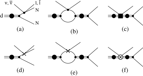
Figure 2: Feynman diagrams for the $\nu d\to lNN$ and $\bar{\nu}d\to\bar{l}NN$ reactions without the Coulomb interaction between two nucleons at LO (a)–(c) and NLO (d)–(f). Vertices with a dot (a cross) interacting with a lepton current are those at LO (NLO) for the single nucleon sector, and those with a filled box (a crossed circle) are vertices at LO (NLO) for the double nucleon sector. See the caption of Fig. 1 as well.

Figure 3: Feynman diagrams for dressed dibaryon propagator for the $pp$ channel. Hatched ovals represent the non-perturbative Coulomb interaction between two protons, which include no interaction diagram and all possible diagrams exchanging a potential photon up to infinite order. See the caption of Fig. 1 as well.

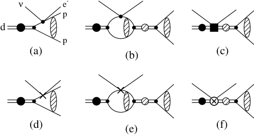
Figure 4: Feynman diagrams for the $\nu d\to e^{-}pp$ reaction at LO (a)–(c) and NLO (d)–(f). See the captions in FIGs. 1, 2, and 3 as well.

II.2 Reaction amplitudes

We write the amplitudes of charged current as

$$A_{qq} = (-1)^{(1+\tau_{q})/2}G^{\prime}_{F}V_{ud}\left[-{\cal A}_{A}^{1S0}+\tilde{\cal A}_{V}^{1S0}-\tilde{\cal A}_{A}^{1S0}+\sum_{J=0}^{2}\left({\cal A}_{V}^{3PJ}-{\cal A}_{A}^{3PJ}\right)\right]\,,$$ (18)

where $q$ denotes neutron ($n$) or proton ($p$), and $\tau_{n(p)}=-1(1)$. Leading order amplitudes are contributed from diagrams (a)-(c) in Figs. 2 and 4, and they are represented in terms of the amplitudes ${\cal A}$ without tilde. Letters $\tilde{\cal A}$ with tilde represent the amplitudes at NLO, and they are from diagrams (d)-(f) in Figs. 2 and 4. The superscripts and subscripts on the amplitudes denote the partial waves and spin states (${}^{1}S_{0}$, ${}^{3}S_{1}$, and ${}^{3}P_{J}$ states) for the final two nucleons and isovector vector ($V$) and axial-vector ($A$) nuclear currents, respectively.

Neutral-current amplitudes are written as

$$A_{np} = \frac{G^{\prime}_{F}}{\sqrt{2}}\left\{(1-2\sin^{2}\theta_{W})\left[\tilde{\cal A}_{V}^{1S0}+\sum_{J=0}^{2}{\cal A}_{V}^{3PJ}\right]\right.$$ (19)

$$\left.-\left({\cal A}_{A}^{1S0}+\tilde{\cal A}_{A}^{1S0}+\sum_{J=0}^{2}{\cal A}_{A}^{3PJ}\right)-2\sin^{2}\theta_{W}\left[{\cal A}_{VS}^{3S1}+\tilde{\cal A}_{VS}^{3S1}\right]\right\}\,,$$

where the subscript ($VS$) denotes the isoscalar vector part of the nuclear current. Because the partial waves are orthogonal, we can write the squared amplitudes as

$$|A_{qq}|^{2} = G^{\prime 2}_{F}V^{2}_{ud}\left[\left|-{\cal A}_{A}^{1S0}+\tilde{\cal A}_{V}^{1S0}-\tilde{\cal A}_{A}^{1S0}\right|^{2}+\sum^{2}_{J=0}\left|{\cal A}_{V}^{3PJ}-{\cal A}_{A}^{3PJ}\right|^{2}\right],$$ (20)

$$|A_{np}|^{2} = \frac{G^{\prime 2}_{F}}{2}\left\{\left|{\cal A}_{A}^{1S0}+\tilde{\cal A}_{A}^{1S0}-(1-2\sin^{2}\theta_{W})\tilde{\cal A}_{V}^{1S0}\right|^{2}+\left|2\sin^{2}\theta_{W}({\cal A}_{VS}^{3S1}+\tilde{\cal A}_{VS}^{3S1})\right|^{2}\right.$$ (21)

$$+\left.\sum^{2}_{J=0}\left|{\cal A}_{A}^{3PJ}-(1-2\sin^{2}\theta_{W}){\cal A}_{V}^{3PJ}\right|^{2}\right\}.$$

Amplitudes for S-wave states can be written as

$${\cal A}_{A}^{1S0} = \vec{\epsilon}_{(l)}\cdot\vec{\epsilon}_{(d)}X_{A}^{1S0}\,,$$ (22)

$$\tilde{\cal A}_{A}^{1S0} = v\cdot\epsilon_{(l)}\hat{q}\cdot\vec{\epsilon}_{(d)}\tilde{X}_{A}^{1S0}\,,$$ (23)

$$\tilde{\cal A}_{V}^{1S0} = i\hat{q}\cdot\left(\vec{\epsilon}_{(d)}\times\vec{\epsilon}_{(l)}\right)\tilde{X}_{V}^{1S0}\,,$$ (24)

$${\cal A}_{VS}^{3S1} = v\cdot\epsilon_{(l)}\vec{\epsilon}^{*}\cdot\vec{\epsilon}_{(d)}X_{VS}^{3S1}\,,$$ (25)

$$\tilde{\cal A}_{VS}^{3S1} = \hat{q}\cdot\vec{\epsilon}_{(l)}\vec{\epsilon}^{*}\cdot\vec{\epsilon}_{(d)}\tilde{X}_{VS}^{3S1}\,,$$ (26)

where $\vec{\epsilon}_{(d)}$ and $\vec{\epsilon}^{*}$ are spin polarization vectors of the incoming deuteron and the final two nucleon ${}^{3}S_{1}$ states, respectively, and $\epsilon^{(l)}_{\mu}$ are the lepton currents. In addition, $\hat{q}=\vec{q}/|\vec{q}|$, where $\vec{q}$ is the momentum transfer between the lepton current and the nuclear current: $\vec{q}=\vec{k}^{\prime}-\vec{k}$. $X$ and $\tilde{X}$ denote the LO and NLO contributions, respectively, and are given by

$$X_{A}^{1S0} = 2g_{A}\sqrt{\frac{2\pi\gamma}{1-\gamma\rho_{d}}}\left\{\frac{}{}\Gamma_{4(1)}^{(NN)}(p,q)\right.$$ (27)

$$\left.+\Gamma_{3(0)}^{(NN)}(p)D_{s}^{(NN)}(p)\left[\Gamma_{3(1)}^{(NN)}(p,q)-\frac{1}{4}(r^{(NN)}_{0}+\rho_{d})+\frac{l_{1A}}{2g_{A}m_{N}}\right]\right\}\,,$$

$$\tilde{X}_{A}^{1S0} = \frac{2g_{A}}{m_{N}}\sqrt{\frac{2\pi\gamma}{1-\gamma\rho_{d}}}\left\{\frac{}{}p\Gamma_{4(2)}^{(NN)}(p,q)\right.$$ (28)

$$\left.+\Gamma_{3(0)}^{(NN)}(p)D_{s}^{(NN)}(p)q\left[\Gamma_{3(2)}^{(NN)}(p,q)-\frac{1}{16}(r^{(NN)}_{0}+\rho_{d})+\frac{l_{2A}}{4g_{A}}\right]\right\}\,,$$

$$\tilde{X}_{V}^{1S0} = -\frac{\mu_{V}q}{m_{N}}\sqrt{\frac{2\pi\gamma}{1-\gamma\rho_{d}}}\left\{\frac{}{}\Gamma_{4(1)}^{(NN)}(p,q)\right.$$ (29)

$$\left.+\Gamma_{3(0)}^{(NN)}(p)D_{s}^{(NN)}(p)\left[\Gamma_{3(1)}^{(NN)}(p,q)-\frac{1}{4}(r^{(NN)}_{0}+\rho_{d})+\frac{l_{1}}{\mu_{V}}\right]\right\}\,,$$

$$X_{VS}^{3S1} = -2\sqrt{\frac{2\pi\gamma}{1-\gamma\rho_{d}}}\left\{\frac{}{}\Gamma_{4(1)}^{(np)}(p,q)+\Gamma_{3(0)}^{(np)}(p)D_{t}^{(np)}(p)\left[\Gamma_{3(1)}^{(np)}(p,q)-\frac{1}{2}\rho_{d}\right]\right\}\,,$$ (30)

$$\tilde{X}_{VS}^{3S1} = -\frac{2}{m_{N}}\sqrt{\frac{2\pi\gamma}{1-\gamma\rho_{d}}}\left\{p\Gamma_{4(2)}^{(np)}(p,q)+\Gamma_{3(0)}^{(np)}(p)D_{t}^{(np)}(p)q\left[\Gamma_{3(2)}^{(np)}(p,q)-\frac{1}{8}\rho_{d}\right]\right\}\,,$$ (31)

where $\gamma$ is the deuteron binding momentum, $\gamma=\sqrt{2m_{N}B}$; $B$ is the deuteron binding energy, and $\mu_{V}=1+\kappa_{V}$. The LECs $l_{1A}$, $l_{2A}$, and $l_{1}$ for the contact interactions are defined as

$$l_{1A} = L_{1A}+\frac{1}{2}m_{N}g_{A}(\rho_{d}+r^{(NN)}_{0})\,,$$ (32)

$$l_{2A} = L_{2A}+\frac{1}{4}g_{A}(\rho_{d}+r^{(NN)}_{0})\,,$$ (33)

$$l_{1} = L_{1}+\frac{1}{4}\mu_{V}(\rho_{d}+r^{(NN)}_{0})\,.$$ (34)

As discussed in Ref. prc2005 , we separate the LECs $L_{1A}$, $L_{2A}$, and $L_{1}$ into two parts: one consists of the effective range terms so as to reproduce the result from the effective range theory, and the other consists of the unfixed constants $l_{1A}$, $l_{2A}$, and $l_{1}$, which may correspond to small corrections from a mechanism at high energy such as meson exchange currents. We note that LECs do not appear for the isoscalar vector parts in Eqs. (30) and (31) due to conserved vector current (CVC). In addition, the sign for $l_{1A}$ above is opposite to that in Refs. plb2008 ; nnfusion .

$\Gamma_{4(1,2)}^{(NN)}(p,q)$ are four-point vertex functions for the $NN=np,nn,pp$ channels, $\Gamma_{3(0)}^{(NN)}(p)$ and $\Gamma_{3(1,2)}^{(NN)}(p,q)$ are three-point vertex functions, and $D_{s}^{(NN)}(p)$ and $D_{t}^{(np)}(p)$ are dressed two-nucleon propagators for spin singlet and spin triplet channels, respectively. For the $np$ and $nn$ channels we have

$$\Gamma_{4(1)}^{(np,nn)}(p,q) = \frac{1}{2pq}\ln\left(\frac{\gamma^{2}+(p+\frac{1}{2}q)^{2}}{\gamma^{2}+(p-\frac{1}{2}q)^{2}}\right)\,,$$ (35)

$$\Gamma_{4(2)}^{(np,nn)}(p,q) = \frac{1}{pq}\left[1-\frac{\gamma^{2}+p^{2}+\frac{1}{4}q^{2}}{2pq}\ln\left(\frac{\gamma^{2}+(p+\frac{1}{2}q)^{2}}{\gamma^{2}+(p-\frac{1}{2}q)^{2}}\right)\right]\,,$$ (36)

$$\Gamma_{3(1)}^{(np,nn)}(p,q) = \frac{1}{q}\left[\frac{\pi}{2}-\arcsin\left(\frac{\gamma^{2}+p^{2}-\frac{1}{4}q^{2}}{\sqrt{(\gamma^{2}+p^{2}+\frac{1}{4}q^{2})^{2}-(pq)^{2}}}\right)+\frac{i}{2}\ln\left(\frac{\gamma^{2}+(p+\frac{1}{2}q)^{2}}{\gamma^{2}+(p-\frac{1}{2}q)^{2}}\right)\right]\,,$$

$$\Gamma_{3(2)}^{(np,nn)}(p,q) = -\frac{\gamma^{2}+p^{2}+\frac{1}{4}q^{2}}{q^{3}}\left[\frac{\pi}{2}-\arcsin\left(\frac{\gamma^{2}+p^{2}-\frac{1}{4}q^{2}}{\sqrt{(\gamma^{2}+p^{2}+\frac{1}{4}q^{2})^{2}-(pq)^{2}}}\right)\right.$$ (38)

$$\left.+\frac{i}{2}\ln\left(\frac{\gamma^{2}+(p+\frac{1}{2}q)^{2}}{\gamma^{2}+(p-\frac{1}{2}q)^{2}}\right)\right]+\frac{1}{q^{2}}(\gamma+ip)\,,$$

$$D_{s}^{(np,nn)}(p) = \frac{1}{-\frac{1}{a_{0}^{(np,nn)}}+\frac{1}{2}r_{0}^{(np,nn)}p^{2}-ip}\,,$$ (39)

$$D_{t}^{(np)}(p) = \frac{1}{-\gamma+\frac{1}{2}\rho_{d}(\gamma^{2}+p^{2})-ip}\,,\ \ \ \Gamma_{3(0)}^{(np,nn)}(p)=1\,,$$ (40)

where $a_{0}^{(NN)}$ are scattering lengths of the $NN$ scattering in the ${}^{1}S_{0}$ channel.

For the $pp$ channel, we include the contribution from the nonperturbative Coulomb interaction in the amplitudes; we follow the calculation method suggested by Ryberg et al. rfhpprc2014 , in which Coulomb Green’s functions are represented in the coordinate space satisfying appropriate boundary conditions. Thus we have

$$\Gamma_{4(1)}^{(pp)}(p,q) = \frac{e^{i\sigma_{0}}}{p}\int_{0}^{\infty}drF_{0}(\eta,pr)j_{0}(\frac{1}{2}qr)e^{-\gamma r}\,,$$ (41)

$$\Gamma_{4(2)}^{(pp)}(p,q) = -e^{i\sigma_{0}}\frac{q}{p^{2}}\left[\frac{1}{2}\int_{0}^{\infty}drF_{0}(\eta,pr)j_{0}(\frac{1}{2}qr)e^{-\gamma r}\right.$$ (42)

$$\left.-\frac{1}{q}\int_{0}^{\infty}drF_{0}(\eta,pr)j_{1}(\frac{1}{2}qr)\left(\frac{1}{r}+\gamma\right)e^{-\gamma r}\right]\,,$$

$$\Gamma_{3(1)}^{(pp)}(p,q) = C_{\eta}\int_{0}^{\infty}drH_{0}^{+}(\eta,pr)j_{0}(\frac{1}{2}qr)e^{-\gamma r}\,,$$ (43)

$$\Gamma_{3(2)}^{(pp)}(p,q) = -C_{\eta}\left[\frac{1}{2}\int_{0}^{\infty}drH_{0}^{+}(\eta,pr)j_{0}(\frac{1}{2}qr)e^{-\gamma r}\right.$$ (44)

$$\left.-\frac{1}{q}\int_{0}^{\infty}drH_{0}^{+}(\eta,pr)j_{1}(\frac{1}{2}qr)\left(\frac{1}{r}+\gamma\right)e^{-\gamma r}\right]\,,$$

$$D_{s}^{(pp)}(p) = \frac{1}{-\frac{1}{a_{0}^{(pp)}}+\frac{1}{2}r_{0}^{(pp)}p^{2}+2\kappa H(\eta)}\,,\ \ \ \Gamma_{3(0)}^{(pp)}(p)=e^{i\sigma_{0}}C_{\eta}\,,$$ (45)

$$H(\eta) = \psi(i\eta)+\frac{1}{2i\eta}-\ln(i\eta)\,,\ \ \ C_{\eta}=\sqrt{\frac{2\pi\eta}{e^{2\pi\eta}-1}}\,,\ \ \ e^{i\sigma_{0}}=\sqrt{\frac{\Gamma(1+i\eta)}{\Gamma(1-i\eta)}}\,,$$ (46)

where $H_{l}^{+}(\eta,\rho)=G_{l}(\eta,\rho)+iF_{l}(\eta,\rho)$; $F_{l}(\eta,\rho)$ and $G_{l}(\eta,\rho)$ are regular and irregular Coulomb wave functions, respectively, and $j_{l}(x)$ are the spherical Bessel functions. $\psi(z)$ is the digamma function with $\eta=\kappa/p$; $\kappa=\alpha_{E}m_{p}/2$ where $\alpha_{E}$ is the fine-structure constant. The $r$-space integrations above can be carried out analytically. The derivation and expression of those integrals are presented in Appendix A.

In a similar manner we write the amplitudes in the $P$-wave states as

$${\cal A}_{V}^{3P0} = v\cdot\epsilon_{(l)}\hat{q}\cdot\vec{\epsilon}_{(d)}X_{V}^{3P0}\,,$$ (47)

$${\cal A}_{A}^{3P0} = i\hat{q}\cdot\left(\vec{\epsilon}_{(l)}\times\vec{\epsilon}_{(d)}\right)X_{A}^{3P0}\,,$$ (48)

$${\cal A}_{V}^{3P1} = iv\cdot\epsilon_{(l)}\vec{\epsilon}^{*}\cdot\left(\hat{q}\times\vec{\epsilon}_{(d)}\right)X_{V}^{3P1}\,,$$ (49)

$${\cal A}_{A}^{3P1} = \left(\vec{\epsilon}^{*}\cdot\vec{\epsilon}_{(l)}\hat{q}\cdot\vec{\epsilon}_{(d)}-\vec{\epsilon}^{*}\cdot\vec{\epsilon}_{(d)}\hat{q}\cdot\vec{\epsilon}_{(l)}\right)X_{A}^{3P1}\,,$$ (50)

$${\cal A}_{V}^{3P2} = v\cdot\epsilon_{(l)}\epsilon^{ij*}\hat{q}^{i}\epsilon_{(d)}^{j}X_{V}^{3P2}\,,$$ (51)

$${\cal A}_{A}^{3P2} = i\epsilon^{ij*}\hat{q}^{i}\epsilon^{jkl}\epsilon_{(l)}^{k}\epsilon_{(d)}^{l}X_{A}^{3P2}\,,$$ (52)

with

$$X_{V}^{3P0} = -2\sqrt{\frac{2\pi\gamma}{1-\gamma\rho_{d}}}\Gamma_{4(3)}^{(NN)}(p,q)\,,$$ (53)

$$X^{3P1}_{V} = \sqrt{\frac{3}{2}}X_{V}^{3P0}\,,\ \ \ X^{3P2}_{V}=\sqrt{3}X_{V}^{3P0}\,,$$ (54)

$$X^{3PJ}_{A} = -g_{A}X^{3PJ}_{V}\,,$$ (55)

where $J=0,1,2$, and $\epsilon_{i}^{*}$ and $\epsilon_{ij}^{*}$ are a vector and a symmetric tensor representing the final two nucleons for $J=1$ and 2 states, respectively. For the $np$ and $nn$ channels, $\Gamma_{4(3)}^{(np,nn)}(p,q)=\Gamma_{4(2)}^{(np,nn)}(p,q)$, and for the $pp$ channel we have

$$\Gamma_{4(3)}^{(pp)}(p,q) = -\frac{e^{i\sigma_{1}}}{p}\int_{0}^{\infty}drF_{1}(\eta,pr)j_{1}(\frac{1}{2}qr)e^{-\gamma r}\,,$$ (56)

with

$$e^{i\sigma_{1}}=\sqrt{\frac{\Gamma(2+i\eta)}{\Gamma(2-i\eta)}}\,.$$ (57)

An analytic expression of the vertex function $\Gamma_{4(3)}^{(pp)}(p,q)$ is presented in Appendix A as well.

Summing over spins in the initial and final states, we obtain the result

$$\sum_{\rm spins}|A_{qq}|^{2}=8G_{F}^{\prime 2}V^{2}_{ud}\left\{(3E^{\prime}E-\vec{k}^{\prime}\cdot\vec{k})\left|X_{A}^{1S0}\right|^{2}\right.-\left(E^{\prime}\hat{q}\cdot\vec{k}+E\hat{q}\cdot\vec{k}^{\prime}\right)\left[X_{A}^{1S0*}\tilde{X}_{A}^{1S0}+\tilde{X}_{A}^{1S0*}X_{A}^{1S0}\right]$$

$$\mp 2\left(E^{\prime}\hat{q}\cdot\vec{k}-E\hat{q}\cdot\vec{k}^{\prime}\right)\left[X_{A}^{1S0*}\tilde{X}_{V}^{1S0}+\tilde{X}_{V}^{1S0*}X_{A}^{1S0}\right]$$

$$+(E^{\prime}E+\vec{k}^{\prime}\cdot\vec{k})\left|\tilde{X}_{A}^{1S0}\right|^{2}+2(E^{\prime}E-\hat{q}\cdot\vec{k}^{\prime}\hat{q}\cdot\vec{k})\left|\tilde{X}_{V}^{1S0}\right|^{2}$$

$$+(E^{\prime}E+\vec{k}^{\prime}\cdot\vec{k})\left[\left|X_{V}^{3P0}\right|^{2}+2\left|X_{V}^{3P1}\right|^{2}+\frac{5}{3}\left|X_{V}^{3P2}\right|^{2}\right]$$

$$+2(E^{\prime}E-\hat{q}\cdot\vec{k}^{\prime}\hat{q}\cdot\vec{k})\left|X_{A}^{3P0}\right|^{2}+2(2E^{\prime}E-2\vec{k}^{\prime}\cdot\vec{k}-\hat{q}\cdot\vec{k}^{\prime}\hat{q}\cdot\vec{k})\left|X_{A}^{3P1}\right|^{2}$$

$$\left.+4(20E^{\prime}E-6\vec{k}^{\prime}\cdot\vec{k}+2\hat{q}\cdot\vec{k}^{\prime}\hat{q}\cdot\vec{k})\left|X_{A}^{3P2}\right|^{2}\right\}\,,$$ (58)

$$\sum_{\rm spins}|A_{np}|^{2}=4G_{F}^{\prime 2}\left\{(3E^{\prime}E-\vec{k}^{\prime}\cdot\vec{k})\left|X_{A}^{1S0}\right|^{2}-\left(E^{\prime}\hat{q}\cdot\vec{k}+E\hat{q}\cdot\vec{k}^{\prime}\right)\left[X_{A}^{1S0*}\tilde{X}_{A}^{1S0}+\tilde{X}_{A}^{1S0*}X_{A}^{1S0}\right]\right.$$

$$\mp 2\left(E^{\prime}\hat{q}\cdot\vec{k}-E\hat{q}\cdot\vec{k}^{\prime}\right)\left(1-2\sin^{2}\theta_{W}\right)\left[X_{A}^{1S0*}\tilde{X}_{V}^{1S0}+\tilde{X}_{V}^{1S0*}X_{A}^{1S0}\right]+(E^{\prime}E+\vec{k}^{\prime}\cdot\vec{k})\left|\tilde{X}_{A}^{1S0}\right|^{2}$$

$$+2(E^{\prime}E-\hat{q}\cdot\vec{k}^{\prime}\hat{q}\cdot\vec{k})\left(1-2\sin^{2}\theta_{W}\right)^{2}\left|\tilde{X}_{V}^{1S0}\right|^{2}+12\sin^{4}\theta_{W}(E^{\prime}E+\vec{k}^{\prime}\cdot\vec{k})\left|X_{VS}^{3S1}\right|^{2}$$

$$-12\sin^{4}\theta_{W}\left(E^{\prime}\hat{q}\cdot\vec{k}+E\hat{q}\cdot\vec{k}^{\prime}\right)\left[X_{VS}^{3S1*}\tilde{X}_{VS}^{3S1}+\tilde{X}_{VS}^{3S1*}X_{VS}^{3S1}\right]$$

$$+12\sin^{4}\theta_{W}\left(E^{\prime}E-\vec{k}^{\prime}\cdot\vec{k}-2\hat{q}\cdot\vec{k}^{\prime}\hat{q}\cdot\vec{k}\right)\left|\tilde{X}_{VS}^{3S1}\right|^{2}$$

$$+(E^{\prime}E+\vec{k}^{\prime}\cdot\vec{k})\left(1-2\sin^{2}\theta_{W}\right)^{2}\left[\left|X_{V}^{3P0}\right|^{2}+2\left|X_{V}^{3P1}\right|^{2}+\frac{5}{3}\left|X_{V}^{3P2}\right|^{2}\right]$$

$$+2(E^{\prime}E-\hat{q}\cdot\vec{k}^{\prime}\hat{q}\cdot\vec{k})\left|X_{A}^{3P0}\right|^{2}+2(2E^{\prime}E-2\vec{k}^{\prime}\cdot\vec{k}-\hat{q}\cdot\vec{k}^{\prime}\hat{q}\cdot\vec{k})\left|X_{A}^{3P1}\right|^{2}$$

$$\left.+4(20E^{\prime}E-6\vec{k}^{\prime}\cdot\vec{k}+2\hat{q}\cdot\vec{k}^{\prime}\hat{q}\cdot\vec{k})\left|X_{A}^{3P2}\right|^{2}\right\}\,,$$ (59)

where we have used the spin summation relations presented in Appendix B.

III Numerical results

First we specify the values of LECs. Low-energy constant $l_{1}$ is fitted to the total cross section of the radiative neutron-proton capture process at threshold prc2005 . Data that can constrain the numerical value of $l_{1A}$ directly from experiment are not available; we employ two values of $l_{1A}$ reported in the previous works plb2008 ; nnfusion . In the work on proton-proton fusion plb2008 , $l_{1A}$ is determined by using a ratio of the two-body amplitude to the one-body one for $pp$ fusion (reported in Eq. (28) of Ref. petal-prc03 ) calculated in the hybrid EFT approach, where the strength of the two-body operator is constrained by the tritium lifetime; it gives $l_{1A}=0.50\pm 0.03$. Another way to fix $l_{1A}$ is proposed in the work on neutron-neutron fusion nnfusion , in which a value of $l_{1A}$ is constrained by the cross section of the $\nu d$ reaction for the $\nu d\to e^{+}nn$ channel reported in Refs. netal-npa ; hybrid ; it gives $l_{1A}=0.33\pm 0.03$. Since a robust way to fix the value of $l_{1A}$ is absent at present, $l_{1A}$ is a source of uncertainty in the theoretical prediction. Without any priority to a specific value, we use both values $l_{1A}=0.33$ and $0.50$ in the calculation of the total cross sections.  The Lagrangian term proportional to LEC $l_{2A}$ has a derivative one order higher than the terms proportional to $l_{1}$ and $l_{1A}$. Since the perturbative expansion is performed with respect to either energy or momentum of the particles, higher order derivatives will be suppressed compared to the lower order ones. In addition, since experimental data that can constrain $l_{2A}$ are not available, we assume $l_{2A}=0$ for simplicity.  Scattering lengths $a^{(NN)}_{0}$ are taking the values $-23.73$ fm, $-18.50$ fm and $-7.82$ fm for $np$, $nn$ and $pp$ states, respectively, and effective ranges $r^{(NN)}_{0}$ are 2.73 fm, 2.83 fm and 2.78 fm for the $np$, $nn$, and $pp$ states, respectively.

$E_{\nu}$	$\nu np$	$\bar{\nu}np$	$e^{+}nn$	$e^{-}pp$
2	0	0	0	0.003665
3	0.003366	0.003330	0	0.04706
4	0.03070	0.03021	0	0.1567
5	0.09495	0.09291	0.02841	0.3459
6	0.2017	0.1962	0.1192	0.6230
7	0.3540	0.3425	0.2823	0.9936
8	0.5540	0.5329	0.5225	1.462
9	0.8029	0.7679	0.8422	2.032
10	1.102	1.048	1.242	2.705
11	1.452	1.373	1.722	3.485
12	1.853	1.742	2.282	4.374
13	2.307	2.157	2.922	5.374
14	2.813	2.616	3.640	6.488
15	3.373	3.119	4.436	7.716
16	3.987	3.667	5.309	9.062
17	4.656	4.259	6.259	10.53
18	5.380	4.895	7.285	12.12
19	6.161	5.576	8.386	13.83
20	6.998	6.301	9.563	15.67

Table 1: Total cross sections of neutrino-deuteron scattering as functions of the incident neutrino energy. Reaction types are denoted by the particles in the final states. Incident neutrino energy $E_{\nu}$ is in MeV, and the total cross sections are in units of $10^{-42}{\rm cm}^{2}$.

Table 1 shows the total cross sections in units of $10^{-42}$ cm². For the $np$ and $pp$ final states, results with $l_{1A}=0.50$ are presented, and the results for the $nn$ state are with $l_{1A}=0.33$. The general trend is a monotonic increase with energy, and the rate is larger in charged-current processes than in neutral ones. For a better overall view, results in Table 1 are plotted in Fig. 5. As a benchmark for comparison with other theories, we include the result of Ref. snpa , which is labeled SNPA meaning standard nuclear physics approach. In the SNPA, initial- and final-state wave functions are the solutions of Schrödinger equations with modern phenomenological $NN$ potentials, and transition operators consist of one-body impulse approximation and two-body meson-exchange currents. In our work we use partial wave expansion of the final state up to $P$-wave, but the SNPA results include states up to $J=6$. Despite the huge differences in the basic formalism of the two theories on one hand, and partial waves in the final state on the other hand, predictions of the two works agree remarkably well. Recent EFT works butler ; baroni show agreement with SNPA within the order of 1%. A refined comparison is in order next.

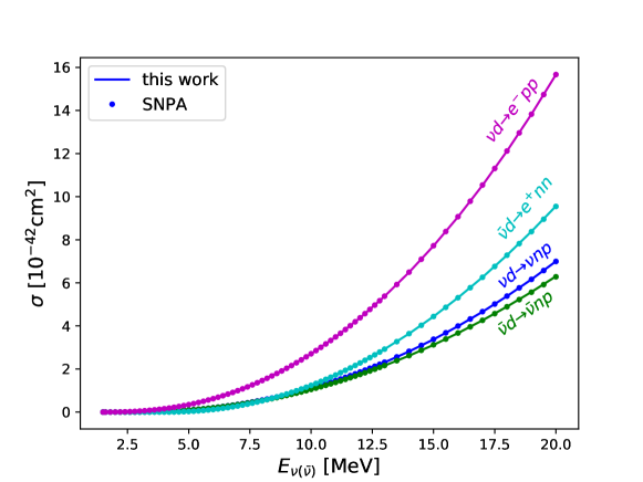
xxx

Figure 5: Color online. Total cross sections (cm²) as functions of the incident neutrino energy $E_{\nu}$. Solid lines denote the result of this work for $\nu np$ (blue), $\bar{\nu}np$ (green), $e^{+}nn$ (cyan) and $e^{-}pp$ (magenta). Dots present the result of SNPA snpa .

$E_{\nu}$	$\nu np$		$\bar{\nu}np$		$e^{+}nn$		$e^{-}pp$
$l_{1A}$	x 0.33	xx 0.50	x 0.33	xx 0.50	x0.33	xx 0.50	x 0.33	xx 0.50
2	-	-	-	-	-	-	$-0.77$	$-0.13$
3	$-1.79$	$-1.06$	$-1.81$	$-1.07$	-	-	$-0.82$	$-0.12$
4	$-1.69$	$-0.94$	$-1.69$	$-0.92$	-	-	$-0.88$	$-0.13$
5	$-1.60$	$-0.78$	$-1.61$	$-0.78$	0.46	0.92	$-0.89$	$-0.11$
6	$-1.53$	$-0.69$	$-1.54$	$-0.71$	0.18	1.01	$-0.90$	$-0.10$
7	$-1.47$	$-0.62$	$-1.78$	$-0.61$	0.10	0.92	$-0.92$	$-0.10$
8	$-1.44$	$-0.56$	$-1.44$	$-0.54$	0.10	0.96	$-0.97$	$-0.13$
9	$-1.40$	$-0.51$	$-1.40$	$-0.51$	0.07	0.94	$-0.96$	$-0.12$
10	$-1.37$	$-0.47$	$-1.42$	$-0.48$	0.01	0.90	$-0.96$	$-0.10$
11	$-1.36$	$-0.44$	$-1.33$	$-0.38$	0.02	0.93	$-0.98$	$-0.11$
12	$-1.31$	$-0.38$	$-1.28$	$-0.31$	0.02	0.95	$-0.99$	$-0.11$
13	$-1.26$	$-0.32$	$-1.26$	$-0.28$	$-0.00$	0.94	$-1.00$	$-0.11$
14	$-1.26$	$-0.31$	$-1.22$	$-0.23$	$-0.02$	0.94	$-1.01$	$-0.11$
15	$-1.22$	$-0.26$	$-1.18$	$-0.18$	$-0.02$	0.95	$-1.01$	$-0.10$
16	$-1.16$	$-0.20$	$-1.12$	$-0.11$	$-0.01$	0.97	$-1.01$	$-0.10$
17	$-1.12$	$-0.15$	$-1.04$	$-0.02$	0.02	1.01	$-1.03$	$-0.11$
18	$-1.06$	$-0.09$	$-0.94$	$0.09$	0.04	1.04	$-0.95$	$-0.03$
19	$-1.00$	$-0.02$	$-0.84$	$0.20$	0.09	1.11	$-0.93$	$-0.01$
20	$-0.93$	$0.06$	$-0.72$	$0.32$	0.16	1.19	$-0.94$	$-0.01$

Table 2: Differences of between our result and those using SNPA. Difference is calculated in % as (this work $-$ other)/other$\times 100$.

In Table 2, we show the difference between our work and SNPA. For each reaction channel, we calculate the differences with both $l_{1A}=0.33$ and $0.50$. From the resulting differences, one can deduce that the total cross is larger with $l_{1A}=0.50$ than with 0.33 for all reactions and energies. $l_{1A}=0.50$ is adopted from the work on $pp$ fusion, and it gives better agreement with SNPA than $l_{1A}=0.33$ for the $e^{-}pp$ reaction channel. On the other hand, the total cross section of the $e^{+}nn$ channel is closer to SNPA with $l_{1A}=0.33$ than 0.50. It turns out that $l_{1A}=0.50$ gives better agreement with SNPA than 0.33 for the neutral-current processes. The gap between the differences of $l_{1A}=0.33$ and 0.50 is in the interval 0.7$-$1.1%, and it is weakly dependent on the reaction type and energy. We take this as a theoretical uncertainty in this work originating from the LEC $l_{1A}$. There are other sources of uncertainties such as truncation at NLO in the perturbative expansion and $P$-wave approximation in the partial wave expansion. Discussions of these uncertainties will be presented in the following paragraphs.

	LO/total			S-wave/total			S-wave/EFT*
$E_{\nu}$	$\nu np$	$e^{-}pp$		$\nu np$	$e^{-}pp$		$\nu np$	$e^{-}pp$
5	0.9886	0.9777		0.9999	0.9997		-	-
10	0.9745	0.9525		0.9975	0.9963		0.994	0.999
15	0.9609	0.9288		0.9902	0.9875		0.997	1.003
20	0.9482	0.9070		0.9764	0.9723		1.000	1.007

Table 3: Ratios of the LO contribution to the total (LO/total), S-wave contribution to the total (S-wave/total), and S-wave contribution in our work to that in EFT* hybrid (S-wave/EFT*).

The relative contribution of LO amplitudes to the total cross section is shown in the column ‘LO/total’ for the $\nu np$ and $e^{-}pp$ reactions in Table 3. At energies close to threshold, LO takes 98$-$99% of the total. Its portion decreases monotonically as energy increases, and it reaches $91-95$% at 20 MeV. This result satisfies the general behavior of perturbation theory: (i) lower orders dominate at low energies, (ii) contributions of higher orders increase as the energy increases, and (iii) higher order contributions should be sufficiently smaller than those of lower orders in the considered energy range.

In order to check the validity of partial wave approximation in the final state, we consider the contribution of $S$-wave states. The column ‘$S$-wave/total’ in Table 3 shows the ratio of cross section from the $S$-wave contribution to that of the full contribution. In the solar neutrino energy region, the total result is absolutely dominated by the $S$ waves. However, though it is small, the contribution of higher partial waves increases with energy. In our result the contribution of P waves at $E_{\nu}=5$ MeV is 0.03% at most, and it increases to 2$-$3% at $E_{\nu}=20$ MeV. In the work using SNPA snpa , the authors performed a similar analysis of the $S$-wave contribution. At $E_{\nu}=20$ MeV, the proportions of the ${}^{1}{\rm S}_{0}$ state to the net value are obtained as 0.972 and 0.964 for $\nu np$ and $e^{-}pp$ reactions, respectively. These values are smaller than our results only by 0.004 and 0.008, so the two very different models give consistent predictions about the role of S-wave states in the final state. The $P$-wave contribution was also calculated separately in snpa . At $E_{\nu}=20$ MeV, the sum of $S$- and $P$-wave contribution is 99.9% of the total result which includes the partial waves to $J=6$. Therefore contributions from partial waves higher than the $D$ state will not be a source of uncertainty at the order of 1% for the solar neutrino energies.

In Ref. hybrid , the authors investigated the same problem with a pionful EFT. In that work, final state wave functions contain only the $S$-wave states. In the column denoted ‘S-wave/EFT*’ in Table 3, we present the ratio of $S$-wave contributions in our work to those of EFT*. The two theories agree in the range 0.994$-$1.007, so in practice the two theories predict equivalent results for the total cross section.

IV Summary

We considered the breakup of deuterons by neutrinos and antineutrinos at solar neutrino energies. We calculated the total cross section of the neutral-current reactions $\nu d\to\nu np$, $\bar{\nu}d\to\bar{\nu}np$, and the charged-current ones $\bar{\nu}d\to e^{+}nn$, $\nu d\to e^{-}pp$ in the framework of a pionless effective field theory with dibaryon fields up to the next-to-leading order. We included the Coulomb interaction between two protons nonperturbatively while analytic expressions of the amplitudes were obtained. We estimated the uncertainty of our theory by comparing our result to those obtained from various theories and models.

In the comparison to the work that employs phenomenological nucleon-nucleon potential models, the contribution of the $S$-wave state in the final state agrees well with the result of snpa , and it is confirmed that the truncation at $P$ waves in the final state wave functions is a good approximation. The main source of the uncertainty was identified as a low-energy constant $l_{1A}$ which determines the strength of the axial four-nucleon contact interactions. The low-energy constant determined from available experimental data gives uncertainties about 1% or less.

We compared our results of the $S$-wave contribution with those obtained from a pionful effective field theory in which expansion is performed up to next-to-next-to-next-to-leading order hybrid . We found that the two theories predict practically identical results, with a difference of about 0.7% at most.

Convergence of the theory was checked by isolating the leading order contribution from the total. At low energies, leading order contributes almost 100% of the total, and its portion decreases as the energy increases. For the $\nu np$ reaction, leading order takes 95% of the total at $E_{\nu}=20$ MeV. This ratio of the S-wave contribution is similar to the ratio of next-to-next-to-leading order to leading order obtained in a pionless effective field theory butler . This comparison demonstrates that the rate of convergence could be improved by the introduction of dibaryon fields.

Our result underestimates the result of a benchmark calculation snpa by about 1%. On the other hand, another pionless effective field theory butler gives a result very similar to snpa , and a chiral perturbation theory baroni obtains results larger than snpa by about 1%. Therefore one can conclude that the uncertainty one can obtain from the state-of-the-art theories is about 2$-$3% in the solar neutrino energy range. Precise determination of LECs from experiment will be important to reduce the theoretical uncertainty.

Appendix A

Analytic expression of the four-point vertex functions $\Gamma_{4(1)}^{(pp)}(p,q)$ and $\Gamma_{4(3)}^{(pp)}(p,q)$ are calculated by using formula NISTHB ,

$$F_{l}(\eta,\rho) = C_{l}(\eta)\rho^{l+1}e^{\mp i\rho}M(l+1\mp i\eta,2l+2,\pm 2i\rho)\,,$$ (60)

where $M(a,b,z)$ is the Kummer function and

$$C_{l}(\eta) = \frac{2^{l}e^{-\frac{\pi}{2}\eta}|\Gamma(l+1+i\eta)|}{(2l+1)!}=\frac{2^{l}}{(2+1)!}\sqrt{\frac{2\pi\eta}{e^{2\pi\eta}-1}\prod_{k=1}^{l}(\eta^{2}+k^{2})}\,.$$ (61)

The expressions for the ($\pm$ or $\mp$) signs in Eq. (60) are identical because of the relation $M(a,b,z)=e^{z}M(b-a,b,-z)$. Using another relation,

$$\int_{0}^{\infty}e^{-zt}t^{b-1}M(a,c,kt)dt = \Gamma(b)z^{-b}{}_{2}F_{1}(a,b,c;k/z)\,,$$ (62)

with Re$[b]>0$, Re$[z]>\textrm{max}(\rm{Re}[k],0)$, where ${}_{2}F_{1}(a,b,c;z)$ is a hypergeometric function, we have

$$\Gamma_{4(1)}^{(pp)}(p,q) = \frac{e^{i\sigma_{0}}}{p}\int_{0}^{\infty}drF_{0}(\eta,pr)j_{0}(\frac{1}{2}qr)e^{-\gamma r}$$ (63)

$$= i\frac{e^{i\sigma_{0}}}{q}C_{\eta}\left[\frac{1}{\gamma+i(p+\frac{1}{2}q)}{}_{2}F_{1}\left(1-i\eta,1,2;\frac{2ip}{\gamma+i(p+\frac{1}{2}q)}\right)\right.$$

$$\left.-\frac{1}{\gamma+i(p-\frac{1}{2}q)}{}_{2}F_{1}\left(1-i\eta,1,2;\frac{2ip}{\gamma+i(p-\frac{1}{2}q)}\right)\right]\,,$$

$$\Gamma_{4(3)}^{(pp)}(p,q) = -\frac{e^{i\sigma_{1}}}{p}\int_{0}^{\infty}drF_{1}(\eta,pr)j_{1}(\frac{1}{2}qr)e^{-\gamma r}$$ (64)

$$= -\frac{1}{3}pe^{i\sigma_{1}}\sqrt{\frac{2\pi\eta(1+\eta^{2})}{e^{2\pi\eta}-1}}$$

$$\times\left\{\frac{2i}{q^{2}}\left[\frac{1}{\gamma+i(p+\frac{1}{2}q)}{}_{2}F_{1}\left(2-i\eta,1,4;\frac{2ip}{\gamma+i(p+\frac{1}{2}q)}\right)\right.\right.$$

$$\left.-\frac{1}{\gamma+i(p-\frac{1}{2}q)}{}_{2}F_{1}\left(2-i\eta,1,4;\frac{2ip}{\gamma+i(p-\frac{1}{2}q)}\right)\right]$$

$$-\frac{1}{q}\left[\frac{1}{[\gamma+i(p+\frac{1}{2}q)]^{2}}{}_{2}F_{1}\left(2-i\eta,2,4;\frac{2ip}{\gamma+i(p+\frac{1}{2}q)}\right)\right.$$

$$\left.\left.+\frac{1}{[\gamma+i(p-\frac{1}{2}q)]^{2}}{}_{2}F_{1}\left(2-i\eta,2,4;\frac{2ip}{\gamma+i(p-\frac{1}{2}q)}\right)\right]\right\}\,.$$

The four point vertex $\Gamma_{4(2)}^{(pp)}(p,q)$ can be represented by using the result for $\Gamma_{4(1)}^{(pp)}(p,q)$ and an integration,

$$I_{3} = \int_{0}^{\infty}drF_{0}(\eta,pr)j_{1}(\frac{1}{2}qr)\left(\frac{1}{r}+\gamma\right)e^{-\gamma r}\,,$$ (65)

and we have

$$I_{3} = pC_{\eta}\sum_{n=1}^{\infty}(-1)^{n}\left[\frac{1}{(2n+1)!}-\frac{1}{(2n)!}\right]\left(\frac{q}{2}\right)^{2n-1}$$ (66)

$$\times\left[\frac{\gamma\Gamma(2n+1)}{(\gamma+ip)^{2n+1}}{}_{2}F_{1}\left(1-i\eta,2n+1,2;\frac{2ip}{\gamma+ip}\right)\right.$$

$$\left.+\frac{\Gamma(2n)}{(\gamma+ip)^{2n}}{}_{2}F_{1}\left(1-i\eta,2n,2;\frac{2ip}{\gamma+ip}\right)\right]\,.$$

An analytic expression for the three-point vertex function $\Gamma_{3(1)}^{(pp)}(p,q)$ is obtained by using formulas,

$$H_{l}^{\pm}(\eta,\rho) = (\mp)^{l}e^{\frac{\pi}{2}\eta\pm i\sigma_{l}}W_{\mp i\eta,l+\frac{1}{2}}(\mp 2i\rho)\,,$$ (67)

$$\int_{0}^{\infty}dte^{-pt}t^{\nu-1}W_{\kappa,\mu}(at) = \frac{\Gamma(\mu+\nu+\frac{1}{2})\Gamma(\nu-\mu+\frac{1}{2})a^{\nu+\frac{1}{2}}}{\Gamma(\nu-\kappa+1)(p+\frac{1}{2}a)^{\mu+\nu+\frac{1}{2}}}$$ (68)

$$\times{}_{2}F_{1}\left(\mu+\nu+\frac{1}{2},\mu-\kappa+\frac{1}{2},\nu-\kappa+1;\frac{p-\frac{1}{2}a}{p+\frac{1}{2}a}\right)\,,$$

with Re$[\nu\pm\mu]>-\frac{1}{2}$ and Re$\left[p+\frac{1}{2}a\right]>0$, and we have

$$\Gamma_{3(1)}^{(pp)}(p,q) = C_{\eta}\int_{0}^{\infty}drH^{+}_{0}(\eta,pr)j_{0}(\frac{1}{2}qr)e^{-\gamma r}$$ (69)

$$= C_{\eta}e^{\frac{\pi}{2}\eta+i\sigma_{0}}(-2ip)\sum_{n=0}^{\infty}\frac{(-1)^{n}}{(\gamma-ip)^{2n+2}}\left(\frac{q}{2}\right)^{2n}\frac{\Gamma(2n+1)}{\Gamma(2n+2+i\eta)}$$

$$\times_{2}F_{1}\left(2n+2,1+i\eta,2n+2+i\eta;\frac{\gamma+ip}{\gamma-ip}\right)\,.$$

The three point vertex function $\Gamma_{3(2)}^{(pp)}(p,q)$ is represented by using the result of $\Gamma_{3(1)}^{(pp)}(p,q)$ and an integral,

$$I_{5} = \int_{0}^{\infty}drH_{0}^{+}(\eta,pr)j_{1}(\frac{1}{2}qr)\left(\frac{1}{r}+\gamma\right)e^{-\gamma r}\,,$$ (70)

and we have

$$I_{5} = -2ipe^{\frac{\pi}{2}\eta+i\sigma_{0}}\sum_{n=1}^{\infty}(-1)^{n}\left[\frac{1}{(2n+1)!}-\frac{1}{(2n)!}\right]\left(\frac{q}{2}\right)^{2n-1}$$ (71)

$$\times\left[\frac{\gamma}{(\gamma-ip)^{2n-1}}\frac{\Gamma(2n+1)\Gamma(2n)}{\Gamma(2n+1+i\eta)}{}_{2}F_{1}\left(2n+1,1+i\eta,2n+1+i\eta;\frac{\gamma+ip}{\gamma-ip}\right)\right.$$

$$\left.+\frac{1}{(\gamma-ip)^{2n}}\frac{\Gamma(2n)\Gamma(2n-1)}{\Gamma(2n+i\eta)}{}_{2}F_{1}\left(2n,1+i\eta,2n+i\eta;\frac{\gamma+ip}{\gamma-ip}\right)\right]\,.$$

Appendix B

Using the spin summation relations,

$$\sum_{spins}\epsilon_{(d)i}\epsilon_{(d)j}^{*} = \delta_{ij}\,,$$ (72)

$$\sum_{spins}\epsilon_{(l)}^{\alpha}\epsilon_{(l)}^{*\beta} = 8\left(k^{\prime\alpha}k^{\beta}+k^{\prime\beta}k^{\alpha}-g^{\alpha\beta}k^{\prime}\cdot k\pm i\epsilon^{\alpha\beta\mu\nu}k^{\prime}_{\mu}k_{\nu}\right)\,,$$ (73)

where the $\pm$ signs correspond to the initial neutrino and the antineutrino states, respectively, we have the spin summation relations for ¹S₀ channel as

$$\sum_{spins}\left|\vec{\epsilon}_{(l)}\cdot\vec{\epsilon}_{(d)}\right|^{2} = 8\left(3E^{\prime}E-\vec{k}^{\prime}\cdot\vec{k}\right)\,,$$ (74)

$$\sum_{spins}\vec{\epsilon}_{(l)}^{*}\cdot\vec{\epsilon}_{(d)}^{*}v\cdot\epsilon_{(l)}\hat{q}\cdot\vec{\epsilon}_{(d)} = -8\left[E^{\prime}\hat{q}\cdot\vec{k}+E\hat{q}\cdot\vec{k}^{\prime}\pm i\hat{q}\cdot\left(\vec{k}^{\prime}\times\vec{k}\right)\right]\,,$$ (75)

$$\sum_{spins}v\cdot\epsilon_{(l)}^{*}\hat{q}\cdot\vec{\epsilon}_{(d)}^{*}\vec{\epsilon}_{(l)}\cdot\vec{\epsilon}_{(d)} = -8\left[E^{\prime}\hat{q}\cdot\vec{k}+E\hat{q}\cdot\vec{k}^{\prime}\mp i\hat{q}\cdot\left(\vec{k}^{\prime}\times\vec{k}\right)\right]\,,$$ (76)

$$-\sum_{spins}\vec{\epsilon}_{(l)}^{*}\cdot\vec{\epsilon}_{(d)}^{*}i\hat{q}\cdot\left(\vec{\epsilon}_{(d)}\times\vec{\epsilon}_{(l)}\right) = \mp 16\left(E^{\prime}\hat{q}\cdot\vec{k}-E\hat{q}\cdot\vec{k}^{\prime}\right)\,,$$ (77)

$$\sum_{spins}i\hat{q}\cdot\left(\vec{\epsilon}_{(d)}^{*}\times\vec{\epsilon}_{(l)}^{*}\right)\vec{\epsilon}_{(l)}\cdot\vec{\epsilon}_{(d)} = \mp 16\left(E^{\prime}\hat{q}\cdot\vec{k}-E\hat{q}\cdot\vec{k}^{\prime}\right)\,,$$ (78)

$$\sum_{spins}\left|v\cdot\epsilon_{(l)}\hat{q}\cdot\vec{\epsilon}_{(d)}\right|^{2} = 8\left(E^{\prime}E+\vec{k}^{\prime}\cdot\vec{k}\right)\,,$$ (79)

$$\sum_{spins}\left|\hat{q}\cdot\left(\vec{\epsilon}_{(d)}\times\vec{\epsilon}_{(l)}\right)\right|^{2} = 16\left(E^{\prime}E-\hat{q}\cdot\vec{k}^{\prime}\hat{q}\cdot\vec{k}\right)\,,$$ (80)

$$\sum_{spins}v\cdot\epsilon_{(l)}^{*}\hat{q}\cdot\vec{\epsilon}_{(d)}^{*}i\hat{q}\cdot\left(\vec{\epsilon}_{(d)}\times\vec{\epsilon}_{(l)}\right) = \sum_{spins}i\hat{q}\cdot\left(\vec{\epsilon}_{(d)}^{*}\times\vec{\epsilon}_{(l)}^{*}\right)v\cdot\epsilon_{(l)}\hat{q}\cdot\vec{\epsilon}_{(d)}=0\,.$$ (81)

For the ³S₁ channel, we have

$$\sum_{spins}\left|v\cdot\epsilon_{(l)}\vec{\epsilon}^{*}\cdot\vec{\epsilon}_{(d)}\right|^{2} = 24\left(E^{\prime}E+\vec{k}^{\prime}\cdot\vec{k}\right)\,,$$ (82)

$$\sum_{spins}v\cdot\epsilon_{(l)}^{*}\vec{\epsilon}\cdot\vec{\epsilon}_{(d)}^{*}\hat{q}\cdot\vec{\epsilon}_{(l)}\vec{\epsilon}^{*}\cdot\vec{\epsilon}_{(d)} = -24\left[E^{\prime}\hat{q}\cdot\vec{k}+E\hat{q}\cdot\vec{k}^{\prime}\mp i\hat{q}\cdot\left(\vec{k}^{\prime}\times\vec{k}\right)\right]\,,$$ (83)

$$\sum_{spins}\hat{q}\cdot\vec{\epsilon}_{(l)}^{*}\vec{\epsilon}\cdot\vec{\epsilon}_{(d)}^{*}v\cdot\epsilon_{(l)}\vec{\epsilon}^{*}\cdot\vec{\epsilon}_{(d)} = -24\left[E^{\prime}\hat{q}\cdot\vec{k}+E\hat{q}\cdot\vec{k}^{\prime}\pm i\hat{q}\cdot\left(\vec{k}^{\prime}\times\vec{k}\right)\right]\,,$$ (84)

$$\sum_{spins}\left|\hat{q}\cdot\vec{\epsilon}_{(l)}\vec{\epsilon}^{*}\cdot\vec{\epsilon}_{(d)}\right|^{2} = 24\left(E^{\prime}E-\vec{k}^{\prime}\cdot\vec{k}-2\hat{q}\cdot\vec{k}^{\prime}\hat{q}\cdot\vec{k}\right)\,.$$ (85)

For the ³P₀ channel, the terms at LO are the same as those for the ¹S₀ channel.

For the ³P₁ channel at LO, using a spin summation relation for the polarization vector $\epsilon_{i}$ for the $J=1$ state,

$$\sum_{spins}\epsilon_{i}\epsilon_{j}^{*}=\delta_{ij}\,,$$ (86)

we have

$$\sum_{spins}\left|iv\cdot\epsilon_{(l)}\vec{\epsilon}^{*}\cdot\left(\hat{q}\times\vec{\epsilon}_{(d)}\right)\right|^{2}=16\left(E^{\prime}E+\vec{k}^{\prime}\cdot\vec{k}\right)\,,$$ (88)

$$\sum_{spins}\left|\vec{\epsilon}^{*}\cdot\vec{\epsilon}_{(l)}\hat{q}\cdot\vec{\epsilon}_{(d)}-\vec{\epsilon}^{*}\cdot\vec{\epsilon}_{(d)}\hat{q}\cdot\vec{\epsilon}_{(l)}\right|^{2}=16\left(2E^{\prime}E-2\vec{k}^{\prime}\cdot\vec{k}-\hat{q}\cdot\vec{k}^{\prime}\hat{q}\cdot\vec{k}\right)\,,$$

$$\sum_{spins}iv\cdot\epsilon_{(l)}\vec{\epsilon}^{*}\cdot\left(\hat{q}\times\vec{\epsilon}_{(d)}\right)\left(\vec{\epsilon}\cdot\vec{\epsilon}_{(l)}^{*}\hat{q}\cdot\vec{\epsilon}_{(d)}^{*}-\vec{\epsilon}\cdot\vec{\epsilon}_{(d)}^{*}\hat{q}\cdot\vec{\epsilon}_{(l)}^{*}\right)$$

$$=\sum_{spins}iv\cdot\epsilon_{(l)}^{*}\vec{\epsilon}\cdot\left(\hat{q}\times\vec{\epsilon}_{(d)}^{*}\right)\left(\vec{\epsilon}^{*}\cdot\vec{\epsilon}_{(l)}\hat{q}\cdot\vec{\epsilon}_{(d)}-\vec{\epsilon}^{*}\cdot\vec{\epsilon}_{(d)}\hat{q}\cdot\vec{\epsilon}_{(l)}\right)=0\,.$$ (89)

For the ³P₂ channel at LO, using the spin summation relation for the symmetric tensor $\epsilon_{ij}$ for the $J=2$ state,

$$\sum_{spins}\epsilon_{ij}\epsilon_{xy}^{*} = \frac{1}{2}\left(\delta_{ix}\delta_{jy}+\delta_{iy}\delta_{jx}-\frac{2}{3}\delta_{ij}\delta_{xy}\right)\,,$$ (90)

we have

$$\sum_{spins}\left|v\cdot\epsilon_{(l)}\epsilon^{ij*}\hat{q}^{i}\epsilon_{(d)}^{j}\right|^{2} = \frac{40}{3}\left(E^{\prime}E+\vec{k}^{\prime}\cdot\vec{k}\right)\,,$$ (91)

$$\sum_{spins}\left|i\epsilon^{ij*}\hat{q}^{i}\epsilon^{jkl}\epsilon_{(l)}^{k}\epsilon_{(d)}^{l}\right|^{2} = \frac{4}{3}\left(20E^{\prime}E-6\vec{k}^{\prime}\cdot\vec{k}+2\hat{q}\cdot\vec{k}^{\prime}\hat{q}\cdot\vec{k}\right)\,,$$ (92)

$$\sum_{spins}v\cdot\epsilon_{(l)}\epsilon^{ij*}\hat{q}^{i}\epsilon_{(d)}^{j}\epsilon^{ij}\hat{q}^{i}\epsilon^{jkl}\epsilon_{(l)}^{k*}\epsilon_{(d)}^{l*} = \sum_{spins}v\cdot\epsilon_{(l)}^{*}\epsilon^{ij}\hat{q}^{i}\epsilon_{(d)}^{j*}\epsilon^{ij*}\hat{q}^{i}\epsilon^{jkl}\epsilon_{(l)}^{k}\epsilon_{(d)}^{l}=0\,.$$ (93)

Appendix C

Recently, De-Leon, Platter, and Gazit studied the tritium $\beta$ decay in pionless EFT and reported two values of $l_{1,A}$ fitted to the tritium lifetime as $l_{1,A}^{ERE}$ and $l_{1,A}^{Z}$ in Eqs. (38a) and (38b) in Ref. dlpg-prc . We note that a main difference between that work on a three-nucleon system for the triton or ³He channel and the present work is treatment of the effective range terms in the dressed dibaryon propagators in Eqs. (39), (40), and (45); we resum the effective range terms in the dressed dibaryon propagators while, because of a singularity- the so called limit cycle appearing in the three-nucleon system for the triton or ³He channel bhvk-npa00 ; ab-jpg10 - one needs to expand the effective range terms and introduce a three-body contact interaction at LO. For example, the dressed dibaryon propagator for deuteron channel in Eq. (40) is expanded as

$$D_{t}(p) = \frac{1}{-\gamma-ip+\frac{1}{2}\rho_{d}(\gamma^{2}+p^{2})}=\frac{1}{-\gamma-ip}\left[1+\frac{1}{2}\rho_{d}(\gamma-ip)\right]+O(\rho_{d}^{2})\,.$$ (94)

For a two-nucleon system, e.g., the deuteron, one has $p=i\gamma$, and the two terms in the bracket in the above equation become $1+\gamma\rho_{d}\simeq 1+0.4$. This is the well-known slow converging effective range correction, $\gamma\rho_{d}\simeq 1/3$, in the deuteron channel. For a three-nucleon system, one has $p=i\sqrt{-m_{N}E+\frac{1}{4}\vec{l}^{2}-i\epsilon}$, where $E$ is the total energy and $\vec{l}$ is the loop momentum for the three-nucleon system. Thus, for the triton, one has $1+\frac{1}{2}\rho_{d}(\gamma+\gamma_{3})\simeq 1+0.6$ where $\gamma_{3}=\sqrt{m_{N}B_{3}+\frac{1}{4}\vec{l}^{2}}$; $B_{3}$ is the triton binding energy, $B_{3}=8.48$ MeV, and we assumed $\vec{l}=0$. Thus, one has an expansion parameter due to the effective range expansion for triton channel as $\frac{1}{2}\rho_{d}(\gamma+\gamma_{3})\simeq 3/5$ (or larger); the convergence of the effective range terms for the triton channel would be slower than that for the deuteron channel. Thus, because of the slow convergence of the effective range terms, to directly fit a value of $l_{1A}$ to the result from the calculation of a three-nucleon system, the triton $\beta$ decay in pionless EFT may not be well matched to the present work.

References

- (1) J. F. Donogue, E. Golowich, and B. R. Holstein, Dynamics of the Standard Model, 2nd ed. (Cambridge University Press, Cambridge 2014).
- (2) Q. R. Ahmad et al., Phys. Rev. Lett. 87, 071301 (2001).
- (3) Q. R. Ahmad et al., Phys. Rev. Lett. 89, 011301 (2002).
- (4) Q. R. Ahmad et al., Phys. Rev. Lett. 89, 011302 (2002).
- (5) B. Aharmim et al., Phys. Rev. 72, 055502 (2005).
- (6) E. Pasierb, H. S. Gurr, J. Lathrop, F. Reines, and H. W. Sobel, Phys. Rev. Lett. 43, 96 (1979).
- (7) A. G. Vershinsky, et al., JETF Lett. 53, 513 (1991).
- (8) Yu.V. Kozlov, S.V. Khalturtsev, I.N. Machulin, A.V. Martemyanov, V.P. Martemyanov, S.V. Sukhotin, V.G. Tarasenkov, E.V. Turbin, and V.N. Vyrodov , Phys. At. Nucl. 63, 1016 (2000).
- (9) S. P. Riley, Z. D. Greenwood, W. R. Kropp, L. R. Price, F. Reines, H. W. Sobel, Y. Declais, A. Etenko, and M. 15 Skorokhvatov, Phys. Rev. C 59, 1780 (1999).
- (10) J. A. Formaggio, and G. P. Zeller, Rev. Mod. Phys. 84, 1307 (2012).
- (11) F. J. Kelly and H. Uberall, Phys. Rev. Lett. 16, 145 (1966).
- (12) S. D. Ellis and J. N. Bahcall, Nucl. Phys. A 114, 636 (1968).
- (13) N. Tatara, Y. Kohyama, and K. Kubodera, Phys. Rev. C 42, 1694 (1990).
- (14) S. Nakamura, T. Sato, V. P. Gudkov, and K. Kubodera, Phys. Rev. C 63, 034617 (2001), erratum; Phys. Rev. C 73, 049904 (2006).
- (15) S. Nakamura, T. Sato , S. Ando, T.S. Park, F. Myhrer, V. P. Gudkov, and K. Kubodera, Nucl. Phys. A 707, 561 (2002).
- (16) D. B. Kaplan, Nucl. Phys. B 494, 471 (1997).
- (17) S. R. Beane and M. J. Savage, Nucl. Phys. A 694, 511 (2001).
- (18) S. Ando, and C. H. Hyun, Phys. Rev. C 72, 014008 (2005).
- (19) S. Ando, R. H. Cyburt, S. W. Hong, and C. H. Hyun, Phys. Rev. C 74, 025809 (2006).
- (20) S. Ando, J. W. Shin, C. H. Hyun, and S. W Hong, Phys. Rev. C 76, 064001 (2007).
- (21) S. Ando, J. W. Shin, C. H. Hyun, S. W. Hong, and K. Kubodera, Phys. Lett B 668, 187 (2008).
- (22) S.-I. Ando, and C. H. Hyun, Phys. Rev. C 86, 024002 (2012).
- (23) S.-I. Ando, Y.-H. Song, C. H. Hyun, and K. Kubodera, Phys. Rev. C 83, 064002 (2011).
- (24) Y.-H. Song, C. H. Hyun, S.-I. Ando, and K. Kubodera, Few Body Syst. 54, 371 (2013).
- (25) Y.-H. Song, S.-I. Ando, and C. H. Hyun, Phys. Rev. C 96, 014001 (2017).
- (26) C. H. Hyun, J. W. Shin, and S. Ando, Mod. Phys. Lett. A 24, 827 (2009).
- (27) J. W. Shin, S. Ando, and C. H. Hyun, Phys. Rev. C 81, 055501 (2010).
- (28) S.-i. Ando, C. H. Hyun, and J. W. Shin, Nucl. Phys. A 844, 165 (2010).
- (29) J. W. Shin, S.-I. Ando, C. H. Hyun, and S. W. Hong, Few Body Syst. 54, 359 (2013).
- (30) J. W. Shin, C. H. Hyun, S.-I. Ando, and S. W. Hong, Phys. Rev. C 88, 035501 (2013).
- (31) S. Nasu, S. X. Nakamura, K. Sumiyoshi, T. Sato, F. Myhrer, and K. Kubodera, Astrophys. J. 801, 78 (2015).
- (32) S. Ando, Y. H. Song, T.-S. Park, H. W. Fearing, and K. Kubodera, Phys. Lett. B 555, 49 (2003).
- (33) M. Butler, J.-W. Chen, and X. Kong, Phys. Rev. C 63, 035501 (2001).
- (34) A. Baroni, and R. Schiavilla, Phys. Rev. C 96, 014002 (2017).
- (35) W. J. Marciano and A. Sirlin, Phys. Rev. Lett. 71, 3629 (1993).
- (36) S. Ando, H.W. Fearing, V.P. Gudkov, K. Kubodera, F. Myhrer, S. Nakamura, and T. Sato , Phys. Lett. B 595, 250 (2004).
- (37) S. Ando, and K. Kubodera, Phys. Lett. B 633, 253 (2006).
- (38) M. Morita, Beta Decay and Muon Capture, (W. A. Benjamin Inc., 1973) p. 27.
- (39) E. Ryberg, C. Forssen, H.-W. Hammer, and L. Platter, Phys. Rev. C 89, 014325 (2014).
- (40) S.-I. Ando, Phys. Rev. C 100, 015807 (2019).
- (41) T.-S. Park, L. E. Marcucci, R. Schiavilla, M. Viviani, A. Kievsky, S. Rosati, K. Kubodera, D. P. Min, and M. Rho, Phys. Rev. C 67, 055206 (2003).
- (42) H. De-Leon, L. Platter, and D. Gazit, Phys. Rev. C 100, 055502 (2019).
- (43) NIST Handbook of Mathematical Functions, edited by F. W. J. Olver et al. (Cambridge University Press, Cambridge, 2010).
- (44) P. F. Bedaque, H.-W. Hammer, and U. van Kolck, Nucl. Phys. A 676, 357 (2000).
- (45) S. Ando and M. C. Birse, J. Phys. G 37, 105108 (2010).