Multiple Model Synchronization with Multiary Delta Lenses with Amendment and K-Putput

Abstract

Multiple (more than 2) model synchronization is ubiquitous and important for model driven engineering, but its theoretical underpinning gained much less attention than the binary case. Specifically, the latter was extensively studied by the bx community in the framework of algebraic models for update propagation called lenses. Now we make a step to restore the balance and propose a notion of multiary delta lens. Besides multiarity, our lenses feature reflective updates, when consistency restoration requires some amendment of the update that violated consistency. We emphasize the importance of various ways of lens composition for practical applications of the framework, and prove several composition results.

1 Introduction

Modelling normally results in a set of inter-related models presenting different views of a single system at different stages of development. The former differentiation is usually referred to as “horizontal” (different views on the same abstraction level) and the latter as “vertical” (different abstraction levels beginning from the most general requirements down to design and further on to implementation). A typical modelling environment in a complex project is thus a collection of models (we will call them local) inter-related and inter-dependant along and across the horizontal and the vertical dimensions of the network. We will call the entire collection a multimodel, and refer to its component as to local models.
The system integrating local models can exist either materially (e.g., with UML modelling, a single UML model whose views are specified by UML diagrams, is physically stored by the UML tool) or virtually (e.g., several databases integrated into a federal database), or in a mixed way (e.g., in a complex modelling environment encompassing several UML models). Irrespective of the type of integration (material, virtual, mixed), the most fundamental property of a multimodel is its global, or joint, consistency: if local models do not contradict each other in their viewing of the system, then at least one system satisfying all local models exists; otherwise, we say local models are (globally) inconsistent.

If one of the local models changes and their joint consistency is violated, the related models should also be changed to restore consistency. This task of model synchronization is obviously of paramount importance for MDE, but its theoretical underpinning is inherently difficult and reliable automatic synchronization solutions are rare in practice. Much theoretical work partially supported by implementation has been done for the binary case (synchronizing two models) by the bidirectional transformation community (bx), specifically, by its TGG sub-community, see, e.g., [16]), and the delta lens sub-community on a more abstract level (delta lenses [11] can be seen as an abstract algebraic interface to TGG based synchronization [17]). However, disappointedly for practical applications, the case of multiary synchronization (the number of models to be synchronized is $n>2$) gained much less attention—cf. the energetic call to the community in a recent Stevens’ paper [32].

The context underlying bx is model transformation, in which one model in the pair is considered as a transform of the other even though updates are propagated in both directions (so called round-tripping). Once we go beyond $n=2$, we switch to a more general context of inter-model relations beyond model-to-model transformations. Such situations have been studied in the context of multiview system consistency, see surveys [2, 25], but rarely in the context of an accurate formal basis for update propagation. A notable exception is work by Trollmann and Albayrak [33, 34, 35]. In the first of these papers, they specify a grammar-based engine for generating consistent multimodels of arbitrary arity $n\geq 2$, with the case $n=2$ being managed by TGG and truly multiary cases $n\geq 3$ are uniformly managed by what they call Graph-Diagram Grammars, GDG. In paper [34] they use GDG for building a multiary change propagation framework, which is close in its spirit to our framework developed in the paper but is much more concrete — we will provide a detailed comparison in the Related work section. Roughly, our framework of multiary delta lenses developed in the paper is to GDG-based update propagation as binary symmetric delta lenses are to TGG-based update propagation, $\mathsf{mxLens/GDG}\approx\mathsf{bxLens/TGG}$, where we refer to multiary update propagation as mx (contrasting it to binary bx). The latter relationship is described in [17]: binary delta lenses appear as an abstract algebraic interface to TGG-based change propagation; at some stage, we want to achieve similar results for mx-lenses and GDG (but not in this paper).

Our contributions to mx are as follows. We show with a simple example (Sect. 3) an important special feature of multiview modelling: consistency restoration may require not only update propagation to other models but the very update created inconsistency should itself be amended; thus, update propagation should, in general, be reflective (even for the case of a two-view system). Motivated by the example, in Sect. 4 we formally define the notion of a multimodel, and then in Sect. 5, give a formal definition of a multiary (symmetric) lens with amendment and state the basic algebraic laws such lenses must satisfy. Importantly, we have a special KPutput law that requires compatibility of update propagation with update composition for a restricted class $\mathsf{K}^{{\blacktriangleright\!\!\blacktriangleright}}$ of composable update pairs.

Our major results are about lens composition. In Sect. 6, we define several operations over lenses, which produce complex lenses from simple ones: we first consider two forms of parallel composition in Sect. 6.1, and then two forms of sequential composition in Sections LABEL:sec:lego-star and LABEL:sec:lego-spans2lens. Specifically, the construct of composing an $n$-tuple of asymmetric binary lenses sharing the same source into a symmetric $n$-ary lens gives a solution to the problem of building mx synchronization via bx discussed by Stevens in [32].

We consider lens composition results crucially important for practical application of the framework. If a tool builder has implemented a library of elementary synchronization modules based on lenses and, hence, ensuring basic laws for change propagation, then a complex module assembled from elementary lenses will automatically be a lens and thus also enjoys the basic laws. This allows the developer to avoid additional integration testing, which can essentially reduce the cost of synchronization software.

The paper is an essential extension of our FASE’18 paper [7]. The main additions are i) a new section motivating our design choices, ii) a constrained Putput law (KPutput) and its thorough discussion, including a corresponding extension of the running example, iii) a counterexample showing that invertibility is not preserved by star composition, iv) two types of parallel composition of multiary lenses, v) Related Work and Future Work sections are essentially extended, particularly, an important subsection about multimodel updates including correspondence updates (categorification) is added.

2 Background: Design choices for the paper

In this section, we discuss our design choices for the paper: why we need multiarity, amendments, K-Putput, and why, although we recognize limitations of a framework only dealing with non-concurrent update scenarios, we still develop their accurate algebraic model in the paper.

2.0.1 2.1 Why multiary lenses.

Consider, for simplicity, three models, $A_{1}$, $A_{2}$, and $A_{3}$, working together (i.e., being models of the same integral system) and being in sync at some moment. Then one of the models, say, $A_{1}$, is updated to state $A^{\prime}_{1}$, and consistency is violated. To restore consistency, the two other models are to be changed accordingly and we say that the update of model $A_{1}$ is propagated to $A_{2}$ and $A_{3}$. Thus, consistency restoration amounts to having three pairs of propagation operations, $(\mathsf{ppg}_{ij},\mathsf{ppg}_{ji})$, with operation $\mathsf{ppg}_{ij}$ propagating updates of model $A_{i}$ to model $A_{j}$, $i\neq j$, $i,j=1,2,3$. It may seem that the synchronization problem can be managed by building three binary lenses $\ell_{ij}$ – one lens per a pair of models.

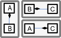
Figure 1: Three jointly inconsistent class diagrams

However, when three models work together, their consistency is a ternary relation often irreducible to binary consistency relations. Figure 1 presents a simple example: three class diagrams shown in the figure are pairwise consistent while the whole triple is obviously inconsistent, i.e., violates a class diagram metamodel constraint (which prohibits composition cycles).

A binary lens can be seen as a couple of Mealy machines (we write $A_{1}\rightleftarrows A_{2}$) sharing a state space (say, $R_{12}$). A ternary lens synchronizing a triple of models can also be seen as a triple of couples of Mealy machines ($A_{1}\rightleftarrows A_{2}$, $A_{1}\rightleftarrows A_{3}$, $A_{2}\rightleftarrows A_{3}$), but they share the same space $R_{123}$ and hence mutually dependant on each other (they would be independent if each couple $A_{i}\rightleftarrows A_{j}$would have its own space $R_{ij}$). Thus, multiple model synchronization is, in general, irreducible to chains of binary lenses and needs a new notion of a multiary lens.

2.0.2 2.2 Why amendments.

Getting back to the example, suppose that the updated state $A_{1}^{\prime}$ goes beyond the projection of all jointly consistent states to the space $A_{1}$, and hence consistency cannot be restored with the first model being in state $A^{\prime}_{1}$. When we work with two models, such cases could be a priori prohibited by modifying the corresponding metamodel $M_{1}$ defining the model space so that state $A^{\prime}_{1}$ would violate $M_{1}$. When the number of models to sync grows, it seems more convenient and realistic to keep $M_{1}$ more flexible and admitting $A^{\prime}_{1}$ but, instead, when the synchronizer is restoring consistency of all models, an amendment of state $A^{\prime}_{1}$ to a state $A^{\prime\prime}_{1}$ is also allowed. Thus, update propagation works reflectively so that not only other models are changed but the initiating update from $A_{1}$ to $A^{\prime}_{1}$ is itself amended and model $A^{\prime}_{1}$ is changed to $A^{\prime\prime}_{1}$. Moreover, in Sect. 3.3 we will consider examples of situations when if even state $A^{\prime}_{1}$ can be synchronized, a slight amendment still appears to be a better synchronization policy. For example, if consistency restoration with $A^{\prime}_{1}$ kept unchanged requires deletions in other models, while amending $A^{\prime}_{1}$ to $A^{\prime\prime}_{1}$ allows to restore consistency by using additions only, then the update policy with amendments may be preferable – as a rule, additions are preferable to deletions.

Of course, allowing for amendments may open the Pandora box of pathological synchronization scenarios, e.g., we can restore consistency by rolling back the original update and setting $A^{\prime\prime}_{1}=A_{1}$. We would like to exclude such solutions and bound amendments to work like completions of the updates rather than corrections and thus disallow any sort of “undoing”. To achieve this, we introduce a binary relation $\mathsf{K}^{{\blacktriangleright\!\!\blacktriangleright}}$ of update compatibility: if an update $u{:}\;A_{1}\rightarrow A^{\prime}_{1}$ is followed by update $v{:}\;A^{\prime}_{1}\rightarrow A_{1}^{\prime\prime}$ and $u\mathsf{K}^{{\blacktriangleright\!\!\blacktriangleright}}\,v$, then $v$ does not undo anything done by $u$. Then we require that the original update and its amendment be $\mathsf{K}^{{\blacktriangleright\!\!\blacktriangleright}}$-related. (Relation $\mathsf{K}^{{\blacktriangleright\!\!\blacktriangleright}}$ and its formal properties are discussed in Sect. 4.2.)

2.0.3 2.3 Why K-Putput.

An important and desired property of update propagation is its compatibility with update composition. If $u$ and $v$ are sequentially composable updates, and $\mathsf{put}$ is an update propagation operation, then its compositionality means $\mbox{$\mathsf{put}$}(u;v)=\mbox{$\mathsf{put}$}(u);\mbox{$\mathsf{put}$}(v)$ —hence, the name Putput for the law. There are other equational laws imposed on propagation operations in the lens framework  to guarantee desired synchronization properties and exclude unwanted scenarios. Amongst them, Putput is the most controversial: Putput without restrictions does not hold while finding an appropriate guarding condition – not too narrow to be practically usable and not too wide to ensure compositionality – has been elusive (cf. [15, 18, 10, 20, 6, 5]). The practical importance of Putput follows from the possibilities of optimizing update propagation it opens: if Putput holds, instead of executing two propagations, the engine can executes just one. Moreover, before execution, the engine can optimize the procedure by preprocessing the composed update $u;v$ and, if possible, converting it into an equivalent but easier manageable form (something like query optimization performed by database engines).

A preliminary idea of a constrained Putput is discussed in [20] under the name of a monotonic Putput: compositionality is only required for two consecutive deletions or two consecutive insertions (hence the term monotonic), which is obviously a too strong filter for typical practical applications. The idea of constraining Putput based on a compatibility relations over consecutive updates, e.g., relation $\mathsf{K}^{{\blacktriangleright\!\!\blacktriangleright}}$ above, is much more flexible, and gives the name K-Putput for the law. It was proposed by Orejas et al in [29] for the binary case without amendment and intermodel correspondences (more accurately, with trivial correspondences being just pairs of models), and we adapt it for the case of full-fledge lenses with general correspondences and amendments. We consider our integration of $\mathsf{K}^{{\blacktriangleright\!\!\blacktriangleright}}$-constrained Putput and amendments to be an important step towards making the lens formalism more usable and adaptable for practical tasks.

2.0.4 2.4 Why non-concurrent synchronization.

In the paper, we will consider consistency violation caused by a change of only one model, and thus consistency is restored by propagating only one update, while in practice we often deal with several models changing concurrently. If these updates are independent, the case can be covered with one-update propagation framework using interleaving, but if concurrent updates are in conflict, consistency restoration needs a conflict resolution operation (based on some policy) and goes beyond the framework we will develop in the paper. One reason for this is technical difficulties of building lenses with concurrency – we need to specify reasonable equational laws regulating conflict resolution and its interaction with update composition. It would be a new stage in the development of the lens algebra.

Another reason is that the case of one-update propagation is still practically interesting and covers a broad class of scenarios – consider a UML model developed by a software engineer. Indeed, different UML diagrams are just different views of a single UML model maintained by the tool, and when the engineer changes one of the diagrams, the change is propagated to the model and then the changed model is projected to other diagrams. Our construct of star-composition of lenses (see Sect. LABEL:sec:lego-star and Fig. LABEL:fig:starComposition) models exactly this scenario. Also, if a UML model is being developed by different teams concurrently, team members often agree about an interleaving discipline of making possibly conflicting changes, and the one-update framework is again useful. Finally, if concurrent changes are a priori known to be independent, this is well modelled by our construct of parallel composition of one-update propagating lenses (see Sect. 6.1).

2.0.5 2.5 Lens terminology.

The domain of change propagation is inherently complicated and difficult to model formally. The lens framework that approaches the task is still under development and even the basic concepts are not entirely settled and co-exist in several versions (e.g., there are strong and weak invertibility, several versions of Putput, and different names for the same property of propagating idle updates to idle updates). This results in a diverse collection of different types of lenses, each of which has a subtype of so called well-behaved (wb) lenses (actually, several such as the notion of being wb varies), which are further branched into different notions of very wb lenses depending on the Putput version accepted. The diversity of lens types and their properties, on the one hand, and our goal to provide accurate formal statements, on the other hand, would lead to overly wordy formulations. To make them more compact, we use two bracket conventions.

Square brackets. If we say A wb lens is called [weakly] invertible, when…, we mean that using adjective weakly is optional for this paper as the only type of invertibility we consider is the weak invertibility. However, we need to mention it because the binary lens notion that we generalize in our multiary lens notion, is the weak invertibility to be distinguished from the strong one. Thus, we mention ‘weakly’ in square brackets for the first time and then say just ‘invertible’ (except in a summarizing result like a theorem, in which we again mention [weakly]).

Round brackets. If a theorem reads A span of (very) wb asymmetric lenses … gives rise to a (very) wb symmetric lens … it mean that actually we have two versions of the theorem: one is for wb lenses, and the other is for very wb lenses.

3 Example

We will consider a simple example motivating our framework. The formal constructs constituting the multiary delta lesn framework  will be illustrated with the example (or its fragments) and referred to as Running example. Although the lens framework is formal, the running example instantiating it, will be presented semi-formally: we will try to be precise enough, but an accurate formalization would require the machinery of graphs with diagram predicates and partial graph morphisms as described in our paper [26], and we do not want to overload this paper with formalities even more.

3.1 A Multimodel to Play With

Suppose two data sources, whose schemas (we say metamodels) are shown in Fig. 2 as class diagrams $M_{1}$ and $M_{2}$  that record employment. The first source is interested in employment of people living in downtown, the second one is focused on software companies and their recently graduated employees. In general, population of classes $\mathsf{Person}$ and $\mathsf{Company}$ in the two sources can be different – they can even be disjoint, but if a recently graduated downtowner works for a software company, her appearance in both databases is very likely.

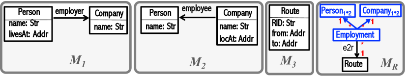
Figure 2: Multi-Metamodel in UML

Now suppose there is an agency investigating traffic problems, which maintains its own data on commuting routes between addresses as shown by schema $M_{3}$. These data should be synchronized with commuting data provided by the first two sources and computable by an obvious relational join over $M_{1}$ and $M_{2}$: roughly, the agency keeps traceability between the set of employment records and the corresponding commuting routes and requires their $\mathsf{from}$ and $\mathsf{to}$ attributes to be synchronized — below we will specify this condition in detail and explain the forth metamodel $M_{R}$ (see specification $(R_{123})$ on the next page). In addition, the agency supervises consistency of the two sources and requires that if they both know a person $p$ and a company $c$, then they must agree on the employment record $(p,c)$: it is either stored by both or by neither of the sources. For this synchronization, it is assumed that persons and companies are globally identified by their names. Thus, a triple of data sets (we will say models) $A_{1}$, $A_{2}$, $A_{3}$, instantiating the respective metamodels, can be either consistent (if the constraints described above are satisfied) or inconsistent (if they aren’t). In the latter case, we normally want to change some or all models to restore consistency. We will call a collection of models to be kept in sync a multimodel.

To specify constraints for multimodels in an accurate way, we need an accurate notation. If $A$ is a model instantiating metamodel $M$ and $X$ is a class in $M$, we write $X^{A}$ for the set of objects instantiating $X$ in $A$. Similarly, if $r\!:X_{1}\leftrightarrow X_{2}$ is an association in $M$, we write $r^{A}$ for the corresponding binary relation over $X_{1}^{A}\times X_{2}^{A}$. For example, Fig. 3 presents a simple model $A_{1}$ instantiating $M_{1}$ with $\mathsf{Person}^{A_{1}}=\{p_{1},p_{1}^{\prime}\}$, $\mathsf{Company}^{A_{1}}=\{c_{1}\}$, $\mathsf{employer}^{A_{1}}=\{(p_{1},c_{1})\}$, and similarly for attributes, e.g.,

$$\mathsf{livesAt}^{A_{1}}=\{(p_{1},a1),(p^{\prime}_{1},a1)\}\subset\mathsf{Person}^{A_{1}}{\times}\mathsf{Addr}$$

($\mathsf{livesAt}^{A_{1}}$ and also $\mathsf{name}^{A_{1}}$ are assumed to be functions and $\mathsf{Addr}$ is the (model-independent) set of all possible addresses). Two other boxes present models $A_{2}$ and $A_{3}$ instantiating metamodels $M_{2}$ and $M_{3}$ resp.; we will discuss the rightmost box $R$ later. The triple $({A_{1}},{A_{2}},{A_{3}})$ is a (state of the) multimodel over the multimetamodel $(M_{1},M_{2},M_{3})$, and we say it is consistent if the constraints specified below are satisfied.

Constraint (C1) specifies mutual consistency of models $A_{1}$ and $A_{2}$ in the sense described above:

(C1)	if $p\in\mathsf{Person}^{A_{1}}\cap\mathsf{Person}^{A_{2}}$ and $c\in\mathsf{Company}^{A_{1}}\cap\mathsf{Company}^{A_{2}}$
	then $(p,c)\in\mathsf{employer}^{A_{1}}$ iff $(c,p)\in\mathsf{employee}^{A_{2}}$

Our other constraints specify consistency between the agency’s data on commuting routes and the two data sources. We first assume a new piece of data that relates models: a relation $\mathsf{(e2r)}^{R}$ whose domain is the integral set of employment records $\mathsf{Employment}^{{A_{1}}{*}{A_{2}}}$ as specified below in ($R_{123}$):

($R_{123}$)	$\mathsf{(e2r)}^{R}\subset\mathsf{Employment}^{{A_{1}}{*}{A_{2}}}\times\mathsf{Route}^{A_{3}}$
	where $\mathsf{Employment}^{{A_{1}}{*}{A_{2}}}\stackrel{{\scriptstyle\mathrm{def}}}{{=}}{\mathsf{employer}^{A_{1}}\cup{(\mathsf{employee}^{A_{2}})}^{-1}}$

This relation is described in the metamodel $M_{R}$ in Fig. 2, where blue boxes denote (derived) classes whose instantiation is to be automatically computed (as specified above) rather than is given by the user.

To simplify presentation, we assume that all employees commute rather than work from home, which means that relation $\mathsf{(e2r)}^{R}$ is left-total. Another simplifying assumption is that each employment record maps to exactly one commuting route, hence, relation $\mathsf{(e2r)}^{R}$ is a single-valued mapping. Finally, several people living at the same address may work for the same company, which leads to different employment records mapped to the same route and thus injectivity is not required. Hence, we have the following intermodel constraint:

(C2)	relation $\mathsf{(e2r)}^{R}$ is a total function ${\mathsf{Employment}^{{A_{1}}{*}{A_{2}}}}\longrightarrow{\mathsf{Route}^{A_{3}}}$

which is specified in the metamodel $M_{R}$ in Fig. 2 by the corresponding multiplicities. However, the metamodel $M_{R}$ as shown in Fig. 2, is still an incomplete specification of correspondences between models.

For each employment record $e\in\mathsf{Employment}^{{A_{1}}{*}{A_{2}}}$, there are defined the corresponding person

$$p=e.\mathsf{employee}^{{A_{1}}{*}{A_{2}}}\in\mathsf{Person}^{{A_{1}}{*}{A_{2}}}\stackrel{{\scriptstyle\mathrm{def}}}{{=}}\mathsf{Person}^{A_{1}}\cup\mathsf{Person}^{A_{2}}$$

with attribute

$$p.\mathsf{livesAt}^{{A_{1}}{*}{A_{2}}}=\left\{\begin{array}[]{ll}p.\mathsf{livesAt}^{A_{1}}&\mbox{if $p\in\mathsf{Person}^{A_{1}}$,}\\[4.30554pt] \bot&\mbox{otherwise.}\end{array}\right.$$

We thus assume that the domain $\mathsf{Addr}$ is extended with a bottom value/null $\bot$. Similarly, we define set $\mathsf{Company}^{{A_{1}}{*}{A_{2}}}$ with attribute $\mathsf{locAt}^{{A_{1}}{*}{A_{2}}}$ and the corresponding “end” $e.\mathsf{employer}^{{A_{1}}{*}{A_{2}}}\in\mathsf{Company}^{{A_{1}}{*}{A_{2}}}$ for any employment record $e$. The latter is of special interest for the agency if both addresses,

$$e.\mathsf{employee}^{{A_{1}}{*}{A_{2}}}.\mathsf{livesAt}^{{A_{1}}{*}{A_{2}}}\mbox{ and }e.\mathsf{employer}^{{A_{1}}{*}{A_{2}}}.\mathsf{locAt}^{{A_{1}}{*}{A_{2}}},$$

are defined and thus define a certain commuting route to be consistent with its image $e.\mathsf{(e2r)}^{R}$ in $\mathsf{Route}^{A_{3}}$.

More generally, the consistency of the two sets of commuting routes: that one derived from $A_{1}$ and $A_{2}$, and that one stored in $A_{3}$, can be specified as follows:

(C3)	$e.\mathsf{employee}^{{A_{1}}{*}{A_{2}}}.\mathsf{livesAt}^{{A_{1}}{*}{A_{2}}}$	$\leq e.\mathsf{(e2r)}^{R}.\mathsf{from}^{A_{3}}$
	$e.\mathsf{employer}^{{A_{1}}{*}{A_{2}}}.\mathsf{locAt}^{{A_{1}}{*}{A_{2}}}$	$\leq e.\mathsf{(e2r)}^{R}.\mathsf{to}^{A_{3}}$

where inequality $a_{1}\leq a_{2}$ holds iff both values are certain and $a_{1}=a_{2}$, or both values are nulls, or $a_{1}$ is a null while $a_{2}$ is certain.

Now it is easy to see that multimodel $(A_{1},A_{2},A_{3},R)$ in Fig. 3 is “two-times” inconsistent: (C1) is violated as both $A_{1}$ and $A_{2}$ know Mary and IBM, and (IBM,Mary)$\in$ $\mathsf{employee}^{A_{2}}$ but (Mary, IBM)$\notin\mathsf{employer}^{A_{1}}$, and (C2) is violated as $A_{2}$ and $R$ show an employment record $e_{2}$ not mapped to a route in $\mathsf{Route}^{A_{3}}$. Note also that if we map this record to the route #1 to fix (C2), then constraint (C3) will be violated. We will discuss consistency restoration in the next subsection, but first we need to finish our discussion of intermodel correspondences.

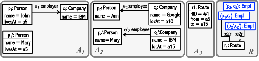
Figure 3: Multimodel ${\cal A}^{\dagger}=(A_{1},A_{2},A_{3},R)$ with $\mathsf{(p2p)}^{R}=\{(p_{1}^{\prime},p_{2}^{\prime})\}$, $\mathsf{(c2c)}^{R}=\{(c_{1},c_{2}^{\prime})\}$, and $\mathsf{(e2r)}^{R}=\{(e_{1},r_{1}),({e^{\prime}_{2}}^{-1},r_{1})\}$

Note that correspondences between models have more data than specified in ($R_{123}$). Indeed, classes $\mathsf{Person}^{A_{1}}$ and $\mathsf{Person}^{A_{2}}$ are interrelated by a correspondence linking persons with the same name, and similarly for $\mathsf{Company}$ so that we have two partial injections:

($R_{12}$)

$\mathsf{(p2p)}^{R}\subset\mathsf{Person}^{A_{1}}{\times}\mathsf{Person}^{A_{2}}$, $\mathsf{(c2c)}^{R}\subset\mathsf{Company}^{A_{1}}{\times}\mathsf{Company}^{A_{2}}$,

which are not shown in metamodel $M_{R}$ (by purely technical reasons of keeping the figure compact and fitting in the page width). These correspondence links (we will write corr-links) may be implicit as they can always be restored using names as keys. In contrast, relation $\mathsf{(e2r)}$ is not determined by the component model states $A_{1},A_{2},A_{3}$ and is an independent piece of data. Importantly, for given models $A_{1,2,3}$, there may be several different correspondence mappings $\mathsf{(e2r)}^{R}$ satisfying the constraints. For example, if there are several people living at the same address and working for the same company, all employment record can be mapped to the same route or to several different routes depending on how much carpooling is used. In fact, multiplicity of possible corr-specifications is a general story; it can happen for relations $\mathsf{(p2p)}$ and $\mathsf{(c2c)}$ as well if person and company names are not entirely reliable keys. Then we need a separate procedure of model matching or alignment that has to establish, e.g., whether objects $p^{\prime}_{1}\in\mathsf{Person}^{A_{1}}$ and $p^{\prime}_{2}\in\mathsf{Person}^{A_{2}}$ both named Mary represent the same real world object. Constraints we declared above implicitly involve corr-links, e.g., formula for (C1) is a syntactic sugar for the following formal statement: if $(p_{1},p_{2})\in\mathsf{(p2p)}^{R}$ and $(c_{1},c_{2})\in\mathsf{(c2c)}^{R}$ with $p_{i}{\in}\mathsf{Person}^{A_{i}}$, $c_{i}{\in}\mathsf{Company}^{A_{i}}$ ($i=1,2$), then the following holds: $(p_{1},c_{1})\in\mathsf{employer}^{A_{1}}$ iff $(c_{2},p_{2})\in\mathsf{employee}^{A_{2}}$. A precise formal account of this discussion can be found in [26].

Thus, a multimodel is actually a tuple ${\cal A}=({A_{1}},{A_{2}},{A_{3}},R)$ where $R$ is a correspondence specification (which, in our example, is a collection of correspondence relations ($R_{123}$), ($R_{12}$) over sets involved). Consistency of a multimodel is a property of the entire 4-tuple ${\cal A}$ rather than its 3-tuple carrier $({A_{1}},{A_{2}},{A_{3}})$.

3.2 Synchronization via Update Propagation

There are several ways to restore consistency of the multimodel in Fig. 3 w.r.t. constraint (C1). We may delete Mary from $A_{1}$, or delete her employment with IBM from $A_{2}$, or even delete IBM from $A_{2}$. We can also change Mary’s employment from IBM to Google, which will restore (C1) as $A_{1}$ does not know Google. Similarly, we can delete John’s record from $A_{1}$ and then Mary’s employment with IBM in $A_{2}$ would not violate (C1). As the number of constraints and the elements they involve increase, the number of consistency restoration variants grows fast.

The range of possibilities can be essentially decreased if we take into account the history of creating inconsistency and consider not only an inconsistent state ${\cal A}^{\dagger}$ but update $u{:}\;{\cal A}\rightarrow{\cal A}^{\dagger}$ that created it (assuming that ${\cal A}$ is consistent). For example, suppose that initially model $A_{1}$ contained record (Mary, IBM) (and $A_{3}$ contained (a1, a15)-commute), and the inconsistency appears after Mary’s employment with IBM was deleted in $A_{1}$. Then it’s reasonable to restore consistency by deleting this employment record in $A_{2}$ too; we say that deletion was propagated from $A_{1}$ to $A_{2}$. If the inconsistency appears after adding (IBM, Mary)-employment to $A_{2}$, then it’s reasonable to restore consistency by adding such a record to $A_{1}$. Although propagating deletions/additions to deletions/additions is typical, there are non-monotonic cases too. Let us assume that Mary and John are spouses and live at the same address, and that IBM follows an exotic policy prohibiting spouses to work together. Then we can interpret addition of (IBM, Mary)-record to $A_{2}$ as swapping of the family member working for IBM, and then (John, IBM) is to be deleted from $A_{1}$.

Now let’s consider how updates to and from model $A_{3}$ may be propagated. As mentioned above, traceability/correspondence links play a crucial role here. If additions to $A_{1}$ or $A_{2}$ create a new commute, the latter has to be added to $A_{3}$ (together with its corr-links) due to constraints (C2) and (C3). In contrast, if a new route is added to $A_{3}$, we may change nothing in $A_{1,2}$ as (C2) does not require surjectivity of $\mathsf{(e2r)}$ (but further in the paper we will consider a more intricate policy). If a route is deleted from $A_{3}$, and it is traced via $\mathsf{(e2r)}^{R}$ to one or several corresponding employments in $\mathsf{Employment}^{{A_{1}}{*}{A_{2}}}$, then they are either deleted too, or perhaps remapped to other routes with the same $\mathsf{from}$-$\mathsf{to}$pair of attributes if such exist. Similarly, deletions in $\mathsf{Employment}^{{A_{1}}{*}{A_{2}}}$ may (but not necessarily) lead to the corresponding deletions in $\mathsf{Route}^{A_{3}}$ depending on the mapping $\mathsf{(e2r)}^{R}$. Finally, updating addresses in $A_{1}$ or $A_{2}$ is propagated to the corresponding updates of $\mathsf{from}$ and $\mathsf{to}$ attributes in $A_{3}$ to satisfy constraint (C3); similarly for attribute updates in $A_{3}$.

Clearly, many of the propagation policies above although formally correct, may contradict the real world changes and hence should be corrected, but this is a common problem of a majority of automatic synchronization approaches, which have to make guesses in order to resolve non-determinism inherent in consistency restoration.

3.3 Reflective Update Propagation

An important feature of update propagation scenarios above is that consistency could be restored without changing the model whose update caused inconsistency. However, this is not always desirable. Suppose again that violation of constraint (C1) in multimodel in Fig. 3 was caused by adding a new person Mary to $A_{1}$, e.g., as a result of Mary’s moving to downtown. Now both models know both Mary and IBM, and thus either employment record (Mary, IBM) is to be added to $A_{1}$, or record (IBM, Mary) is to be removed from $A_{2}$. Either of the variants is possible, but in our context, adding (Mary, IBM) to $A_{1}$ seems more likely and less specific than deletion (IBM, Mary) from $A_{2}$. Indeed, if Mary has just moved to downtown, the data source $A_{1}$ simply may not have completed her record yet. Deletion (IBM, Mary) from $A_{2}$ seems to be a different event unless there are strong causal dependencies between moving to downtown and working for IBM. Thus, an update policy that would keep $A_{2}$ unchanged but amend addition of Mary to $A_{1}$ with further automatic adding her employment for IBM (as per model $A_{2}$) seems reasonable. This means that updates can be reflectively propagated (we also say self-propagated).

Of course, self-propagation does not necessarily mean non-propagation to other directions. Consider the following case: model $A_{1}$ initially only contains (John, IBM) record and is consistent with $A_{2}$ shown in Fig. 3. Then record (Mary, Google) was added to $A_{1}$, which thus became inconsistent with $A_{2}$. To restore consistency, (Mary, Google) is to be added to $A_{2}$ (the update is propagated from $A_{1}$ to $A_{2}$) and (Mary, IBM) to be added to $A_{1}$ as discussed above (i.e., addition of (Mary, Google) is both amended and propagated). Note, however, that in contrast to the previous case, now deletion of the record (IBM, Mary) from $A_{2}$  looks like an equally reasonable scenario of Mary changing her employer. Thus, even for the simple case above, and the more complex cases of model interaction, the choice of the update policy (only amend, only propagate, or both) depends on the context, heuristics, and tuning the policy to practice.

A typical situation that needs an amendment facility is when the changes in interacting models have different granularity. With our simple running example, we can illustrate the point in the following (rather artificial) way. Suppose, again, that the record of Mary working for Google, and her address unknown (i.e., Mary.$\mathsf{livesAt}=\bot$) is added to model $A_{1}$, and propagated to $A_{2}$ as discussed above. Suppose that Google has a strict policy of only hiring those recent graduates who live on Bloor Street in Toronto downtown. Then in Mary’s address record, all fields could (and should!) be made certain besides the street number. Hence, adding Mary’s employment to model $A_{1}$ should be amended with extending her address with data imposed by model $A_{2}$. For a more realistic example, consider model $A_{2}$ specifying a complex engineering project $P$ in the process of elaboration, while model $A_{1}$ gives its very abstract view – the budget $B$ of the project. If the budget changes from $B$ to $B^{\prime}$, the project should also be changed, but it is very likely that the budget of the changed project $P^{\prime}$ would be $B^{\prime\prime}$ rather than exactly $B^{\prime}$. A more general and formal description of this synchronization schema can be found in [5].

3.4 General schema

Figure 4: Update propagation pattern (To distinguish given data from those produced by the operation, the former are shown with framed nodes and solid lines, while the latter are non-framed and dashed.)

A general schema of update propagation including reflection is shown in Fig. 4. We begin with a consistent multimodel $({A_{1}}...A_{n},R)$ one of which members is updated $u_{i}{:}\;A_{i}\rightarrow A^{\prime}_{i}$. The propagation operation, based on a priori defined propagation policies as sketched above, produces:

a) updates on all other models $u^{\prime}_{j}{:}\;A_{j}\rightarrow A^{\prime\prime}_{j}$, $1\leq j\neq i\leq n$;

b) an amendment $u_{i}^{@}{:}\;A^{\prime}_{i}\rightarrow A^{\prime\prime}_{i}$ to the original update;

c) a new correspondence specification $R^{\prime\prime}$ such that the updated multimodel

$\qquad(A^{\prime\prime}_{1}...A^{\prime\prime}_{n},R^{\prime\prime})$

is consistent.

Below we introduce an algebraic model encompassing several operations and algebraic laws formally modelling situations considered so far.

4 Multimodel spaces

In this section we begin to build a formal framework for delta lenses: model spaces are described as categories whose objects are models and arrows are updates, which carry several additional relations and operations. We also abstractly define correspondences between models and our central notion of a (consistent) multimodel. We will follow an established terminological tradition (in the lens community) to give, first, a name to an algebra without any equational requirement, and then call an algebra satisfying certain equations well-behaved.

4.1 Background: Graphs, (co)Spans, and Categories

We reproduce well-known definitions to fix our notation. A (directed multi-)graph $G$ consists of a set $\mathsf{Ob}(G)$ of nodes and a set $\mathsf{Ar}(G)$ of arrows equipped with two functions $\mathsf{s},\mathsf{t}{:}\;\mathsf{Ar}(G)\rightarrow\mathsf{Ob}(G)$ that give arrow $a$ its source $\mathsf{s}(a)$ and target $\mathsf{t}(a)$ nodes. We write $a{:}\;N\rightarrow N^{\prime}$ if $\mathsf{s}(a)=N$ and $\mathsf{t}(a)=N^{\prime}$, and $a{:}\;N\rightarrow\_$ or $a{:}\;\_\rightarrow N^{\prime}$ if only one of these conditions is given.

Expressions $G(N,N^{\prime})$, $G(N,\_)$, $G(\_,N^{\prime})$ denote sets of, resp., all arrows from $N$ to $N^{\prime}$, all arrows from $N$, and all arrows into $N^{\prime}$.

A pair of arrows $a_{i}{:}\;N\rightarrow N^{\prime}_{i}$, $i=1,2$, with a common source is called a [binary] span with node $N$ its head or apex, nodes $N^{\prime}_{i}$ feet, and arrows $a_{i}$ legs. Dually, a pair of arrows $a_{i}\!:N\leftarrow N^{\prime}_{i}$, $i=1,2$, with a common target is called a (binary) cospan with apex, feet, and legs, defined similarly.

A [small] category is a graph, whose nodes are called objects, arrows are associatively composable, and every object has a special identity loop, which is the unit of the composition. In more detail, given two consecutive arrows $a_{1}{:}\;\_\rightarrow N$ and $a_{2}{:}\;N\rightarrow\_$, we denote the composed arrow by $a_{1};a_{2}$. The identity loop of node $N$ is denoted by $\mathsf{id}_{N}$, and equations $a_{1};\mathsf{id}_{N}=a_{1}$ and $\mathsf{id}_{N};a_{2}=a_{2}$ are to hold. We will denote categories by bold letters, say, $\mathbf{A}$, and often write $A\in{\mathbf{A}}$ rather than $A\in\mathsf{Ob}(\mathbf{A})$ for its objects.

A functor is a mapping of nodes and arrows from one category to another, which respects sources and targets as well as identities and composition. Having a tuple/family of categories $\mathbf{A}=(\mathbf{A}_{1}...\mathbf{A}_{n})$, their product is a category $\prod\!\mathbf{A}=\mathbf{A}_{1}{\times}...{\times}\mathbf{A}_{n}$ whose objects are tuples ${A}=(A_{1}...A_{n})\in\mathsf{Ob}(\mathbf{A}_{1}){\times}...{\times}\mathsf{Ob}(\mathbf{A}_{n})$, and arrows from $(A_{1}...A_{n})$ to $(A^{\prime}_{1}...A^{\prime}_{n})$ are tuples of arrows ${u}=(u_{1}...u_{n})$ with $u_{i}{:}\;A_{i}\rightarrow A^{\prime}_{i}$ for all $i=1...n$.

4.2 Model Spaces and updates

Basically, a model space is a category, whose nodes are called model states or just models, and arrows are (directed) deltas or updates. For an arrow $u{:}\;A\rightarrow A^{\prime}$, we treat $A$ as the state of the model before update $u$, $A^{\prime}$ as the state after the update, and $u$ as an update specification. Structurally, it is a specification of correspondences between $A$ and $A^{\prime}$. Operationally, it is an edit sequence (edit log) that changed $A$ to $A^{\prime}$. The formalism does not prescribe what updates are, but assumes that they form a category, i.e., there may be different updates from state $A$ to state $A^{\prime}$; updates are composable; and idle updates $\mathsf{id}_{A}{:}\;A\rightarrow A$ (doing nothing) are the units of the composition. A prominent example of model spaces is the category of graphs where updates are encoded as (certain equivalence classes of) binary spans between them. They are heavily used in the theory of Graph Transformations [13]. In this way an update $u:A\to A^{\prime}$ can be a deletion or an addition or a combination of both.

We require every model space $\mathbf{A}$ to be endowed with two additional constructs of update compatibility.

4.2.1 Sequential compatibility of updates

We assume a family $(\mathsf{K}^{{\blacktriangleright\!\!\blacktriangleright}}_{A})_{A{\in}\mathsf{Ob}(\mathbf{A})}$ of binary relations $\mathsf{K}^{{\blacktriangleright\!\!\blacktriangleright}}_{A}\subset{\mathbf{A}}(\_,A){\times}{\mathbf{A}}(A,\_)$ indexed by objects of $\mathbf{A}$, and specifying non-conflicting or compatible consecutive updates. Intuitively, an update $u$ into $A$ is compatible with update $u^{\prime}$ from $A$, if $u^{\prime}$ does not revert/undo anything done by $u$, e.g., it does not delete/create objects created/deleted by $u$, or re-modify attributes modified by $u$. For example, one could add Mary’s employment at IBM ($u{:}\;A_{1}\rightarrow A_{1}^{\prime}$) and subsequently add Ann ($u^{\prime}{:}\;A_{1}^{\prime}\rightarrow A_{1}^{\prime\prime}$) to $A^{\prime}_{1}$ yielding a pair $(u,u^{\prime})\in\mathsf{K}^{{\blacktriangleright\!\!\blacktriangleright}}_{A_{1}^{\prime}}$ (see [29] for a detailed discussion). Later we will specify several formal requirements to the compatibility (see Def. 2 below).

(1) $$\begin{diagram}$$

Figure 5: Update merging

4.2.2 Concurrent compatibility of updates and their merging

Intuitively, a pair of updates $u=(u_{1},u_{2})$ from a common source $A$ (i.e., a span) as shown in Fig. 5 diagram (1) is called concurrently compatible, if it can be performed in either order leading to the same result – an update $u_{1}+u_{2}{:}\;A\rightarrow A^{\prime\prime}$. Formally, in the case of concurrent compatibility of $u_{1}$ and $u_{2}$, we require the existence of update $u_{1}+u_{2}{:}\;A\rightarrow A^{\prime\prime}$ and updates $\tilde{u_{i}}{:}\;A_{i}^{\prime}\rightarrow A^{\prime\prime}$ such that $u_{1};\tilde{u_{1}}=u_{2};\tilde{u_{2}}=u_{1}+u_{2}$. Then we call updates $u_{i}$ mergeable, update $u_{1}+u_{2}$ their merge, and updates $\tilde{u_{1}},\tilde{u_{2}}$ complements, and write $(\tilde{u_{1}},\tilde{u_{2}})=\mathsf{merge}_{A}(u_{1},u_{2})$ or else $\tilde{u_{i}}=\mathsf{merge}_{A,i}(u_{1},u_{2})$. We will also denote the model $A^{\prime\prime}$ by $A^{\prime}_{1}+_{A}A^{\prime}_{2}$. For example, for model $A_{1}$ in Fig.3, we can concurrently delete John’s and add Mary’s employments with IBM, or concurrently add two Mary’s employments, say, with IBM and Google. But deleting Mary from the model and adding her employment with IBM are not concurrently compatible. Similarly, in $A_{3}$, updating addresses of different routes, or updating the $\mathsf{from}$ and $\mathsf{to}$ attributes of the same route are concurrently compatible, but deleting a route and changing its attributes are incompatible (we will also say, in conflict). We denote the set of all mergeable spans with apex $A$ by $\mathsf{K}^{{\blacktriangle{}}}_{A}$.

The definition of concurrent compatibility is a generalization of the notion of parallel independence of graph transformation rules [12]. Below we will elaborate further on the interplay of sequentially and concurrently compatible pairs.

Now we can define model spaces.

Definition 1 (Model Spaces)

A model space is a tuple

$$\mathbf{A}=(|\mathbf{A}|,\mathsf{K}^{{\blacktriangleright\!\!\blacktriangleright}},\mathsf{K}^{{\blacktriangle{}}},\mathsf{merge})$$

of the following four components. The first one is a category |$\mathbf{A}$| (the carrier) of models and updates. We adopt a notational convention to omit the bars $|$ and denote a space and its carrier category by the same symbol $\mathbf{A}$. The second component is a family

$$\mathsf{K}^{{\blacktriangleright\!\!\blacktriangleright}}=\left(\mathstrut{\mathsf{K}^{{\blacktriangleright\!\!\blacktriangleright}}_{A}\subset\mathbf{A}(\_,A){\times}\mathbf{A}(A,\_)}\,|\;{A{\in}\mathsf{Ob}(\mathbf{A})}\right)$$

of sequential compatibility relations for sequential update pairs as described above. The third and forth component are tightly coupled:

$$\mathsf{K}^{{\blacktriangle{}}}=\left(\mathstrut{\mathsf{K}^{{\blacktriangle{}}}_{A}\subset\mathbf{A}(A,\_){\times}\mathbf{A}(A,\_)}\,|\;{A{\in}\mathsf{Ob}(\mathbf{A})}\right)$$

is a family of concurrently compatible or mergeable spans of updates, and

$$\mathsf{merge}=\left(\mathstrut{\mathsf{merge}_{A}}\,|\;{A{\in}\mathsf{Ob}(\mathbf{A})}\right)$$

is a family of merge operations as shown in (1). The domain of operation $\mathsf{merge}_{A}$ is exactly the set $\mathsf{K}^{{\blacktriangle{}}}_{A}$. We will denote the components of merge by $\mathsf{merge}_{A,i}$ with $i=1,2$ and omit index $A$ if they are clear from the context or not important. Writing $\mathsf{merge}_{A}(u_{1},u_{2})$ implicitly assumes $(u_{1},u_{2})\in\mathsf{K}^{{\blacktriangle{}}}_{A}$. ∎

Definition 2 (Well-behaved Model Spaces)

$\mathsf{{(\mathsf{K}^{{\blacktriangleright\!\!\blacktriangleright}}\ and\leavevmode\nobreak\ Id)}}$	For all $u{\in}{\mathbf{A}}(\_,A)$, $u^{\prime}{\in}{\mathbf{A}}(A,\_)$: $(u,\mathsf{id}_{A}),(\mathsf{id}_{A},u^{\prime}){\in}\mathsf{K}^{{\blacktriangleright\!\!\blacktriangleright}}_{A}$,
	For any three consecutive updates $u,v,w$, we require:
$\mathsf{{(\mathsf{K}^{{\blacktriangleright\!\!\blacktriangleright}}\mathsf{K}^{{\blacktriangleright\!\!\blacktriangleright}})}}_{1}$	$(u\mathsf{K}^{{\blacktriangleright\!\!\blacktriangleright}}\,vw$ $\wedge$ $v\mathsf{K}^{{\blacktriangleright\!\!\blacktriangleright}}w)$ imply $(u\mathsf{K}^{{\blacktriangleright\!\!\blacktriangleright}}v$ $\wedge$ $uv\,\mathsf{K}^{{\blacktriangleright\!\!\blacktriangleright}}w)$,
$\mathsf{{(\mathsf{K}^{{\blacktriangleright\!\!\blacktriangleright}}\mathsf{K}^{{\blacktriangleright\!\!\blacktriangleright}})}}_{2}$	$(uv\,\mathsf{K}^{{\blacktriangleright\!\!\blacktriangleright}}w$ $\wedge$ $u\mathsf{K}^{{\blacktriangleright\!\!\blacktriangleright}}v)$ imply $(v\mathsf{K}^{{\blacktriangleright\!\!\blacktriangleright}}w$ $\wedge$ $u\mathsf{K}^{{\blacktriangleright\!\!\blacktriangleright}}\,vw)$,
	where composition is denoted by concatenation ($uv$ for $u;v$ etc).
$\mathsf{{(\mathsf{K}^{{\blacktriangle{}}}\leavevmode\nobreak\ and\leavevmode\nobreak\ \mathsf{K}^{{\blacktriangleright\!\!\blacktriangleright}})}}$	For all $(u_{1},u_{2})\in\mathsf{K}^{{\blacktriangle{}}}_{A}$: $(u_{i},\widetilde{u_{i}})\in\mathsf{K}^{{\blacktriangleright\!\!\blacktriangleright}}_{A^{\prime}_{i}}$, $i=1,2$, where $\widetilde{u_{i}}=\mathsf{merge}_{A,i}(u_{1},u_{2})$
$\mathsf{{(MergeSym)}}$	For all $u_{1}{:}\;A\rightarrow A^{\prime}_{1}$, $u_{2}{:}\;A\rightarrow A^{\prime}_{2}$, if $(\widetilde{u_{1}},\widetilde{u_{2}})=\mathsf{merge}_{A}(u_{1},u_{2})$,
	then $(\widetilde{u_{2}},\widetilde{u_{1}})=\mathsf{merge}_{A}(u_{2},u_{1})$
$\mathsf{{(MergeId)}}$	For all $u{:}\;A\rightarrow A^{\prime}$: $\mathsf{merge}_{A}(u,\mathsf{id}_{A})=(\mathsf{id}_{A^{\prime}},u)$

∎

The first condition is the already discussed natural property for sequential compatibility. The pair of conditions below it requires complementing updates not to revert anything done by the other update. The last three conditions are obvious requirements to the operation $\mathsf{merge}$.

We assume all our model spaces to be wb and, as a rule, will omit explicit mentioning. Each of the metamodels $M_{1}$..$M_{3}$ in the running example gives rise to a (wb) model space of its instances as discussed above.

4.3 Correspondences and Multimodels

We will work with families of model spaces indexed by a finite set $I$, whose elements can be seen as space names. To simplify notation, we will assume that $I=\{1,\ldots,n\}$ although ordering will not play any role in our framework. Given a tuple of model spaces $\mathbf{A}_{1},\ldots,\mathbf{A}_{n}$, we will refer to objects and arrows of the product category $\prod\mathbf{A}=\mathbf{A}_{1}{\times}\cdots{\times}\mathbf{A}_{n}$ as tuple models and tuple updates, and denote them by letters without indexes, e.g., ${u}{:}\;{A}\rightarrow{A}^{\prime}$ is a family $u_{i}{:}\;A_{i}\rightarrow A^{\prime}_{i}$, $i=1..n$. We will call components of tuple models and updates their feet. We also call elements of a particular space $\mathbf{A}_{i}$ foot models and foot updates.

Definition 3 (Multispaces, Alignment, Consistency)

Let $n\geq 2$ be a natural number. An n-ary multi-space is a triple ${\boldsymbol{\mathcal{A}}}=(\mathbf{A},\mathsf{Corr},\partial)$ with the following components. The first one is a tuple of (wb) model spaces $\mathbf{A}=(\mathbf{A}_{1},\ldots,\mathbf{A}_{n})$ called the boundary of ${\boldsymbol{\mathcal{A}}}$. The other two components is a class $\mathsf{Corr}$ of elements called (consistent) correspondences or corrs, and a family of boundary mappings $\partial=\left(\mathstrut{\partial_{i}{:}\;\mathsf{Corr}\rightarrow\mathsf{Ob}(\mathbf{A}_{i})}\,|\;{i=1..n}\right)$.

A corr $R\in\mathsf{Corr}$ is understood as a correspondence specification interrelating models $A_{i}=\partial_{i}R$; the latter are also called R’s feet, and we say that models $A_{i}$ are aligned via $R$. We write $\partial R$ for the tuple $(\partial_{1}R...\partial_{n}R)$. When we consider several multispaces and need an explicit reference, we will write $\boldsymbol{\partial}$${\boldsymbol{\mathcal{A}}}$ for the boundary $\mathbf{A}$ of the entire multispace, and $\mathsf{Corr}({\boldsymbol{\mathcal{A}}})$ for its class of corrs.

Given a model tuple $A=(A_{1}...A_{n})\in\mathsf{Ob}((\prod\mathbf{A}))$, we write $\mathsf{Corr}(A)$ for the set $\left\{{R\in\mathsf{Corr}}|\;{\partial R=A}\right\}$, and $\mathsf{Corr}(A_{i})$ for the class $\left\{{R\in\mathsf{Corr}}|\;{\partial_{i}R=A_{i}}\right\}$; thus, $\mathsf{Corr}(A)=\bigcap_{i=1..n}\mathsf{Corr}(A_{i})$.

Although in this paper all corrs are considered consistent by default, we will often mention their consistency explicitly to recall the context and to ease comparison with similar but a bit more general frameworks, in which inconsistent corrs are also considered [11, 6]. ∎

Definition 4 (Multimodels)

A (consistent) multimodel over a multispace ${\boldsymbol{\mathcal{A}}}$ is a couple ${\cal A}=(A,R)$ of a model tuple ${A}=(A_{1}..A_{n})$ with a (consistent) corr $R\in\mathsf{Corr}({A})$ relating the component models. A multimodel update $\mathbf{u}{:}\;{\cal A}\rightarrow{\cal A}^{\prime}$ is a pair $(u,(R,R^{\prime}))$, whose first component is a tuple update $u=\left(\mathstrut{u_{i}{:}\;\partial_{i}R\rightarrow\partial_{i}R^{\prime}}\,|\;{i=1..n}\right)$, and the second component is a pair of the old and the new corrs. Identity updates are pairs $(\mathsf{id},(R,R))$, whose tuple component consists of identities $\mathsf{id}_{\partial_{i}R}$, $i=1..n$, only. It is easy to check that so defined multimodels and their updates determine a category that we denote by ${\boldsymbol{\mathcal{R}}}$. ∎

Remark 1

The notions of a corr and a multimodel are actually synonyms: any corr $R$ is simultaneously a multimodel $(\partial R,R)$, and any multimodel $(A,R)$ is basically just a corr $R$ as the feet part of the notion is uniquely restored by setting $A=\partial R$, thus, $\mathsf{Corr}\cong\mathsf{Ob}({\boldsymbol{\mathcal{R}}})$. We can extend the equivalence to arrows too by defining corr updates exactly as we defined multimodel updates. This would make class $\mathsf{Corr}$ into a category $\mathbf{Corr}$ isomorphic to ${\boldsymbol{\mathcal{R}}}$. Using two symbols and two names for basically the same notion is, perhaps, confusing but we decided to keep them to keep track of the historical use of the terminology. The choice of the word depends on the context: if we focus on the $R$ component of pair $(A,R)$, we say “corr”, if we focus on the $A$ component, we say “multimodel”.

Thus, for this paper, multimodel updates are basically tuple updates $u$ while their corr-component $(R,R^{\prime})$ is trivial (co-discrete in the categorical jargon) and so we actually will not need the category $\mathbf{Corr}$ (or ${\boldsymbol{\mathcal{R}}}$) explicitly declared. However, the notion will be useful when we will discuss categorification of the framework in Future Work Sect. LABEL:sec:future.1, and in Related Work Sect. LABEL:sec:related.

Example 1

The Running example of Sect.3 gives rise to a 3-ary multimodel space. For $i=1..3$, space $\mathbf{A}_{i}$ consists of all models instantiating metamodel $M_{i}$ in Fig.2 and their updates. Given a model tuple $A=(A_{1},A_{2},A_{3})$, a consistent corr $R\in\mathsf{Corr}(A)$ is given by a triple of relations $\mathsf{(p2p)}^{R}$, $\mathsf{(c2c)}^{R}$, and $\mathsf{(e2r)}^{R}$ (the first is specified by formula ($R_{123}$) on p. 3.1 and the other two by ($R_{12}$) on p. 3.1) such that the intermodel constraints (C1-3) are satisfied. If we rely on person and company names as keys, then relations $\mathsf{(p2p)}^{R}$, $\mathsf{(c2c)}^{R}$ are derived from foot models $A_{1}$ and $A_{2}$, but if these keys are not reliable, then the two relations are independent components of the multimodel. Relation $\mathsf{(e2r)}^{R}$ is always an independent component.

5 Update Propagation and Multiary (Delta) Lenses

Update policies described in Sect. 3 can be extended to cover propagation of all updates $u_{i}$, $i\in 1...3$ according to the pattern in Fig. 4. This is a non-trivial task, but after it is accomplished, we obtain a synchronization framework, which we algebraically model as an algebraic structure called a (very) well-behaved lens. In this term, lens refers to a collection of diagram operations defined over a multispace of models, each of which takes a configuration of models, corrs and updates, and returns another configuration of models, corrs and updates — then we say that the operation propagates updates. A lens is called well-behaved, if its propagation operations satisfy a set of algebraic laws specified by equations. This terminological discipline goes back to the first papers, in which lenses were introduced [14]. We define and discuss well-behaved lenses in the next Sect. 5.1. Additionally, in Sect. 5.2, we discuss yet another important requirement to a reasonable synchronization framework: compatibility of update propagation with update composition, which is specified by the most controversial amongst the lens laws – the (in) famous Putput. We define a suitably constrained version of the law and call it Kputput, and call a well-behaved lens satisfying the KPutput law very well-behaved (again following the terminological tradition of [14]).

5.1 Well-behaved lenses

Definition 5 (Symmetric lenses)

An $n$-ary symmetric lens is a pair $\ell=({\boldsymbol{\mathcal{A}}},\mathsf{ppg})$ with ${\boldsymbol{\mathcal{A}}}$ an $n$-ary multimodel called the carrier of $\ell$, and $\mathsf{ppg}=\left(\mathstrut{\mathsf{ppg}_{i}}\,|\;{i=1..n}\right)$ a family of operations of the following arities. Operation $\mathsf{ppg}_{i}$ takes a consistent corr $R$ with boundary $\partial R=({A_{1}}...{A_{n}})$, and a foot update $u_{i}{:}\;A_{i}\rightarrow A^{\prime}_{i}$ as its input, and returns three data items (a,b,c) specified below.

(a) an $(n-1)$-tuple of updates $u^{\prime}_{j}{:}\;A_{j}\rightarrow A^{\prime\prime}_{j}$ with $1\leq j\not=i\leq n$;

(b) an amendment $u_{i}^{@}{:}\;A^{\prime}_{i}\rightarrow A^{\prime\prime}_{i}$ to the original update so that we have a new reflective update $u^{\prime}_{i}=u_{i};u_{i}^{@}{:}\;A_{i}\rightarrow A^{\prime\prime}_{i}$
                  These data define a tuple update $u^{\prime}{:}\;A\rightarrow A^{\prime\prime}=(A^{\prime\prime}_{1},..,A^{\prime\prime}_{i},..,A^{\prime\prime}_{n})$.

(c) a new corr $R^{\prime}\in\mathsf{Corr}(A^{\prime\prime})$.

In fact, operation $\mathsf{ppg}_{i}$ completes a (local) foot update $u_{i}$ to a (global) update of the entire multimodel $\mathbf{u}{:}\;\mathcal{A}\rightarrow\mathcal{A^{\prime}}$, whose components are $(u_{j}^{\prime})_{j\neq i}$, $u^{\prime}_{i}=u_{i};u_{i}^{@}$, and the pair $(R,R^{\prime})$ (see also Fig. 4). ∎

Note that all $\mathsf{ppg}$ operations are only defined for consistent corrs and return consistent corrs. The latter requirement is often formulated as a special lens law (often called Correctness) but in our framework, it is embedded in the arity of propagation operations.

Notation. If the first argument $R$ of operation $\mathsf{ppg}$_i is fixed, the corresponding family of unary operations (whose only argument is $u_{i}$) will be denoted by $\mathsf{ppg}^{R}_{i}$. By taking the $j$th component of the multi-element result, we obtain single-valued unary operations $\mathsf{ppg}^{R}_{ij}$ producing, resp. updates $u^{\prime}_{j}=\mathsf{ppg}^{R}_{ij}(u_{i}){:}\;A_{j}\rightarrow A^{\prime\prime}_{j}$ for all $j\not=i$ (see clause (a) of the definition) while $\mathsf{ppg}^{R}_{ii}$ returns the amendment $u_{i}^{@}$. We also have operation $\mathsf{ppg}^{R}_{i\star}$ returning a new consistent corr $R^{\prime\prime}=\mathsf{ppg}^{R}_{i\star}(u_{i})$ according to (c).

Definition 6 (Closed updates)

Given a lens $\ell=({\boldsymbol{\mathcal{A}}},\mathsf{ppg})$ and a corr $R\in\mathsf{Corr}{({A_{1}}...{A_{n}})}$, we call an update $u_{i}{:}\;A_{i}\rightarrow A^{\prime}_{i}$ $R$-closed, if $\mathsf{ppg}^{R}_{ii}(u_{i})=u_{i}$ (i.e., $u_{i}^{@}=\mathsf{id}_{A_{i}^{\prime}}$). An update $u_{i}$ is closed if it is $R$-closed for all $R\in\mathsf{Corr}(A_{i})$. Lens $\ell$ is called closed at foot $\mathbf{A}_{i}$, if all updates in $\mathbf{A}_{i}$  are $\ell$-closed. ∎

Definition 7 (Well-behaved lenses)

A lens $\ell=({\boldsymbol{\mathcal{A}}},\mathsf{ppg})$ is called well-behaved (wb) if the following laws hold for all $i=1..n$, $A_{i}\in\mathsf{Ob}(\mathbf{A}_{i})$, $R\in\mathsf{Corr}(A_{i})$ and $u_{i}{:}\;A_{i}\rightarrow A^{\prime}_{i}$, cf. Fig. 4

$\mathsf{{(Stability)}}_{i}$	$\mathsf{ppg}^{R}_{ij}(\mathsf{id}_{A_{i}})=\mathsf{id}_{A_{j}}$for all $j=1...n$, and $\mathsf{ppg}^{R}_{i\star}(\mathsf{id}_{A_{i}})=R$
$\mathsf{{(Reflect1)}}_{i}$	$(u_{i},u_{i}^{@})\in\mathsf{K}^{{\blacktriangleright\!\!\blacktriangleright}}_{A_{i}^{\prime}}$
$\mathsf{{(Reflect2)}}_{ij}$	$\mathsf{ppg}^{R}_{ij}(u_{i};u_{i}^{@})=\mathsf{ppg}^{R}_{ij}(u_{i})$ for all $j\neq i$
$\mathsf{{(Reflect3)}}_{i}$	$\mathsf{ppg}^{R}_{ii}(u_{i};u_{i}^{@})=\mathsf{id}_{A^{\prime\prime}_{i}}$ where $A^{\prime\prime}_{i}$ is the target model of $u_{i}^{@}$,

where in laws $\mathsf{{(Reflect1{-}3)}}$, $u_{i}^{@}$ stands for $\mathsf{ppg}^{R}_{ii}(u_{i})$

Stability says that lenses do nothing voluntarily. Reflect1 says that amendment works towards “completion” rather than “undoing”, and Reflect2-3 are idempotency conditions to ensure the completion indeed done.

Definition 8 (Invertibility)

A wb lens is called [weakly] invertible, if it satisfies the following law for any $i$, update $u_{i}{:}\;A_{i}\rightarrow A^{\prime}_{i}$ and $R\in\mathsf{corr}{A_{i}}$:

$\mathsf{{(Invert)}}_{i}$

for all $j\neq i$: $\mathsf{ppg}^{R}_{ij}(\mathsf{ppg}^{R}_{ji}(\mathsf{ppg}^{R}_{ij}(u_{i})))=\mathsf{ppg}^{R}_{ij}(u_{i})$

∎

This law deals with “round-tripping”: operation $\mathsf{ppg}^{R}_{ji}$ applied to update $u_{j}=\mathsf{ppg}^{R}_{ij}(u_{i})$ results in update $\hat{u_{i}}$ equivalent to $u_{i}$ in the sense that $\mathsf{ppg}^{R}_{ij}(\hat{u_{i}})=\mathsf{ppg}^{R}_{ij}(u_{i})$ (see [11] for a motivating discussion).

Example 2 (Trivial lenses $\mathfrak{t}_{n}(\mathbf{A})$)

A category consisting of one object and one (necessary identity) arrow is called terminal. All terminal categories are isomorphic; we fix one, whose object is denoted by $1$ while the category is denoted by $\mathbf{1}$ (bold 1). The terminal category $\mathbf{1}$ gives rise to a unique terminal space with $\mathsf{K}^{{\blacktriangleright\!\!\blacktriangleright}}_{1}=\{(id_{1},id_{1})\}$, $\mathsf{K}^{{\blacktriangle{}}}_{1}=\{\mathsf{id}_{1},\mathsf{id}_{1}\}$ and $\mathsf{merge}(\mathsf{id}_{1},\mathsf{id}_{1})=\mathsf{id}_{1}$.

Any model space $\mathbf{A}$ gives rise to the following trivial $n$-ary lens $\mathfrak{t}_{n}(\mathbf{A})$. The first foot space $\mathbf{A}_{1}=\mathbf{A}$ while for all $j=2..n$, $\mathbf{A}_{j}=\mathbf{1}$. Tuple models are uniquely determined by their first foot, and given such a model $(A,1...1)$, the set of corrs is the singleton $\{A\}$ with $\partial_{1}A=A$ and $\partial_{2..n}A=1$, and this only corr is considered consistent. Hence, all mutlimodels are consistent and update propagation is not actually needed. For any $\mathbf{A}$, lens $\mathfrak{t}_{n}(\mathbf{A})$ is a wb, invertible lens closed at all its feet in a trivial way.∎

The next example is more interesting.

Example 3 (Identity Lenses $\mathfrak{id}_{n}(\mathbf{A})$)

Let $\mathbf{A}$ be an arbitrary model space. It generates an $n$-ary lens $\mathfrak{id}_{n}(\mathbf{A})$ as follows. The carrier ${\boldsymbol{\mathcal{A}}}$ has $n$ identical feet spaces: $\boldsymbol{\partial}_{i}{\boldsymbol{\mathcal{A}}}=\mathbf{A}$ for all $i=1..n$. The corr set $\mathsf{Corr}{A}$ for a tuple model $A=(A_{1}..A_{n})$ is the singleton $\{A\}$ with $\partial_{i}A=A_{i}$; this corr is consistent iff $A_{1}=A_{2}={...}=A_{n}$. All updates are propagated to themselves (hence the name identity lens). Obviously, $\mathfrak{id}_{n}(\mathbf{A})$ is a wb, invertible lens closed at all its feet. ∎

5.2 Very well-behaved lenses

We consider an important property of update propagation—its compatibility with update composition. A simple compositionality law would require that the composition $u_{i};v_{i}$ of two consecutive foot updates $u_{i}{:}\;A_{i}\rightarrow A^{\prime}_{i}$, $v_{i}{:}\;A^{\prime}_{i}\rightarrow B_{i}$, is propagated into the composition of propagations:

$$\mathsf{ppg}^{R}_{ij}(u_{i};v_{i})=\mathsf{ppg}^{R}_{ij}(u_{i});\mathsf{ppg}^{R^{\prime\prime}}_{ij}(v_{i})$$

with $R^{\prime\prime}$ being the corr provided by the first propagation, $R^{\prime\prime}=\mathsf{ppg}^{R}_{i\star}(u_{i})$. It is however well known that such a simple law (called PutPut) often does not hold.

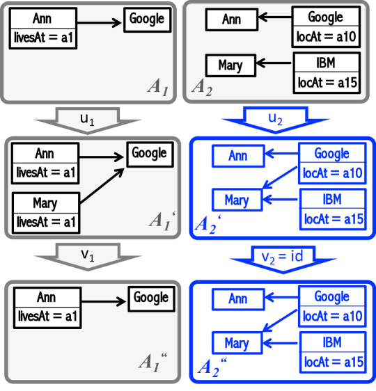
Figure 6: Unconstrained Putput is violated - Example 1

Figure 6 presents a simple example (we use a more compact notation, in which values of the attribute $\mathsf{name}$ are used as OIDs – the primary key attribute idea). At the initial moment, the binary multimodel $({A_{1}},{A_{2}})$ with the (implicit) corr given by name matching is consistent: the only intermodel constraint (C1) is satisfied. Update $u_{1}$ adds a new employment record to model $A_{1}$, constraint (C1) is violated, and to restore consistency, a new employment is added to $A_{2}$ by update $u_{2}=\mathsf{ppg}^{R}_{12}(u_{1})$ (the new propagated model and update are shown with blue lines and blank). Then update $v_{1}$ deletes the record added by $u_{1}$, but as the resulting multimodel $(A^{\prime\prime}_{1},A^{\prime}_{2})$ remains consistent, nothing should be done (if we follow the Hippocraticness principle in bx introduced by Stevens [31]) and thus $v_{1}$ is propagated to identity, $v_{2}=\mathsf{ppg}^{R^{\prime\prime}}_{12}(v_{1})=\mathsf{id}_{A^{\prime}_{2}}$. Now we notice that the composition $(u_{1};v_{1})$ is identity, and hence is to be propagated to identity, i.e., $\mathsf{ppg}^{R}_{12}(u_{1};v_{1})=\mathsf{id}_{A_{2}}$, while $\mathsf{ppg}^{R}_{12}(u_{1});\mathsf{ppg}^{R^{\prime\prime}}_{12}(v_{1})=u_{2};v_{2}=u_{2}\neq\mathsf{id}_{A_{2}}$, and $A^{\prime\prime}_{1}\neq A^{\prime\prime}_{2}$.

Obviously, the violation story will still hold if models $A_{1}$ and $A_{2}$ are much bigger and updates $u_{1}$ and $v_{1}$ are parts of bigger updates (but Mary should not appear in $A_{1}$).

Figure 7: Unconstrained Putput is violated–Example 2

Figure 7 presents a more interesting ternary example. Multi-model ${\cal A}$ is consistent, but update $u_{3}$ deletes route #1 and violates constraint (C2). In this case, the most direct propagation policy would delete all employment records related to #1 but, to keep changes minimal, would keep people in $A_{1}$ and companies in $A_{2}$ as specified by model ${\cal A}^{\prime}$ in the figure. Then a new route is inserted by update $v_{3}$ (note the new OID), which has the same $\mathsf{from}$ and $\mathsf{to}$ attributes as route #1. There are multiple ways to propagate such an insertion. The simplest one is to do nothing as the multimodel $(A^{\prime}_{1},A^{\prime}_{2},A^{\prime\prime}_{3},R^{\prime}=\varnothing)$ is consistent (recall that mapping $\mathsf{(e2r)}$ is not necessarily surjective). However, we can assume a more intelligent (non-Hippocratic) policy that looks for people with address a1 in the first database (and finds John and Mary), then checks somehow (e.g., by other attributes in the database schema $M_{1}$ which we did not show) if some of them are recent graduates in IT (and, for example, finds that Mary is such) and thus could work for a company at the address a10 (Google). Then such a policy would propagate update $v_{3}$ to $v_{1}$ and $v_{2}$ as shown in the figure. Now we notice that the composition of updates $u_{3}$ and $v_{3}$ is an identity, and thus $u_{3};v_{3}$ would be propagated to the identity on the multimodel ${\cal A}$. However, ${\cal A}^{\prime\prime}\neq{\cal A}$ and Putput fails. (Note that it would also fail if we used a simpler policy of propagating update $v_{3}$ to identity updates on $A^{\prime}_{1}$ and $A^{\prime}_{2}$.)

A common feature of the two examples is that the second update $v$ fully reverts the effect of the first one, $u$, while their propagations do not fully enjoy such a property due to some “side effects”. In fact, Putput is violated if update $v$ would just partially revert update $u$. Several other examples and a more general discussion of this phenomenon that forces Putput to fail can be found in [5]. However, it makes sense to require compositional update propagation for two sequentially compatible updates in the sense of Def. 1; we call the respective version of the law KPutput law with ’K’ recalling the sequential compatibility relation $\mathsf{K}^{{\blacktriangleright\!\!\blacktriangleright}}$. To manage update amendments, we will also need to use update merging operator $\mathsf{merge}$ as shown in Fig. 8

Definition 9 (Very well-behaved lenses)

A wb lens is called very well behaved (vwb), if it satisfies the following KPutput law for any $i$, corr $R\in\mathsf{corr}{A_{i}}$, and updates $u_{i}{:}\;A_{i}\rightarrow A^{\prime}_{i}$, $v_{i}{:}\;A^{\prime}_{i}\rightarrow B_{i}$ (see Fig. 8).

Let $u_{i}^{@}=\mathsf{ppg}^{R}_{ii}(u_{i})$. Suppose that $(u_{i},v_{i})\in\mathsf{K}^{{\blacktriangleright\!\!\blacktriangleright}}_{A_{i}^{\prime}}$ and $(v_{i},u_{i}^{@})\in\mathsf{K}^{{\blacktriangle{}}}_{A_{i}^{\prime}}$, then the merge $(\tilde{v}_{i},\widetilde{u_{i}^{@}})=\mathsf{merge}(v_{i},u_{i}^{@})$ is defined (see Fig. 8) and the following equalities are required to hold:
$\mathsf{{(\textsf{{KPutput}})}}_{j\neq i}$ $\mathsf{ppg}^{R}_{ij}(u_{i};v_{i})=\mathsf{ppg}^{R}_{ij}(u_{i});\mathsf{ppg}^{R^{\prime\prime}}_{ij}(\widetilde{v_{i}})$, and $(\mathsf{ppg}^{R}_{ij}(u_{i}),\mathsf{ppg}^{R^{\prime\prime}}_{ij}(\widetilde{v_{i}}))\in\mathsf{K}^{{\blacktriangleright\!\!\blacktriangleright}}_{A_{j}^{\prime\prime}}$, $\mathsf{{(\textsf{{KPutput}})}}_{ii}$ $(u_{i};v_{i})^{@}=\widetilde{u_{i}^{@}};(\widetilde{v_{i}})^{@}$
see the dashed arrows in Fig. 8, which depict the propagation of the composed updates. ∎

Figure 8: $\mathsf{{(\textsf{{KPutput}})}}$-Law (for update $x$, expression $x^{@}$ stands for the amendment $\mathsf{ppg}^{R(x)}_{ii}(x)$ with $R(x)$ being the corr at the source of $x$ – it labels the corresponding horizontal dotted line)

Corollary 1 (Closed vwb lenses)

For a vwb lens as defined above, if update $u_{i}$ is $R$-closed (i.e., $u_{i}^{@}=\mathsf{id}_{A^{\prime}}$), then the following equations hold:

$\mathsf{{(\textsf{{KPutput}})}}_{j\neq i}^{\mathsf{closed}}$	$\mathsf{ppg}^{R}_{ij}(u_{i};v_{i})=\mathsf{ppg}^{R}_{ij}(u_{i});\mathsf{ppg}^{R^{\prime\prime}}_{ij}({v_{i}})$,
	and $(\mathsf{ppg}^{R}_{ij}(u_{i}),\mathsf{ppg}^{R^{\prime\prime}}_{ij}({v_{i}}))\in\mathsf{K}^{{\blacktriangleright\!\!\blacktriangleright}}_{A_{j}^{\prime\prime}}$,
$\mathsf{{(\textsf{{KPutput}})}}_{ii}^{\mathsf{closed}}$	$(u_{i};v_{i})^{@}=v_{i}^{@}$

6 Compositionality of Model Synchronization: Playing Lego with Lenses

We study how lenses can be composed. Assembling well-behaved and well-tested small components into a bigger one is a cornerstone of software engineering. If a mathematical theorem guarantees that desired properties carry over from the components to the composition, additional integration tests for checking these properties are no longer necessary. This makes lens composition results practically important.

In Sect. 6.1, we consider parallel composition of lenses, which is easily manageable. Sequential composition, in which different lenses share some of their feet, and updates propagated by one lens are taken and propagated further by one or several other lenses, is much more challenging and considered in the other two subsections. In Sect. LABEL:sec:lego-star, we consider ”star-composition”, cf. Fig. LABEL:fig:starComposition and show that under certain additional assumptions (very) well-behavedness carries over from the components to the composition. However, invertibility does not carry over to the composition – we shows this with a counterexample in Sect. LABEL:sec:invert. In Sect. LABEL:sec:lego-spans2lens, we study how (symmetric) lenses can be assembled from asymmetric ones and prove two easy theorems on the property preservation for such composition.

Since we now work with several lenses, we need a notation for lens’ components. Given a lens $\ell=({\boldsymbol{\mathcal{A}}},\mathsf{ppg})$, we write $\mathbf{A}^{\ell},\mathbf{A}(\ell)$ or $\boldsymbol{\partial}\ell$ for $\boldsymbol{\partial}{\boldsymbol{\mathcal{A}}}$, $\mathsf{Corr}^{\ell}$ or $\mathsf{Corr}(\ell)$ for $\mathsf{Corr}({\boldsymbol{\mathcal{A}}})$, and $\partial^{\ell}_{i}(R)$ for the $i$-th boundary of corr $R$. Propagation operations of the lens $\ell$ are denoted by $\ell.\mathsf{ppg}_{ij}^{R}$, $\ell.\mathsf{ppg}_{i\star}^{R}$. We will often identify an aligned multimodel $(A,R)$ and its corr $R$ as they are mutually derivable (see Remark 1 on p.1).

We will also need the notion of lens isomorphism.

Definition 10 (Isomorphic lenses)

Two $n$-ary lenses $\ell$ and $\ell^{\prime}$ are isomorphic, $\ell\cong\ell^{\prime}$, if
(a) their feet are isomorphic via a family of isomorphism functors $f_{i}{:}\;\mathbf{A}^{\ell}_{i}\rightarrow\mathbf{A}^{\ell^{\prime}}_{i}$;
(b) their classes of corrs are isomorphic via bijection $f_{\mathsf{Corr}}{:}\;\mathsf{Corr}^{\ell}\rightarrow\mathsf{Corr}^{\ell^{\prime}}$ commuting with boundaries: $\partial^{\ell^{\prime}}_{i}(f_{\mathsf{Corr}}(R))=f_{i}(\partial^{\ell}_{i}(R))$ for all $i$;
(c) their propagation operations are compatible with isomorphisms above: for any foot update $u_{i}{:}\;A_{i}^{\ell}\rightarrow B_{i}^{\ell}$ and corr $R\in\mathsf{Corr}^{\ell}(A_{i})$ for lens $\ell$, we have

$$f_{j}(\ell.\mathsf{ppg}^{R}_{ij}(u_{i}))=\ell^{\prime}.\mathsf{ppg}^{f_{\mathsf{Corr}}(R)}_{ij}(f_{i}(u_{i})).$$

That is, two composed mappings, one propagates $u_{i}$ with lens $\ell$ then maps the result to $\ell^{\prime}$-space, and the other maps $u_{i}$ to $\ell^{\prime}$-space and then propagates it with lens $\ell^{\prime}$, produce the same result.

6.1 Parallel Lego: Lenses working in parallel

We will consider two types of parallel composition. The first is chaotic (co-discrete in the categorical parlance). Suppose we have several clusters of synchronized models, i.e., models within the same cluster are synchronized but models in different clusters are independent. We can model such situations by considering several lenses $\ell_{1},...,\ell_{k}$, each one working over its own multimodel space ${\boldsymbol{\mathcal{A}}}_{i}$. Although mutually independent w.r.t data, clusters are time-related and it makes sense to talk about multimodels ${\cal A}_{1}^{t},...,{\cal A}_{k}^{t}$ coexisting at some time moment $t$: such a tuple of multimodels can be seen as the state of the multi-multimodel ${\cal A}_{1}\times\ldots\times{\cal A}_{k}$ at moment $t$. As model clusters are data-independent, we can propagate tuples of updates $(u_{1},\ldots,u_{k})$ — one update per cluster, to other such tuples. For example, if we have a ternary lens $\mathpzc{k}$ with feet $\mathbf{A}_{i}$, $i=1..3$, and a binary lens $\ell$ with feet $\mathbf{B}_{j}$, $j=1,2$, any pair of updates $(u_{i},v_{j})\in\mathbf{A}_{i}{\times}\mathbf{B}_{j}$ can be propagated to pairs $(u_{i^{\prime}},v_{j^{\prime}})\in\mathbf{A}_{i^{\prime}}{\times}\mathbf{B}_{j^{\prime}}$ with $i^{\prime}=1..3$ and $j^{\prime}=1,2$ by the two lenses working in parallel: lens $\mathpzc{k}$ propagates $u_{i}$ and $\ell$ propagates $v_{j}$. The resulting synchronization can be seen as a six-ary lens with feet $\mathbf{A}_{i}\times\mathbf{B}_{j}$. A general construction that composes lenses $\ell_{1},\ldots,\ell_{k}$ of arities $n_{1},\ldots,n_{k}$ resp., into a product lens $\ell_{1}\times\ldots\times\ell_{k}$ of arity $n_{1}\times n_{2}\times...\times n_{k}$ is described in Sect. 6.1.1

Our second construct of parallel composition is for lenses of the same arity working in a strongly coordinated way. Suppose that our traffic agency has several branches in different cities, all structured in a similar way, i.e., over metamodels $M_{i}$, $i=1,2,3$ in Fig. 2. However, now we have families of models $A^{x}_{i}$ with $x$ ranging over cities. Suppose also a strong discipline of coordinated updates, in which all models of the same type, i.e., with a fixed metamodel index $i$ but different city index $x$, are updated simultaneously. Then global updates are tuples like $\left(\mathstrut{u^{x}_{1}{:}\;A^{x}_{1}\rightarrow A^{\prime x}_{1}}\,|\;{x\in\mathrm{Cities}}\right)$ or $\left(\mathstrut{u^{x}_{2}{:}\;A^{x}_{2}\rightarrow A^{\prime x}_{2}}\,|\;{x\in\mathrm{Cities}}\right)$. Such tuples can be propagated componentwise, i.e., city-wise, so that we have a global ternary lens, whose each foot is indexed by cities. Thus, in contrast to the chaotic parallel composition, the arity of the coordinated composed lens equals to the arity of components. We will formally define the construct in Sect. 6.1.2.

6.1.1 6.1.1. Chaotic Parallel Composition.

Definition 11

Let $\mathpzc{k}$ and $\ell$ be two lenses of arities $m$ and $n$. We first choose the following two-dimensional enumeration of their product $mn$: any number $1\leq i\leq mn$ is assigned with two natural numbers as specified below:

(2) $$i\mapsto({i{k}},{i_{\ell}})=\begin{cases}(1,i)\text{ if }1\leq i\leq n,\\ (2,i)\text{ if }n<i\leq 2n,\\ \ldots\\ (m,i)\text{ if }(m{-}1)n<i\leq mn,\end{cases}$$

Of course, we could choose another such enumeration but its only effect is reindexing/renaming the feet while synchronization as such is not affected. Now we define the chaotic parallel composition of $\mathpzc{k}$ and $\ell$ as the $m{\times}n$-ary lens $\mathpzc{k}{\times}\ell$ with Boundary spaces: $\boldsymbol{\partial}_{i}^{\mathpzc{k}{\times}\ell}=(\boldsymbol{\partial}{k}_{i{k}},\boldsymbol{\partial}^{\ell}_{i_{\ell}})$ Corrs: $\mathsf{Corr}(\mathpzc{k}{\times}\ell)=\mathsf{Corr}(\mathpzc{k})\times\mathsf{Corr}(\ell)$ with boundaries $\partial_{i}^{(\mathpzc{k}{\times}\ell)}(Q,R)=(\partial_{i{k}}{k}(Q),\partial_{i_{\ell}}^{\ell}(R))$ for all $i$ Operations: Given an update $\mathbf{u}_{i}$ at foot $i$ of lens $\mathpzc{k}{\times}\ell$, i.e., a pair of updates $(u_{i{k}},v_{i_{\ell}})$ with $u_{i{k}}{:}\;A_{i{k}}\rightarrow A^{\prime}_{i{k}}$, $v_{i_{\ell}}{:}\;B_{i_{\ell}}\rightarrow B^{\prime}_{i_{\ell}}$, and corrs $Q\in\mathsf{Corr}{k}(A_{{i{k}}})$, $R\in\mathsf{Corr}^{\ell}(B_{{i_{\ell}}})$, we define $(\mathpzc{k}{\times}\ell).\mathsf{ppg}_{ij}^{(Q,R)}(\mathbf{u}_{i})\stackrel{{\scriptstyle\mathrm{def}}}{{=}}(\mathpzc{k}.\mathsf{ppg}_{{i{k}}{j{k}}}^{Q}(u_{i{k}}),\,\ell.\mathsf{ppg}_{{i_{\ell}}{j_{\ell}}}^{R}(v_{i_{\ell}}))$ $(\mathpzc{k}{\times}\ell).\mathsf{ppg}_{i\star}^{(Q,R)}(\mathbf{u}_{i})\stackrel{{\scriptstyle\mathrm{def}}}{{=}}(\mathpzc{k}.\mathsf{ppg}_{{i{k}}\star}^{Q}(u_{i{k}}),\,\ell.\mathsf{ppg}_{{i_{\ell}}\star}^{Q}(v_{i_{\ell}})).$ Furthermore, for any models $A\in\mathsf{Ob}(\mathbf{A})$ and $B\in\mathsf{Ob}(\mathbf{B})$, relations $\mathsf{K}^{{\blacktriangleright\!\!\blacktriangleright}}_{\!A\times B}$ and $\mathsf{K}^{{\blacktriangle{}}}_{A\times B}$ are the obvious rearrangement of elements of $\mathsf{K}^{{\blacktriangleright\!\!\blacktriangleright}}_{A}\times\mathsf{K}^{{\blacktriangleright\!\!\blacktriangleright}}_{B}$ and $\mathsf{K}^{{\blacktriangle{}}}_{A}\times\mathsf{K}^{{\blacktriangle{}}}_{B}$. ∎

Lemma 1

If $\mathpzc{k}$ and $\ell$ are (very) wb (and invertible), then $\mathpzc{k}{\times}\ell$ is (very) wb (and invertible).

Proof

All verifications can be carried out componentwise.∎

Lemma 2

Chaotic parallel composition is associative up to isomorphism: $(\mathpzc{k}\times\ell)\times\ell^{\prime}\cong\mathpzc{k}\times(\ell\times\ell^{\prime})$

Another important difference is update amendments, which are not considered in [32] – models in the authority set are intact. Yet another distinction is how the multiary vs. binary issue is treated. Stevens provides several results for decomposing an n-ary relation $R\in\mathsf{Corr}(\mathbf{A})$ into binary relations $R_{ij}\subseteq\mathsf{Ob}(\mathbf{A}_{i}){\times}\mathsf{Ob}(\mathbf{A}_{j})$ between the components. For us, a relation is inherently $n$-ary, i.e., a set $R$ of $n$-ary links endowed with an $n$-tuple of projections $\partial_{i}{:}\;R\rightarrow A_{i}$ uniquely identifying links’ boundaries. Thus, while Stevens considers “binarization” of a relation $R$ by a chain of binary relations over the “perimeter” $A_{1}...A_{n}$, we binarize it via the corresponding span of (binary) mappings $(\partial_{1},{...},\partial_{n})$ (UML could call this process reification). Our (de)composition results demonstrate advantages of the span view.

Discussion of several other works in the state-based world, notably by Macedo et al [27] can be found in [32]. Several remarks about the related work on the Putput law have already been made in Sect. 2.3

9 Conclusion

Multimodel synchronization is an important practical problem, which cannot be fully automated but even partial automation would be beneficial. A major problem in building an automatic support is uncertainty inherent to consistency restoration. In this regard, restoration via update propagation rather than immediate repairing of an inconsistent state of the multimodel has an essential advantage: having the update causing inconsistency as an input for the restoration operation can guide the propagation policy and essentially reduce the uncertainty. We thus come to the scenario of multiple model synchronization via multi-directional update propagation. We have also argued that reflective propagation to the model whose change originated inconsistency is a reasonable feature of the scenario.

We presented a mathematical framework for synchronization scenarios as above based on a multiary generalization of binary symmetric delta lenses introduced earlier, and enriched it with reflective propagation and KPutput law ensuring compatibility of update propagation with update composition in a practically reasonable way (in contrast to the strong but unrealistic Putput). We have also defined several operations of composing multiary lenses in parallel and sequentially. Our lens composition results make the framework  interesting for practical applications: if a tool builder has implemented a library of elementary synchronization modules based on lenses and, hence, ensuring basic laws for change propagation, then a complex module assembled from elementary lenses will automatically be a lens and thus also enjoys the basic laws. This allows one to avoid additional integration testing, which can essentially reduce the cost of synchronization software.

Acknowledgement. We are really grateful to anonymous reviewers for careful reading of the manuscript and detailed, pointed, and stimulating reviews, which essentially improved the presentation and discussion of the framework.

References

- [1] Bohannon, A., Foster, J.N., Pierce, B.C., Pilkiewicz, A., Schmitt, A.: Boomerang: resourceful lenses for string data. In: Necula, G.C., Wadler, P. (eds.) POPL. pp. 407–419. ACM (2008)
- [2] Chechik, M., Nejati, S., Sabetzadeh, M.: A relationship-based approach to model integration. ISSE 8(1), 3–18 (2012), https://doi.org/10.1007/s11334-011-0155-2
- [3] Demuth, A., Riedl-Ehrenleitner, M., Nöhrer, A., Hehenberger, P., Zeman, K., Egyed, A.: Designspace: an infrastructure for multi-user/multi-tool engineering. In: Wainwright, R.L., Corchado, J.M., Bechini, A., Hong, J. (eds.) Proceedings of the 30th Annual ACM Symposium on Applied Computing, Salamanca, Spain, April 13-17, 2015. pp. 1486–1491. ACM (2015), https://doi.org/10.1145/2695664.2695697
- [4] Diskin, Z.: Model Synchronization: Mappings, Tiles, and Categories. In: Fernandes, J.M., Lämmel, R., Visser, J., Saraiva, J. (eds.) GTTSE. Lecture Notes in Computer Science, vol. 6491, pp. 92–165. Springer (2011)
- [5] Diskin, Z.: Compositionality of update propagation: Lax putput. In: Eramo, R., Johnson, M. (eds.) Proceedings of the 6th International Workshop on Bidirectional Transformations co-located with The European Joint Conferences on Theory and Practice of Software, BX@ETAPS 2017, Uppsala, Sweden, April 29, 2017. CEUR Workshop Proceedings, vol. 1827, pp. 74–89. CEUR-WS.org (2017), http://ceur-ws.org/Vol-1827/paper12.pdf
- [6] Diskin, Z., Gholizadeh, H., Wider, A., Czarnecki, K.: A three-dimensional taxonomy for bidirectional model synchronization. Journal of System and Software 111, 298–322 (2016), https://doi.org/10.1016/j.jss.2015.06.003
- [7] Diskin, Z., König, H., Lawford, M.: Multiple model synchronization with multiary delta lenses. In: Russo, A., Schürr, A. (eds.) Fundamental Approaches to Software Engineering, 2018. Lecture Notes in Computer Science, vol. 10802, pp. 21–37. Springer (2018), https://doi.org/10.1007/978-3-319-89363-1_2
- [8] Diskin, Z., König, H., Lawford, M., Maibaum, T.: Toward product lines of mathematical models for software model management. In: Seidl, M., Zschaler, S. (eds.) Software Technologies: Applications and Foundations - STAF 2017 Collocated Workshops, Marburg, Germany, July 17-21, 2017, Revised Selected Papers. Lecture Notes in Computer Science, vol. 10748, pp. 200–216. Springer (2017), https://doi.org/10.1007/978-3-319-74730-9_19
- [9] Diskin, Z., Xiong, Y., Czarnecki, K.: Specifying Overlaps of Heterogeneous Models for Global Consistency Checking. In: MoDELS Workshops. LNCS, vol. 6627, pp. 165–179. Springer (2010)
- [10] Diskin, Z., Xiong, Y., Czarnecki, K.: From State- to Delta-Based Bidirectional Model Transformations: the Asymmetric Case. Journal of Object Technology 10, 6: 1–25 (2011)
- [11] Diskin, Z., Xiong, Y., Czarnecki, K., Ehrig, H., Hermann, F., Orejas, F.: From state-to delta-based bidirectional model transformations: the symmetric case. In: MODELS, pp. 304–318. Springer (2011)
- [12] Ehrig, H., Ehrig, K., Prange, U., Taenzer, G.: Fundamentals of Algebraic Graph Transformation (2006)
- [13] Ehrig, H., Ehrig, K., U.Prange, Taentzer, G.: Fundamentals of algebraic graph tranformations. Springer (2006)
- [14] Foster, J.N., Greenwald, M.B., Moore, J.T., Pierce, B.C., Schmitt, A.: Combinators for bi-directional tree transformations: a linguistic approach to the view update problem. In: Palsberg, J., Abadi, M. (eds.) Proceedings of the 32nd ACM SIGPLAN-SIGACT Symposium on Principles of Programming Languages, POPL 2005, Long Beach, California, USA, January 12-14, 2005. pp. 233–246. ACM (2005), http://doi.acm.org/10.1145/1040305.1040325
- [15] Foster, J.N., Greenwald, M.B., Moore, J.T., Pierce, B.C., Schmitt, A.: Combinators for bidirectional tree transformations: A linguistic approach to the view-update problem. ACM Transactions on Programming Languages and Systems (TOPLAS) 29(3), 17 (2007)
- [16] Hermann, F., Ehrig, H., Ermel, C., Orejas, F.: Concurrent model synchronization with conflict resolution based on triple graph grammars. Fundamental Approaches to Software Engineering pp. 178–193 (2012)
- [17] Hermann, F., Ehrig, H., Orejas, F., Czarnecki, K., Diskin, Z., Xiong, Y.: Correctness of model synchronization based on triple graph grammars. In: MODELS, pp. 668–682. Springer (2011)
- [18] Hofmann, M., Pierce, B.C., Wagner, D.: Symmetric lenses. In: Ball, T., Sagiv, M. (eds.) Proceedings of the 38th ACM SIGPLAN-SIGACT Symposium on Principles of Programming Languages, POPL 2011, Austin, TX, USA, January 26-28, 2011. pp. 371–384. ACM (2011), http://doi.acm.org/10.1145/1926385.1926428
- [19] Hofmann, M., Pierce, B.C., Wagner, D.: Edit lenses. In: Field, J., Hicks, M. (eds.) Proceedings of the 39th ACM SIGPLAN-SIGACT Symposium on Principles of Programming Languages, POPL 2012, Philadelphia, Pennsylvania, USA, January 22-28, 2012. pp. 495–508. ACM (2012), http://doi.acm.org/10.1145/2103656.2103715
- [20] Johnson, M., Rosebrugh, R.D.: Lens put-put laws: monotonic and mixed. ECEASST 49 (2012)
- [21] Johnson, M., Rosebrugh, R.D.: Unifying set-based, delta-based and edit-based lenses. In: Anjorin, A., Gibbons, J. (eds.) Proceedings of the 5th International Workshop on Bidirectional Transformations, Bx 2016, co-located with The European Joint Conferences on Theory and Practice of Software, ETAPS 2016, Eindhoven, The Netherlands, April 8, 2016. CEUR Workshop Proceedings, vol. 1571, pp. 1–13. CEUR-WS.org (2016), http://ceur-ws.org/Vol-1571/paper_13.pdf
- [22] Johnson, M., Rosebrugh, R.D.: Symmetric delta lenses and spans of asymmetric delta lenses. Journal of Object Technology 16(1), 2:1–32 (2017), https://doi.org/10.5381/jot.2017.16.1.a2
- [23] Johnson, M., Rosebrugh, R.D.: Cospans and symmetric lenses. In: Conference Companion of the 2nd International Conference on Art, Science, and Engineering of Programming, Nice, France, April 09-12, 2018. pp. 21–29 (2018), http://doi.acm.org/10.1145/3191697.3191717
- [24] Johnson, M., Rosebrugh, R.D., Wood, R.J.: Lenses, fibrations and universal translations. Mathematical Structures in Computer Science 22(1), 25–42 (2012), https://doi.org/10.1017/S0960129511000442
- [25] Knapp, A., Mossakowski, T.: Multi-view consistency in UML. CoRR abs/1610.03960 (2016), http://arxiv.org/abs/1610.03960
- [26] König, H., Diskin, Z.: Efficient consistency checking of interrelated models. In: Modelling Foundations and Applications - 13th European Conference, ECMFA 2017, Held as Part of STAF 2017, Marburg, Germany, July 19-20, 2017, Proceedings. pp. 161–178 (2017), https://doi.org/10.1007/978-3-319-61482-3_10
- [27] Macedo, N., Cunha, A., Pacheco, H.: Towards a framework for multidirectional model transformations. In: Proceedings of the Workshops of the EDBT/ICDT 2014 Joint Conference (EDBT/ICDT 2014), Athens, Greece, March 28, 2014. pp. 71–74 (2014), http://ceur-ws.org/Vol-1133/paper-11.pdf
- [28] Marussy, K., Semeráth, O., Varró, D.: Incremental view model synchronization using partial models. In: Wasowski, A., Paige, R.F., Haugen, Ø. (eds.) Proceedings of the 21th ACM/IEEE International Conference on Model Driven Engineering Languages and Systems, MODELS 2018, Copenhagen, Denmark, October 14-19, 2018. pp. 323–333. ACM (2018), https://doi.org/10.1145/3239372.3239412
- [29] Orejas, F., Boronat, A., Ehrig, H., Hermann, F., Schölzel, H.: On propagation-based concurrent model synchronization. ECEASST 57 (2013), http://journal.ub.tu-berlin.de/eceasst/article/view/871
- [30] Rabbi, F., Lamo, Y., Yu, I.C., Kristensen, L.M.: A diagrammatic approach to model completion. In: Proceedings of the 4th Workshop on the Analysis of Model Transformations co-located with the 18th International Conference on Model Driven Engineering Languages and Systems (MODELS 2015), Ottawa, Canada, September 28, 2015. pp. 56–65 (2015), http://ceur-ws.org/Vol-1500/paper7.pdf
- [31] Stevens, P.: Bidirectional model transformations in qvt: semantic issues and open questions. Software & Systems Modeling 9(1), 7–20 (2010)
- [32] Stevens, P.: Bidirectional transformations in the large. In: 20th ACM/IEEE International Conference on Model Driven Engineering Languages and Systems, MODELS 2017, Austin, TX, USA, September 17-22, 2017. pp. 1–11 (2017), https://doi.org/10.1109/MODELS.2017.8
- [33] Trollmann, F., Albayrak, S.: Extending model to model transformation results from triple graph grammars to multiple models. In: Theory and Practice of Model Transformations - 8th International Conference, ICMT 2015, Held as Part of STAF 2015, L’Aquila, Italy, July 20-21, 2015. Proceedings. pp. 214–229 (2015), https://doi.org/10.1007/978-3-319-21155-8_16
- [34] Trollmann, F., Albayrak, S.: Extending model synchronization results from triple graph grammars to multiple models. In: Theory and Practice of Model Transformations - 9th International Conference, ICMT 2016, Held as Part of STAF 2016, Vienna, Austria, July 4-5, 2016, Proceedings. pp. 91–106 (2016), https://doi.org/10.1007/978-3-319-42064-6_7
- [35] Trollmann, F., Albayrak, S.: Decision points for non-determinism in concurrent model synchronization with triple graph grammars. In: Theory and Practice of Model Transformation - 10th International Conference, ICMT 2017, Held as Part of STAF 2017, Marburg, Germany, July 17-18, 2017, Proceedings. pp. 35–50 (2017), https://doi.org/10.1007/978-3-319-61473-1_3