Ion-acoustic rogue waves in a multi-component plasma medium

Abstract

The nonlinear propagation of ion-acoustic (IA) waves (IAWs) in a four component plasma medium (FCPM) containing inertial warm positive ions, and inertialess iso-thermal cold electrons as well as non-extensive ($q$-distributed) hot electrons and positrons is theoretically investigated. A nonlinear Schrödinger equation (NLSE) is derived by using the reductive perturbation method, and it is observed that the FCPM under consideration supports both modulationally stable and unstable parametric regimes which are determined by the sign of the dispersive and nonlinear coefficients of NLSE. The numerical analysis has shown that the maximum value of the growth rate decreases with the increase in $q$ ($q>1$), and the modulationally unstable parametric regime allows to generate highly energetic IA rogue waves (IARWs), and the amplitude and width of the IARWs increase with an increase in the value of hot electron number density while decrease with an increase in the value of cold electron number density. The applications of our investigation in understanding the basic features of nonlinear electrostatic perturbations in many space plasma environments and laboratory devices are briefly discussed.

1 Introduction

The existence of the electron-positron-ion (EPI) plasma has been identified in astrophysical environments such as Saturn’s magnetosphere [1, 2, 3, 4, 5, 6], pulsar magnetosphere, active galactic nuclei, early universe [1], neutron stars, Sun atmosphere [1], and has also been confirmed in various laboratory experiments such as intense laser field. The formation and propagation of various kinds of electrostatic waves namely, ion-acoustic (IA) waves (IAWs) [1, 2, 3, 4, 5, 6, 7], electron-acoustic waves (EAWs) [8], and positron-acoustic waves (PAWs) as well as their associated nonlinear structures (viz., solitons, double layers, shocks, and vortices, etc.) in space and laboratory EPI plasma have been significantly modified by the presence of positrons.

The co-existence of hot and cold electrons in Saturn’s magnetosphere has been identified by the Voyager PLS observations [9, 10, 11] and the CAPS (Cassini Plasma Spectrometer) observations [12], and this identification has attracted a number of authors [1, 2, 3, 4, 5, 6, 7] to study the nonlinear properties of the plasma system having two temperature electrons. Rehman and Mishra [1] analytically and numerically analyzed the IA Gardner solitons in an EPI plasma with two temperature electrons. Shahmansouri and Alinejad [2] studied IA solitary waves in an three components plasma medium having inertialess cold and hot electrons as well as inertial ions, and reported that this model supports both compressive and rarefactive solitary structures in presence of two temperature electrons. Panwar et al. [4] considered three components plasma model having inertial positive ion and inertialess cold and hot electrons to study the propagation of nonlinear IA cnoidal waves, and found that the height and width of a cnoidal waves increase with the ratio of cold and hot electrons temperature. Baluku and Helberg [7] examined the nonlinear properties of the IA solitons in a plasma with two temperature electrons.

The deviation of the plasma species from the equilibrium state due to the activation of long range coulomb force field, wave-particle interaction, and other external force fields is described by the non-extensive $q$-distribution [3]. The parameter $q$ in $q$-distribution indicates the non-extensive properties of the plasma species in a non-equilibrium plasma system, and when $q$ is equal to unity then the $q$-distribution coincides with well-known Maxwellian distribution. When $q$ is less than one (i.e., $q<1$) then the plasma species indicate the super-extensive properties while $q$ is greater than one (i.e., $q>1$) then the plasma species indicate the sub-extensive properties [3].

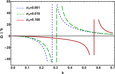
Figure 1: The variation of $P/Q$ with $k$ for different values of $\sigma_{h}$ when $\alpha$=$0.04$, $\gamma_{c}=0.5$, $\gamma_{h}=0.8$, $\sigma_{p}=0.01$, $q_{h}=1.3$, and $q_{p}=1.5$.

The standard nonlinear Schrödinger equation (NLSE) is the first platform to investigate the nonlinear properties of the dispersive plasma medium as well as the modulational instability (MI) of IAWs, EAWs, and PAWs as well as their associated first and second order rogue waves (RWs) in the dispersive plasma medium [13, 14, 15, 16, 17, 18, 19]. Shalini et al. [3] considered three component plasma model having inertialess two temperature electrons and inertial ions, and studied the MI of IAWs, and observed the effects of the non-extensivity of hot and cold electrons. Kourakis and Shukla [5] considered three component plasma model in presence of two temperature electron species, and demonstrated the MI of IAWs by deriving standard NLSE, and reported that a strong temperature difference between hot and cold electrons may favourable to bright envelope solitons. Alinejad et al. [6] studied the stability of the IAWs in a plasma medium having two temperature electrons. Therefore, in our present paper, we will study the MI of the IAWs and the mechanism of generating the first and second order IA RWs (IARWs) in a four component plasma medium (FCPM) having inertial warm ions, and inertialess iso-thermal cold electrons and non-extensive hot electrons and positrons.

The manuscript is organized as follows: The basic model equations are presented in Sec. 2. A NLSE is derived in Sec. 3. The MI and RWs are provided in Sec. 4. Results and discussion are presented in Sec. 5. Finally, a brief conclusion is given in Sec. 6.

2 Governing Equations

We consider a four component unmagnetized plasma model consisting of inertial warm ions, inertialess non-extensive hot electrons and positrons as well as iso-thermal cold electrons following Maxwellian distribution. At equilibrium, the overall charge neutrality condition for our plasma model can be written as $Z_{i}n_{i0}+n_{p0}=n_{c0}+n_{h0}$; where $n_{i0}$, $n_{p0}$, $n_{c0}$, and $n_{h0}$ are the equilibrium number densities of warm ions, non-extensive positrons, and cold and hot electrons, respectively, and $Z_{i}$ is the number of protons residing onto the ion surface. The normalized governing equations to study the IAWs are as follows:

$$\frac{\partial n_{i}}{\partial t}+\frac{\partial}{\partial x}(n_{i}u_{i})=0,$$ (1)

$$\frac{\partial u_{i}}{\partial t}+u_{i}\frac{\partial u_{i}}{\partial x}+\alpha n_{i}\frac{\partial n_{i}}{\partial x}=-\frac{\partial\phi}{\partial x},$$ (2)

$$\frac{\partial^{2}\phi}{\partial x^{2}}=\gamma_{c}n_{c}+\gamma_{h}n_{h}-(\gamma_{c}+\gamma_{h}-1)n_{p}-n_{i},\$$ (3)

where $n_{i}$ is the number density of inertial warm ions normalized by its equilibrium value $n_{i0}$; $u_{i}$ is the ion fluid speed normalized by the IAW speed $C_{i}=(Z_{i}k_{B}T_{c}/m_{i})^{1/2}$ (with $T_{c}$ being the $q$-distributed cold electron temperature, $m_{i}$ being the ion rest mass, and $k_{B}$ being the Boltzmann constant); $\phi$ is the electrostatic wave potential normalized by $k_{B}T_{c}/e$ (with $e$ being the magnitude of single electron charge); the time and space variables are normalized by ${\omega^{-1}_{pi}}=(m_{i}/4\pi Z^{2}e^{2}n_{i0})^{1/2}$ and $\lambda_{Di}=(k_{B}T_{c}/4\pi Ze^{2}n_{i0})^{1/2}$, respectively. The pressure term of the ion can be written as $p_{i}=p_{i0}(N_{i}/n_{i0})^{\gamma}$ with $p_{i0}=n_{i0}k_{B}T_{i}$ being the equilibrium pressure of the ion, and $T_{i}$ being the temperature of warm ion, and $\gamma=(N+2)/N$ (where $N$ is the degrees of freedom and for one-dimensional case $N=1$ then $\gamma=3$). Other parameters are defined as $\alpha=3T_{i}/Z_{i}T_{c}$, $\gamma_{c}=n_{c0}/Z_{i}n_{i0}$, and $\gamma_{h}=n_{h0}/Z_{i}n_{i0}$. The expression for the number density of cold electrons following the Maxwellian distribution can be expressed as

$$n_{c}=\mbox{exp}(\phi)=1+\phi+\frac{\phi^{2}}{2}+\frac{\phi^{3}}{6}+\cdot\cdot\cdot,\$$ (4)

Now, the expressions for the number density of hot electrons following the $q$-distribution can be expressed as [15]

$$n_{h}=[1+(q_{h}-1)\sigma_{h}\phi]^{\frac{(q_{h}+1)}{2(q_{h}-1)}}=1+A_{1}\phi+A_{2}\phi^{2}+A_{3}\phi^{3}+\cdot\cdot\cdot,\$$ (5)

where $q_{h}$ is the non-extensivity of the hot electrons, $\sigma_{h}$ = ${T_{c}}/{T_{h}}$ (with $T_{h}$ being the $q$-distributed hot electron temperature), and

$$A_{1}=[(q_{h}+1)\sigma_{h}]/2,~{}~{}~{}A_{2}=[(q_{h}+1)(3-q_{h})\sigma_{h}^{2}]/8,~{}~{}~{}A_{3}=[(q_{h}+1)(3-q_{h})(5-3q_{h})\sigma_{h}^{3}]/48.\$$

Now, the expressions for the number density of hot positrons following the $q$-distribution can be expressed as [15]

$$n_{p}=[1-(q_{p}-1)\sigma_{p}\phi]^{\frac{(q_{p}+1)}{2(q_{p}-1)}}=1-A_{4}\phi+A_{5}\phi^{2}-A_{6}\phi^{3}+\cdot\cdot\cdot,\$$ (6)

where $q_{p}$ is the non-extensivity of the positrons, $\sigma_{p}$ = ${T_{c}}/{T_{p}}$ (with $T_{p}$ being the $q$-distributed positron temperature), and

$$A_{4}=[(q_{p}+1)\sigma_{p}]/2,~{}~{}~{}A_{5}=[(q_{p}+1)(3-q_{p})\sigma_{p}^{2}]/8,~{}~{}~{}A_{6}=[(q_{p}+1)(3-q_{p})(5-3q_{p})\sigma_{p}^{3}]/48.\$$

The parameter $q_{h}$ and $q_{p}$ are generally known as entropic index. Now, by substituting Eqs. (4)-(6) into Eq. (3) and expanding up to third order of $\phi$, we get

$$\frac{\partial^{2}\phi}{\partial x^{2}}+n_{i}=1+A_{7}\phi+A_{8}\phi^{2}+A_{9}\phi^{3}+\cdot\cdot\cdot,$$ (7)

where

$$A_{7}=\gamma_{c}+\gamma_{h}A_{1}+(\gamma_{c}+\gamma_{h}-1)A_{4},$$

$$A_{8}=[\gamma_{c}+{2\gamma_{h}A_{2}-2(\gamma_{c}+\gamma_{h}-1)A_{5}}]/2,$$

$$A_{9}=[\gamma_{c}+{6\gamma_{h}A_{3}+6(\gamma_{c}+\gamma_{h}-1)A_{6}}]/6.\$$

We note that Eq. (1), (2), and (7) now represent the basis set of normalized equations to describe the nonlinear dynamics of the IAWs, and associated IARWs in the FCPM under consideration. We also note that the works [13, 14, 15, 16, 17, 18, 19] may seem to be similar to our present investigation, but, in fact, they are not due to the following reasons:

• Ahmed et al. [13], Khondaker et al. [14], and Chowdhury et al. [15] studied the MI of IAWs, in which the moment of inertial is provided by the positive and negative ions and the restoring force is provided by the thermal pressure of the non-thermal (super-thermal $\kappa$-distributed and $q$-distributed) electrons and positrons in a pair-ion plasma medium, and observed the existence of the IARWs in the modulationally unstable parametric regimes. However, in our present work we have considered a FCPM consisting of inertial warm ions, $q$-distributed positrons, and non-inertial two temperatures electrons [say, hot electrons (following $q$-distribution), cold electrons (following Maxwellian distribution)]. We have examined the conditions of MI of the IAWs (where, the warm positive ions provides the moment of inertia and the thermal pressure of the positrons and two temperature electrons provides the restoring force).

• Rahman et al. [16] and Jahan et al. [17] investigated the stable and unstable parametric regimes of the dust-acoustic waves (DAWs) according to the sign of dispersive and nonlinear coefficients of the standard NLSE in a FCPM having inertial opposite polarity dust grains and inertialess non-thermal or iso-thermal ions as well as non-extensive electrons. Rahman et al. [18] analyzed theoretically and numerically the MI conditions of the DAWs in a FCPM having inertial cold and hot dust grains and inertialess non-extensive electrons and ions. But our present work is concerned with the MI of IAWs in presence of hot and cold electron species.

• Chowdhury et al. [19] studied the formation of only first-order IARWs in a FCPM having inertial positive ions and inertialess iso-thermal positrons as well as two temperature (hot and cold) electrons featuring super-thermal $\kappa$-distribution. On the other hand, in our present work, we have considered a FCPM consisting inertial positive ions and inertialess iso-thermal cold electrons as well as hot electrons and positrons featuring non-extensive $q$-distribution for studying the MI of IAWs and the mechanism of formation of the first and second order IARWs in the modulationally unstable parametric regime. It is important to mention here that the distribution function of the existing fast particles in any plasma medium is an important factor for developing the nonlinear properties of the plasma medium. So, the existence of $\kappa$-distributed or $q$-distributed particles in a plasma medium rigorously changes the dynamics of that plasma medium, and the effects of $\kappa$-distributed particles are not similar with $q$-distributed particles.

3 Derivation of the NLSE

To study the MI of the IAWs, we will derive the NLSE by employing the reductive perturbation method. So, we first introduce the stretched co-ordinates [19, 20, 21, 22, 23]

$$\xi={\epsilon}(x-V_{g}t),$$ (8)

$$\tau={\epsilon}^{2}t,$$ (9)

where $V_{g}$ is the group speed and $\epsilon$ is a small parameter measuring the strength of the wave amplitude. Then we can write the dependent variables as [19, 20, 21, 22, 23]

$$n_{i}=1+\sum_{m=1}^{\infty}\epsilon^{m}\sum_{l=-\infty}^{\infty}n_{il}^{(m)}(\xi,\tau)~{}\mbox{exp}[il(kx-\omega t)],$$ (10)

$$u_{i}=\sum_{m=1}^{\infty}\epsilon^{m}\sum_{l=-\infty}^{\infty}u_{il}^{(m)}(\xi,\tau)~{}\mbox{exp}[il(kx-\omega t)],$$ (11)

$$\phi=\sum_{m=1}^{\infty}\epsilon^{m}\sum_{l=-\infty}^{\infty}\phi_{l}^{(m)}(\xi,\tau)~{}\mbox{exp}[il(kx-\omega t)],\$$ (12)

where $k$ ($\omega$) is real variable representing the carrier wave number (frequency). The derivative operators in the above equations are treated as follows:

$$\frac{\partial}{\partial t}\rightarrow\frac{\partial}{\partial t}-\epsilon v_{g}\frac{\partial}{\partial\xi}+\epsilon^{2}\frac{\partial}{\partial\tau},$$ (13)

$$\frac{\partial}{\partial x}\rightarrow\frac{\partial}{\partial x}+\epsilon\frac{\partial}{\partial\xi}.$$ (14)

Now, by substituting the Eqs. (8)-(14) into Eqs. (1), (2), and Eq. (7), and collecting the terms containing $\epsilon$, the first order ($m=1$ with $l=1$) equations can be expressed as

$$ku_{i1}^{(1)}=\omega n_{i1}^{(1)},$$ (15)

$$k\phi_{1}^{(1)}+k\alpha n_{i1}^{(1)}=\omega u_{i1}^{(1)},$$ (16)

$$n_{i1}^{(1)}=k^{2}\phi_{1}^{(1)}+A_{7}\phi_{1}^{(1)},\$$ (17)

these equations reduce to

$$n_{i1}^{(1)}=\frac{k^{2}}{S}\phi_{1}^{(1)},$$ (18)

$$u_{i1}^{(1)}=\frac{k\omega}{S}\phi_{1}^{(1)},$$ (19)

where $S=\omega^{2}-\alpha k^{2}$. We thus obtain the dispersion relation for IAWs

$$\omega^{2}=\alpha k^{2}+\frac{k^{2}}{A_{7}+k^{2}}.$$ (20)

The second order ($m=2$ with $l=1$) equations are given by

$$n_{i1}^{(2)}=\frac{k^{2}}{S}\phi_{1}^{(2)}+\frac{2ik\omega(V_{g}k-\omega)}{S^{2}}\frac{\partial\phi_{1}^{(1)}}{\partial\xi},$$ (21)

$$u_{i1}^{(2)}=\frac{k\omega}{S}\phi_{1}^{(2)}+\frac{i(V_{g}k-\omega)(\omega^{2}+k^{2}\alpha)}{S^{2}}\frac{\partial\phi_{1}^{(1)}}{\partial\xi},$$ (22)

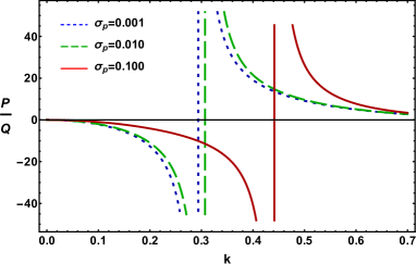
Figure 2: The variation of $P/Q$ with $k$ for different values of $\sigma_{p}$ when $\alpha=0.04$, $\gamma_{c}=0.5$, $\gamma_{h}=0.8$, $\sigma_{h}=0.01$, $q_{h}=1.3$, and $q_{p}=1.5$.

with the compatibility condition

$$V_{g}=\frac{\partial\omega}{\partial k}=\frac{\omega^{2}-S^{2}}{\omega k}.$$ (23)

The coefficients of $\epsilon$ for $m=2$ and $l=2$ provide the second order harmonic amplitudes which are found to be proportional to $|\phi_{1}^{(1)}|^{2}$

$$n_{i2}^{(2)}=A_{10}|\phi_{1}^{(1)}|^{2},$$ (24)

$$u_{i2}^{(2)}=A_{11}|\phi_{1}^{(1)}|^{2},$$ (25)

$$\phi_{2}^{(2)}=A_{12}|\phi_{1}^{(1)}|^{2},\$$ (26)

where

$$A_{10}=\frac{\alpha k^{6}+3\omega^{2}k^{4}+2A_{12}S^{2}k^{2}}{2S^{3}},~{}~{}A_{11}=\frac{\omega A_{10}S^{2}-\omega k^{4}}{kS^{2}},~{}~{}A_{12}=\frac{\alpha k^{6}+3\omega^{2}k^{4}-2A_{8}S^{3}}{2S^{3}(4k^{2}+A_{7})-2k^{2}S^{2}}.\$$

Now, we consider the expression for ($m=3$ with $l=0$) and ($m=2$ with $l=0$), which leads the zeroth harmonic modes. Thus, we obtain

$$n_{i0}^{(2)}=A_{13}|\phi_{1}^{(1)}|^{2},$$ (27)

$$u_{i0}^{(2)}=A_{14}|\phi_{1}^{(1)}|^{2},$$ (28)

$$\phi_{0}^{(2)}=A_{15}|\phi_{1}^{(1)}|^{2},\$$ (29)

where

$$A_{13}=\frac{2\omega V_{g}k^{3}+\alpha k^{4}+\omega^{2}k^{2}+A_{15}S^{2}}{S^{2}(V_{g}^{2}-\alpha)},~{}~{}~{}~{}A_{14}=\frac{A_{13}V_{g}S^{2}-2\omega k^{3}}{S^{2}},$$

$$A_{15}=\frac{2\omega V_{g}k^{3}+\alpha k^{4}+\omega^{2}k^{2}-2A_{8}S^{2}(V_{g}^{2}-\alpha)}{A_{7}S^{2}(V_{g}^{2}-\alpha)-S^{2}}.\$$

Finally, the third harmonic modes ($m=3$) and ($l=1$), with the help of Eqs. (18)-(29), give a set of equations, which can be reduced to the following NLSE:

$$i\frac{\partial\Phi}{\partial\tau}+P\frac{\partial^{2}\Phi}{\partial\xi^{2}}+Q|\Phi|^{2}\Phi=0,$$ (30)

where $\Phi=\phi_{1}^{(1)}$ for simplicity. In Eq. (30), $P$ is the dispersion coefficient which can be written as

$$P=\frac{V_{g}\alpha^{2}k^{5}-3V_{g}k\omega^{4}+4\alpha k^{2}\omega^{3}-4\omega\alpha^{2}k^{4}+2\alpha V_{g}\omega^{2}k^{3}}{2\omega^{2}k^{2}},\$$

and $Q$ is the nonlinear coefficient which can be written as

$$Q=\frac{2A_{8}S^{2}(A_{12}+A_{15})+3A_{9}S^{2}-(\omega^{2}k^{2}+\alpha k^{4})(A_{10}+A_{13})-2\omega k^{3}(A_{11}+A_{14})}{2\omega k^{2}},\$$

The space and time evolution of the IAWs in a FCPM are directly governed by the coefficients $P$ and $Q$, and indirectly governed by different plasma parameters such as $\alpha$, $\gamma_{c}$, $\gamma_{h}$, $\sigma_{h}$, $\sigma_{p}$, $q_{h}$, $q_{p}$, and $k$, etc. Thus, these plasma parameters can significantly modify the stability conditions of IAWs in a FCPM.

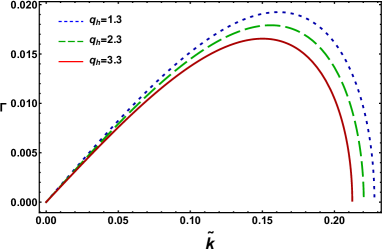
Figure 3: The variation of $\Gamma$ against $\widetilde{k}$ for different values of $q_{h}$ when $k=0.5$, $\phi_{0}=0.5$, $\alpha=0.04$, $\gamma_{c}=0.5$, $\gamma_{h}=0.8$, $\sigma_{h}=0.01$, $\sigma_{p}=0.01$, and $q_{p}=1.5$.

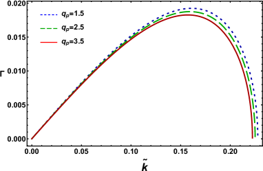
Figure 4: The variation of $\Gamma$ against $\widetilde{k}$ for different values of $q_{p}$ when $k=0.5$, $\phi_{0}=0.5$, $\alpha$=$0.04$, $\gamma_{c}=0.5$, $\gamma_{h}=0.8$, $\sigma_{h}$=$0.01$, $\sigma_{p}$=$0.01$, and $q_{h}=1.3$.

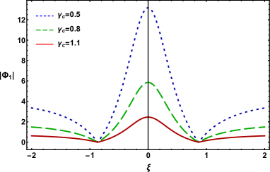
Figure 5: The variation of the $|\phi|$ with $\xi$ for different values of $\gamma_{c}$ when $k=0.5$, $\tau=0$, $\alpha=0.04$, $\gamma_{h}=0.8$, $\sigma_{h}=0.01$, $\sigma_{p}=0.01$, $q_{h}=1.3$, and $q_{p}=1.5$.

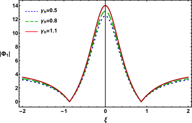
Figure 6: The variation of the $|\phi|$ with $\xi$ for different values of $\gamma_{h}$ when $k=0.5$, $\tau=0$, $\alpha=0.04$, $\gamma_{c}=0.5$, $\sigma_{h}=0.01$, $\sigma_{p}=0.01$, $q_{h}$=$1.3$, and $q_{p}=1.5$.

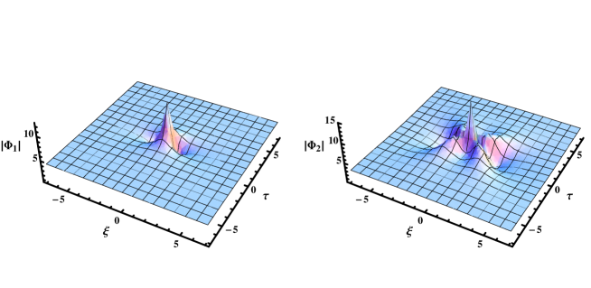
Figure 7: Profile of the first-order rational solution (left panel) and second-order rational solution (right panel) of NLSE at $k=0.5$.

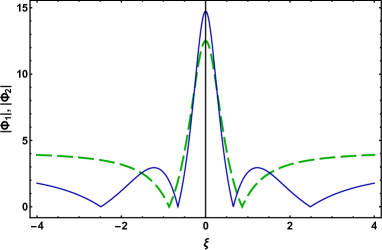
Figure 8: The variation of first-order (dashed green curve) and second-order (solid blue curve) rational solutions of NLSE at $k=0.5$ and $\tau=0$.

4 Modulational instability and Rogue waves

To study the MI of IAWs, we consider the linear solution of the Eq. (30) in the form $\Phi=\widetilde{\Phi}e^{iQ|\widetilde{\Phi}|^{2}\tau}$+c.c., where $\widetilde{\Phi}=\widetilde{\Phi}_{0}+\epsilon\widetilde{\Phi}_{1}$ and $\widetilde{\Phi}_{1}=\widetilde{\Phi}_{1,0}e^{i(\widetilde{k}\xi-\widetilde{\omega}{\tau})}+c.c$. We note that the amplitude depends on the frequency, and that the perturbed wave number $\widetilde{k}$ and frequency $\widetilde{\omega}$ which are different from $k$ and $\omega$. Now, substituting these into Eq. (30), one can easily obtain the following nonlinear dispersion relation [19, 20, 21]

$$\widetilde{\omega}^{2}=P^{2}\widetilde{k}^{2}\Big{(}\widetilde{k}^{2}-\frac{2|\widetilde{\Phi}_{0}|^{2}}{P/Q}\Big{)}.$$ (31)

It is observed here that the ratio $P/Q$ is negative (i.e., $P/Q<0$), the IAWs will be modulationally stable. On the other hand, if the ratio $P/Q$ is positive (i.e., $P/Q>0$), the IAWs will be modulationally unstable [19, 20, 21, 22, 23]. It is obvious from Eq. (31) that the IAWs becomes modulationally unstable when $\widetilde{k}_{c}>\widetilde{k}$ in the regime $P/Q>0$, where $\widetilde{k}_{c}=\sqrt{2(Q/P)}{|\widetilde{\Phi}_{0}|}$. The growth rate $\Gamma$ of the modulationally unstable IAWs is given by

$$\Gamma=|P|\widetilde{k}^{2}\sqrt{\frac{\widetilde{k}_{c}^{2}}{\widetilde{k}^{2}}-1}.$$ (32)

The NLSE (30) has a variety of rational solutions, among them there is a hierarchy of rational solution that are localized in both the $\xi$ and $\tau$ variables. The first-order rational solution of Eq. (30) can be written as [24, 25, 26, 27]

$$\Phi_{1}(\xi,\tau)=\sqrt{\frac{2P}{Q}}\Big{[}\frac{4+16i\tau P}{1+4\xi^{2}+16\tau^{2}P^{2}}-1\Big{]}\mbox{exp}(2i\tau P).$$ (33)

The interaction of the two or more first-order RWs can generate higher-order RWs which has a more complicated nonlinear structure. The second-order rational solution of Eq. (30) can be written as [24, 25, 26, 27]

$$\Phi_{2}(\xi,\tau)=\sqrt{\frac{P}{Q}}\Big{[}1+\frac{G_{2}(\xi,\tau)+iM_{2}(\xi,\tau)}{D_{2}(\xi,\tau)}\Big{]}\mbox{exp}(i\tau P),$$ (34)

where

$$G_{2}(\xi,\tau)=\frac{3}{8}-6(P\xi\tau)^{2}-10(P\tau)^{4}-\frac{3\xi^{2}}{2}-9(P\tau)^{2}-\frac{\xi^{4}}{2},$$

$$M_{2}(\xi,\tau)=-P\tau\Big{[}\xi^{4}+4(P\xi\tau)^{2}+4(P\tau)^{4}-3\xi^{2}+2(P\tau)^{2}-\frac{15}{4}\Big{]},$$

$$D_{2}(\xi,\tau)=\frac{\xi^{6}}{12}+\frac{\xi^{4}(P\tau)^{2}}{2}+\xi^{2}(P\tau)^{4}+\frac{2(P\tau)^{6}}{3}+\frac{\xi^{4}}{8}+\frac{9(P\tau)^{4}}{2}-\frac{3(P\xi\tau)^{2}}{2}+\frac{9\xi^{2}}{16}+\frac{33(P\tau)^{2}}{8}+\frac{3}{32}.\$$

The Eqs. (33) and (34) represent the profile of the first and second order IARWs associated with the IAWs in the modulationally unstable parametric regime (i.e., $P/Q>0$), respectively. We have numerically analyzed the first and second order IARWs in Figs. 5-8.

5 Results and discussion

Now, we would like to numerically analyze the stability conditions of the IAWs in presence of cold electrons following Maxwellian distribution, and hot electrons and positrons featuring $q$-distribution. The existence of two temperature electrons with distinct temperature and number density can be found in Saturn’s magnetosphere [4, 5, 6, 8, 7, 9], Auroral plasma [28, 29], Earth’s magnetosphere [30, 31], tandem mirror experiments [32], rf-heated plasma [33], and sputtering magnetron plasma [34], etc. The Saturn’s magnetosphere has three regions: the inner magnetosphere ($R\leq 9R_{s}$), intermediate magnetosphere ($9R_{s}<R<13R_{s}$), and outer magnetosphere ($\geq 13R_{s}$), where $R_{S}\approx 60,300$ km is the radius of Saturn. The components of the inner magnetosphere of Saturn are $N^{+}$, $O^{+}$, $OH^{+}$, $H_{2}O^{+}$, and neutral objects [36], etc. Schippers et al. [9] analysed the CAPS/ELS and MIMI/LEMMS data from the Cassini spacecraft orbiting Saturn over a range of $5.4-20R_{S}$ which can be found from Table 1.

Table 1: Parameter values derived from Schippers et al. [8, 9] corresponding to Saturn’s Magnetosphere

$R$ ($R_{s}$)	$T_{c}$ (eV)	$T_{h}$ (eV)	$n_{c}$ ($cm^{-3}$)	$n_{h}$ ($cm^{-3}$)
5.40	1.8	300	10.5	0.02
6.30	2.0	400	10.5	0.01
9.80	8.0	1100	2.50	0.07
12.0	6.0	1200	1.00	0.11
13.1	10.2	1000	0.21	0.18
14.0	30	900	0.15	0.10
15.2	70	900	0.25	0.10
17.8	28	1000	0.15	0.07

A number of authors numerically analyzed the effects of two distinct temperature (hot and cold) electrons following iso-thermal [1, 35] or non-thermal [2, 3, 4, 5, 6, 7, 8] distribution on the dynamics of space [1, 2, 3, 4, 5, 6, 7, 8] and laboratory [31, 33, 34, 35] plasma system under these assumptions: $T_{h}>T_{c}$ and $n_{h0}>n_{c0}$ [1, 3, 4, 5, 6, 7, 8, 31, 33, 35] or $n_{h0}=n_{c0}$ [5, 7, 8] or $n_{h0}<n_{c0}$ [2, 4, 6, 7, 8, 34, 35]. The parameters $q_{h},~{}q_{p}$ are the non-extensive parameter describing the degree of non-extensivity, i.e., $q_{h},~{}q_{p}=1$ corresponds to Maxwellian distribution, whereas $q_{h},~{}q_{p}<1$ refers to the super-extensivity, and the opposite condition $q_{h},~{}q_{p}>1$ refers to the sub-extensivity. This means that in the dynamics of electrons and positrons, all the forces (including the force leading to annihilation of electrons and positrons [37, 38]) except the forces arising from electrostatic wave potential, thermal pressure of electrons and positrons, and deviation from Maxwellian to non-extensive $q$-distribution have been neglected. Therefore, in our present investigation, we have considered for our numerical analysis that $T_{h}=T_{p}=(10-1000)T_{c}$, $T_{i}=0.1T_{c}$ [7, 33], $Z=1-20$ [2, 3, 4, 5, 6, 7, 8], $n_{h0}>n_{c0}$, $n_{h0}=n_{c0}$, $n_{h0}<n_{c0}$, and small fraction of positrons.

The variation of $P/Q$ with $k$ for different values of $\sigma_{h}$ and $\sigma_{p}$ can be seen in Figs. 1 and 2, respectively, and these figures can highlight the effects of temperature of the hot electron and positron as well as cold electron species on the modulationally stable and unstable parametric regimes of IAWs in FCPM. It is clear from these figures that (i) both stable and unstable parametric regimes are allowed by the FCPM; (ii) the $k_{c}$ increases with the increase in the value of both $\sigma_{h}$ and $\sigma_{p}$; (iii) the physics of this result is that the nonlinearity of the plasma medium increases with the increase of both hot electron and positron temperature for constant temperature of the cold electrons, and this would lead the IAWs become unstable for small values of $k$ as well as allows to generate the first and second order IARWs in the modulationally unstable parametric regime (i.e., $k>k_{c}$).

We have numerically analyzed Eq. (32) in Figs. 3 and 4 to observed that how the nonlinearity as well as the growth rate of the IAWs changes with $\widetilde{k}$ for different values of the non-extensivity of hot electrons (via $q_{h}$) and hot positrons (via $q_{p}$), and it is obvious from these figures that an increase in the value of the $q_{h}$ (in Fig. 3) or $q_{p}$ (in Fig. 4) does not only cause to decrease the nonlinearity of the FCPM but also causes to decrease the maximum value of the growth rate. The physics of the result is that the distribution function with $q<1$, compared with the Maxwellian one ($q=1$) indicates the system with more super-thermal particles (super-extensivity) whereas the $q$-distribution with $q>1$ is suitable for plasma containing a large number low-speed particles (sub-extensivity). This means that our FCPM has large number low-speed particles which reduce the nonlinearity as well as the maximum value of the growth rate with $q_{h}$ and $q_{p}$.

Figure 5 and 6 indicate how the nonlinearity of FCPM as well as the configuration of the IARWs associated with IAWs in the modulationally unstable parametric regime (i.e., $P/Q>0$) changes with the charge state of positive ion and also the number density of cold and hot electrons, and warm ions. The amplitude and the width of the IARWs decrease with an increase in the value of the cold electron number density for a constant value of the charge state and number density of the warm ions (via $\gamma_{c}$ and can be seen from Fig. 5). On the other hand, the existence of large amount of hot electrons increases the amplitude and width of the IARWs associated with IAWS when other plasma parameters remain constant (via $\gamma_{h}$ and can be seen from Fig. 6). These two interesting phenomena may be explained in physical framework as follows: an increase in cold (hot) electron number density could shrink (enhance) the nonlinearity of the FCPM and disperse (concentrate) its energy which makes the amplitude and width of the IARWs shorter and narrower (taller and wider).

The time evolution and the comparison of the first and second order IARW associated with IAW in the modulationally unstable parametric regime can be seen from Figs. 7 and 8, respectively. Figure 8 indicates the comparison of the first and second order IARW solutions at $\tau=0$, and it is clear from this figure that (a) the second-order IARW has double structures compared with the first-order IARW; (b) the amplitude of the second-order IARW is always greater than the amplitude of the first-order IARW; (c) the potential profile of the second-order IARW becomes more spiky (i.e., the taller amplitude and narrower width) than the first-order IARW; (d) the second (first) order IARW has four (two) zeros symmetrically located on the $\xi$-axis; (e) the second (first) order IARW has three (one) local maxima.

6 Conclusion

We have considered a more general and realistic four component plasma model, and have investigated the stable and unstable parametric regimes, which can be recognized by the sign of the coefficients $P$ and $Q$ of NLSE, of IAWs. The $k_{c}$ value, which divides the stable and unstable parametric regimes of IAWs, totally depends on the temperature of hot and cold electrons. An increase in the value of the $q_{h}$ or $q_{p}$ does not only cause to decrease the nonlinearity of the FCPM but also causes to decrease the maximum value of the growth rate. The numerical analysis has also shown that the amplitude and width of the IARWs increase with an increase in the value of hot electron number density while decrease with an increase in the value of cold electron number when other plasma parameters remain constant. Finally, the finding of our present investigation may be applicable in explaining the formation of the IARWs in Saturn’s magnetosphere [4, 5, 6, 8, 7, 9], Auroral plasma [28, 29], Earth’s magnetosphere [30, 31], tandem mirror experiments [32], rf-heated plasma [33], and sputtering magnetron plasma [34], etc.

References

- [1] M.A. Rehman, M.K. Mishra, Phys. Plasmas 23 (2016) 012302.
- [2] M. Shahmansouri, H. Alinejad, Phys. plasmas 24 (2017) 113701.
- [3] Shalini, N.S. Saini, A.P. Misra, Phys. Plasmas 22 (2015) 092124.
- [4] A. Panwar, C.M. Ryu, A.S. Bains, Phys. Plasmas 21 (2014) 122105.
- [5] I. Kourakis, P.K. Shukla, J. Phys. A Math. Gen. 36 (2003) 11901.
- [6] H. Alinejad, M. Mahdavi, M. Shahmansouri, Astrophys. Space Sci. 352 (2014) 571.
- [7] T.K. Baluku, M.A. Hellberg, Vacuum 147 (2018) 31.
- [8] T.K. Baluku, M.A. Hellberg, R.L. Mace, J. Geophys. Res. 116 (2011) A04227.
- [9] P. Schippers, M. Blanc, et al., J. Geophys. Res. 113 (2008) A07208.
- [10] E.C. Sittler, K.W. Ogilvie, J.D. Scudder, J. Geophys. Res. 88 (1983) 8847.
- [11] D.D. Barbosa, W.S. Kurth, J. Geophys. Res. 98 (1993) 9351.
- [12] D.T. Young, J.J. Berthelier, et al., Science 307 (2005) 1262.
- [13] N. Ahmed, A. Mannan, N.A. Chowdhury, A.A. Mamun, Chaos 28 (2018) 123107.
- [14] S. Khondaker, N.A. Chowdhury, A. Mannan, A.A. Mamun, arXiv:1809.09312.
- [15] N. A. Chowdhury, A. Mannan, M.M. Hasan, A.A. Mamun, Chaos 27 (2017) 093105.
- [16] M.H. Rahman, N.A. Chowdhury, A. Mannan, et al., Chinese J. Phys. 56 (2018) 2061.
- [17] S. Jahan, N.A. Chowdhury, A. Mannan, A.A. Mamun, Commun. Theor. Phys. 71 (2019) 327.
- [18] M.H. Rahman, A. Mannan, N.A. Chowdhury, A.A. Mamun, Phys. Plasmas 25 (2018) 102118.
- [19] N.A. Chowdhury, A. Mannan, M.M. Hasan, and A.A. Mamun, Plasma Phys. Rep. 45 (2019) 459.
- [20] I. Kourakis, P.K. Sukla, Nonlinear Proc. Geophys. 12 (2005) 407.
- [21] S. Sultana, I. Kourakis, Plasma Phys. Control. Fusion 53 (2011) 045003.
- [22] R. Fedele, H. Schamel, Eur. Phys. J. D 73 (2019) 177.
- [23] R. Fedele, Phys. Scr. 65 (2002) 502.
- [24] A. Ankiewicz, P.A. Clarkson, N. Akhmediev, J. Phys. A 43 (2010) 12002.
- [25] S. Guo, L. Mei, W. Shi, Contrib. Plasma Phys. 58 (2018) 870.
- [26] S. Guo, L. Mei, Phys. Plasmas 21 (2014) 112303.
- [27] Z. Yan, Commun. Theor. Phys. 71 (2019) 1017.
- [28] M. Temerin, K. Cerny, W. Lotko, F.S. Mozer, Phys. Rev. Lett. 48 (1982) 1175.
- [29] R. Bostrom, G. Gustafsson, et al., Phys. Rev. Lett. 61 (1988) 82.
- [30] J.D. Gaffey, R.E. LaQuey, J. Geophys. Res. 81 (1976) 595.
- [31] S.S. Ghosha, A.N.S. Iyengar, Phys. Plasmas 4 (1997) 3204.
- [32] J. Kesner, Nucl. Fusion 25 (1985) 275.
- [33] Y. Nishida, T. Nagasawa, Phys. Fluids 29 (1986) 345.
- [34] T. E. Sheridan, M.J. Goeckner, J. Goree, J. Vacuum Sci. Tech. A 9 (1991) 688.
- [35] S. Baboolal, R. Bharuthram, M.A. Hellberg, J. Plasma Phys. 41 (1989) 341.
- [36] N. Krupp, A. Lagg, J. Woch, et al., Geophys. Res. Lett. 32 (2005) L20S03.
- [37] I. Kourakis, A. Esfandyari-Khalejahi, et al., Phys. Plasmas 13 (2006) 052117.
- [38] A. Esfandyari-Khalejahi, I. Kourakis, et al., J. Phys. A 39 (2006) 13817.