Managing Variability in Relational Databases by VDBMS

Abstract.

Variability inherently exists in databases in various contexts which creates database variants. For example, variants of a database could have different schemas/content (database evolution problem), variants of a database could root from different sources (data integration problem), variants of a database could be deployed differently for specific application domain (deploying a database for different configurations of a software system), etc. Unfortunately, while there are specific solutions to each of the problems arising in these contexts, there is no general solution that accounts for variability in databases and addresses managing variability within a database. In this paper, we formally define variational databases (VDBs) and statically-typed variational relational algebra (VRA) to query VDBs—both database and queries explicitly account for variation. We also design and implement variational database management system (VDBMS) to run variational queries over a VDB effectively and efficiently. To assess this, we generate two VDBs from real-world databases in the context of software development and database evolution with a set of experimental queries for each.

1. Introduction

Data and variants of data are abundant. Having variants of data is unavoidable, it needs to be maintained, and it appears in multiple context. While there are solutions dealing with variants of data in specific contexts, there is no general solution to the problem of accounting for variability in data. In this section, we focus on variability in relational databases in different contexts that already exists in the field, current solutions that address them, and their shortcomings.

Context 1: schema evolution. One way that data variants arise is when a database schema evolves over time— an unpredictable and inevitable occurrence which is independent from how good or bad the initial schema has been designed (Stonebraker et al., 2016). Although, there are guidelines that direct database administrators (DBAs) to design schemas that do not rapidly decay over time, in practice, there is still no way to avoid the change due to business circumstances, mergers and acquisitions, and new applications for the same data (Stonebraker et al., 2016). Every time the database evolves, a new “variant” is created.

Current solutions addressing schema evolution require DBAs to design a unified schema, map old schema to the unified one, and migrate the database to keep the old variants of database (Moon et al., 2008). They also require DBAs (and/or application developers) to rewrite queries which were based on the previous schema. These approaches have multiple limitations: 1) they are time-consuming, error-prone, and burdensome tasks for DBAs and developers and 2) users cannot access any of the old variants even if they desire. Some of the recent solutions address these issues to some extent, but induce other limitations on the problem, explored more in § 2.

Context 2: data integration. Another kind of common variation in data arises from the integration of multiple different data sources into a single database, i.e., data integration (Doan et al., 2012). Each data source is a data variant. Assuming that all sources have the same format (e.g., they are all relational databases), they still could differ in details such as their schema.

Existing solutions for integrating all variants requires the capability to adjust all databases to a unified database. For example, in the case of relational databases, we need to map all schemas to a unified schema (Doan et al., 2012). Here, the variants of data come from different sources that need to be combined systematically. The problem with unifying all the variants into a unified database is that queries cannot specify a unique source to inquire information from, the same problem appeares in schema evolution. Furthermore, in this context, a user’s inquiry result is collected from all variants and presented to the user. Unfortunately, there is no way for the user to identify which variant a specific piece of result (e.g., a tuple in the case of relational databases) belongs to, i.e., data integration systems lose data provenance (Doan et al., 2012).

Context 3: Software Product Lines. Additionally, data variants arises as the artifact of software development, evolution, and maintenance, especially in the context of software product line (SPL). SPL is an approach to developing and maintaining software-intensive systems in a cost-effective, easy to maintain manner. The products of a SPL pertain to a common application domain or business goal. They also have a common managed set of features that describe the specific need for a product. They share a common codebase which is used to produce a product with respect to its set of selected (enabled) features (, 2001). Different products of a SPL typically have different sets of features or are tailored to run in different environments. These differences impose different data requirements. For example, different legal requirements often require tracking different data in products tailored for use in different countries or regions.

In practice, software systems produced by a SPL are accommodated with a database that has all attributes and tables available in all variants– a global database (Ataei et al., 2018). Unfortunately, this approach is inefficient, error-prone, and filled with lots of null values since not all attributes and tables are valid for all variant products.

As shown thus far, variability in databases is abundant, inevitable, inexorable, and impacts DBAs, data scientists, and developers significantly. Various research addresses instances of introduction/existence of variability into/in a database such as schema evolution, although these customized solutions have some shortcomings within and beyond their own context. Current approaches are limited because they dismiss that: the problem at hand is essentially an instance of introduction/existence of variability into/in a database.

To solve this problem, we need to resolve the challenge of how to incorporate variability in databases to allow for expressive and efficient queries that satisfy the general needs of different contexts where variability appears? Our contributions in this paper address this challenge:

• We provide a framework to capture variability within a database using propositional formulas over sets of features, called feature expressions, following (Ataei et al., 2017).

• We incorporate feature expressions into both the content (tuples) and structure (schema) of the database, introducing variational schemas, § 4.1, and variational tables, § 4.2, and together VDBs, § 4.

• To express user information needs we define a domain-specific language which is a combination of relational algebra and choice calculus (Erwig and Walkingshaw, 2011; Walkingshaw, 2013), § 5.1, that allows users to query a VDB by a variational query (v-query), § 5.

• We define a static type system for our language, § 5.2, along with rules to minimize variation within a v-query, § 5.3.

• To efficiently query a variational database and receive effective clear results we introduce Variational Database Management System (VDBMS), § 6.

To evaluate VDBMS, we adopt two real-world databases (employee database and Enron email data corpus) from two different contexts (schema evolution and SPL), generate their counterpart VDBs (based on the changes applied to them), assess the performance of VDBMS using a set of reasonable queries within each context, and finally analyze and discuss the results, § 7.

2. Motivating Example

Table 1. Schema evolution of an employee database for a SPL. A feature (a boolean variable) represents an optional inclusion of a schema or elements of a schema. The dash-underlined attributes in left schema column only exist when the education feature of SPL is enabled. This table represents 1056 possible schema variants ($2^{5}$ schema variants when $\mathit{edu}$ is disabled in addition to $2^{5}\times 2^{5}$ when $\mathit{edu}$ is enabled).

Temporal	SPL Features		Temporal
Features	$\mathit{edu}\vee\neg\mathit{edu}\equiv\textrm{\small{true}}$	$\mathit{edu}$	Features
$V_{1}$	$\mathit{engineerpersonnel}$ ($\mathit{empno}$, $\mathit{name}$, $\mathit{hiredate}$,$\mathit{title}$,$\mathit{deptname}$)	$\mathit{course}$ ($\mathit{coursename}$, $\mathit{teacherno}$)	$T_{1}$
	$\mathit{otherpersonnel}$ ($\mathit{empno}$, $\mathit{name}$, $\mathit{hiredate}$, , $\mathit{deptname}$)	$\mathit{student}$ ($\mathit{studentno}$, $\mathit{coursename}$)
	$\mathit{job}$ ($\mathit{title}$, $\mathit{salary}$)
$V_{2}$	$\mathit{empacct}$ ($\mathit{empno}$, $\mathit{name}$, $\mathit{hiredate}$, $\mathit{title}$, $\mathit{deptname}$)	$\mathit{course}$ ($\mathit{courseno}$, $\mathit{coursename}$, $\mathit{teacherno}$)	$T_{2}$
	$\mathit{job}$ ($\mathit{title}$, $\mathit{salary}$)	$\mathit{student}$ ($\mathit{studentno}$, $\mathit{courseno}$)
$V_{3}$	$\mathit{empacct}$ ($\mathit{empno}$, $\mathit{name}$, $\mathit{hiredate}$, $\mathit{title}$, $\mathit{deptno}$)	$\mathit{course}$ ($\mathit{courseno}$, $\mathit{coursename}$)	$T_{3}$
	$\mathit{job}$ ($\mathit{title}$, $\mathit{salary}$)	$\mathit{teach}$ ($\mathit{teacherno}$, $\mathit{courseno}$)
	$\mathit{dept}$ ($\mathit{deptname}$, $\mathit{deptno}$, $\mathit{managerno}$)	$\mathit{student}$ ($\mathit{studentno}$, $\mathit{courseno}$, $\mathit{grade}$)
	$\mathit{empbio}$ ($\mathit{empno}$, $\mathit{sex}$, $\mathit{birthdate}$)
$V_{4}$	$\mathit{empacct}$ ($\mathit{empno}$, $\mathit{hiredate}$, $\mathit{title}$, $\mathit{deptno}$, $\mathit{std}$, $\mathit{instr}$)	$\mathit{ecourse}$ ($\mathit{courseno}$, $\mathit{coursename}$)	$T_{4}$
	$\mathit{job}$ ($\mathit{title}$, $\mathit{salary}$)	$\mathit{course}$ ($\mathit{courseno}$, $\mathit{coursename}$, $\mathit{time}$, $\mathit{class}$)
	$\mathit{dept}$ ($\mathit{deptname}$, $\mathit{deptno}$, $\mathit{managerno}$)	$\mathit{teach}$ ($\mathit{teacherno}$, $\mathit{courseno}$)
	$\mathit{empbio}$ ($\mathit{empno}$, $\mathit{sex}$, $\mathit{birthdate}$, $\mathit{name}$)	$\mathit{student}$ ($\mathit{studentno}$, $\mathit{courseno}$, $\mathit{grade}$)
$V_{5}$	$\mathit{empacct}$ ($\mathit{empno}$, $\mathit{hiredate}$, $\mathit{title}$, $\mathit{deptno}$, $\mathit{std}$, $\mathit{instr}$, $\mathit{salary}$)	$\mathit{ecourse}$ ($\mathit{courseno}$, $\mathit{coursename}$, $\mathit{deptno}$)	$T_{5}$
	$\mathit{dept}$ ($\mathit{deptname}$, $\mathit{deptno}$, $\mathit{managerno}$, $\mathit{stdnum}$, $\mathit{instrnum}$)	$\mathit{course}$ ($\mathit{courseno}$, $\mathit{coursename}$, $\mathit{time}$, $\mathit{class}$, $\mathit{deptno}$)
	$\mathit{empbio}$ ($\mathit{empno}$, $\mathit{sex}$, $\mathit{birthdate}$, $\mathit{firstname}$, $\mathit{lastname}$)	$\mathit{teach}$ ($\mathit{teacherno}$, $\mathit{courseno}$)
		$\mathit{take}$ ($\mathit{studentno}$, $\mathit{courseno}$, $\mathit{grade}$)

Encoding variability into databases is more critical when multiple contexts meet. An existing example of this is when the evolution of a SPL results in its database schema evolution (Herrmann et al., 2015). Database evolution within a SPL happens at two stages: 1) component evolution: developers update, refactor, improve, and components resulting in potentially changing the data model, i.e., the database schema, and 2) product evolution: clients want to add/remove a feature or component which potentially propagates to database evolution (Herrmann et al., 2015; Botterweck and Pleuss, 2014).

Products of a SPL require different variants of a database to store their information, if any, since each product desires to store some specific information that others may not care about. These database variants differ mainly in their schema, a relation/attribute can either be included or excluded for a specific software product and the feature set for a product determines which relations and attributes to include in its database, i.e., the features dictate the database schema (Ataei et al., 2018). In practice, SPLs use a unified schema for all database variants—an error-prone approach resulting in lots of null values for attributes that do not exists in a database variant.

We illustrate an example of database schema evolution within a SPL in an employee database. We use parts of this example as our running example throughout the paper. Table 1 outlines schema variations of our example. The schema consists of two sub-schemas, the left one (the second column from left) stores employees information and the right one stores education-related information of employees while they are working at the company. It has three dimensions of variability. The horizontal axis accounts for SPL features—for brevity, we consider an SPL that has only one feature: $\mathit{edu}$, if the $\mathit{edu}$ feature is enabled the database schema includes the education sub-schema in addition to the employee sub-schema, otherwise it only consists of the employee sub-schema. The vertical axes on the left and right account for the other two dimensions, representing temporal changes to the employee and education sub-schemas, respectively. The sub-schemas evolve over time due to business requirements (Moon et al., 2008), potentially with different paces which requires two different dimensions of variability to capture each of them individually. We use temporal features to refer to each time a schema evolves. Enabling a temporal feature indicates that its corresponding database variants include the sub-schema associated with the feature. E.g., if $V_{1}$ is enabled the schema includes $\mathit{engineerpersonnel}$, $\mathit{otherpersonnel}$, and $\mathit{job}$.

We describe the schema variations shown in Table 1 w.r.t. SPL component evolution (when developers introduce new changes). The database initially has three tables for all SPL products: $\mathit{engineerpersonnel}$, $\mathit{otherpersonnel}$, and $\mathit{job}$. In addition to these it has two tables $\mathit{course}$ and $\mathit{student}$ for SPL products providing education. Note that teachers and students are both assumed to be employees.

To uniformly manage employee information, in variants of $V_{2}$, SPL developers decide to combine $\mathit{engineerpersonnel}$ and $\mathit{otherpersonnel}$ into one table $\mathit{empacct}$. At the same time, in variants of $T_{2}$, due to increase in number of courses offered the $\mathit{courseno}$ attribute is added to $\mathit{course}$ table.

As companies grow, in temporal variants of $V_{3}$, the $\mathit{dept}$ and $\mathit{empbio}$ tables are added. Similarly for variants of $T_{3}$, the $\mathit{teach}$ table is added in addition to the $\mathit{grade}$ attribute in the $\mathit{student}$ table to account for employees attempt to better themselves.

Within $V_{4}$ schema variants, the $\mathit{name}$ attribute is moved from the $\mathit{empacct}$ table to the $\mathit{empbio}$ table. Also, due to an increase of the number of employees who take courses, attributes $\mathit{std}$ and $\mathit{instr}$ are added to $\mathit{empacct}$ to account for an employee being a student and/or teacher, respectively. Note that these attributes only exists in a schema if the company offers education to its employees. In temporal variants of $T_{4}$, due to the high requests of employees, e-courses are offered, hence, the $\mathit{ecourse}$ table is added. Note that we could have a different design and consider offering e-courses as a SPL feature.

Eventually, to motivate employees the companies of temporal variants $V_{5}$ consider salary dependent on the employee and not the title. Hence, the $\mathit{salary}$ attribute is added to the $\mathit{empacct}$ table and the $\mathit{job}$ table is dropped. To access statistics of departments for educational purpose, attributes $\mathit{stdnum}$ and $\mathit{instrnum}$ are added to $\mathit{dept}$ relation when $\mathit{edu}$ is enabled. Additionally, the first name and last name of employees is stored separately and the $\mathit{student}$ table is renamed to $\mathit{take}$.

The schema also evolves due to product evolution, i.e., a client requests a new version. For example, consider a client that previously has requested software with database variant associated with $V_{5}$. Now the client decides to educate its employees. Hence, the SPL developers need to reconfigure the product for such a client to meet their needs. The schema evolution described above also captures product evolution.

As mentioned earlier, existing solutions burden DBAs heavily by requiring them to define a unified schema, map old schemas to the unified one, migrate the data, and rewrite queries (Curino et al., 2008). Some approaches automate schema mapping when the schema evolves to migrate the data, however, they still require the DBA to rewrite queries (Velegrakis et al., 2003; Yu and Popa, 2005). Other solutions, keep some sort of history of database evolution and either allow the user to specify the version of the database their query is written again and generate queries for all other versions (Moon et al., 2008). The specific problem of schema evolution when a SPL evolves is addressed by designing a new domain-specific language so that SPL developers can write scripts of the schema changes (Herrmann et al., 2015), which still requires a great effort by DBAs and SPL developers. This amount of work grows exponentially as the number of potential variants grow, which in our example depends on the temporal changes and SPL features. As a reminder, a SPL usually has hundreds of features (Liebig et al., 2010). As the SPL and its database evolve, manually managing the variants becomes impossible.

Although current approaches address variability in specific applications and they provide interesting efficient solutions, they are tailored to the underlying application and thus fail to address the more general problem. This results in a pressing need of incorporating variability within databases in a flexible manner that can be applied in various context which we address by introducing variational databases and VDBMS to interact with them.

3. Preliminaries

In this section, we introduce concepts and notations that we use throughout the paper. Table 2 provides a short overview and is meant as an aid to find definitions faster. Throughout the paper, we discuss relational concepts and their variational counterparts. For clarity, when we need to emphasize an entity is not variational we underline it, e.g., $\underline{x}$ is a non-variational entity while $x$ is its potentially counterpart.

Table 2. Introduced notations and terminologies with their corresponding section(s).

Name	Notation	§
Feature	$f$	§ 3.2
Feature expression	$e$
Annotated element $x$ by $e$	${x}^{e}$
Configuration	$c$
True feature set of $c$	$e_{c}^{t}$
Evaluation of $e$ under $c$	$\mathbb{E}\llbracket e\rrbracket_{c}$
Presence condition of entity $x$	$pc\left(x\right)$
Optional attribute	$a$	§ 4.1
Variational attribute set	$A$
Variational relation schema	$s$
Variational schema	$S$
Variational tuple	$u$	§ 4.2
Variational relation content	$U$
Variational table	$t$= ($s$, $U$)
Choice	$e\langle x,y\rangle$	§ 5.1
Variational condition	$\theta$
Variational query	$q$
Configure query $q$ with configuration $c$	$\mathbb{Q}\llbracket q\rrbracket_{c}$	§ 5.1.1
Group query $q$	$\mathcal{Q}\left({q}\right)$

3.1. Relational Databases

A relational database $\underline{D}$ stores information in a structured manner by forcing data to conform to a schema $\underline{S}$ that is a finite set $\{{\underline{s}}_{1},\ldots,{\underline{s}}_{n}\}$ of relation schemas. A relation schema is defined as $\underline{s}=\underline{r}\left(\underline{a}_{1},\ldots,\underline{a}_{k}\right)$ where each $\underline{a}_{i}$ is an attribute of the relation $\underline{r}$. The function $rel\left(\underline{a}\right)$ returns the relation of an attribute. The function $\mathit{type}\left(\underline{a}\right)$ returns the type of attribute $\underline{a}$.

The content of database $\underline{D}$ is stored in the form of tuples. A tuple $\underline{u}$ is a mapping between a list of relation schema attributes and their values, i.e., $\underline{u}=\left(\underline{v}_{1},\ldots,\underline{v}_{k}\right)$ for the relation schema $\underline{r}$$\left(\underline{a}_{1},\ldots,\underline{a}_{k}\right)$. Hence a relation content, $\underline{U}$, is a set of tuples $\{\underline{u}_{1},\ldots,\underline{u}_{m}\}$. The function $att\left(\underline{v}\right)$ returns the attribute of a value. A table $\underline{t}$is a pair of relation content and relation schema. A database instance, $\underline{\mathcal{I}}$, of the database $\underline{D}$ with the schema $\underline{S}$, is a set of relation contents $\{{\underline{U}}_{1},\ldots,{\underline{U}}_{n}\}$ corresponding to a set of relation schemas $\{{\underline{s}}_{1},\ldots,{\underline{s}}_{n}\}$ defined in $\underline{S}$. For brevity, when it is clear from the context we refer to a database instance by database.

3.2. Encoding Variability

The first challenge of incorporating variability into a database is to represent variability. To represent variability we require a set of features, denoted by $\mathbf{F}$, appropriate for the context that the database is used for. For example, for the context of schema evolution, features can be generated from version numbers (e.g., features $V_{1}$ to $V_{5}$ and $T_{1}$ to $T_{5}$ in the motivating example, Table 1); for SPLs, the features can be adopted from the SPL feature set (e.g.: the $\mathit{edu}$ feature in our motivating example, Table 1); and for data integration, the features can demonstrate resources. For simplicity and without loss of generality, features are assumed to be boolean variables, although, it is easy to extend them to multi-valued variables.

Assuming that all the features by default are set to false, enabling some of them specifies a variant. Hence, to specify a variant we define a function, called a configuration, that maps every feature in the feature set to a boolean value. By definition, a configuration is a total function, i.e., it includes all features defined in the feature set. For brevity, we represent a configuration $c$ with a set of enabled features which represents a variant. E.g., the configuration $\{V_{2},T_{3},\mathit{edu}\}$ represents a database variant with employee sub-schema associated with $V_{2}$ and education sub-schema associated with $T_{3}$in Table 1.

Having defined a set of features, we also need to incorporate them into the database. To represent features in the database, we construct propositional formulas of features (which are basically boolean variables), describing the condition (circumstance) where one or more variant are valid, i.e., assigning features to their values defined in variant’s configuration and evaluating the propositional formula results in true. For example, the propositional formula $\neg\mathit{edu}$ represents all variants of our motivating example that do not have the education part of the schema, i.e., variant schemas of the left schema column.

We call propositional formula of features feature expression and define it formally in Figure 1. We define the syntax of feature expressions in Figure 1. Feature expression semantics, denoted by $\mathbb{E}\llbracket e\rrbracket_{c}:\mathbf{E}\to\mathbf{C}\to\mathbf{B}$, evaluates feature expression $e$ under configuration $c$, also called configuration of feature expression $e$ under $c$. For example, $\mathbb{E}\llbracket A\vee B\rrbracket_{\{A\}}=\textrm{\small{true}}$ Figure 1 defines the syntax and equivalence of two feature expressions. However, we define the evaluation of feature expressions and functions over them in Appendix A. We define two functions over feature expressions, as shown in Figure 1: 1) satisfiability: feature expression $e$ is satisfiable if there exists configuration $c$ s.t. $\mathbb{E}\llbracket e\rrbracket_{c}$= true and 2) tautology: feature expression $e$ is a tautology if for all valid configurations we have: $\mathbb{E}\llbracket e\rrbracket_{c}$= true.

To incorporate feature expressions into the database, we annotate/tag database elements (including attributes, relations, and tuples) with feature expressions. An annotated element $x$ with feature expression $e$ is denoted by ${x}^{e}$ where conceptually, feature expression $e$ represents a group of configuration where their variants contain element $x$. The feature expression attached to an element is called a presence condition since it determines the condition under which the element is valid. The function $pc\left(x\right)$ returns the presence condition of the element $x$. For example, the annotated number $2^{A}$ indicates that the number 2 is valid only when feature $A$ is enabled. Here, $pc\left(2\right)=A$.

No matter the context, features often times have a relationship with each other that constrains configurations. For example, only one of the temporal features of $V_{1}$– $V_{5}$ can be true for a given variant. This relationship can easily be captured by a feature expression, called a feature model, which restricts the set of valid configurations, i.e., if configuration $c$ violates the relationship then evaluating the feature model $m$ under this configuration evaluates to false: $\mathbb{E}\llbracket m\rrbracket_{c}$= false. For example, the restriction that at a given time only one employee schema is valid is represented by the feature expression: $\left(V_{1}\wedge\neg\left(V_{2}\vee\ldots\vee V_{5}\right)\right)\vee\left(V_{2}\wedge\neg\left(V_{1}\vee V_{3}\vee V_{4}\vee V_{5}\right)\right)\vee\ldots\vee\left(V_{5}\wedge\neg\left(V_{1}\vee\ldots\vee V_{4}\right)\right)$. Note that this is not the feature model for the entire motivating example.

Feature expression generic object:

$$\begin{array}[]{rcl@{\quad}l}f\in\mathbf{F}&\textit{Feature Name}\end{array}$$

Feature expression syntax:

$$\begin{array}[]{rcl@{\quad}l}b\in\mathbf{B}&\Coloneqq&\textrm{\small{true}}\hskip 6.45831pt|\hskip 6.45831pt\textrm{\small{false}}&\textit{Boolean Value}\\ e\in\mathbf{E}&\Coloneqq&b\hskip 6.45831pt|\hskip 6.45831ptf\hskip 6.45831pt|\hskip 6.45831pt\neg f\hskip 6.45831pt|\hskip 6.45831pte\wedge e\hskip 6.45831pt|\hskip 6.45831pte\vee e&\textit{Feature Expression}\\ c\in\mathbf{C}&=&\mathbf{F}\to\mathbf{B}&\textit{Configuration}\end{array}$$

Feature expression equivalence:

$$\mbox{$e$}_{1}\equiv e_{2}\textit{ iff \ }\forall c\in\mathbf{C}:\mathbb{E}\llbracket e_{1}\rrbracket_{c}=\mathbb{E}\llbracket e_{2}\rrbracket_{c}$$

Figure 1. Feature expression syntax and equivalence.

3.3. Variational Set

A variational set (v-set) $X=\{{x_{1}}^{e_{1}},\ldots,{x_{n}}^{e_{n}}\}$ is a set of annotated elements where the presence condition of elements is satisfiable (Erwig et al., 2013; Walkingshaw et al., 2014; Ataei et al., 2017). Conceptually, a variational set represents many different plain sets that can be generated by enabling or disabling features and including only the elements whose feature expressions evaluate to true, i.e., a variational set is a function from a configuration of its features to the corresponding plain set. A plain set is denoted by $\underline{X}$ while a variational set of non-variational elements is denoted by $\ddot{}\underline{X}$. We typically omit the feature expression true in a variational set, e.g., the v-set $\{{2}^{f_{1}},{3}^{f_{2}},4\}$ represents four plain sets under different configurations: $\{2,3,4\}$ when $f_{1}$ and $f_{2}$ are enabled, $\{2,4\}$ when $f_{1}$ is enable but $f_{2}$ is disabled, $\{3,4\}$ when $f_{2}$ is enabled but $f_{1}$ is disabled, and $\{4\}$ when both $f_{1}$ and $f_{2}$ are disabled.

A variational set itself can also be annotated with a feature expression. An annotated variational set ${X}^{e}=\{{x_{1}}^{e_{1}},\ldots,{x_{n}}^{e_{n}}\}^{e}$ is a v-set that it is annotated itself by a feature expression $e$. In essence, annotating a v-set with the feature expression $e$ restricts the condition under which its elements are valid, i.e., it forces elements’ presence conditions to be more specific. This restriction can be captured by the property: $\{{x_{1}}^{e_{1}},\ldots,{x_{n}}^{e_{n}}\}^{e}\equiv\{{x_{1}}^{e_{1}\wedge e},\ldots,{x_{n}}^{e_{n}\wedge e}\}$. For example, the annotated variational set $\{{2}^{f_{1}},{3}^{\neg f_{2}},4,{5}^{f_{3}}\}^{f_{1}\wedge f_{2}}$ indicates that all the elements of the set can only exists when both $f_{1}$ and $f_{2}$ are enabled. Thus, it is equivalent to $\{{2}^{f_{1}\wedge f_{2}},{4}^{f_{1}\wedge f_{2}},{5}^{f_{1}\wedge f_{2}\wedge f_{3}}\}$. The element $3$ is dropped from the set since its presence condition is unsatisfiable, i.e., $\neg\mathit{sat}\left(\neg f_{2}\wedge(f_{1}\wedge f_{2})\right)$.

We provide operation definitions over v-sets. These operations are vastly used in § 5.2.

Definition 3.1 (V-set union).

The union of two v-sets is the union of their elements with the disjunction of presence conditions if an element exists in both v-sets: $X_{1}\cup X_{2}=\{{x}^{e_{1}}\hskip 6.45831pt|\hskip 6.45831pt{x}^{e_{1}}\in X_{1},{x}^{e_{2}}\not\in X_{2}\}\cup\{{x}^{e_{2}}\hskip 6.45831pt|\hskip 6.45831pt{x}^{e_{2}}\in X_{2},{x}^{e_{1}}\not\in X_{1}\}\cup\{{x}^{e_{1}\vee e_{2}}\hskip 6.45831pt|\hskip 6.45831pt{x}^{e_{1}}\in X_{1},{x}^{e_{2}}\in X_{2}\}$. E.g., $\{2,{3}^{e_{1}},{4}^{e_{1}}\}\cup\{{3}^{e_{2}},{4}^{\neg e_{1}}\}=\{2,{3}^{e_{1}\vee e_{2}},4\}$.

Definition 3.2 (V-set intersection).

The intersection of two v-sets is a v-set of their shared elements annotated with the conjunction of their presence conditions, i.e., $X_{1}\cap X_{2}=\{{x}^{e_{1}\wedge e_{2}}\hskip 6.45831pt|\hskip 6.45831pt{x}^{e_{1}}\in X_{1},{x}^{e_{2}}\in X_{2},\mathit{sat}\left(e_{1}\wedge e_{2}\right)\}$. E.g., $\{2,{3}^{f_{1}},{4}^{\neg f_{2}}\}\cap{\{2,3,4,5\}}^{f_{2}}=\{{2}^{f_{2}},{3}^{f_{1}\wedge f_{2}}\}$.

Definition 3.3 (V-set equivalence).

Two v-sets are equivalent, denoted by $X_{1}\equiv X_{2}$, iff $\forall{x}^{e_{1}}\in(X_{1}\cup X_{2}).{x}^{e_{1}}\in X_{1},{x}^{e_{2}}\in X_{2},e_{1}\equiv e_{2}$, i.e., they both cover the same set of elements and the presence conditions of elements from the two v-sets are equivalent.

Definition 3.4 (V-set subsumption).

The v-set $X_{1}$ subsumes the v-set $X_{2}$, $X_{2}\prec X_{1}$, iff $\forall{x}^{e_{2}}\in X_{2}.{x}^{e_{1}}\in X_{1},\mathit{sat}\left(e_{1}\wedge e_{2}\right)$, i.e., all elements in $X_{2}$ also exist in $X_{1}$ and s.t. the element is valid in a shared configuration between the v-sets. E.g., ${\{2,3\}}^{f_{1}}\prec\{2,{3}^{f_{1}\vee f_{2}},4\}$, however, ${\{2,3\}}^{f_{1}}\not\prec\{2,{3}^{\neg f_{1}\wedge f_{2}}\}$ and $\{{2}^{f_{1}},{3}^{f_{1}},4\}\not\prec\{2,{3}^{f_{1}\wedge f_{2}}\}$.

4. Variational Database

A Variational Database (VDB) is intuitively meaningful when a set of database instances with variations in the schema and/or content exists and a user’s information need requires accessing some or all of them simultaneously. To incorporate variability within a database, we annotate elements with feature expressions, as introduced in § 3.2. We use annotated elements at two levels of a database: 1) schema, within a schema we allow attributes and relations to be valid conditionally based on the feature expression assigned to them, explicated in § 4.1 and 2) content, we annotate each tuple with a feature expression, indicating when the tuple is valid, elucidated in § 4.2. We also annotate the entire schema and table with a feature expression, resulting in a hierarchal structure of feature expressions, explored in § 4.1 and § 4.2.

4.1. Variational Schema

Variability can exist in the structure of data, i.e., the schema. As motivated in § 2, schema variations include/exclude a/an relation/attribute. We annotate attributes, relations, and the schema itself with feature expressions, making them exist variationally (conditionally). A variational schema (v-schema) is an annotated set of variational relation schemas: $S\in\mathbf{S}\Coloneqq\{{s_{1},\ldots,s_{n}}\}^{m}$. The presence condition of variational schema, $m$, determines all valid configurations for schema variants, however, it also captures the relationship between features of the underlying application and their constraints, as explained in § 3.2 and introduced as the VDB feature model. Hence, the v-schema defines all valid schema variants of a VDB.

A variational relation (v-relation) schema, $s$, is a relation name accompanied with an annotated variational attribute set: $s\in\mathbf{S}\Coloneqq{r}\left({A}\right)^{e}$. The presence condition of the relation schema, $e$, determines the set of all possible relation schema variants for relation $\underline{r}$. A variational attribute set, $A$, is a variational set of attributes, i.e., $A\in\mathbf{A}\Coloneqq{a}^{e},A\hskip 6.45831pt|\hskip 6.45831pt\varepsilon$, where $\varepsilon$ denotes an empty attribute. Example 4.1 illustrates creating a v-schema.

Example 4.1.

The v-schema of a VDB including only relations $\mathit{empacct}$ and $\mathit{ecourse}$ in the last two rows of Table 1, where valid features are $V_{4}$, $V_{5}$, $\mathit{edu}$, $T_{4}$, $T_{5}$, is:

$$\mbox{$S$}_{1} =\{\mathit{empacct}(\mathit{empno},\mathit{hiredate},\mathit{title},\mathit{deptno},{\mathit{salary}}^{V_{5}},$$

$$\hskip 55.0pt{\mathit{std}}^{\mathit{edu}},{\mathit{instr}}^{\mathit{edu}})^{V_{4}\vee V_{5}}$$

$$\hskip 17.0pt\mathit{ecourse}(\mathit{courseno},\mathit{coursename},{\mathit{deptno}}^{T_{5}})^{T_{4}\vee T_{5}}\}^{m_{i}}$$

where the feature model $m_{i}$ depends on whether the user wants to allow only one temporal feature for each schema column be enabled at a given time, $m_{1}$, or any number of them, $m_{2}$. Hence, the feature model can capture exactly the user need and how they want to encode variability within their DB.

$$\mbox{$m$}_{1} =\left(\neg\mathit{edu}\wedge\left(\left(V_{4}\wedge\neg V_{5}\right)\vee{V_{5}\wedge\neg V_{4}}\right)\right)$$

$$\hskip 3.0pt\vee\left(\mathit{edu}\wedge\left(\left(V_{4}\wedge\neg V_{5}\right)\vee{V_{5}\wedge\neg V_{4}}\right)\wedge\left(\left(T_{4}\wedge\neg T_{5}\right)\vee\left(T_{5}\wedge T_{4}\right)\right)\right)$$

$$\mbox{$m$}_{2} =\left(\neg\mathit{edu}\wedge\left(V_{4}\vee V_{5}\right)\right)\vee\left(\mathit{edu}\wedge\left(T_{4}\vee T_{5}\right)\wedge\left(V_{4}\vee V_{5}\right)\right)$$

When the feature model is set to $m_{2}$, the presented v-schema is compactly representing $20$ schema variants, including four schema variants when $\mathit{edu}$ is disabled and 16 schema variants when $\mathit{edu}$ is enabled.

Hierarchal structure of feature expressions in a v-schema: Since a v-schema is an annotated variational set, it follows the properties of variational set stated in § 3.3 Thus, the feature model (the v-schema presence condition) is enforced to all v-relations and the presence condition of a relation is enforced to all its attributes. This means the real feature expression of an attribute is the conjunction of its presence condition with its relation presence condition and feature model. Similarly, the real feature expression of a relation is its presence condition conjuncted with feature model. In other words, the annotated attribute ${a}^{e}$  of v-relation $r$ with $e_{r}=pc\left(r\right)$ defined in the v-schema $S$ with feature model $m$ is valid if: $\mathit{sat}\left(e\wedge e_{r}\wedge m\right)$. For example, the $\mathit{std}$ attribute described in Example 4.1 is only valid if its presence condition is satisfiable, i.e., $\mathit{sat}\left(\mathit{edu}\wedge(V_{4}\vee V_{5})\wedge m\right)=\textrm{\small{true}}$.

4.1.1. Configuring a V-Schema

In essence, a v-schema is a systematic and compact representation of all schema variants of the underlying application of interest, e.g., SPL, that encodes the variability effectively inside the database schema by means of feature-related information (feature expressions). As a result, it relieves the need to define an intermediate schema and state mappings between it and source schemas, like the approach that data integration systems employ. However, the user can still obtain the specific pure relational schema for a database variant by configuring the v-schema with variant’s configuration. We formally define the configuration function for v-schemas and its elements in Figure 10. For example, consider the v-schema given in Example 4.1. Configuring the variational attribute set of the $\mathit{empacct}$ relation for the variant $\{V_{5}\}$, i.e., $\mathbb{A}\llbracket\mathit{empno},\mathit{hiredate},\mathit{title},\mathit{deptno}\rrbracket_{\{V_{5}\}}$, is the relational attribute set of $\{\underline{\mathit{empno},\mathit{hiredate},\mathit{title},\mathit{deptno}}\}$.

4.2. Variational Table

Variability can also exist in database content, i.e., tuples. To account for content variability, we tag tuples with presence conditions and in order to store it we move it into the attribute set of a relation, resulting in variational tables (v-tables). To avoid overcrowding the database with feature expressions we only annotate tuples and not every single cell. This is feasible because we take advantage of the v-relation schema already assigned to a relation to ensure the value of a cell is valid, i.e., every cell has three presence conditions: 1) its attribute’s presence condition, 2) its tuple’s presence condition, and 3) the relation’s presence condition. The conjunction of these three feature expressions must evaluate under a configuration for the cell value to be valid.

Definition 4.2 (Variational table).

A variational table (v-table), $t$, of relation $\underline{s}=\underline{r}\left(\underline{a}_{1},\ldots,\underline{a}_{k}\right)$ has the v-relation schema: $s=r\left({a_{1}}^{e_{1}},\ldots,{a_{k}}^{e_{k}},pc\right)^{e}$. A variational tuple (v-tuple) is a mapping between a list of v-relation schema attributes, including the presence condition attribute, and their values, i.e., $t=\left({v_{1},\ldots,v_{k}},e_{t}\right)$. Hence, a variational relation content, $U$, is a set of v-tuples $U\in\mathbf{R}\Coloneqq\{u_{1},\ldots,u_{n}\}$. The v-table $t$ is the pair of its relation schema $s$ and content $U$. Note that the value $v_{i}$ is valid and present iff $\mathit{sat}\left(e_{i}\wedge e_{u}\wedge e\wedge m\right)=\textrm{\small{true}}$, where as a reminder, $e_{i}=pc\left(att\left(v\right)\right)$, $e_{u}=pc\left(u\right)$, $e$= $pc\left(r\right)$, and $m$ is the feature model.

Definition 4.3 (VDB instance).

A variational database instance, $\mathcal{I}$, of VDB $D$, is an annotated variational set of v-tables where the feature model of $D$, i.e., $m$, is the VDB instance’s presence condition: $\mathcal{I}\in\mathbf{I}\Coloneqq{\{U_{1},\ldots,U_{l}\}}^{m}$.

Similar to v-schema, a user can choose to configure a v-table or a VDB for a specific variant, elucidated in § 6.1.

5. Variational Query

To express variability in queries, we utilize choice calculus to represent variability and incorporate it into a structured query language. We formally define variational relational algebra (VRA), § 5.1, as our algebraic query language. A query written in VRA is called a variational query (v-query), when it is clear from the context we use query and v-query interchangeably. V-query typically conveys the same intent over several relational database variants, however, it is also capable of capturing different intents over database variants. Consequently, the expressiveness of v-queries may cause them to be more complicated than relational queries, discussed in § 5.2. Hence, we introduce a type system for VRA that statically checks if a v-query conforms to the underlying v-schema and encoded variability within the VDB. Finally, we close out this section by providing a set of rules in § 5.3 for reducing a query’s variability.

5.1. Variational Relational Algebra

Considering the variational nature of a VDB, to satisfy a user’s information need when extracting information from a VDB, we need a query language that not only considers the structure of relational databases (such as SQL and relational algebra (RA)) but also accounts for the variability encoded in the VDB. We achieve this by: 1) picking relational algebra as our main query language and 2) using choices (Walkingshaw, 2013; Erwig and Walkingshaw, 2011) and presence conditions to account for variability.

A choice $e\langle x,y\rangle$ consists of a feature expression, $e$, and two alternatives $x$ and $y$. For a given configuration $c$, the choice $e\langle x,y\rangle$ can be replaced with $x$ if $e$ evaluates to true under configuration $c$, (i.e., $\mathbb{E}\llbracket e\rrbracket_{c}$= true), or $y$ otherwise. In essence, choices allow v-queries (and its parts) to capture/encode variation in a structured and systematic manner.

Variational conditions:

$$\begin{array}[]{rcl@{\quad}l}\theta\in\mathbf{\Theta}&\Coloneqq&b\hskip 6.45831pt|\hskip 6.45831pt\underline{a}\bullet k\hskip 6.45831pt|\hskip 6.45831pt\underline{a}\bullet\underline{a}\hskip 6.45831pt|\hskip 6.45831pt\neg\theta\hskip 6.45831pt|\hskip 6.45831pt\theta\vee\theta\\ &\hskip 6.45831pt|&\theta\wedge\theta\hskip 6.45831pt|\hskip 6.45831pte\langle\theta,\theta\rangle\end{array}$$

Variational relational algebra syntax:

$$\begin{array}[]{rcl@{\quad}l}q\in\mathbf{Q}&\Coloneqq&r&\textit{Variational Relation}\\ &\hskip 6.45831pt|&\sigma_{\theta}q&\textit{Variational Selection}\\ &\hskip 6.45831pt|&\pi_{A}q&\textit{Variational Projection}\\ &\hskip 6.45831pt|&e\langle q,q\rangle&\textit{Variational Expression Choices}\\ &\hskip 6.45831pt|&q\Join_{\theta}q&\textit{Variational Join}\\ &\hskip 6.45831pt|&q\times q&\textit{Variational Cartesian Product}\\ &\hskip 6.45831pt|&q\circ q&\textit{Variational Set Operation}\\ &\hskip 6.45831pt|&\varepsilon&\textit{Empty Relation}\end{array}$$

Figure 2. Variational relational algebra definitions. $\circ$ denotes set operators: union and difference.

The syntax of variational relational algebra (VRA) is given in Figure 2. The selection is adjusted to take a variational condition (i.e., a relational condition extended with choices). For example, the query $\sigma_{e\langle a_{1}=a_{2},a_{1}=a_{3}\rangle}r$ selects two groups of tuples: 1) tuples that satisfy conditions $a_{1}=a_{2}$ and $e$ and 2) tuples that satisfy $a_{1}=a_{3}$ and $\neg e$. A join of queries also takes a variational condition. The projection takes a variational set of attributes, e.g., the query $\pi_{a_{1},{a_{2}}^{e}}r$ projects $a_{1}$ unconditionally and $a_{2}$ only when $e$ is satisfied. VRA allows for a choice of two v-queries. This demands an empty query since an alternative of a choice can very well inquire no information at all. The rest of VRA’s operations are the same as RA.

Expressiveness of VRA: VRA consists of all operators of RA in addition to some extra ones, i.e., VRA is a conservative extension of RA. Hence, VRA is more expressive than RA due to its variational nature. This variational nature allows users to write interesting queries: 1) to express their exact information need they can use annotations or choices, Example 5.1, 2) to express the same intent over several database variants they can use choices in queries or conditions, Example 5.2, and 3) they can also use choices to express different intents over database variants.

Example 5.1.

Assume we have a VDB that includes features $V_{3}$, $V_{4}$, and $V_{5}$ with the $\mathit{empbio}$ table given in Table 1. The v-schema of such a VDB is:

$$\mbox{$S$}_{2} =\{\mathit{empbio}(\mathit{empno},\mathit{sex},\mathit{birthdate},{\mathit{name}}^{V_{4}},{\mathit{firstname}}^{V_{5}},$$

$$\hskip 50.0pt{\mathit{lastname}}^{V_{5}})\}^{V_{3}\vee V_{4}\vee V_{5}}.$$

The user wants to get employees ID numbers and names for variants $V_{4}$ and $V_{5}$. The user needs to project the $\mathit{name}$ attribute for variant $V_{4}$, the $\mathit{firstname}$ and $\mathit{lastname}$ attributes for variant $V_{5}$, and $\mathit{empno}$ attribute for both variants. Hence, we have the v-query:

$q_{1}=\pi_{{\mathit{empno}}^{\neg V_{3}},{\mathit{name}}^{V_{4}},{\mathit{firstname}}^{V_{5}},{\mathit{lastname}}^{V_{5}}}\mathit{empbio}.$

The query can be simplified to $q_{2}$ since feature expressions assigned to projected attributes in $q_{1}$ conform to attributes presence conditions in v-schema $S_{2}$ except for ${\mathit{empno}}^{\neg V_{3}}$ :

$q_{2}=\pi_{{\mathit{empno}}^{\neg V_{3}},\mathit{name},\mathit{firstname},\mathit{lastname}}\mathit{empbio}$

. Hence, the user does not have to repeat the variability encoded in the VDB in their query again. We discuss this more in § 5.2 and Example 5.4.

Example 5.2.

If the user desires to get all employee names, i.e., for all temporal variants $V_{1}$– $V_{5}$, of our motivating example they can query:
$q_{3}=V_{1}\langle\pi_{\mathit{name}}\mathit{engineerpersonnel}\cup\pi_{\mathit{name}}\mathit{otherpersonnel},V_{2}\vee V_{3}\langle\pi_{\mathit{name}}\mathit{empacct},V_{4}\vee V_{5}\langle\pi_{\mathit{name},\mathit{firstname},\mathit{lastname}}\mathit{empbio},\varepsilon\rangle\rangle\rangle$. The v-schema enforces that if the first three variants are not enabled one of the last two are. Hence, we can simplify $q_{3}$ to:
$q_{4}=V_{1}\langle\pi_{\mathit{name}}\mathit{engineerpersonnel}\cup\pi_{\mathit{name}}\mathit{otherpersonnel},V_{2}\vee V_{3}\langle\pi_{\mathit{name}}\mathit{empacct},\pi_{\mathit{name},\mathit{firstname},\mathit{lastname}}\mathit{empbio}\rangle\rangle$. Expressing the same intent over several instances by a single query relieves the DBA from rewriting a query multiple time based on the schema of the underlying variant.

Running a v-query on a VDB results in a v-table: A v-query systematically represents a set of query variants written for their corresponding database variants. Hence, intuitively the user expects to get such variability in their result as well. A v-table captures the result of a v-query over a VDB. Its relation schema determines the structure of the table and the condition under which they are valid and present (i.e., when their presence condition is satisfiable). It captures the variability enforced by the query in both the relation schema of the v-table and its content. Additionally, the presence condition of tuples track the variants where they are present, i.e., they do not lose the meta-information of what variant a tuple belongs to (data provenance). Note that the presence condition of tuples, attributes, and the return relation is restricted due to the variability enforced by the query. For example, assume the tuple $(1,2,e_{1})$ belongs to v-relation $r(a_{1},a_{2})$. The query $\pi_{{a_{1}}^{e}}r$ returns a v-table that consists of variational attribute set ${a_{1}}^{e}$ and it includes the tuple $(1,e_{1}\wedge e)$. The $e_{1}$ part of tuple’s presence condition states the origin of the tuple while the $e$ part describes the restriction of the query applied to the tuple.

Renaming of queries and attributes: In our implementation, VRA also allows for renaming of attributes and queries similar to relational algebra. However, to avoid unnecessary complexity we omit it from the formal definition in Figure 2.

5.1.1. VRA Semantics

To define VRA semantics we can map a v-query to a pure relational query to re-use RA’s semantics. However, to avoid losing information, i.e., the variability encoded in the v-query which does not exist in RA queries, we need to determine the variant under which such a mapping is valid. Hence, we introduce two semantic functions that relate a v-query to a relational query.

Configuring a v-query: maps a v-query under a given configuration to a relational query, denoted by $\mathbb{Q}\llbracket.\rrbracket_{c}$ and defined in Figure 3. Hence, configuring a v-query for all valid configurations, accessible from VDB’s feature model, provides the complete meaning of a v-query in terms of RA semantics.

Example 5.3.

Assume the underlying VDB has true feature model and the v-relation $r\left({a_{1}}^{f_{1}},a_{2},a_{3}\right)^{f_{1}\vee f_{2}}$ and only two features $f_{1}$ and $f_{2}$. The v-query $q_{5}=\pi_{a_{1},{a_{2}}^{f_{1}\wedge f_{2}},{a_{3}}^{f_{2}}}r$ is configured to the following relational queries: $\mathbb{Q}\llbracket q_{5}\rrbracket_{\{f_{1}\}}=\mathbb{Q}\llbracket q_{5}\rrbracket_{\{\ \}}=\pi_{\underline{a}_{1}}\underline{r}$, $\mathbb{Q}\llbracket q_{5}\rrbracket_{\{f_{2}\}}=\pi_{\underline{a}_{1},\underline{a}_{3}}\underline{r}$, $\mathbb{Q}\llbracket q_{5}\rrbracket_{\{f_{1},f_{2}\}}=\pi_{\underline{a}_{1},\underline{a}_{2},\underline{a}_{3}}\underline{r}$.

$$\mathbb{Q}\llbracket.\rrbracket :\mathbf{Q}\to\mathbf{C}\to\underline{\mathbf{Q}}$$

$$\mathbb{Q}\llbracket r\rrbracket_{c} =\mathbb{R}\llbracket r\rrbracket_{c}=\underline{r}$$

$$\mathbb{Q}\llbracket\sigma_{\theta}q\rrbracket_{c} =\sigma_{\mathbb{C}\llbracket\theta\rrbracket_{c}}\mathbb{Q}\llbracket q\rrbracket_{c}$$

$$\mathbb{Q}\llbracket\pi_{A}q\rrbracket_{c} =\pi_{\mathbb{A}\llbracket A\rrbracket_{c}}\mathbb{Q}\llbracket q\rrbracket_{c}$$

$$\mathbb{Q}\llbracket{q_{1}}\times{q_{2}}\rrbracket_{c} =\mathbb{Q}\llbracket q_{1}\rrbracket_{c}\times\mathbb{Q}\llbracket q_{2}\rrbracket_{c}$$

$$\mathbb{Q}\llbracket{q_{1}}\Join_{\theta}{q_{2}}\rrbracket_{c} =\mathbb{Q}\llbracket q_{1}\rrbracket_{c}\Join_{\mathbb{C}\llbracket\theta\rrbracket_{c}}\mathbb{Q}\llbracket q_{2}\rrbracket_{c}$$

$$\mathbb{Q}\llbracket e\langle q_{1},q_{2}\rangle\rrbracket_{c} =\begin{cases}\mathbb{Q}\llbracket q_{1}\rrbracket_{c},\text{ if }\mathbb{E}\llbracket e\rrbracket_{c}=\textrm{\small{true}}\\ \mathbb{Q}\llbracket q_{2}\rrbracket_{c},\text{ otherwise}\end{cases}$$

$$\mathbb{Q}\llbracket{q_{1}}\circ{q_{2}}\rrbracket_{c} =\mathbb{Q}\llbracket q_{1}\rrbracket_{c}\circ\mathbb{Q}\llbracket q_{2}\rrbracket_{c}$$

Figure 3. Configuration of VRA which assumes that the given v-query is well-typed. $\mathbb{R}\llbracket.\rrbracket_{c}$, $\mathbb{C}\llbracket.\rrbracket_{c}$, and $\mathbb{A}\llbracket.\rrbracket_{c}$ are configuration of v-relation, v-condition, and variational attribute set, respectively, defined in Figure 10, Figure 9, Figure 10.

Grouping a v-query : maps a v-query to a set of relational queries annotated with feature expressions, denoted by $\mathcal{Q}\left({.}\right)$ and defined in Figure 4. The presence condition of relational queries indicate the group of configurations where the mapping holds. In essence, grouping of v-query $q$ groups together all configurations with the same relational query produced from configuring $q$. Hence, the generated set of relational queries from grouping a v-query contains distinct (unique) queries. For example, consider the query $q_{5}$ in Example 5.3. Grouping $q_{5}$ results in the set: $\{\left(\pi_{\underline{a}_{1},\underline{a}_{2},\underline{a}_{3}}\underline{r}\right)^{f_{1}\wedge f_{2}},\left(\pi_{\underline{a}_{1},\underline{a}_{3}}\underline{r}\right)^{\neg f_{1}\wedge f_{2}},\left(\pi_{\underline{a}_{1}}\underline{r}\right)^{(f_{1}\wedge\neg f_{2})\vee(\neg f_{1}\wedge\neg f_{2})}\}$.

$$\mathcal{Q}\left({.}\right) :\mathbf{Q}\to\ddot{}\underline{\mathbf{Q}}$$

$$\mathcal{Q}\left({r}\right) ={\underline{r}}^{\textrm{\small{true}}}$$

$$\mathcal{Q}\left({\sigma_{\theta}q}\right) =\{{\left(\sigma_{\underline{\theta}}\underline{q}\right)}^{e\wedge e_{\theta}}\hskip 6.45831pt|\hskip 6.45831pt{\underline{q}}^{e}\in\mathcal{Q}\left({q}\right),{\underline{\theta}}^{e_{\theta}}\in\mathcal{C}\left({\theta}\right)\}$$

$$\mathcal{Q}\left({\pi_{A}q}\right) =\{{\left(\pi_{\underline{A}}\underline{q}\right)}^{e\wedge e_{A}}\hskip 6.45831pt|\hskip 6.45831pt{\underline{q}}^{e}\in\mathcal{Q}\left({q}\right),{\underline{A}}^{e_{A}}\in\mathcal{A}\left({A}\right)\}$$

$$\mathcal{Q}\left({{q_{1}}\times{q_{2}}}\right) =\{{\left(\underline{q}_{1}\times\underline{q}_{2}\right)}^{e_{1}\wedge e_{2}}\hskip 6.45831pt|\hskip 6.45831pt{\underline{q}}^{e_{1}}_{1}\in\mathcal{Q}\left({q_{1}}\right),{\underline{q}}^{e_{2}}_{2}\in\mathcal{Q}\left({q_{2}}\right)\}$$

$$\mathcal{Q}\left({{q_{1}}\Join_{\theta}{q_{2}}}\right) =\{{\left(\underline{q}_{1}\Join_{\underline{\theta}}\underline{q}_{2}\right)}^{e_{1}\wedge e_{2}\wedge e_{\theta}}\hskip 6.45831pt|\hskip 6.45831pt{\underline{q}}^{e_{1}}_{1}\in\mathcal{Q}\left({q_{1}}\right),{\underline{q}}^{e_{2}}_{2}\in\mathcal{Q}\left({q_{2}}\right)$$

$$\hskip 104.0pt,{\underline{\theta}}^{e_{\theta}}\in\mathcal{C}\left({\theta}\right)\}$$

$$\mathcal{Q}\left({e\langle q_{1},q_{2}\rangle}\right) =\{{\underline{q}}^{e\wedge e_{1}}_{1}\hskip 6.45831pt|\hskip 6.45831pt{\underline{q}}^{e_{1}}_{1}\in\mathcal{Q}\left({q_{1}}\right)\}\cup\{{\underline{q}}^{\neg e\wedge e_{2}}_{2}\hskip 6.45831pt|\hskip 6.45831pt{\underline{q}}^{e_{2}}_{2}\in\mathcal{Q}\left({q_{2}}\right)\}$$

$$\mathcal{Q}\left({{q_{1}}\circ{q_{2}}}\right) =\{{\left(\underline{q}_{1}\circ\underline{q}_{2}\right)}^{e_{1}\wedge e_{2}}\hskip 6.45831pt|\hskip 6.45831pt{\underline{q}}^{e_{1}}_{1}\in\mathcal{Q}\left({q_{1}}\right),{\underline{q}}^{e_{2}}_{2}\in\mathcal{Q}\left({q_{2}}\right)\}$$

Figure 4. Grouping of v-queries. $\mathcal{C}\left({\theta}\right)$ and $\mathcal{A}\left({A}\right)$ indicate the grouping of v-conditions and variational attribute lists, respectively. They both follow the definition provided in § 6.1.2.

5.2. Well-Typed (Valid) V-Query

To prevent running v-queries that have some sort of error we implement a static type system for VRA. The type system ensures queries are well-typed, i.e., they conform to the underlying v-schema both w.r.t. traditional structure of the database and the variability encoded in the database. For example, while projecting an annotated attribute ${a}^{e}$  from a v-relation $r$ not only the attribute must belong to the v-relation, i.e., $r{\left({a}^{e_{1}},A\right)}^{e_{r}}$, but the feature expression $e\wedge e_{r}\wedge e_{1}$ must also be satisfiable, i.e., the attribute $a$ must be present in the relation $r$ under the condition imposed by the query and the v-schema. The type system is designed s.t. it relieves the user from necessarily incorporating the v-schema variability into their queries as long as the v-queries variability does not violate the v-schema, i.e., the variability encoded in v-queries can be more restrictive or more loose than v-schema variability without violating them. This is illustrated in Example 5.1 and is explored more in Example 5.4.

V-queries typing rules:

[Relation-E] $r$($A$)^$e$’ ∈$S$
$\mathit{sat}\left(e\wedge e^{\prime}\right)$ $e,S\vdash r:{A}^{e\wedge e^{\prime}}$

[Project-E] $e,S\vdash q:{A^{\prime}}^{e^{\prime}}$
${A}^{e}\prec{A^{\prime}}^{e^{\prime}}$ $e,S\vdash\pi_{A}q:{\left({A}^{e}\cap{A^{\prime}}\right)}^{e^{\prime}}$

[Select-E] $e,S\vdash q:{A}^{e^{\prime}}$
$e,{{A}^{e^{\prime}}}\vdash\theta$ $e,S\vdash\sigma_{\theta}q:{A}^{e^{\prime}}$

[Choice-E] $e\wedge e^{\prime},S\vdash q_{1}:{A}^{e_{1}}_{1}$
$e\wedge\neg e^{\prime},S\vdash q_{2}:{A}^{e_{2}}_{2}$ $e,S\vdash e^{\prime}\langle q_{1},q_{2}\rangle:{\left({{A}^{e_{1}}_{1}}\cup{{A}^{e_{2}}_{2}}\right)}^{e_{1}\vee e_{2}}$

[Product-E] $e,S\vdash q_{1}:{A}^{e_{1}}_{1}$
$e,S\vdash q_{2}:{A}^{e_{2}}_{2}$
${A}^{e_{1}}$_1 ∩${A}^{e_{2}}$_2 = {} $e,S\vdash q_{1}\times q_{2}:{\left(A_{1}\cup A_{2}\right)}^{e_{1}\wedge e_{2}}$

[SetOp-E] $e,S\vdash q_{1}:{A}^{e_{1}}_{1}$
$e,S\vdash q_{2}:{A}^{e_{2}}_{2}$
${A}^{e_{1}}$_1 ≡${A}^{e_{2}}$_2 $e,S\vdash q_{1}\circ q_{2}:{A}^{e_{1}}_{1}$

V-condition typing rules (b: boolean tag, $\underline{a}$: plain attribute, k: constant value):

[Conjunction-C] $e,A\vdash\theta$_1
$e,A\vdash\theta$_2 $e,A\vdash\theta_{1}\wedge\theta_{2}$

[Disjunction-C] $e,A\vdash\theta$_1
$e,A\vdash\theta$_2 $e,A\vdash\theta_{1}\vee\theta_{2}$

[Choice-C] $e\wedge e^{\prime},A\vdash\theta_{1}$
$e\wedge\neg e^{\prime},A\vdash\theta_{2}$ $e,A\vdash e^{\prime}\langle\theta_{1},\theta_{2}\rangle$

[Neg-C] $e,A\vdash\theta$ $e,A\vdash\neg$$\theta$

[AttOptVal-C] ${a}^{e^{\prime}}$ ∈$A$
$\mathit{taut}\left({e^{\prime}}\rightarrow e\right)$
$k$∈$\mathit{dom}_{\mathcal{I}}\left(a\right)$ $e,A\vdash\underline{a}\bullet k$

[Boolean-C] $e,A\vdash b$

[AttOptAtt-C] ${a_{1}}^{e_{1}}$ ∈$A$
${a_{2}}^{e_{2}}$ ∈$A$
$\mathit{taut}\left(e_{1}\rightarrow e\right)$
$\mathit{taut}\left(e_{2}\rightarrow e\right)$
$\mathit{type}\left(a_{1}\right)$ = $\mathit{type}\left(a_{2}\right)$ $e,A\vdash\underline{a}_{1}\bullet\underline{a}_{2}$

Figure 5. VRA and v-condition typing relation. The typing rule of a join query is the combination of rules Select-E and Product-E.

Figure 5 defines VRA’s typing relation as a set of inference rules assigning types to queries. The type of a query is an annotated variational set of attributes. The set of attributes are produced by running the query and their presence conditions determine for what variants they are valid which vary from the original presence conditions of attributes and tables encoded in the VDB due to variability constraints imposed by the query. The presence condition of the entire set determines the condition under which the entire table (i.e., attributes and tuples) are valid. Note that it is essential to consider the type of a query an annotate variational set to account for the presence condition of the entire table. If we consider the type of a query a variational attribute set we lose information (i.e., the condition under which tuples are valid). To capture the variability encoded in a query, we keep and refine a feature expression, called a variation context and denoted by $e$, while type checking and running v-queries. The variation context is first initiated by the feature model of the v-schema.

VRA’s typing relation, as defined in Figure 5, has the judgement form $e,S\vdash q:{A}^{e^{\prime}}$ . This represents that in variation context $e$ within v-schema $S$, variational query $q$ has type ${A}^{e^{\prime}}$. If a query does not have a type, it is ill-typed. The rule Relation-E states that, in variation context $e$ with underlying variational schema $S$, assuming that 1) $S$ contains the relation $r$ with presence condition $e^{\prime}$ and variational attribute set $A$ and 2) there exists a valid variant in the intersection of variation context $e$ and $r$’s presence condition $e^{\prime}$, i.e., $\mathit{sat}\left(e\wedge e^{\prime}\right)$, then query $r$ has type $A$ annotated with $e\wedge e^{\prime}$.

The rule Project-E states that, in variation context $e$ within v-schema $S$, assuming that the subquery $q$ has type ${A^{\prime}}^{e^{\prime}}$, variational query $\pi_{A}q$ has type ${\left({A}^{e}\cap A^{\prime}\right)}^{e^{\prime}}$, if ${A^{\prime}}^{e^{\prime}}$ subsumes the variational attribute set $A$ constrained (annotated) with variational context $e$, i.e., ${A}^{e}$. The subsumption, defined in Definition 3.4, ensures that the subquery $q$ includes all attributes in the projected attribute set and attributes’ presence conditions do not contradict each other. Returning the intersection of types, defined in Definition 3.2, filters both attributes and their presence conditions.

Example 5.4.

Consider Example 5.1. $q_{1}$ and $q_{2}$ represent the same information need and have the same type: 1) The subquery $\mathit{empbio}$ has the type: $A=\{\mathit{empno},\mathit{sex},\mathit{birthdate},$ ${\mathit{name}}^{V_{4}},{\mathit{firstname}}^{V_{5}},{\mathit{lastname}}^{V_{5}}\}^{V_{3}\vee V_{4}\vee V_{5}}$, in variational context $V_{3}\vee V_{4}\vee V_{5}$ within schema $S_{2}$. 2) Both projected attribute lists of $q_{1}$ and $q_{2}$, i.e., ${\{{\mathit{empno}}^{\neg V_{3}},{\mathit{name}}^{V_{4}},{\mathit{firstname}}^{V_{5}},{\mathit{lastname}}^{V_{5}}\}}$ and ${\{{\mathit{empno}}^{\neg V_{3}},{\mathit{name}}^{V_{4}},{\mathit{firstname}}^{V_{5}},{\mathit{lastname}}^{V_{5}}\}}$, respectively, are subsumed by $A$ because $A$ contains all elements of projected lists and the conjunction of presence conditions from $A$ and the projected list are satisfiable. 3) The intersection of both projected attribute lists of $q_{1}$ and $q_{2}$ with $A$ is:
${\{{\mathit{empno}}^{\neg V_{3}},{\mathit{name}}^{V_{4}},{\mathit{firstname}}^{V_{5}},{\mathit{lastname}}^{V_{5}}\}}^{V_{3}\vee V_{4}\vee V_{5}}$.

The rule Select-E states that, in variation context $e$ within v-schema $S$, assuming that the subquery $q$ has type ${A}^{e^{\prime}}$, the v-query $\sigma_{\theta}q$ has type ${A}^{e^{\prime}}$, if the variational condition $\theta$ is well-formed w.r.t. variation context $e$ and type ${A}^{e^{\prime}}$, denoted by v-condition’s typing relation $e,{{A}^{e^{\prime}}}\vdash\theta$. Note that in variational condition typing rules, the presence condition of the query type is applied to the variational attribute set, thus, they have the form $e,A\vdash\theta$ instead of $e,{{A}^{e^{\prime}}}\vdash\theta$. The rules state that attributes used in a variational condition must be valid in $A$ and attribute’s presence condition $e^{\prime}$ in type $A$ must be more specific than the variation context $e$, denoted by $\mathit{taut}\left(e^{\prime}\to e\right)$, since $A$ is the exact type and specification of the subquery within a selection query which is at least as specific as the variation context under which the selection query is written. They also check the constraints of traditional relational databases, such as the type of two compared attributes must be the same.

The rule Choice-E states that, in variation context $e$ within v-schema $S$, the type of a choice of two subqueries is the union of types, defined in Definition 3.1, of its subqueries annotated with the disjunction of their presence conditions. A choice query is well-typed iff both of its subqueries $q_{1}$ and $q_{2}$ are well-typed. Note that we do not simplify ${\left({A}^{e_{1}}_{1}\cup{A}^{e_{2}}_{2}\right)}^{e_{1}\vee e_{2}}$ to ${A}^{e_{1}}_{1}\cup{A}^{e_{2}}_{2}$ because we need to know the presence condition of the entire type, i.e., $e_{1}\vee e_{2}$, to know the condition under which tuples are valid.

The rule Product-E states that the type of a product query in variation context $e$ is the union of the type of its subqueries annotated with the conjunction of their presence conditions, assuming that they are disjoint. Note that ${\left({A}^{e_{1}}_{1}\cup{A}^{e_{2}}_{2}\right)}^{e_{1}\wedge e_{2}}\equiv{A}^{e_{1}\wedge e_{2}}_{1}\cup{A}^{e_{1}\wedge e_{2}}_{2}\equiv{\left(A_{1}\cup A_{2}\right)}^{e_{1}\wedge e_{2}}$.

The rule SetOp-E denotes the typing rule for set operation queries such as union and difference. It states that, if the subqueries $q_{1}$ and $q_{2}$ have types ${A}^{e_{1}}_{1}$ and ${A}^{e_{2}}_{2}$, respectively, in variation context $e$, then the variational query of their set operation has type ${A}^{e_{1}}_{1}$, iff ${A}^{e_{1}}_{1}$ and ${A}^{e_{2}}_{2}$ are equivalent. The type equivalence is v-set equivalence, defined in Definition 3.3, for v-sets of attributes.

Variation-preserving property: VRA’s type system is variation-preserving, i.e., the type system takes a v-query and produces correspondingly variational attribute set (the type of a v-query) w.r.t. the underlying v-schema.

Assume $\mathit{type}(q)$ indicates the type of v-query $q$ while $\underline{\mathit{type}}(\underline{q})$ indicates the type of relational query $\underline{q}$. Simply put, the relational type of the configured v-query $q$ with configuration $c$, i.e., $\mathbb{A}\llbracket\mathit{type}(q)\rrbracket_{c}$, must be the same as the configured variational type of the v-query $q$ with configuration $c$, i.e., $\underline{\mathit{type}}(\mathbb{Q}\llbracket q\rrbracket_{c})$. As shown in the diagram, taking either path of 1) configuring $q$ first and then getting the relational type of it and 2) getting the variational type of $q$ first and then configuring it results in the same set of attributes. Variation-preserving property of VRA’s type system and RA’s type safety implies that VRA’s type system is also type safe.

5.3. Variation Minimization

VRA is flexible since an information need can be represented via multiple v-queries as demonstrated in Example 5.1 and Example 5.2. It allows users to incorporate their personal taste and task requirements into v-queries they write by having different levels of variation. For example, consider the query $q_{1}=\pi_{{\mathit{empno}}^{\neg V_{3}},{\mathit{name}}^{V_{4}},{\mathit{firstname}}^{V_{5}},{\mathit{lastname}}^{V_{5}}}\mathit{empbio}$ from Example 5.1. To be explicit about the exact query that will be run for each variant and knowing that $pc\left(\mathit{empbio}\right)=V_{3}\vee V_{4}\vee V_{5}$, the user can lift up the variation and rewrite the query as
$q^{\prime}_{1}=V_{4}\langle\pi_{\mathit{empno},\mathit{name}}\mathit{empbio},V_{5}\langle\pi_{\mathit{empno},\mathit{firstname},\mathit{lastname}}\mathit{empbio},\varepsilon\rangle\rangle$. While $q_{1}$ contains less redundancy $q^{\prime}_{1}$ is more comprehensible. Supporting multiple levels of variation creates a tension between reducing redundancy and maintaining comprehensibility.

We define variation minimization rules and include interesting ones in § 5.3. Pushing in variation (feature expressions) into a query, i.e., applying rules left-to-right, reduces redundancy and improves performance while lifting them up, i.e., applying rules right-to-left, makes a query more understandable. When applied left-to-right, the rules are terminating since the scope of variation always gets smaller.

Choice Distributive Rules:

$$\small e\langle\pi_{A_{1}}q_{1},\pi_{A_{2}}q_{2}\rangle \equiv\pi_{{A}^{e}_{1},{A}^{\neg e}_{2}}e\langle q_{1},q_{2}\rangle$$

$$e\langle\sigma_{\theta_{1}}q_{1},\sigma_{\theta_{2}}q_{2}\rangle \equiv\sigma_{e\langle\theta_{1},\theta_{2}\rangle}e\langle q_{1},q_{2}\rangle$$

$$e\langle q_{1}\times q_{2},q_{3}\times q_{4}\rangle \equiv e\langle q_{1},q_{3}\rangle\times e\langle q_{2},q_{4}\rangle$$

$$e\langle q_{1}\Join_{\theta_{1}}q_{2},q_{3}\Join_{\theta_{2}}q_{4}\rangle \equiv e\langle q_{1},q_{3}\rangle\Join_{e\langle\theta_{1},\theta_{2}\rangle}e\langle q_{2},q_{4}\rangle$$

$$e\langle q_{1}\circ q_{2},q_{3}\circ q_{4}\rangle \equiv e\langle q_{1},q_{3}\rangle\circ e\langle q_{2},q_{4}\rangle$$

CC and RA Optimization Rules Combined:

$$\small e\langle\sigma_{\theta_{1}\wedge\theta_{2}}q_{1},\sigma_{\theta_{1}\wedge\theta_{3}}q_{2}\rangle \equiv\sigma_{\theta_{1}\wedge e\langle\theta_{2},\theta_{3}\rangle}e\langle q_{1},q_{2}\rangle$$

$$\sigma_{\theta_{1}}e\langle\sigma_{\theta_{2}}q_{1},\sigma_{\theta_{3}}q_{2}\rangle \equiv\sigma_{\theta_{1}\wedge e\langle\theta_{2},\theta_{3}\rangle}e\langle q_{1},q_{2}\rangle$$

$$e\langle q_{1}\Join_{\theta_{1}\wedge\theta_{2}}q_{2},q_{3}\Join_{\theta_{1}\wedge\theta_{3}}q_{4}\rangle \equiv\sigma_{e\langle\theta_{2},\theta_{3}\rangle}\left(e\langle q_{1},q_{3}\rangle\Join_{\theta_{1}}e\langle q_{2},q_{4}\rangle\right)$$

Figure 6. Some of variation minimization rules.

6. VDBMS Implementation

To interact with VDBs using v-queries, we implement Variational Database Management System (VDBMS). VDBMS is extensibly implemented in Haskell s.t. it can sit on top of any DBMS that the user desires and the VDB is stored at. To acquire an extensible system we implement a shared interface for connecting to and inquiring information from a DBMS and instantiate it for different database engines such as PostgreSQL and MySQL.

Figure 7 shows the architecture of VDBMS and its modules. For now, we assume a VDB and its v-schema are generated by an expert and stored in a DBMS. Later, we discuss generating VDBs in § 7.1. A VDB can be configured to its pure relational database variants, if desired by a user, by providing the configuration of the desired variant, elucidated in Appendix C. For example, a SPL developer configures a VDB to produce software and its database for a client.

Given a VDB and its v-schema, a user inputs v-query $q$ to VDBMS. First, $q$ is type-checked by the VRA type system introduced in § 5.2. If it is well-typed, to ensure variation-preserving property throughout the flow of v-query in the system, the v-schema is pushed onto the v-query by conjuncting attributes annotations with their presence conditions from the v-schema. Example 6.1 elucidates the role of the push v-schema onto the v-query. It is then passed to the variation minimization module, introduced in § 5.3, to minimize the variation of $q$ and apply relational algebra optimization rules. If it is ill-typed, the user gets errors explaining what part of the query did not conform to the v-schema. To generate runnable queries w.r.t. the underlying DBMS, we pass the minimized query $q^{\prime}$ to the translate to RA module that provides two approaches (grouping and configuring, explained in § 6.1.1 and § 6.1.2, respectively) to generate RA queries. The generated queries are then sent to the SQL generator module which generates SQL queries in various ways from the relational algebra queries, explained in § 6.2.

Example 6.1.

Consider the v-query $q_{5}$ given in Example 5.3. It is well-typed because it has the type $A=\{{a_{1}}^{f_{1}},{a_{2}}^{f_{1}\wedge f_{2}},{a_{3}}^{f_{2}}\}$. Configuring $A$ for the variant that both $f_{1}$ and $f_{2}$ are disabled results in an empty attribute set. However, the type of its configured query for this variant, i.e., $\mathbb{Q}\llbracket q_{5}\rrbracket_{\{\ \}}$, is the attribute set $\{\underline{a}_{1}\}$. This violates the variation-preserving property. A similar problem happens for the variant of $\{f_{2}\}$, i.e., $\underline{\mathit{type}}\left(\mathbb{Q}\llbracket q_{5}\rrbracket_{\{f_{2}\}}\right)=\{\underline{a}_{1},\underline{a}_{3}\}\not=\{\underline{a}_{3}\}=\mathbb{A}\llbracket\mathit{type}\left(q_{5}\right)\rrbracket_{\{f_{2}\}}$. We can restrict VRA’s type system to enforce users to incorporate the v-schema into their queries, e.g., $q_{5}$ becomes $q^{\prime}_{5}=\pi_{{a_{1}}^{f_{1}},{a_{2}}^{f_{1}\wedge f_{2}},{a_{3}}^{f_{2}}}r$. However, one of the purposes of our type system is to relieve the users from having to encode the VDB’s variability into their queries. To avoid this violation without requiring users to repeat VDB’s variability in their queries, after type checking a query we push the v-schema onto the v-query, e.g., doing so for $q_{5}$ results in $q^{\prime}_{5}$.

Having generated SQL queries, we now run them over the underlying VDB (stored in a DBMS desired by the user). The result could be either a v-table or a list of v-tables, depending on the approach chosen in the translator to RA and SQL generator modules. The v-table(s) is passed to the v-table builder to create one v-table that filters out duplicate or invalid tuples and shrinks presence conditions and eventually, returns the final v-table to the user.

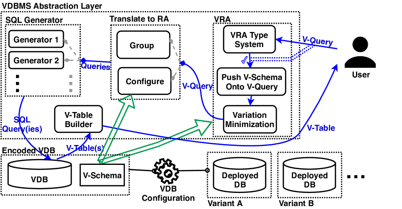
Figure 7. VDBMS architecture. The dotted double-line from v-query to pushing v-schema module indicates the dependency of passing the v-query to this module only if it is well-typed. The dashed gray arrows with diamond heads demonstrate an option for the flow of inputs. The blue filled arrows track the data flow, the green hollow arrows indicate an input to a module.

6.1. Implementing A Variational Entity

Recognizing that all entities in VDBMS including tables, schemas, VDBs, and queries are variational, we implement the variational shared interface to consists of all methods that variational objects share. As illustrated through § 4 and § 5.1.1, a variational object has two main methods: 1) configure: given a variational object and a configuration returns the non-variational object variant, i.e., configure is a function $\mathbb{X}\llbracket.\rrbracket_{c}:\mathbf{O}\to\mathbf{C}\to\underline{\mathbf{O}}$ and 2) group: given a variational object returns groups of annotated non-variational objects with a feature expression where the feature expression describes the group of configurations where the object is present, i.e., group is a function $\mathcal{G}\left({.}\right):\mathbf{O}\to\ddot{\underline{\mathbf{O}}}$. Remember, annotated objects are still variational, however, the group method removes any kinds of variability in a variational object and re-introduces variability only by annotating non-variational objects. Examples of configuring and grouping v-queries are given in § 5.1.1.

6.1.1. Configuring A Variational Entity

Conceptually, a variational entity represents many different non-variational entities that can be obtained by configuration, as shown already for v-schema, VDB, and v-query. Hence, we define the configure method for all instances of the variational interface.

6.1.2. Grouping A Variational Entity

In essence, while configuring a variational entity may generate duplicate non-variational entities, grouping a variational entity gathers the unique non-variational entities and annotates them with a feature expression that represent the group of configurations where the non-variational entity is the result of configuring the variational entity with that configuration, i.e., it moves the variation to the top level of a variational entity. Hence, a variational entity $x$ can be grouped into multiple non-variational entities annotated with a feature expression $e$, where $e$  represents the set (group) of configurations $\mathbf{C}$ s.t. $\forall c\in\mathbf{C}:\mathbb{E}\llbracket e\rrbracket_{c}=\textrm{\small{true}}$. Thus, we define the group method for the variational interface and formulate it for the variational entity $x$ as: $\mathcal{G}\left({x}\right)=\{{\underline{x}}^{e}\hskip 6.45831pt|\hskip 6.45831pt\forall c\in\mathbf{C}:\mathbb{E}\llbracket e\rrbracket_{c}=\textrm{\small{true}},\mathbb{X}\llbracket x\rrbracket_{c}=\underline{x}\}$. As the formulation of grouping indicates, we can generate the group method for a variational entity once we have instantiated its configure method, i.e., grouping is the extensional view of the configuration method. However, this would be rather slow, hence, we define the group methods for individual instances of the variational interface in a more optimized manner. E.g., Figure 4 defines grouping of v-queries and § 5.1.1 provides an example of it.

6.2. SQL Generator

Independent from the approach used to translate a v-query to a list of RA queries, to run the v-query on the underlying VDB we need to generate SQL queries from RA queries. The SQL generator module achieves this by implementing two approaches: 1) generate an SQL query per RA query which is rather a straight forward translation and 2) generate an SQL query per a set of RA queries that requires generating a unified variational attribute set for all the RA queries, adjusting the projected attributes for each RA query to conform to the unified variational attribute set by nullifying the attributes that do not exist in the original RA query, and then unioning all the generated SQL queries resulting in one SQL query. SQL queries are generated w.r.t. SQL engine’s type system, e.g., a generated query has renaming for derived subqueries even if the RA query does not. For performance purposes, we use common table expressions (CTEs) to store temporary result and reuse them in generated SQL queries.

7. Experiments and Discussion

In this section, we discuss two real world use cases of variational databases: 1) Enron email use case from SPL and 2) employee use case from schema evolution) We explain how we generated their VDBs and the set of v-queries we used for our experiments. We then state different approaches that VDBMS provides for evaluating a v-query and the result of our experiments in § 7.3. We finally conclude this section by a comprehensive discussion on benefits and shortcomings of VDBMS compared to current practices.

7.1. Generating VDB

As mentioned in § 6, VDBs are the input of VDBMS and since there are no tools to generate them, we manually generated the Enron email and employee VDBs from their two real world database variants.

Enron email VDB:

Employee VDB:

7.2. Experimental Queries

For performance purposes, we define two factors: 1) number of variants, the number of relational queries created from configuring a v-query and 2) number of variations, the number of relational queries created from grouping a v-query. To evaluate VDBMS using our two use cases, we consider a comprehensive set of queries for each VDB.

Enron email query set:

Employee query set:

7.3. Approaches and Experiments

There are four different SQL queries generated from an input set of RA queries by combining the approaches and optimizations. We use different generators to simulate current approaches used to manage variability within a context as well as comparing these methods with each other. The generated SQL queries need to be independent from the underlying DBMS that stores the VDB. Hence, the SQL generator module has a submodule that prints generated SQL queries for each DBMS engine.

7.4. Discussion

8. Related Work

We now survey works that address some kinds of variability in databases.

Variational Research:

Schema Evolution:

Database Versioning:

SPL and SPL evolution:

9. Conclusion and Future Work

Appendix A Feature Expression

Semantics of feature expressions:

$$\mathbb{E}\llbracket.\rrbracket :\mathbf{E}\to\mathbf{C}\to\mathbf{B}$$

$$\mathbb{E}\llbracket b\rrbracket_{c} =b$$

$$\mathbb{E}\llbracket f\rrbracket_{c} =c\ f$$

$$\mathbb{E}\llbracket\neg f\rrbracket_{c} =\neg\mathbb{E}\llbracket f\rrbracket_{c}$$

$$\mathbb{E}\llbracket{e}_{1}\wedge{e}_{2}\rrbracket_{c} =\mathbb{E}\llbracket e_{1}\rrbracket_{c}\wedge\mathbb{E}\llbracket e_{2}\rrbracket_{c}$$

$$\mathbb{E}\llbracket{e}_{1}\vee{e}_{2}\rrbracket_{c} =\mathbb{E}\llbracket e_{1}\rrbracket_{c}\vee\mathbb{E}\llbracket e_{2}\rrbracket_{c}$$

Functions over feature expressions:

$$\mathit{sat},\mathit{taut} :\mathbf{E}\to\mathbf{B}$$

$$\mbox{$\mathit{sat}\left(e\right)$}=\textrm{\small{true}} \textit{ iff \ }\exists c\in\mathbf{C}:\mathbb{E}\llbracket e\rrbracket_{c}=\textrm{\small{true}}$$

$$\mbox{$\mathit{taut}\left(e\right)$}=\textrm{\small{true}} \textit{ iff \ }\forall c\in\mathbf{C}:\mathbb{E}\llbracket e\rrbracket_{c}=\textrm{\small{true}}$$

Figure 8. Feature expression evaluation and functions.

Appendix B V-Condition Configuration

$$\mathbb{C}\llbracket.\rrbracket :\mathbf{\Theta}\to\mathbf{C}\to\underline{\mathbf{\Theta}}$$

$$\mathbb{C}\llbracket b\rrbracket_{c} =b$$

$$\mathbb{C}\llbracket\underline{a}\bullet k\rrbracket_{c} =\underline{a}\bullet k$$

$$\mathbb{C}\llbracket\underline{a}_{1}\bullet\underline{a}_{2}\rrbracket_{c} =\underline{a}_{1}\bullet\underline{a}_{2}$$

$$\mathbb{C}\llbracket\neg\theta\rrbracket_{c} =\neg\mathbb{C}\llbracket\theta\rrbracket_{c}$$

$$\mathbb{C}\llbracket{\theta}_{1}\vee{\theta}_{2}\rrbracket_{c} =\mathbb{C}\llbracket\theta_{1}\rrbracket_{c}\vee\mathbb{C}\llbracket\theta_{2}\rrbracket_{c}$$

$$\mathbb{C}\llbracket{\theta}_{1}\wedge{\theta}_{2}\rrbracket_{c} =\mathbb{C}\llbracket\theta_{1}\rrbracket_{c}\wedge\mathbb{C}\llbracket\theta_{2}\rrbracket_{c}$$

$$\mathbb{C}\llbracket e\langle\theta_{1},\theta_{2}\rangle\rrbracket_{c} =\begin{cases}\mathbb{C}\llbracket\theta_{1}\rrbracket_{c},&\text{ if }\mathbb{E}\llbracket e\rrbracket_{c}=\textrm{\small{true}}\\ \mathbb{C}\llbracket\theta_{2}\rrbracket_{c},&\text{ otherwise}\end{cases}$$

Figure 9. Configuration semantics of v-conditions which assumes v-conditions are well-typed.

Appendix C Configure VDB

To acquire a specific variant of a VDB instance, as illustrated in the bottom of Figure 7 and also known as VDB deployment in the context of SPL (Ataei et al., 2018), we define the configuration semantics of VDB instances. To configure a VDB instance, we configure its v-schema and v-tables, introduced in Appendix C.1 and Appendix C.2, respectively.

C.1. Configure V-Schema

To configure a VDB, its v-schema needs to be configured as well. V-schema configuration is a function that takes a v-schema and a configuration and it returns the plain relational schema variant corresponding to the configuration. Figure 10 defines the configuration semantics for v-schema and its elements, including variational attribute list and relation schemas.

Variational Attribute Set Configuration:

$$\mbox{$\mathbb{A}\llbracket.\rrbracket$}:\mathbf{A}\to\mathbf{C}\to\underline{\mathbf{A}}$$

$$\mathbb{A}\llbracket{a}^{e}\rrbracket_{c} = \begin{cases}\underline{a},\textrm{if\ }\mathbb{E}\llbracket e\wedge pc\left(rel\left(a\right)\right)\rrbracket_{c}=\textrm{\small{true}}\\ \varepsilon,\textrm{otherwise}\end{cases}$$

$$\mathbb{A}\llbracket{a}^{e},A\rrbracket_{c} = \mbox{$\mathbb{A}\llbracket{a}^{e}\rrbracket_{c}$},\mathbb{A}\llbracket A\rrbracket_{c}$$

$$\mathbb{A}\llbracket\varepsilon\rrbracket_{c} = \varepsilon$$

V-Relation Configuration:

$$\mbox{$\mathbb{R}\llbracket.\rrbracket$}:\mathbf{S}\to\mathbf{C}\to\underline{\mathbf{S}}$$

$$\mbox{$\mathbb{R}\llbracket{r}\left({A}\right)^{e}\rrbracket_{c}$}=\begin{cases}\underline{r}\left(\mathbb{A}\llbracket A\rrbracket_{c}\right),\textrm{if\ }\mathbb{E}\llbracket e\rrbracket_{c}=\textrm{\small{true}}\\ \varepsilon,\textrm{otherwise}\end{cases}$$

V-Schema Configuration:

$$\mbox{$\mathbb{S}\llbracket.\rrbracket$}:\mathbf{S}\to\mathbf{C}\to\underline{\mathbf{S}}$$

$$\mathbb{S}\llbracket{\{{r_{1}}\left({A_{1}}\right)^{e_{1}},\ldots,{r_{n}}\left({A_{n}}\right)^{e_{n}}\}}^{m}\rrbracket_{c}$$

$$\hskip 8.5359pt=\begin{cases}\{\mathbb{R}\llbracket r_{1}\left(A_{1}\right)^{e_{1}\wedge m}\rrbracket_{c},\ldots,\mathbb{R}\llbracket r_{n}\left(A_{n}\right)^{e_{n}\wedge m}\rrbracket_{c}\},\text{ if }\mathbb{E}\llbracket m\rrbracket_{c}=\textrm{\small{true}}\\ \{\ \},\qquad\qquad\qquad\qquad\qquad\quad\text{ otherwise}\end{cases}$$

Figure 10. Configuration of variational set of attributes, v-relations, and v-schema. $\varepsilon$ denotes both an empty variational set of attributes and a non-existence relation. Note that the feature model and relation presence condition are passed all the way to attributes due to the hierarchal structure of presence conditions within a v-schema.

C.2. Configure V-Table

To configure a VDB, its content, i.e., tables, need to be configured too. The relation schemas of tables have been configured by the configuration of v-schema, hence, the configuration of v-table needs to only configure tuples. I.e., v-table configuration already knows the schema of the relation (i.e., its attributes), hence, it does not need to check if a value should be included or not. Figure 11 defines v-table configuration semantics.

V-Tuple Configuration:

$$\mbox{$\mathbb{U}\llbracket.\rrbracket$}:U\to\mathbf{C}\to\underline{U}$$

$$\mbox{$\mathbb{U}\llbracket\left({v_{1},\ldots,v_{k},e_{u}}\right)\rrbracket_{c}$}=\left(\mathbb{V}\llbracket v_{1}\rrbracket_{c},\ldots,\mathbb{V}\llbracket v_{k}\rrbracket_{c}\right)$$

$$\textit{ where }\forall 1\leq i\leq k:\mathbb{V}\llbracket v_{i}\rrbracket_{c}=\begin{cases}v_{i},\textrm{if\ }\mathbb{E}\llbracket pc\left(att\left(v_{i}\right)\right)\wedge e_{u}\rrbracket_{c}=\textrm{\small{true}}\\ \varepsilon,\textrm{otherwise}\end{cases}$$

V-Table Configuration:

$$\mbox{$\mathbb{T}\llbracket.\rrbracket$}:\mathbf{R}\to\mathbf{C}\to\underline{\mathbf{R}}$$

$$\mbox{$\mathbb{T}\llbracket\{u_{1},\ldots,u_{n}\}\rrbracket_{c}$}=\{\mathbb{U}\llbracket u_{1}\rrbracket_{c},\ldots,\mathbb{U}\llbracket u_{n}\rrbracket_{c}\}$$

VDB Instance Configuration:

$$\mbox{$\mathbb{I}\llbracket.\rrbracket$}:\mathbf{I}\to\mathbf{C}\to\underline{\mathbf{I}}$$

$$\mbox{$\mathbb{I}\llbracket{\{U_{1},\ldots,U_{l}\}}^{m}\rrbracket_{c}$}=\{\mathbb{T}\llbracket U_{1}\rrbracket_{c},\ldots,\mathbb{T}\llbracket U_{l}\rrbracket_{c}\}$$

Figure 11. V-tuple, v-table, and VDB instance configuration. $\varepsilon$ denotes a non-existence value.

References

- (1)
- (2001) 2001. Software Product Lines: Practices and Patterns. Addison-Wesley Longman Publishing Co., Inc., Boston, MA, USA.
- Ataei et al. (2017) Parisa Ataei, Arash Termehchy, and Eric Walkingshaw. 2017. Variational databases. In Proceedings of The 16th International Symposium on Database Programming Languages, DBPL 2017, Munich, Germany, September 1, 2017. 11:1–11:4. https://doi.org/10.1145/3122831.3122839
- Ataei et al. (2018) Parisa Ataei, Arash Termehchy, and Eric Walkingshaw. 2018. Managing Structurally Heterogeneous Databases in Software Product Lines. In Heterogeneous Data Management, Polystores, and Analytics for Healthcare - VLDB 2018 Workshops, Poly and DMAH, Rio de Janeiro, Brazil, August 31, 2018, Revised Selected Papers. 68–77. https://doi.org/10.1007/978-3-030-14177-6_6
- Botterweck and Pleuss (2014) Goetz Botterweck and Andreas Pleuss. 2014. Evolution of Software Product Lines. Springer Berlin Heidelberg, Berlin, Heidelberg, 265–295. https://doi.org/10.1007/978-3-642-45398-4_9
- Curino et al. (2008) Carlo A. Curino, Hyun J. Moon, and Carlo Zaniolo. 2008. Graceful Database Schema Evolution: The PRISM Workbench. Proc. VLDB Endow. 1, 1 (Aug. 2008), 761–772. https://doi.org/10.14778/1453856.1453939
- Doan et al. (2012) AnHai Doan, Alon Halevy, and Zachary Ives. 2012. Principles of Data Integration (1st ed.). Morgan Kaufmann Publishers Inc., San Francisco, CA, USA.
- Erwig and Walkingshaw (2011) Martin Erwig and Eric Walkingshaw. 2011. The Choice Calculus: A Representation for Software Variation. ACM Trans. on Software Engineering and Methodology (TOSEM) 21, 1 (2011), 6:1–6:27.
- Erwig et al. (2013) Martin Erwig, Eric Walkingshaw, and Sheng Chen. 2013. An Abstract Representation of Variational Graphs. In Int. Work. on Feature-Oriented Software Development (FOSD). 25–32.
- Herrmann et al. (2015) Kai Herrmann, Jan Reimann, Hannes Voigt, Birgit Demuth, Stefan Fromm, Robert Stelzmann, and Wolfgang Lehner. 2015. Database Evolution for Software Product Lines. In DATA.
- Liebig et al. (2010) Jörg Liebig, Sven Apel, Christian Lengauer, Christian Kästner, and Michael Schulze. 2010. An Analysis of the Variability in Forty Preprocessor-based Software Product Lines. 105–114. https://doi.org/10.1145/1806799.1806819
- Moon et al. (2008) Hyun J. Moon, Carlo A. Curino, Alin Deutsch, Chien-Yi Hou, and Carlo Zaniolo. 2008. Managing and Querying Transaction-time Databases Under Schema Evolution. Proc. VLDB Endow. 1, 1 (Aug. 2008), 882–895. https://doi.org/10.14778/1453856.1453952
- Stonebraker et al. (2016) Micheal Stonebraker, Dong Deng, and Micheal L. Brodie. 2016. Database Decay and How to Avoid It. In Big Data (Big Data), 2016 IEEE International Conference. IEEE. https://doi.org/10.1109/BigData.2016.7840584
- Velegrakis et al. (2003) Yannis Velegrakis, Renée J. Miller, and Lucian Popa. 2003. - Mapping Adaptation under Evolving Schemas. In Proceedings 2003 VLDB Conference, Johann-Christoph Freytag, Peter Lockemann, Serge Abiteboul, Michael Carey, Patricia Selinger, and Andreas Heuer (Eds.). Morgan Kaufmann, San Francisco, 584 – 595. https://doi.org/10.1016/B978-012722442-8/50058-6
- Walkingshaw (2013) Eric Walkingshaw. 2013. The Choice Calculus: A Formal Language of Variation. In PhD Dissertation. Oregon State University. http://hdl.handle.net/1957/40652.
- Walkingshaw et al. (2014) Eric Walkingshaw, Christian Kästner, Martin Erwig, Sven Apel, and Eric Bodden. 2014. Variational Data Structures: Exploring Trade-Offs in Computing with Variability. In ACM SIGPLAN Symp. on New Ideas in Programming and Reflections on Software (Onward!). 213–226.
- Yu and Popa (2005) Cong Yu and Lucian Popa. 2005. Semantic Adaptation of Schema Mappings when Schemas Evolve. In Proceedings of the 31st International Conference on Very Large Data Bases (VLDB ’05). VLDB Endowment, 1006–1017. http://dl.acm.org/citation.cfm?id=1083592.1083708