Efficient Global String Kernel with Random Features:
Beyond Counting Substructures

Abstract.

Analysis of large-scale sequential data has been one of the most crucial tasks in areas such as bioinformatics, text, and audio mining. Existing string kernels, however, either (i) rely on local features of short substructures in the string, which hardly capture long discriminative patterns, (ii) sum over too many substructures, such as all possible subsequences, which leads to diagonal dominance of the kernel matrix, or (iii) rely on non-positive-definite similarity measures derived from the edit distance. Furthermore, while there have been works addressing the computational challenge with respect to the length of string, most of them still experience quadratic complexity in terms of the number of training samples when used in a kernel-based classifier. In this paper, we present a new class of global string kernels that aims to (i) discover global properties hidden in the strings through global alignments, (ii) maintain positive-definiteness of the kernel, without introducing a diagonal dominant kernel matrix, and (iii) have a training cost linear with respect to not only the length of the string but also the number of training string samples. To this end, the proposed kernels are explicitly defined through a series of different random feature maps, each corresponding to a distribution of random strings. We show that kernels defined this way are always positive-definite, and exhibit computational benefits as they always produce Random String Embeddings (RSE) that can be directly used in any linear classification models. Our extensive experiments on nine benchmark datasets corroborate that RSE achieves better or comparable accuracy in comparison to state-of-the-art baselines, especially with the strings of longer lengths. In addition, we empirically show that RSE scales linearly with the increase of the number and the length of string.

1. Introduction

String classification is a core learning task and has drawn considerable interests in many applications such as computational biology (Leslie et al., 2001; Kuksa et al., 2009), text categorization (Lodhi et al., 2002; Wu et al., 2018c), and music classification (Farhan et al., 2017). One of the key challenges in string data lies in the fact that there is no explicit feature in sequences. A kernel function corresponding to a high dimensional feature space has been proven to be an effective method for sequence classification (Xing et al., 2010; Leslie et al., 2004).

Over the last two decades, a number of string kernel methods (Cristianini et al., 2000; Leslie et al., 2001; Smola and Vishwanathan, 2003; Leslie et al., 2003; Kuang et al., 2005; Leslie et al., 2004) have been proposed, among which the $k$-spectrum kernel (Leslie et al., 2001), $(k,m)$-mismatch kernel and its fruitful variants (Leslie et al., 2003; Leslie and Kuang, 2004; Leslie et al., 2004) have gained much popularity due to its strong empirical performance. These kernels decompose the original strings into sub-structures, i.e., a short k-length subsequence as a $k$-mer, and then count the occurrences of $k$-mers (with up to $m$ mismatches) in the original sequence to define a feature map and its associated string kernels. However, these methods only consider the local properties of the short substructures in the strings, failing to capture the global properties highly related to some discriminative features of strings, i.e., relatively long subsequences.

When considering larger $k$ and $m$, the size of the feature map grows exponentially, leading to serious diagonal dominance problem due to high-dimension sparse feature vector (Greene and Cunningham, 2006; Weston et al., 2003). More importantly, the high computational cost for computing kernel matrix renders them only applicable to small values of $k$, $m$, and small data size. Recently, a thread of research has made the valid attempts to improve the computation for each entry of the kernel matrix (Kuksa et al., 2009; Farhan et al., 2017). However, these new techniques only solve the scalability issue in terms of the length of strings and the size of alphabet but not the kernel matrix construction that still has quadratic complexity in the number of strings. In addition, these approximation methods still inherit the issues of these ”local” kernels, ignoring global structures of the strings, especially for these of long lengths.

Another family of research (Waterman et al., 1991; Watkins, 1999; Gordon et al., 2003; Saigo et al., 2004; Haasdonk and Bahlmann, 2004; Cortes et al., 2004; Neuhaus and Bunke, 2006) utilizes a distance function to compute the similarity between a pair of strings through the global or local alignment measure (Needleman and Wunsch, 1970; Smith and Waterman, 1981). These string alignment kernels are defined resorting to the learning methodology of R-convolution (Haussler, 1999), which is a framework for computing the kernels between discrete objects. The key idea is to recursively decompose structured objects into sub-structures and compute their global/local alignments to derive a feature map. However, the common issue that these string alignment kernels have to address is how to preserve the property of being a valid positive-definite (p.d.) kernel (Schölkopf et al., 2004). Interestingly, both approaches (Gordon et al., 2003; Saigo et al., 2004) proposed to sum up all possible alignments to yield a p.d. kernel, which unfortunately suffers the diagonal dominance problem, leading to bad generealization capability. Therefore, some treatments have to be made in order to repair the issues, e.g. taking the logarithm of the diagonal, which in turns breaks the positive definiteness. Another important limitation of these approaches is their high computation costs, with the quadratic complexity in terms of both the number and the length of strings.

In this paper, we present a new family of string kernels that aims to: (i) discover global properties hidden in the strings through global alignments, (ii) maintain positive-definiteness of the kernel, without introducing a diagonal dominant kernel matrix, and (iii) have a training cost linear with respect to not only the length of the string but also the number of training string samples.

To this end, our proposed global string kernels take into account the global properties of strings through the global-alignment based edit distance such as Levenshtein distance (Yujian and Bo, 2007). In addition, the proposed kernels are explicitly defined through feature embedding given by a distribution of random strings. The resulting kernel is not only a truly p.d. string kernel without suffering from diagonal dominance but also naturally produces Random String Embeddings (RSE) by utilizing Random Features (RF) approximations. We further design four different sampling strategies to generate an expressive RSE, which is the key leading to state-of-the-art performance in string classification. Owing to the short length of random strings, we reduce the computational complexity of RSE from quadratic to linear both in the number of strings and the length of string. We also show the uniform convergence of RSE to a p.d. kernel that is not shift-invariant for string of bounded length by non-trivially extending conventional RF analysis (Rahimi and Recht, 2008).

Our extensive experiments on nine benchmark datasets corroborate that RSE achieves better or comparable accuracy in comparison to state-of-the-art baselines, especially with the strings of longer lengths. In addition, RSE scales linearly with the increase of the number and the length of strings. Our code is available at https://github.com/IBM/RandomStringEmbeddings.

2. Existing String Kernels and Conventional Random Features

In this section, we first introduce existing string kernels and its several important issues that impair their effectiveness and efficiency. We next discuss the conventional Random Features for scaling up large-scale kernel machines and further illustrate several challenges why the conventional Random Features cannot be directly applied to existing string kernels.

2.1. Existing String Kernels

We discuss existing approaches of defining string kernels and also three issues that have been haunting existing string kernels for a long time: (i) diagonal dominance; (ii) non-positive definite; (iii) scalability issue for large-scale string kernels

2.1.1. String Kernel by Counting Substructures

We consider a family of string kernels most commonly used in the literature, where the kernel $k(\boldsymbol{x},\boldsymbol{y})$ between two strings $\boldsymbol{x},\boldsymbol{y}\in\mathcal{X}$ is computed by counting the number of shared substructures between $\boldsymbol{x}$, $\boldsymbol{y}$. Let $S$ denote the set of indices of a particular substructure in $\boldsymbol{x}$ (e.g. subsequence, substring, or single character), and $\mathcal{S}(\boldsymbol{x})$ be the set of all possible such set of indices. Furthermore, let $\mathcal{U}$ be all possible values of such substructure. Then a family of string kernels can be defined as

(1) $$k(\boldsymbol{x},\boldsymbol{y}):=\sum_{u\in\mathcal{U}}\phi_{u}(\boldsymbol{x})\phi_{u}(\boldsymbol{y}),\text{where}\;\phi_{u}(\boldsymbol{x})=\sum_{S\in\mathcal{S}}1_{u}(\boldsymbol{x}[S])\gamma(S)$$

and $1_{u}(\boldsymbol{x}[S])$ is the number of substructures in $\boldsymbol{x}$ of value $u$, weighted by $\gamma(S)$, which reduces the count according to the properties of $S$, such as length. For example, in a vanilla text kernel, $\mathcal{S}$ denotes word positions in a document $\boldsymbol{x}$ and $\mathcal{U}$ denotes the vocabulary set (with $\gamma(S)=1$). To take string structure into consideration, the gappy n-gram (Lodhi et al., 2002) considers $\mathcal{S}(\boldsymbol{x})$ as the set of all possible subsequences in a string $\boldsymbol{x}$ of length $k$, with $\gamma(S)=\exp(-\ell(S))$ being a weight exponentially decayed function in the length of $S$ to penalize subsequences of large number of insertions and deletions. While the number of possible subsequences in a string is exponential in the string length, there exist dynamic-programming-based algorithms that could compute the kernel in Equation (1) in time $O(k|\boldsymbol{x}||\boldsymbol{y}|)$ (Lodhi et al., 2002). Similarly, or more complex, substructures were employed in the convolution kernels (Haussler, 1999) and (Watkins, 1999). Both of them have quadratic complexity w.r.t. the string length, which is too expensive for problems of long strings.

To circumvent this issue, Leslie et al. proposed the $k$-spectrum kernel (or gap-free $k$-gram kernel) (Leslie et al., 2001), which only requires a computation time $O(k(|\boldsymbol{x}|+|\boldsymbol{y}|))$ linear to the string length, by taking $\mathcal{S}$ as all substrings (without gap) of length $k$, where they could be even further improved to $O(|\boldsymbol{x}|+|\boldsymbol{y}|)$ (Smola and Vishwanathan, 2003). While this significantly increases computational efficiency, the no gap assumption is too strong in practice. Therefore, the $(k,m)$-mismatch kernel (Leslie et al., 2003; Leslie et al., 2004) is more widely used, which considers $1_{u}(\boldsymbol{x}[S])=1$ not only when the $k$-mer $\boldsymbol{x}[S]$ exactly matches $u$ but also when they mismatch by no more than $m$ characters. The algorithm has a computational burden of $O(k^{m+1}|\Sigma|^{m}(|\boldsymbol{x}|+|\boldsymbol{y}|))$ and a number of more recent works improved it to $O(m^{3}+2^{k}(|\boldsymbol{x}|+|\boldsymbol{y}|))$ in the exact case and even faster in the approximate case (Kuksa et al., 2009; Farhan et al., 2017).

One significant issue regarding substructure-counting kernel is the diagonally dominant problem, where the diagonal elements of a kernel Gram matrix is significantly (often orders-of-magnitude) larger than the off-diagonal elements, yielding an almost identity kernel matrix that Support Vector Machine (SVM) does not perform well on (Weston et al., 2003; Greene and Cunningham, 2006). This is because a string always shares a large number of common substructures with itself, and the issue is more serious for the problems summing over more substructures in $\mathcal{S}$.

2.1.2. Edit-Distance Substitution Kernel

Another commonly used approach is to define string kernels by exploiting the edit distance (e.g. Levenshtein distance). With a slight abuse of notation, let $d(i,j)$ denote the Levenshtein distance (LD) between two substrings $d(\boldsymbol{x}[1:i],\boldsymbol{y}[1:j])$. The distance can be recursively defined as follows.

(2) $$d(i,j)=\left\{\begin{array}[]{ll}\max\{i,j\},\ \ \ i=0\;\text{or}\;j=0\\ \min\left\{\begin{array}[]{l}d(i-1,j)+1,\\ d(i,j-1)+1,\\ d(i-1,j-1)+1_{\boldsymbol{x}[i]\neq\boldsymbol{y}[j]}\end{array}\right\},&\ o.w.\end{array}\right.$$

Essentially, the distance (2) finds the minimum number of edits (i.e. insertion, deletion, and substitution) required to transform $\boldsymbol{x}$ into $\boldsymbol{y}$. The distance measure is known as a metric, that is, it satisfies (i) $d(\boldsymbol{x},\boldsymbol{y})\geq 0$, (ii) $d(\boldsymbol{x},\boldsymbol{y})=d(\boldsymbol{y},\boldsymbol{x})$, (iii) $d(\boldsymbol{x},\boldsymbol{y})=0$ $\iff$ $\boldsymbol{x}=\boldsymbol{y}$ and (iv) $d(\boldsymbol{x},\boldsymbol{y})+d(\boldsymbol{y},\boldsymbol{z})\geq d(\boldsymbol{x},\boldsymbol{z})$.

Then the distance-substitution kernel (Haasdonk and Bahlmann, 2004) replaces the Euclidean distance in a typical kernel function by a new distance $d(\boldsymbol{x},\boldsymbol{y})$. For example, for Gaussian and Laplacian RBF kernels, the distance substitution leads to

(3) $$k_{Gauss}(\boldsymbol{x},\boldsymbol{y}):=\exp(-\gamma d(\boldsymbol{x},\boldsymbol{y})^{2})$$

(4) $$k_{Lap}(\boldsymbol{x},\boldsymbol{y}):=\exp(-\gamma d(\boldsymbol{x},\boldsymbol{y})).$$

The kernels, however, are not positive-definite for the case of edit distance (Neuhaus and Bunke, 2006). This implies that the use of string kernels (3), (4) in a kernel method, such as SVM, does not correspond to a loss minimization problem, and the numerical procedure can not guarantee convergence to an optimal solution since the non-p.d. kernel matrix yields a non-convex optimization problem. Despite being invalid, this type of kernels is still being used in practice (Neuhaus and Bunke, 2006; Loosli et al., 2016).

2.2. Conventional Random Features for Scaling Up Kernel Machine

As we discussed in the previous sections, while there have been works addressing the computational challenge with respect to the length of string or the size of the alphabet, all of exiting string kernels still have quadratic complexity in terms of the number of strings when computing the kernel matrix for string classification.

Independently, over the last decade, there has been growing interests in the development of various low-rank kernel approximation techniques for scaling up large-scale kernel machines such as Nystrom method (Williams and Seeger, 2001), Random Features method (Rahimi and Recht, 2008), and other hybrid kernel approximation methods (Si et al., 2017). Among them, RF method has attracted considerable interests due to easy implementation and fast execution time (Rahimi and Recht, 2008; Wu et al., 2016, 2018a), and has been widely applied to various applications such as speech recognition and computer vision (Huang et al., 2014; Chen et al., 2016). In particular, unlike other approaches that approximates kernel matrix, RF method approximates the kernel function directly via sampling from an explicit feature map. Therefore, these random features, combined with very simple linear learning techniques, can effectively reduce the computational complexity of the exact kernel matrix from quadratic to linear in terms of the number of training samples.

Despite the great success the conventional RF method has achieved, there are three key challenges in applying this technique to existing string kernels introduced in the previous section. First, the conventional RF methods are designed for the kernel machines that only take the fix-length vectors. Thus, it is not clear how to extend this technique to the string kernels that take variable-length strings. Second, all conventional RF methods require a user-defined kernel as inputs and then derive the corresponding random feature map. For given kernel functions like Gaussian or Laplacian RBF kernels, it might be easy to derive random feature maps, i.e. Gaussian distribution and Gamma distribution. However, it is highly non-trivial how to derive a random feature map for a string kernel defined as in Equations (1), (3), and (4). Finally, the theoretical foundation to guarantee the inner product of two transformed points approximating the exact kernel is that the kernel must be shift-invariant and positive-definite. This assumption about the kernel is hard to hold for most of string kernels since existing string kernels are not a shift-invariant kernel (Wu et al., 2018b).

In this work, instead of using Random Features to approximate a pre-defined kernel function, we overcome all these aforementioned issues by generalizing Random Features to develop a new family of efficient and effective string kernels that not only are positive-definite but also reduce the computational complexity from quadratic to linear in both the number and the length of strings. Note that, our approach is different from a recent work (Wu et al., 2018b) on distance kernel learning that mainly focuses on theoretical analysis of these kernels on structured data like time-series (Wu et al., 2018d) and text (Wu et al., 2018c). Instead, we focus on developing empirical methods that could often outperform or are highly competitive to other state-of-the-art approaches, including kernel based and Recurrent Neural Networks based methods, as we will show in our experiments.

3. From Edit Distance to String Kernel

In this section, we first introduce a family of string kernels that utilize the global alignment measure, i.e. Edit Distance (or Levenshtein distance), to construct a kernel while establishing its positive definiteness. Then we further discuss how to perform efficient computation of the proposed string kernels by generating the kernel approximation through Random Features that we refer as Random String Embeddings. Finally, we show the uniform convergence of RSE to a p.d. kernel that is not shift-invariant.

3.1. Global String Kernel

Suppose we are interested in strings of bounded length $L$, that is, $\mathcal{X}\in\Sigma^{L}$. Let $\Omega\in\Sigma^{L}$ also be a domain of strings and $p(\boldsymbol{\omega}):\Omega\rightarrow\mathbb{R}$ be a probability distribution over a collection of random strings $\boldsymbol{\omega}\in\Omega$. The proposed kernel is defined as

(5) $$k(\boldsymbol{x},\boldsymbol{y}):=\int_{\boldsymbol{\omega}\in\Omega}p(\boldsymbol{\omega})\phi_{\boldsymbol{\omega}}(\boldsymbol{x})\phi_{\boldsymbol{\omega}}(\boldsymbol{y})d\boldsymbol{\omega},$$

where $\phi_{\boldsymbol{\omega}}(\boldsymbol{x})$ could be set directly to the distance

(6) $$\phi_{\boldsymbol{\omega}}(\boldsymbol{x}):=d(\boldsymbol{x},\boldsymbol{\omega})$$

or be converted into a similarity measure via the transformation

(7) $$\phi_{\boldsymbol{\omega}}(\boldsymbol{x}):=\exp(-\gamma d(\boldsymbol{x},\boldsymbol{\omega})).$$

In the former case, it could be illustrated as some form of the distance substitution kernel but using a distribution of random strings instead of the original strings. In the latter case, it could be interpreted as a soft distance substitution kernel. Instead of substituting distance into the function like (4), it substitutes a soft version of the form

(8) $$k(\boldsymbol{x},\boldsymbol{y})=\exp\left(-\gamma\mathit{softmin}_{p(\boldsymbol{\omega})}\{d(\boldsymbol{x},\boldsymbol{\omega})+d(\boldsymbol{\omega},\boldsymbol{y})\}\right)$$

where

$$\mathit{softmin}_{p(\boldsymbol{\omega})}(f(\boldsymbol{\omega})):=-\frac{1}{\gamma}\log\int p(\boldsymbol{\omega})e^{-\gamma f(\boldsymbol{\omega})}d\boldsymbol{\omega}.$$

Suppose $\Omega$ only contains strings of non-zero probability (i.e. $p(\boldsymbol{\omega})>0$). Comparing (8) to the distance-substitution kernel (4), we notice that

$$\mathit{softmin}_{p(\boldsymbol{\omega})}(f(\boldsymbol{\omega}))\rightarrow\min_{\boldsymbol{\omega}\in\Omega}\;f(\boldsymbol{\omega})$$

as $\gamma\rightarrow\infty$. As long as $\mathcal{X}\subseteq\Omega$ and the global alignment measure (i.e. Levenshtein distance) satisfies the triangular inequality (Levenshtein, 1966), then we have

$$\min_{\boldsymbol{\omega}\in\Omega}d(\boldsymbol{x},\boldsymbol{\omega})+d(\boldsymbol{y},\boldsymbol{\omega})=d(\boldsymbol{x},\boldsymbol{y}),$$

and therefore,

$$k(\boldsymbol{x},\boldsymbol{y})\rightarrow\exp(-\gamma d(\boldsymbol{x},\boldsymbol{y}))$$

as $\gamma\rightarrow\infty$, which relates our kernel (8) to the distance-substitution kernel (4) in the limiting case. However, note that our kernel (8) is always positive definite by its definition (5) since

(9) $$\begin{split}&\int_{\boldsymbol{x}}\int_{\boldsymbol{y}}\int_{\boldsymbol{\omega}\in\Omega}p(\boldsymbol{\omega})\phi_{\boldsymbol{\omega}}(\boldsymbol{x})\phi_{\boldsymbol{\omega}}(\boldsymbol{y})d\boldsymbol{\omega}\boldsymbol{x}\boldsymbol{y}\\ &=\int_{\boldsymbol{\omega}\in\Omega}p(\boldsymbol{\omega})\left(\int_{\boldsymbol{x}}\phi_{\boldsymbol{\omega}}(\boldsymbol{x})d\boldsymbol{x}\right)\left(\int_{\boldsymbol{y}}\phi_{\boldsymbol{\omega}}(\boldsymbol{y})d\boldsymbol{y}\right)d\boldsymbol{\omega}\geq 0\end{split}$$

3.2. Random String Embedding

Efficient Computation of RSE. Although the kernels (6) and (7) are clearly defined and easy to understand, it is hard to derive a simple analytic form of solution. Fortunately, we can easily utilize the RF approximations for the exact kernel,

(10) $$\hat{k}_{R}(\boldsymbol{x},\boldsymbol{y})\ \approx\ \ \big{\langle}Z(\boldsymbol{x}),Z(\boldsymbol{y})\big{\rangle}=\frac{1}{R}\sum_{i=1}^{R}\big{\langle}\phi_{\boldsymbol{\omega}_{i}}(\boldsymbol{x}),\phi_{\boldsymbol{\omega}_{i}}(\boldsymbol{y})\big{\rangle}.$$

The feature vector $Z(\boldsymbol{x})$ is computed using dissimilarity measure $\phi({\{\boldsymbol{\omega}_{i}\}}_{i=1}^{R},x)$, where ${\{\boldsymbol{\omega}_{i}\}}_{i=1}^{R}$ is a set of random strings of variable length $D$ drawn from a distribution $p(\boldsymbol{\omega})$. In particular, the function $\phi$ could be any edit distance measure or converted similarity measure that consider global properties through alignments. Without loss of generality we consider Levenshtein distance (LD) as our distance measure, which has been shown to be a true distance metric (Yujian and Bo, 2007). We call our random approximation Random String Embedding (RSE), which we will show its uniform convergence to the exact kernel over all pairs of strings by non-trivially extending the conventional RF analysis in (Rahimi and Recht, 2008) to the kernel that is not shift-invariant and the inputs that are not fixed-length vectors. It is worth noting that only feature matrix $Z$ is actually computed for string classification tasks and there is no need to compute $\hat{k}_{R}(\boldsymbol{x},\boldsymbol{y})$.

Algorithm 1 Random String Embedding: An Unsupervised Feature Representation Learning for Strings

1:Input: Strings $\{x_{i}\}_{i=1}^{N},1\leq|x_{i}|\leq L$, maximum length of random strings $D_{max}$, string embedding size $R$.

2:Output: Feature matrix $Z_{N\times R}$ for input strings

3:for $j=1,\ldots,R$ do

4:   Draw $D_{j}$ uniformly from $[1,D_{max}]$.

5:   Generate random strings $\omega_{j}$ of length $D_{j}$ from Algorithm 2.

6:   Compute a feature vector $Z(:,j)=\phi_{\omega_{i}}(\{x_{i}\}_{i=1}^{N})$ using LD in (6) or soft-version LD in (7).

7:end for

8:Return feature matrix $Z(\{x_{i}\}_{i=1}^{N})=\frac{1}{\sqrt{R}}[Z(:,1:R)]$

As shown in Algorithm 1, our Random String Embedding is very simple and can be easily implemented. There are several remarks worth noting here. First, RSE is an unsupervised feature generation method for embedding strings, making it highly flexible to be combined with various learning tasks beside classification. The hyperparamter $D_{max}$ is for both the kernel (6) and the kernel (7), and the hyperparameter $\gamma$ is only for the kernel (7) using soft-version LD distance as features. One interesting way to illustrate the role of $D$ in lines 2 and 3 of Alg. 1 is to capture the longest segments of the original strings that correspond to the highly discriminative features hidden in the data. We have observed in our experiments that these long segments are particularly important for capturing the global properties of the strings of long length ($L>1000$). In practice, we have no prior knowledge about the value of $D$ and thus we sample each random string of $D$ in the range $[1,\ D_{max}]$ to yield unbiased estimation. In practice, $D$ is often a constant, typically smaller than 30. Finally, in order to learn an expressive representation, generating a set of random strings of high-quality is a necessity, which we defer to discuss in detail later.

One important aspect about our RSE embedding method stems from the fact that it scales linearly both in the number of strings and in the length of strings. Notice that a typical evaluation of LD between two data strings is $O(L^{2})$ given that two strings have roughly equal length $L$. With our RSE, we can reduce the computational cost of LD to $O(LD)$, where $D$ is treated as a constant in Algorithm 1. This is particular important when the length of the original strings are very long. In addition, most of popular existing string kernels have quadratic complexity $O(N^{2})$ in computing kernel matrix in terms of the number of strings, rendering the serious difficulty to scale to large data. In contrast, our RSE reduces this computational complexity from quadratic to linear, owing to generating an embedding matrix with $O(NR)$ instead of constructing a full kernel matrix directly. Recall that the state-of-the-art string kernels have complexity of $O(N^{2}(m^{3}+2^{k}L))$ (Farhan et al., 2017; Kuksa et al., 2009). Therefore, with our RSE method we have significantly improved the total complexity of $O(NRL)$, if we treat $D$ as a constant, which is independent of the size of alphabet $k$ and the number of mismatched characters $m$. We demonstrate the linear scalability of RSE respecting to the number of strings and the length of strings, making it a strong candidate for the method of the choice for string kernels on large data.

Algorithm 2 Sampling Strategies for Generating Random Strings

1:Input: Strings $\{x_{i}\}_{i=1}^{N}$, length of random string $D_{j}$, size of alphabet $|\Sigma|$.

2:Output: Random strings $\omega_{i}$

3:if Choose RSE(RF) then

4:   Uniformly draw number $D_{j}$ of indices $\{I_{1},I_{2},\ldots,I_{D_{j}}\}=\text{randi}(|\Sigma|,1,D_{j})$

5:   Obtain random characters from $\Sigma(\{I_{1},I_{2},\ldots,I_{D_{j}}\})$

6:   Generate random string $\omega_{i}$ by concatenating random characters

7:else if Choose RSE(RFD) then

8:   compute the discrete distribution $h(\omega)$ for each character in alphabet $\Sigma$

9:   Draw number $D_{j}$ of indices $\{I_{1},I_{2},\ldots,I_{D_{j}}\}=\text{randi}(|\Sigma|,1,D_{j})$ from data letter distribution $h(\omega)$

10:   Obtain random characters from $\Sigma(\{I_{1},I_{2},\ldots,I_{D_{j}}\})$

11:   Generate random string $\omega_{i}$ by concatenating random characters

12:else if Choose RSE(SS) then

13:   Uniformly draw string index $k=\text{randi}(1,N)$ and select the $k$-th raw string

14:   Obtain length $L_{k}$ of the $k$-th raw string and uniformly draw letter index $l=\text{randi}(1,L_{k}-D_{j}+1)$

15:   Generate random string $\omega_{i}$ from a continuous segment of $k$-th raw string starting from $l$-th letter

16:else if Choose RSE(BSS) then

17:   Uniformly draw string index $k=\text{randi}(1,N)$, select the $k$-th raw string, and obtain its length $L_{k}$

18:   Divide $k$-th raw string into $b=L_{k}/D_{j}$ blocks of sub-string

19:   Uniformly draw number of blocks that will be sampled $l=randi(1,b)$

20:   Uniformly draw block indices $\{B_{1},B_{2},\ldots,B_{l}\}=\text{randi}(b,1,l)$

21:   Generate number $l$ of random strings $\omega_{i}$ by gathering all drawn blocks of sub-strings (and remove if it has in $\{\omega_{i}\}$)

22:end if

23:Return $\omega_{i}$ for all generated random strings

Effective Random Strings Generation. The key to the effectiveness of the RSE is how to generate a set of random strings of high quality. We present four different sampling strategies to produce a rich feature space derived from both data-independent and data-dependent distributions. We summarize various sampling strategies for generating random strings in Algorithm 2.

The first sampling strategy follows the traditional RF method, where we find the distribution associated to the predefined kernel function. However, since we define the kernel function by an explicit distribution, we have flexibility to seek any existing distribution that may apply well on the data. To this end, we use uniform distribution to represent the true distribution of the characters in given specific alphabet. We call this sampling scheme RSE(RF). The second sampling strategy is a similar scheme but instead of using existing distribution we compute histograms of each character in the alphabet that appears in the data strings. The learned histogram is an biased estimate for the true probability distribution. We call this sampling scheme RSE(RFD).

The previous two sampling strategies basically consider how to generate a random string from low-level characters. Recent studies (Ionescu et al., 2017; Rudi and Rosasco, 2017) on random features have shown that a data-dependent distribution may yield better generalization error. Therefore, inspired by these findings, we also design two data-dependent sampling schemes to generate random strings. We do not use well-known representative set of method to pick the whole strings since it has been shown in (Chen et al., 2009) that this method generally leads larger generalization errors. A simple yet intuitive way to obtain random strings is to sample a segment (sub-string) of variable length from the original strings. Too long or too short sub-strings could either carry noises or insufficient information about the true data distribution. Therefore, we uniformly sample the length of random strings as before. We call this sampling scheme RSE(SS). In order to sample more random strings in one sampling period, we also divide the original string into several blocks of sub-strings and uniformly sample some number of these blocks as our random strings. Note that in this case it means that we sample multiple random strings and we do not concatenate them as one long string. This scheme leads to learn more discriminative features at the cost of more computations for running Alg. 2 once. We call this scheme RSE(BSS).

3.3. Convergence Analysis

As our kernel (5) does not have an analytic form but only a sampling approximation (10), it is crucial to ask: how many random features are required in (10) to have an accurate approximation? Does such accuracy generalize to strings beyond training data? To answer those questions, we non-trivially extending the conventional RF analysis in (Rahimi and Recht, 2008) to the proposed string kernels in Equation (5), which are not shift-invariant and take the variable-length strings. We provide the following theorem to show the uniform convergence of RSE to a p.d. string kernel over all pairs of strings.

Theorem 1.

Let $\Delta_{R}(\boldsymbol{x},\boldsymbol{y}):=\hat{k}_{R}(\boldsymbol{x},\boldsymbol{y})-k(\boldsymbol{x},\boldsymbol{y})$ be the difference between the exact kernel (5) and its random-feature approximation (10) with $R$ samples, we have the following uniform convergence:

$$P\left\{\max_{\boldsymbol{x},\boldsymbol{y}\in\mathcal{X}}|\Delta_{R}(\boldsymbol{x},\boldsymbol{y})|>t\right\}\leq 8e^{2L\log|\Sigma|-Rt^{2}/2}.$$

where $L$ is a bound on the length of strings in $\mathcal{X}$ and $|\Sigma|$ is size of the alphabet. In other words, to guarantee $|\Delta_{R}(x,y)|\leq\epsilon$ with probability at least $1-\delta$, it suffices to have

$$R=\Omega\biggl{(}\frac{L\log|\Sigma|}{\epsilon^{2}}\log(\frac{\gamma}{\epsilon})+\frac{1}{\epsilon^{2}}\log(\frac{1}{\delta})\biggr{)}.$$

Proof Sketch.

Since $E[\Delta_{R}(\boldsymbol{x},\boldsymbol{y})]=0$ and $|\Delta_{R}(\boldsymbol{x},\boldsymbol{y})|\leq 1$, from Hoefding’s inequality, we have

$$P\left\{|\Delta_{R}(\boldsymbol{x},\boldsymbol{y})|\geq t\right\}\leq 2\exp(-Rt^{2}/2)$$

and since the number of strings in $\mathcal{X}$ is bounded by $2|\Sigma|^{L}$. Through an union bound, we have

$$P\left\{\max_{\boldsymbol{x},\boldsymbol{y}\in\mathcal{X}}|\Delta_{R}(\boldsymbol{x},\boldsymbol{y})|\geq t\right\} \leq 2|\mathcal{X}|^{2}\exp(-Rt^{2}/2)$$

$$\leq 8\exp\left(2L\log|\Sigma|-Rt^{2}/2\right),$$

which leads to the result. ∎

Theorem 1 tells us that for any pair of two strings $\boldsymbol{x},\boldsymbol{y}\in\mathcal{X}$, one can guarantee a kernel approximation of error less than $\epsilon$ as long as $R\gtrapprox L\log(|\Sigma|)/\epsilon^{2}$ up to the logarithmic factor.

4. Experiments

We carry out the experiments to demonstrate the effectiveness and efficiency of the proposed method, and compare against total five state-of-the-art baselines on nine different string datasets that are widely used for testing the performance of string kernels. We implement our method in Matlab and make full use of C-MEX function for the computationally extensive component of LD.

Table 1. Statistical properties of the datasets.

Application	Name	Alphabet	Class	Train	Test	Length
Protein	ding-protein	20	27	311	369	26/967
Protein	fold	20	26	2700	1159	20/936
Protein	superfamily	20	74	3262	1398	23/1264
DNA/RNA	splice	4	3	2233	957	60
DNA/RNA	dna3-class1	4	2	3200	1373	147
DNA/RNA	dna3-class2	4	2	3620	1555	147
DNA/RNA	dna3-class3	4	2	4025	1725	147
Image	mnist-str4	4	10	60000	10000	34/198
Image	mnist-str8	8	10	60000	10000	17/99

Table 2. Comparisons among eight variants of RSE in terms of classification accuracy. Each sampling strategy combines either DF (direct LD distance as features in String Kernels (6)) or SF (soft version of LD distance as features in String Kernels (7)).

Methods	RSE(RF-DF)	RSE(RF-SF)	RSE(RFD-DF)	RSE(RFD-SF)	RSE(SS-DF)	RSE(SS-SF)	RSE(BSS-DF)	RSE(BSS-SF)
Datasets	Accu	Accu	Accu	Accu	Accu	Accu	Accu	Accu
ding-protein	52.57	51.76	51.22	49.32	48.50	53.65	51.49	52.30
fold	73.94	72.90	74.37	72.47	75.41	75.21	74.72	75.13
superfamily	74.03	73.46	74.67	70.88	77.46	77.13	74.82	75.52
splice	86.72	86.31	86.20	82.86	88.71	88.08	89.76	90.17
dna3-class1	78.29	77.20	77.85	79.46	81.64	80.84	83.39	82.66
dna3-class2	88.48	89.51	87.97	90.41	87.20	90.61	89.51	90.48
dna3-class3	75.94	78.55	72.0	70.72	70.89	72.87	78.20	78.78
mnist-str4	98.52	98.43	98.43	98.31	98.76	98.61	98.75	98.71
mnist-str8	98.45	98.48	98.39	98.31	98.54	98.51	98.50	98.53

Datasets. We apply our method on nine benchmark string datasets across different main applications including protein, DNA/RNA, and image. Table 1 summarizes the properties of datasets that are collected from the UCI Machine Learning repository (Frank and Asuncion, 2010), the LibSVM Data Collection (Chang and Lin, 2011), and partially overlapped with various string kernel references (Farhan et al., 2017; Kuksa et al., 2009). For all datasets, the size of alphabet is between 4 and 20. The number of classes range between 2 and 74. The larger number of classes typically make the classification task more challenging. One particular property associated with string data is possibly high variation in length of the strings, which exhibits mostly in the protein datasets with range between 20 and 1264. This large variation presents significant challenges to the most of methods. We divided each dataset into 70/30 train and test subsets (if there was no predefined train/test split).

Variants of RSE. We have two different global string kernels and four different random string generation methods proposed in Section 3, resulting in the total 8 different combinations of RSE. We will investigate the properties and performance of each variant in the subsequent section. Here, we list the different variants as follows: i) RSE(RF-DF): RSE(RF) with direct LD distance as features in (6); ii) RSE(RF-SF): RSE(RF) with soft version of LD distance as features in (7); iii) RSE(RFD-DF): RSE(RFD) with direct LD distance; iv) RSE(RFD-SF): RSE(RFD) with soft version of LD distance; v) RSE(SS-DF): RSE(SS) with direct LD distance; vi) RSE(SS-SF): combines the data-dependent sub-strings generated from dataset with soft LD distance; vii) RSE(BSS-DF): generates blocks of sub-strings from data-dependent distribution and uses direct LD distance; viii) RSE(BSS-SF): generates blocks of sub-strings from data-dependent distribution and uses soft-version LD distance.

Baselines. We compare our method RSE against five state-of-the-art kernel and deep learning based methods:
SSK (Kuksa et al., 2009): state-of-the-art scalable algorithms for computing exact string kernels with inexact matching - ($k,m$)-mismatch kernel.
ASK (Farhan et al., 2017): latest advancement for approximating ($k,m$)-mismatch string kernel for larger $k$ and $m$.
KSVM (Loosli et al., 2016): state-of-the-art alignment based kernels using the original (indefinite) similarity measure in the original Krein space.
LSTM (Greff et al., 2017): long short-term memory (LSTM) architecture, state-of-the-art models for sequence learning.
GRU (Cho et al., 2014): a gated recurrent unit (GRU) achieving comparable performance to LSTM (Chung et al., 2014).

For deep learning methods, we use Python Deep Learning Library Keras. Both LSTM and GRU models are trained using the Adam optimizer (Kingma and Ba, 2014), with mini-batch size 64. The learning rate is set to 0.001. We apply the dropout strategy (Srivastava et al., 2014) with a ratio of 0.5 to avoid overfitting. Gradients are clipped when their norm is bigger than 20. We set the max number of epochs 200. It is easy to see that most of Protein and DNA/RNA datasets have relatively small size of datasets, except for two image datasets. Therefore, to overcome potential over-fitting issue, we tune the number of hidden layers (using only 1 or 2) and the size of hidden state between 60 and 150. We use one-hot encoding scheme with the size of alphabet in the corresponding string data.

Table 3. Comparing RSE against other state-of-the-art methods in terms of classification accuracy and computational time (seconds). The symbol ”–” stands for either ”run out of memory” (with total 256G) or runtime greater than 36 hours.

Methods	RSE(BSS-SF)		SSK		ASK		KSVM		LSTM		GRU
Datasets	Accu	Time	Accu	Time	Accu	Time	Accu	Time	Accu	Time	Accu	Time
ding-protein	52.30	54.8	28.72	3.0	11.92	20.0	39.83	25.8	31.33	576.0	31.90	350.0
fold	75.13	289.51	46.5	85.0	48.83	1070.0	74.37	643.9	68.08	13778.0	66.83	6452.0
superfamily	75.52	469.9	44.63	140.0	44.70	257.0	69.59	1389.9	63.38	16778.0	62.81	7974.0
splice	90.17	78.4	71.26	68.0	71.57	184.0	67.29	148.8	86.94	166.0	88.39	93.2
dna3-class1	82.66	585.6	86.38	313.0	86.23	667.0	48.43	760.4	80.1	866.0	81.78	436.0
dna3-class2	90.48	432.2	82.76	475.0	82.63	916.0	46.10	991.8	83.08	1000.0	85.13	536.4
dna3-class3	78.78	1436.8	77.91	553.0	78.14	926.0	44.28	1297.2	83.36	2400.0	81.75	1389.0
mnist-str4	98.71	4287.2	–	–	–	–	–	$>\text{36 hours}$	98.63	13090.0	98.50	7542.0
mnist-str8	98.53	2010.2	–	–	–	–	96.80	859670.0	98.61	14618.0	98.45	7386.0

4.1. Comparison Among All Variants of RSE

Setup. We investigate the behaviors of eight different variants of our proposed method RSE in terms of string classification accuracy. The best values for $\gamma$ and $D_{max}$ for the length of random string were searched in the ranges [1e-5, 1] and [5, 100], respectively. Since we can generate random samples from the distribution, we can use as many as needed to achieve performance close to an exact kernel. We report the best number in the range $R=[4,\ 8192]$ (typically the larger $R$ is, the better the accuracy). We employ a linear SVM implemented using LIBLINEAR (Fan et al., 2008) on the RSE embeddings.

Results. Table 2 shows the comparison results among eight different variants of RSE for various string classification tasks. We empirically observed some interesting conclusions. First, we can see that the data-dependent sampling strategies (including sub-strings and block sub-strings) generally outperform their data-independent counterparts. This may be because the data-dependent has smaller hypothesis space associated with given data that could capture the global properties better with limited samples and thus yield more favorable generalization errors. This is consistent with recent studies about random features in (Ionescu et al., 2017; Rudi and Rosasco, 2017). Second, there is no clear winner which one is significantly better than others (with DF won total 5 while SF won 4). However, when combining SS or BSS sampling strategies, using soft-version LD distance as features (SF) often achieve close performance compared to that of using LD distance as features (DF), while the opposite is not true. Therefore, we choose RSE(BSS-SF) to compare with other baselines in the subsequent experiments. For instance, on datasets ding-protein and dna3-class2, RSE(SS-SF) has significantly better accuracy than RSE(SS-DF). It may suggest that the best candidate variant of RSE should be combining SF with data-dependent sampling strategies (SS or BSS) in practice.

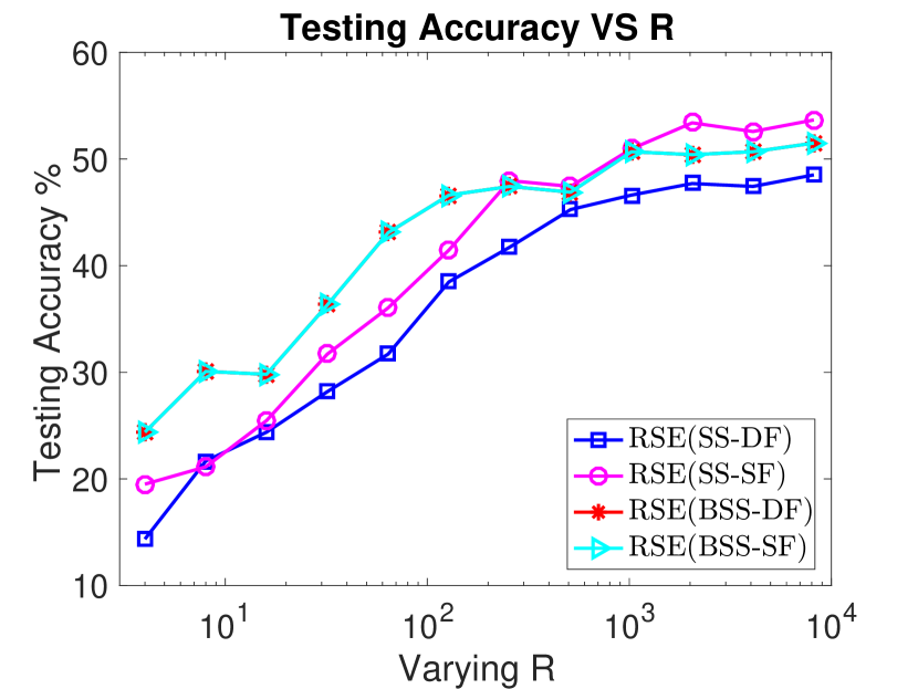
(a) ding-protein

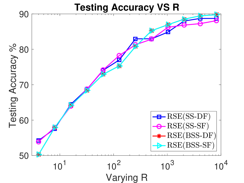
(b) splice

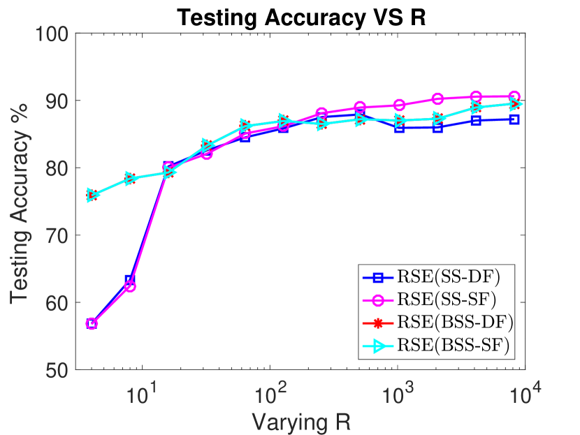
(c) dna3-class2

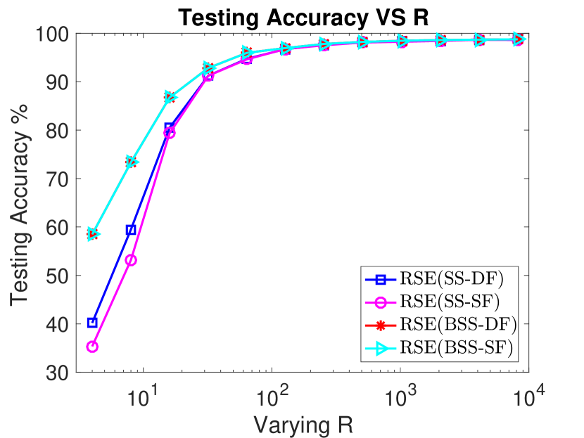
(d) mnist-str4

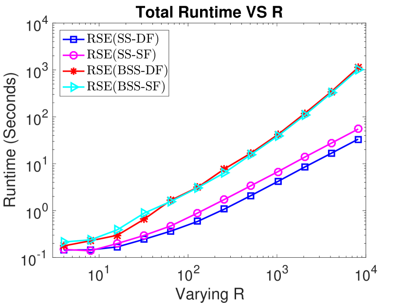
(e) ding-protein

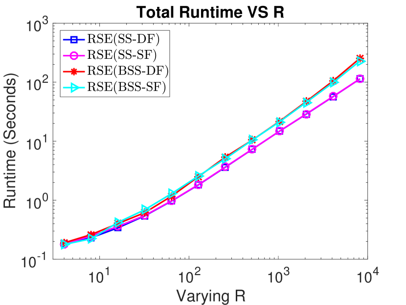
(f) splice

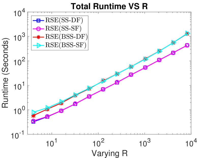
(g) dna3-class2

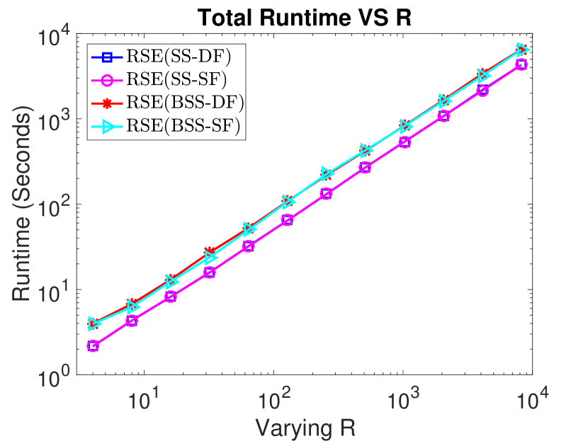
(h) mnist-str4

Figure 1. Test accuracy and computational runtime of RSE(SS-DF), RSE(SS-SF), RSE(BSS-DF), and RSE(BSS-SF) when varying $R$.

4.2. Comparison of RSE Against All Baselines

Setup. We assess the performance of RSE against five other state-of-the-art kernel and deep learning approaches in terms of both string classification accuracy and computational time. For RSE, we choose the variant RSE(BSS_SF) owing to its consistently robust performance and report the results on each dataset from Table 2. For SSK and ASK, we use the public available implementations of these two methods written in C and in Java, respectively. To achieve the best performance of SSK and ASK, following (Farhan et al., 2017; Kuksa et al., 2009) we generate the different combinations of ($k,m$)-mismatch kernel, where $k$ is between 8 and 12 and $m$ is between 2 and 5. We use LIBSVM (Chang and Lin, 2011) for these precomputed kernel matrices and search for the best hyperparameter (regularization) of SVM in the range of [1e-5 1e5]. For LSTM and GRU, all experiments were conducted on a server with 8 CPU cores and NVIDIA Tesla K80 accelerator with two GK210 GPU. However, to facilitate a relatively fair runtime comparison, we directly run two deep learning models on CPU only and report their runtime.

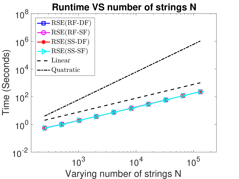
(a) Number of Strings $N$

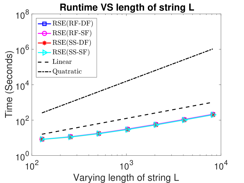
(b) Length of String $L$

Figure 2. Runtime for computing RSE string embeddings, and the overall runtime when varying number of strings $N$ and length of string $L$. (Default values: number of strings $N=10000$, length of string $L=512$). Linear and quadratic complexity are also plotted for easy comparisons.

Results. As shown in Table 3, RSE can consistently outperform or match all other baselines in terms of classification accuracy while requiring less computation time for achieving the same accuracy. The first interesting observation is that our method performs substantially better than SSK and ASK, often by a large margin, i.e., RSE achieves 25% - 33% higher accuracy than SSK and ASK on three protein datasets. This is because $(k,m)$-mismatch string kernel is sensitive to the strings of long length, which often causes the feature space size of the short sub-strings (k-mers) exponentially grow and leads to diagonal dominance problem. More importantly, using only small sub-strings extracted from the original strings results in an inherently local perspective and fails to capture the global properties of strings of long length. Secondly, in order to achieving the same accuracy, the required runtime of RSE could be significantly less than that of SSK and ASK. For instance, on dataset superfamily, RSE achieves the accuracy 46.56% using 3.7 second while SSK and ASK achieve similar accuracy 44.63% and 44.79% using 140.0 and 257.0 seconds respectively. Thirdly, RSE achieves much better performance than KSVM on all of datasets, highlighting the importance of truly p.d. kernel compared to the indefinite kernel even in the Krein space. Finally, compared to two state-of-the-art deep learning models, RSE still has shown clear advantages over LSTM and GRU, especially for the strings of long length. RSE achieves better accuracy than LSTM and GRU on 7 out of the total 9 datasets except on dna3-class3 and mnist-str8. It is well-known that Deep Learning based approaches typically require large amount of tranning data, which could be one of the important reasons why they performed worse on relatively small data but slightly better or similar performance on large data such as dna3-class3 and mnist-str8.

4.3. Accuracy and Runtime of RSE When Varying R

Setup. We now conduct experiments to investigate the behavior of four best variants of RSE by varying the number R of random strings. The hyperparameter $D_{max}$ is obtained from the previous cross-validations on the training set. We set $R$ in the range [4, 8192]. We report both testing accuracy and runtime when increasing random string embedding size $R$.

Results. Fig. 1 shows how the testing accuracy and runtime changes when increasing R. We can see that all selected variants of RSE converge very fast when increasing R from a small number (R = 4) to relatively large number. Interestingly, using block sub-strings (BSS) sampling strategy typically leads to a better convergence at the beginning since BSS could produce multiple random strings at every sampling time that sometimes offers much help in boosting the performance. However, when increasing $R$ to larger number, all variants converge similarly to the optimal performance of the exact kernel. This confirms our analysis in Theory 1 that the RGE approximation can guarantee the fast convergence to the exact kernel. Another important observation is that all variants of RSE scales linearly with increase in the size of the random string embedding $R$. This is a particularly important property for scaling up large-scale string kernels. On the other hand, one can easily achieve the good trade-off between the desired testing accuracy and the limited computational time, depending on the actual demands of the underlying applications.

4.4. Scalability of RSE When Varying Numbers of Strings $N$ and Length of String $L$

Setup. Next, we evaluate the scalability of RSE when varying number of strings $N$ and the length of a string $L$ on randomly generated string dataset. We change the number of strings in the range of $N=[128,\ 131072]$ and the length of a string in the range of $L=[128,\ 8192]$, respectively. When generating random string dataset, we choose its alphabet same as protein strings. We also set $D_{max}=10$ and $R=256$ for the hyperparameters related to RSE. We report the runtime for computing string embeddings using four variants of our method RSE.

Results. As shown in Fig. 2, we have two important observations about the scalability of RSE. First, Fig. 2(a) clearly shows RSE scales linearly when increasing the number of strings $N$. Second, Fig. 2(b) empirically corroborated that RSE also achieves linear scalability in terms of the length of string $L$. These emperical results provide a strong evidence to demonstrate that RSE derived from our newly proposed global string kernel indeed scales linearly in both number of string samples and length of string. Our method opens the door for developing a new family of string kernels that enjoy both higher accuracy and linear scalability on real-world string data.

5. Conclusions

In this paper, we present a new family of positive-definite string kernels that take into account the global properties hidden in the data strings through the global alignments measured by Edit Distance. Our Random String Embedding, derived from the proposed kernel through Random Feature approximation, enjoys double benefits of producing higher classification accuracy and scaling linearly in terms of both number of strings and the length of a string. Our newly defined global string kernels pave a simple yet effective way to handle real-world large-scale string data.

Several interesting future directions are listed below: i) our method can be further exploited with other distance measure that consider the global or local alignments; ii) other non-linear solver can be applied to potentially improve the classification of our embedding compared to our currently used linear SVM solver; iii) our method can be applied in the application domain like computational biology for the domain-specific problems.

References

- (1)
- Chang and Lin (2011) Chih-Chung Chang and Chih-Jen Lin. 2011. LIBSVM: a library for support vector machines. ACM transactions on intelligent systems and technology 2, 3 (2011), 27.
- Chen et al. (2016) Jie Chen, Lingfei Wu, Kartik Audhkhasi, Brian Kingsbury, and Bhuvana Ramabhadrari. 2016. Efficient one-vs-one kernel ridge regression for speech recognition. In ICASSP. IEEE, 2454–2458.
- Chen et al. (2009) Yihua Chen, Eric K Garcia, Maya R Gupta, Ali Rahimi, and Luca Cazzanti. 2009. Similarity-based classification: Concepts and algorithms. Journal of Machine Learning Research 10, Mar (2009), 747–776.
- Cho et al. (2014) Kyunghyun Cho, Bart Van Merriënboer, Dzmitry Bahdanau, and Yoshua Bengio. 2014. On the properties of neural machine translation: Encoder-decoder approaches. arXiv:1409.1259 (2014).
- Chung et al. (2014) Junyoung Chung, Caglar Gulcehre, KyungHyun Cho, and Yoshua Bengio. 2014. Empirical evaluation of gated recurrent neural networks on sequence modeling. arXiv:1412.3555 (2014).
- Cortes et al. (2004) Corinna Cortes, Patrick Haffner, and Mehryar Mohri. 2004. Rational kernels: Theory and algorithms. Journal of Machine Learning Research 5, Aug (2004), 1035–1062.
- Cristianini et al. (2000) Nello Cristianini, John Shawe-Taylor, et al. 2000. An introduction to support vector machines and other kernel-based learning methods. Cambridge university press.
- Fan et al. (2008) Rong-En Fan, Kai-Wei Chang, Cho-Jui Hsieh, Xiang-Rui Wang, and Chih-Jen Lin. 2008. LIBLINEAR: A library for large linear classification. Journal of machine learning research 9, Aug (2008), 1871–1874.
- Farhan et al. (2017) Muhammad Farhan, Juvaria Tariq, Arif Zaman, Mudassir Shabbir, and Imdad Ullah Khan. 2017. Efficient Approximation Algorithms for Strings Kernel Based Sequence Classification. In NIPS. 6938–6948.
- Frank and Asuncion (2010) Andrew Frank and Arthur Asuncion. 2010. UCI Machine Learning Repository [http://archive. ics. uci. edu/ml]. Irvine, CA: University of California. School of information and computer science 213 (2010).
- Gordon et al. (2003) Leo Gordon, Alexey Ya Chervonenkis, Alex J Gammerman, Ilham A Shahmuradov, and Victor V Solovyev. 2003. Sequence alignment kernel for recognition of promoter regions. Bioinformatics 19, 15 (2003), 1964–1971.
- Greene and Cunningham (2006) Derek Greene and Pádraig Cunningham. 2006. Practical solutions to the problem of diagonal dominance in kernel document clustering. In ICML. ACM, 377–384.
- Greff et al. (2017) Klaus Greff, Rupesh K Srivastava, Jan Koutník, Bas R Steunebrink, and Jürgen Schmidhuber. 2017. LSTM: A search space odyssey. IEEE transactions on neural networks and learning systems 28, 10 (2017), 2222–2232.
- Haasdonk and Bahlmann (2004) Bernard Haasdonk and Claus Bahlmann. 2004. Learning with distance substitution kernels. In Joint Pattern Recognition Symposium. Springer, 220–227.
- Haussler (1999) David Haussler. 1999. Convolution kernels on discrete structures. Technical Report. Department of Computer Science, University of California at Santa Cruz.
- Huang et al. (2014) Po-Sen Huang, Haim Avron, Tara N Sainath, Vikas Sindhwani, and Bhuvana Ramabhadran. 2014. Kernel methods match Deep Neural Networks on TIMIT.. In ICASSP. 205–209.
- Ionescu et al. (2017) Catalin Ionescu, Alin Popa, and Cristian Sminchisescu. 2017. Large-scale data-dependent kernel approximation. In AIStats. 19–27.
- Kingma and Ba (2014) Diederik P. Kingma and Jimmy Ba. 2014. Adam: A Method for Stochastic Optimization. CoRR abs/1412.6980 (2014).
- Kuang et al. (2005) Rui Kuang, Eugene Ie, Ke Wang, Kai Wang, Mahira Siddiqi, Yoav Freund, and Christina Leslie. 2005. Profile-based string kernels for remote homology detection and motif extraction. Journal of bioinformatics and computational biology 3, 03 (2005), 527–550.
- Kuksa et al. (2009) Pavel P Kuksa, Pai-Hsi Huang, and Vladimir Pavlovic. 2009. Scalable algorithms for string kernels with inexact matching. In NIPS. 881–888.
- Leslie et al. (2001) Christina Leslie, Eleazar Eskin, and William Stafford Noble. 2001. The spectrum kernel: A string kernel for SVM protein classification. In Biocomputing 2002. World Scientific, 564–575.
- Leslie et al. (2003) Christina Leslie, Eleazar Eskin, Jason Weston, and William Stafford Noble. 2003. Mismatch string kernels for SVM protein classification. In NIPS. Neural information processing systems foundation.
- Leslie and Kuang (2004) Christina Leslie and Rui Kuang. 2004. Fast string kernels using inexact matching for protein sequences. Journal of Machine Learning Research 5, Nov (2004), 1435–1455.
- Leslie et al. (2004) Christina S Leslie, Eleazar Eskin, Adiel Cohen, Jason Weston, and William Stafford Noble. 2004. Mismatch string kernels for discriminative protein classification. Bioinformatics 20, 4 (2004), 467–476.
- Levenshtein (1966) Vladimir I Levenshtein. 1966. Binary codes capable of correcting deletions, insertions, and reversals. In Soviet physics doklady, Vol. 10. 707–710.
- Lodhi et al. (2002) Huma Lodhi, Craig Saunders, John Shawe-Taylor, Nello Cristianini, and Chris Watkins. 2002. Text classification using string kernels. Journal of Machine Learning Research 2, Feb (2002), 419–444.
- Loosli et al. (2016) Gaëlle Loosli, Stéphane Canu, and Cheng Soon Ong. 2016. Learning SVM in Krein spaces. IEEE transactions on pattern analysis and machine intelligence 38, 6 (2016), 1204–1216.
- Needleman and Wunsch (1970) Saul B Needleman and Christian D Wunsch. 1970. A general method applicable to the search for similarities in the amino acid sequence of two proteins. Journal of molecular biology 48, 3 (1970), 443–453.
- Neuhaus and Bunke (2006) Michel Neuhaus and Horst Bunke. 2006. Edit distance-based kernel functions for structural pattern classification. Pattern Recognition 39, 10 (2006), 1852–1863.
- Rahimi and Recht (2008) Ali Rahimi and Benjamin Recht. 2008. Random features for large-scale kernel machines. In NIPS. 1177–1184.
- Rudi and Rosasco (2017) Alessandro Rudi and Lorenzo Rosasco. 2017. Generalization properties of learning with random features. In NIPS. 3218–3228.
- Saigo et al. (2004) Hiroto Saigo, Jean-Philippe Vert, Nobuhisa Ueda, and Tatsuya Akutsu. 2004. Protein homology detection using string alignment kernels. Bioinformatics 20, 11 (2004), 1682–1689.
- Schölkopf et al. (2004) Bernhard Schölkopf, Koji Tsuda, Jean-Philippe Vert, Director Sorin Istrail, Pavel A Pevzner, Michael S Waterman, et al. 2004. Kernel methods in computational biology. MIT press.
- Si et al. (2017) Si Si, Cho-Jui Hsieh, and Inderjit S Dhillon. 2017. Memory efficient kernel approximation. The Journal of Machine Learning Research 18, 1 (2017), 682–713.
- Smith and Waterman (1981) Temple F Smith and Michael S Waterman. 1981. Comparison of biosequences. Advances in applied mathematics 2, 4 (1981), 482–489.
- Smola and Vishwanathan (2003) Alex J Smola and SVN Vishwanathan. 2003. Fast kernels for string and tree matching. In NIPS. 585–592.
- Srivastava et al. (2014) Nitish Srivastava, Geoffrey E. Hinton, Alex Krizhevsky, Ilya Sutskever, and Ruslan Salakhutdinov. 2014. Dropout: a simple way to prevent neural networks from overfitting. Journal of Machine Learning Research 15, 1 (2014), 1929–1958.
- Waterman et al. (1991) MICHAEL S Waterman, JANA Joyce, and Mark Eggert. 1991. Computer alignment of sequences. Phylogenetic analysis of DNA sequences (1991), 59–72.
- Watkins (1999) Chris Watkins. 1999. Dynamic alignment kernels. NIPS (1999), 39–50.
- Weston et al. (2003) Jason Weston, Bernhard Schölkopf, Eleazar Eskin, Christina Leslie, and William Stafford Noble. 2003. Dealing with large diagonals in kernel matrices. Annals of the Institute of Statistical Mathematics 55, 2 (2003), 391–408.
- Williams and Seeger (2001) Christopher KI Williams and Matthias Seeger. 2001. Using the Nyström method to speed up kernel machines. In NIPS. 682–688.
- Wu et al. (2018a) Lingfei Wu, Pin-Yu Chen, Ian En-Hsu Yen, Fangli Xu, Yinglong Xia, and Charu Aggarwal. 2018a. Scalable spectral clustering using random binning features. In KDD. ACM, 2506–2515.
- Wu et al. (2016) Lingfei Wu, Ian EH Yen, Jie Chen, and Rui Yan. 2016. Revisiting random binning features: Fast convergence and strong parallelizability. In KDD. ACM, 1265–1274.
- Wu et al. (2018c) Lingfei Wu, Ian EH Yen, Kun Xu, Fangli Xu, Avinash Balakrishnan, Pin-Yu Chen, Pradeep Ravikumar, and Michael J Witbrock. 2018c. Word Mover’s Embedding: From Word2Vec to Document Embedding. EMNLP (2018), 4524–4534.
- Wu et al. (2018b) Lingfei Wu, Ian En-Hsu Yen, Fangli Xu, Pradeep Ravikuma, and Michael Witbrock. 2018b. D2KE: From Distance to Kernel and Embedding. arXiv:1802.04956 (2018).
- Wu et al. (2018d) Lingfei Wu, Ian En-Hsu Yen, Jinfeng Yi, Fangli Xu, Qi Lei, and Michael Witbrock. 2018d. Random Warping Series: A Random Features Method for Time-Series Embedding. In AIStats. 793–802.
- Xing et al. (2010) Zhengzheng Xing, Jian Pei, and Eamonn Keogh. 2010. A brief survey on sequence classification. ACM Sigkdd Explorations Newsletter 12, 1 (2010), 40–48.
- Yujian and Bo (2007) Li Yujian and Liu Bo. 2007. A normalized Levenshtein distance metric. IEEE transactions on pattern analysis and machine intelligence 29, 6 (2007), 1091–1095.