Instability of the big bang coordinate singularity
in a Milne-like universe

Abstract

We present a simplified dynamic-vacuum-energy model for a time-symmetric Milne-like universe. The big bang singularity in this simplified model, like the one in a previous model, is just a coordinate singularity with finite curvature and energy density. We then calculate the dynamic behavior of scalar metric perturbations and find that these perturbations destabilize the big bang singularity.

I Introduction

We have recently discussed two ways to “tame” the big bang singularity of the Friedmann solution Friedmann1922-1924 ; Weinberg1972 ; MisnerThorneWheeler2017 . The first way Klinkhamer2019 ; KlinkhamerWang2019-PRD ; KlinkhamerWang2019-LHEP ; Klinkhamer2019-revisited ; KlinkhamerWang2019-nonsing-bounce-pert is to consider a particular degenerate metric, which describes a spacetime defect with a characteristic length scale $b$ (the characteristic time scale is then $b/c$, where $c$ is the velocity of light in vacuum). The cosmic scale factor $a(t)$ remains finite at $t=t_{\text{bb}}\equiv 0$ and the singular big bang is turned into a nonsingular bounce.

The second way Ling2018 ; KlinkhamerLing2019 keeps a smooth spacetime (with the spatially-hyperbolic Robertson–Walker metric) but allows only vacuum energy to be present. There is still the big bang at $t=t_{\text{bb}}\equiv 0$ with vanishing cosmic scale factor, $a(0)=0$, but there is now only a coordinate singularity with finite values of the curvature scalars. The behavior at $t=0$ resembles that of the so-called Milne universe Milne1932 (cf. Sec. 5.3 of Ref. BirrellDavies1982 and Sec. 1.3.5 of Ref. Mukhanov2005 ), which corresponds to Minkowski spacetime in expanding/contracting coordinates. More precisely, the spacetime of Refs. Ling2018 ; KlinkhamerLing2019 is called a “Milne-like universe,” as it corresponds, at $t=0$, to a slice of de Sitter spacetime rather than Minkowski spacetime.

The physics model of Ref. KlinkhamerLing2019 relies on the $q$-theory approach to the cosmological constant problem KlinkhamerVolovik2008a ; KlinkhamerVolovik2008b ; KlinkhamerVolovik2009 ; KlinkhamerVolovik2016 and shows that the positive vacuum energy at $t=0$ reduces to zero as the model universe evolves, $|t|\to\infty$. But the explicit $q$-theory for the Milne-like model of Ref. KlinkhamerLing2019 is rather complicated.

The goal of the present article is, first, to simplify the $q$-theory Milne-like model and, second, to study perturbations near $t=0$. This last topic is relevant to issues such as stability and cross-big-bang information transfer. Precisely these issues have already been discussed in Ref. KlinkhamerWang2019-nonsing-bounce-pert for the case of the degenerate-metric nonsingular bounce, but the case of the Milne-like model is more subtle.

II Simplified model for a Milne-like universe

II.1 Action and field equations

The $q$-theory model of a Milne-like universe in Ref. KlinkhamerLing2019 uses a postulated dissipative term in the dynamic equation for the $q$-field. A relatively simple alternative is to use an action with explicit derivative terms of the $q$-field KV2016-q-ball ; KV2016-q-DM ; KV2016-more-on-q-DM ; KlinkhamerMistele2017 ; Klinkhamer-etal2019 . Specifically, we take the following action KlinkhamerVolovik2008a ; KV2016-q-DM :

$$S = -\int\,d^{4}x\,\sqrt{-g}\,\left(\frac{R}{16\pi G_{N}}+\epsilon(q)\right.\left.+\frac{1}{2}\,(q_{0})^{-1}\,g^{\alpha\beta}\,(\nabla_{\alpha}\,q)\,(\nabla_{\beta}\,q)\right),$$ (1a)

$$\epsilon(q) = \sigma(q)+\Lambda\,,\quad\frac{d\sigma(q)}{dq}\neq 0\,,$$ (1b)

$$F_{\alpha\beta\gamma\delta} \equiv \nabla_{[\alpha}A_{\beta\gamma\delta]}\,,\quad F_{\alpha\beta\gamma\delta}=q\,\sqrt{-g}\,\epsilon_{\alpha\beta\gamma\delta}\,,$$ (1c)

where $A$ is a three-form gauge field with corresponding four-form field strength $F\propto q$, so that the $q$-field has mass dimension $2$. In (1b), $\Lambda$ is an initial cosmological constant and $\sigma(q)$ a generic even function of $q$. The conventions for the curvature tensors follow those of Ref. Weinberg1972 .

Let us now give a brief review of the resulting field equations. First, there is the following nonlinear Klein–Gordon equation KV2016-q-DM :

$$(q_{0})^{-1}\,\Box\,q=\frac{d\rho_{V}(q)}{dq}\,,$$ (2)

in terms of the vacuum energy density $\rho_{V}(q)$ defined by

$$\rho_{V}(q)\equiv\epsilon(q)-\mu_{0}\,q\,,$$ (3)

where the constant $\mu_{0}$ traces back to the solution of the generalized Maxwell equation (the constant $\mu_{0}$ can be interpreted as a chemical potential KlinkhamerVolovik2008a ; KlinkhamerVolovik2008b ). Second, there is the Einstein equation KV2016-q-DM ,

$$R_{\alpha\beta}-\frac{1}{2}\,g_{\alpha\beta}\,R=-8\pi G_{N}\,T_{\alpha\beta}^{\,\text{(q-vac)}}\,,$$ (4a)

$$T_{\alpha\beta}^{\,\text{(q-vac)}}=-\left(\rho_{V}(q)+\frac{1}{2}\,(q_{0})^{-1}\,\nabla_{\gamma}\,q\,\nabla^{\gamma}q\right)\,g_{\alpha\beta}+(q_{0})^{-1}\,\nabla_{\alpha}\,q\,\nabla_{\beta}\,q\,.$$ (4b)

The energy-momentum-tensor (4b) describes the gravitational effects of the quantum vacuum, which is here characterized by the $q$-field.

For the simplified theory (1), we have that the energy momentum tensor (4b) of the composite pseudoscalar field $q(x)$ has the same structure as the one of a fundamental (pseudo-)scalar field $\phi(x)$. This implies that previous results for a gravitating fundamental scalar field $\phi(x)$ carry over, as long as $\mu_{0}$ has the appropriate dependence on $\Lambda$ (see, e.g., the discussion of the penultimate paragraph in Sec. 2 of Ref.  Klinkhamer-etal2019 ).

II.2 Ansätze

The metric Ansatz is given by the spatially-hyperbolic ($k=-1$) Robertson–Walker metric MisnerThorneWheeler2017 in terms of comoving spatial coordinates $\{\chi,\,\vartheta,\,\varphi\}$,

$$ds^{2} \equiv g_{\mu\nu}(x)\,dx^{\mu}\,dx^{\nu}=-dt^{2}+a^{\,2}(t)\,\left[d\chi^{2}+\sinh^{2}(\chi)\,\Big{(}d\vartheta^{2}+\sin^{2}(\vartheta)\,d\varphi^{2}\Big{)}\right]\,,$$ (5a)

$$t \in (-\infty,\,\infty)\,,\quad\chi\in[0,\,\infty)\,,\quad\vartheta\in[0,\,\pi]\,,\quad\varphi\in[0,\,2\pi)\,,$$ (5b)

where the infinite range of the cosmic time coordinate $t$ is to be noted.

We will use the Ricci curvature scalar $R(x)\equiv g^{\nu\sigma}(x)\,g^{\mu\rho}(x)\,R_{\mu\nu\rho\sigma}(x)$ and the Kretschmann curvature scalar $K(x)\equiv R^{\mu\nu\rho\sigma}(x)\,R_{\mu\nu\rho\sigma}(x)$ as diagnostic tools for the behavior near the big bang with $a(0)=0$. From the metric (5), these curvature scalars are

$$R[a(t)] = 6\,\left[\frac{\ddot{a}(t)}{a(t)}+\left(\frac{\dot{a}(t)}{a(t)}\right)^{2}-\frac{1}{a^{2}(t)}\right]\,,$$ (6a)

$$K[a(t)] = 12\,\left[\left(\frac{\ddot{a}(t)}{a(t)}\right)^{2}+\left(\left(\frac{\dot{a}(t)}{a(t)}\right)^{2}-\frac{1}{a^{2}(t)}\right)^{2}\right]\,,$$ (6b)

where the overdot stands for differentiation with respect to $t$.

The homogenous $q$-field Ansatz is given by

$$q=q(t)\,.$$ (7)

Following-up on the remark below (4b), we observe that the homogeneous $q$-field has an energy momentum tensor equal to the one of a perfect fluid with the following energy density and pressure:

$$\rho_{\text{q-vac}} = \frac{1}{2}\,(q_{0})^{-1}\,\left(\frac{dq}{dt}\right)^{2}+\rho_{V}(q)\,,$$ (8a)

$$P_{\text{q-vac}} = \frac{1}{2}\,(q_{0})^{-1}\,\left(\frac{dq}{dt}\right)^{2}-\rho_{V}(q)\,,$$ (8b)

for the $q$ function from (7). Observe that the Lorentz-invariant behavior $P_{\text{q-vac}}=-\rho_{\text{q-vac}}$ only holds for a constant $q$-field KlinkhamerVolovik2008a .

II.3 ODEs

We now introduce dimensionless variables ($\hbar=c=8\pi G_{N}=1$). Writing $\tau$ for the dimensionless version of the cosmic time coordinate $t$, we have that $f(\tau)$ is the dimensionless variable corresponding to $q(t)$, $r_{V}(\tau)$ the dimensionless variable corresponding to $\rho_{V}(t)$, and $p_{V}(\tau)$ the dimensionless variable corresponding to $P_{V}(t)$. In addition, $u_{0}$ is the dimensionless constant (chemical potential) corresponding to $\mu_{0}$ and $\lambda$ the dimensionless cosmological constant corresponding to $\Lambda$.

The ordinary differential equations (ODEs) for $a(\tau)$ and $f(\tau)$ are the dimensionless second- and first-order Friedmann equations and the dimensionless nonlinear Klein–Gordon equation:

$$\frac{\ddot{a}}{a}=-\frac{1}{3}\,\Big{(}\dot{f}^{2}-r_{V}\Big{)}\,,$$ (9a)

$$\left(\frac{\dot{a}}{a}\right)^{2}-\frac{1}{a^{2}}=\frac{1}{3}\,\left(\frac{1}{2}\,\dot{f}^{2}+r_{V}\right)\,,$$ (9b)

$$\ddot{f}+3\,\left(\frac{\dot{a}}{a}\right)\,\dot{f}=-\frac{d}{df}\,r_{V}\,,$$ (9c)

$$r_{V}(f)=\epsilon(f)-u_{0}\,f\,,$$ (9d)

where the overdot now stands for differentiation with respect to $\tau$. Observe the invariance of these ODEs under the following time-reversal transformation:

$$\tau \to -\tau\,,$$ (10a)

$$a(\tau) \to -a(-\tau)\,,$$ (10b)

$$f(\tau) \to f(-\tau)\,,$$ (10c)

with the characteristic odd behavior of the scale factor $a(\tau)$ for the Milne-like universe. The boundary conditions at $\tau=0$ are taken as follows:

$$a(0) = 0\,,$$ (11a)

$$f(0) = f_{\text{bb}}\,,\;\;\text{with}\;\;r_{V}(f_{\text{bb}})>0\,,$$ (11b)

$$\dot{f}(0) = 0\,.$$ (11c)

The model ODEs (9) with boundary conditions (11) constitute the main result of Sec. II.

For the numerical calculations later on, we use the following explicit energy-density function KlinkhamerVolovik2016 :

$$\epsilon(f) = \lambda+f^{2}+1/f^{2}\,.$$ (12)

From the equilibrium condition

$$\epsilon(f)-f\,\frac{d\epsilon(f)}{df} = 0\,,$$ (13)

we get, with the particular function (12), the following equilibrium value $f_{0}$ (real and positive) and corresponding chemical potential $u_{0}$ :

$$f_{0} = \sqrt{\Big{(}\lambda+\sqrt{12+\lambda^{2}}\,\Big{)}\Big{/}2}\,,$$ (14a)

$$u_{0} = \left.\frac{d\epsilon(f)}{df}\right|_{f=f_{0}}=\frac{2\,{\sqrt{2}}\,\left(4+{\lambda}^{2}+\lambda\,{\sqrt{12+{\lambda}^{2}}\,}\right)}{{\left(\lambda+{\sqrt{12+{\lambda}^{2}}}\right)}^{3/2}}\,.$$ (14b)

With the explicit result (14b) for $u_{0}$, we then obtain the dimensionless energy density (9d), which enters the ODEs (9a), (9b), and (9c). It can be verified that the following equilibrium properties hold:

$$r_{V}(f_{0}) = 0\,,$$ (15a)

$$dr_{V}/df\big{|}_{f=f_{0}} = 0\,,$$ (15b)

in addition to having a positive second derivative corresponding to a positive inverse vacuum compressibility KlinkhamerVolovik2008a .

For completeness, we also give the dimensionless versions of the quantum-vacuum energy density and pressure from (8), and introduce the corresponding equation-of-state parameter $w$ :

$$r_{\text{q-vac}} = \frac{1}{2}\,\dot{f}^{2}+r_{V}(f)\,,$$ (16a)

$$p_{\text{q-vac}} = \frac{1}{2}\,\dot{f}^{2}-r_{V}(f)\,,$$ (16b)

$$w_{\text{q-vac}} \equiv p_{\text{q-vac}}/r_{\text{q-vac}}\,,$$ (16c)

with $f=f(\tau)$.

II.4 Analytic results

For an appropriate fixed value of $f(\tau)$, the two Friedmann ODEs (9a) and (9b) with boundary conditions (11) are solved by the following functions:

$$\widetilde{a}(\tau) = \frac{1}{\sqrt{r_{V}(f_{\text{bb}})/3}}\;\sinh\left(\sqrt{r_{V}(f_{\text{bb}})/3}\;\tau\right)\,,$$ (17a)

$$\widetilde{f}(\tau) = f_{\text{bb}}\,,$$ (17b)

with $r_{V}(f_{\text{bb}})>0$. However, the functions (17) do not solve the nonlinear Klein–Gordon equation (9c), as its left-hand side vanishes trivially but not its right-hand side.

The combined solution of the ODEs (9) with boundary conditions (11) can be obtained by a perturbative series expansion,

$$a_{\text{pert}}(\tau) = \tau+c_{3}\,\tau^{3}+c_{5}\,\tau^{5}+c_{7}\,\tau^{7}+\ldots\,,$$ (18a)

$$f_{\text{pert}}(\tau) = f_{\text{bb}}\,+d_{2}\,\tau^{2}+d_{4}\,\tau^{4}+d_{6}\,\tau^{6}+\ldots\,.$$ (18b)

Defining

$$r_{0} \equiv r_{V}(f_{\text{bb}})>0\,,$$ (19a)

$$r_{n} \equiv \left.\frac{d^{n}r_{V}(f)}{(df)^{n}}\right|_{f=f_{\text{bb}}}\,,\;\;\text{for}\;\;n\geq 1\,,$$ (19b)

the ODEs then give the following results for the coefficients:

$$\overline{c}_{3} = \frac{r_{0}}{18}\,,$$ (20a)

$$\overline{c}_{5} = \frac{8\,r_{0}^{2}-27\,r_{1}^{2}}{8640}\,,$$ (20b)

$$\overline{c}_{7} = \frac{16\,r_{0}^{3}-54\,r_{0}\,r_{1}^{2}+405\,r_{1}^{2}\,r_{2}}{2177280}\,,$$ (20c)

$$\overline{d}_{2} = -\frac{r_{1}}{8}\,,$$ (21a)

$$\overline{d}_{4} = \frac{r_{1}\,\left(2\,r_{0}+3\,r_{2}\right)}{576}\,,$$ (21b)

$$\overline{d}_{6} = -\frac{r_{1}\,\left(112\,r_{0}^{2}+162\,r_{1}^{2}+180\,r_{0}\,r_{2}+90\,{r_{2}}^{2}+135\,r_{1}\,r_{3}\right)}{829440}\,.$$ (21c)

For the interpretation of (18a) and (18b) as perturbative series, it is appropriate to consider $r_{V}$ as the “small” perturbation, in line with the structure of the obtained coefficients (20) and (21).

With the perturbative solution (18b) and (21), we obtain the following series expansions of the dimensionless quantum-vacuum energy density $r_{\text{q-vac}}$ from (16a) and pressure $p_{\text{q-vac}}$ from (16b):

$$r_{\text{q-vac,\;pert}}(\tau) = r_{0}-\frac{3\,r_{1}^{2}}{32}\,{\tau}^{2}+\frac{r_{1}^{2}\,r_{2}}{128}\,{\tau}^{4}+\text{O}(\tau^{6})\,,$$ (22a)

$$p_{\text{q-vac,\;pert}}(\tau) = -r_{0}+\frac{5\,r_{1}^{2}}{32}\,{\tau}^{2}-\frac{r_{1}^{2}\,\left(8\,r_{0}+21\,r_{2}\right)}{1152}\,{\tau}^{4}+\text{O}(\tau^{6})\,,$$ (22b)

where the cosmological-constant behavior ($r_{\text{q-vac}}=-p_{\text{q-vac}}$) disappears as $\tau$ moves away from $\tau=0$.

With the perturbative solution (18a) and (20), we obtain the following series expansions of the dimensionless Ricci curvature scalar $R$ from (6a) and the dimensionless Kretschmann curvature scalar $K$ from (6b):

$$R_{\text{pert}}(\tau) = 4\,r_{0}-\frac{9\,r_{1}^{2}}{16}\,{\tau}^{2}+\frac{r_{1}^{2}\,\left(r_{0}+3\,r_{2}\right)}{48}\,{\tau}^{4}+\text{O}(\tau^{6})\,,$$ (23a)

$$K_{\text{pert}}(\tau) = \frac{8\,r_{0}^{2}}{3}-\frac{3\,r_{0}\,r_{1}^{2}}{4}\,{\tau}^{2}+\frac{r_{1}^{2}\,\left(64\,r_{0}^{2}+135\,r_{1}^{2}+192\,r_{0}\,r_{2}\right)}{2304}\,{\tau}^{4}+\text{O}(\tau^{6})\,,$$ (23b)

which illustrate the regular behavior at $\tau=0$ of the Milne-like universe.

Our focus in this article is on the behavior near the big bang at $\tau=0$, but we can also give the asymptotic solution for $|\tau|\to\infty$. With the near-equilibrium behavior $r_{V}(f)\propto\big{(}f-f_{0}\big{)}^{2}$, the ODEs (9) are solved by the following asymptotic solution:

$$a_{\text{asymp}}(\tau) \sim \tau\,,$$ (24a)

$$f_{\text{asymp}}(\tau) \sim f_{0}\,,$$ (24b)

which corresponds to the Milne universe Milne1932 ; BirrellDavies1982 ; Mukhanov2005 with a nongravitating quantum vacuum in equilibrium.

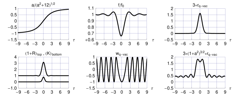
Figure 1: Numerical solution of the dimensionless ODEs (9) with energy-density function (12) for model parameter $\lambda=1$. The boundary conditions at $\tau=0$ are $\{a(0),\,f(0),\,\dot{f}(0)\}=\{0,\,1,\,0\}$, hence $f_{\text{bb}}=1$ in the notation of (11). The approximate analytic solution for $\tau\in[-\Delta\tau,\,\Delta\tau]$ is given by (17) and the numerical solution is obtained for $\tau\in[-\tau_{\text{max}},\,-\Delta\tau]\cup[\Delta\tau,\,\tau_{\text{max}}]$ with matching boundary conditions at $\tau=\pm\Delta\tau$, for $\Delta\tau=1/100$ and $\tau_{\text{max}}=2\times 10^{2}$. Shown, over a reduced time interval, are the dynamic variables $a(\tau)$ and $f(\tau)$, together with the corresponding dimensionless quantum-vacuum energy density $r_{\text{q-vac}}(\tau)$ from (16a), the equation-of-state parameter $w_{\text{q-vac}}(\tau)$ from (16c), the dimensionless Ricci curvature scalar $R(\tau)$ from (6a), and the dimensionless Kretschmann curvature scalar $K(\tau)$ from (6b). The bottom-left panel shows $(1+R)$ as the top curve and $K$ as the bottom curve. The bottom-right panel shows $r_{\text{q-vac}}$ multiplied by $3\,(1+a^{2})^{3/2}$. The dimensionless $q$-field energy density and pressure at $\tau=0$ take the following values: $r_{\text{q-vac}}(0)\approx 0.537358$ and $p_{\text{q-vac}}(0)=-r_{\text{q-vac}}(0)$. The dimensionless $q$-field has the Minkowski equilibrium value $f_{0}\approx 1.51749$ from (14a).

For later use, we give an approximate solution which interpolates between (18) at lowest order and (24):

$$a_{\text{approx}}(\tau) = \tau\,,$$ (25a)

$$f_{\text{approx}}(\tau) = \frac{f_{\text{bb}}+f_{0}\,(\tau/\tau_{\text{mid}})^{2}}{1+(\tau/\tau_{\text{mid}})^{2}}\,,$$ (25b)

where the optimal value of $\tau_{\text{mid}}$ needs to be determined but we will just set $\tau_{\text{mid}}=1$.

II.5 Numerical results

Figure 1 shows numerical results for the case of $\lambda=1$ and $f_{\text{bb}}=1$. As regards the cosmic scale factor $a(\tau)$, these results are similar to those of Ref. KlinkhamerLing2019 , which employed a source term to transfer energy from the vacuum sector to the matter sector. Here, we only have the quantum vacuum, but temporal fluctuations of the $q$-field now carry energy which can be red-shifted. From the results of Fig. 1, we see that the onset of the temporal oscillations occurs at $|\tau|\sim 2$ and that the energy density drops asymptotically as $r_{\text{q-vac}}\propto 1/(a^{2})^{3/2}$. Later, we will also consider spatial fluctuations of the $q$-field, whose energy can, in principle, be transported away to infinity.

III Scalar metric perturbations

III.1 Background fields

The unperturbed spatially-hyperbolic Robertson–Walker (RW) metric can be rewritten as follows MisnerThorneWheeler2017 ; Mukhanov-etal1992 :

$${ds^{2}}\Big{|}_{\text{RW}}=\Omega^{2}(\eta)\left[-d{\eta}^{2}+\frac{dx^{2}+dy^{2}+dz^{2}}{\big{(}1-\big{[}x^{2}+y^{2}+z^{2}\big{]}\big{/}4\big{)}^{2}}\right]\,,$$ (26)

where we have used the conformal time coordinate $\eta$ given by

$$\Omega(\eta),d\eta\equiv dt\,.$$ (27)

Remark that all coordinates $\eta\,,x\,,y$ and $z$ are dimensionless in the metric (26), but that $\Omega(\eta)$ and the corresponding scale factor $a(t)$ have the dimensions of a length. For more discussion about this spatially-hyperbolic metric, see, e.g., the text below Eqs. (27.25b) and (27.26) in Ref. MisnerThorneWheeler2017 .

For the dynamic $q$-field, the homogeneous Ansatz is simply

$$q(\eta\,,\mathbf{x})=\overline{q}(\eta)\,,$$ (28)

where $\overline{q}(\eta)$ is assumed to be nonzero and positive [the behavior of $\overline{q}(t)$ is shown in the top-mid panel of Fig. 1]. Henceforth, a bar over a quantity denotes its unperturbed (background) value. Logically, $\Omega(\eta)$ or $a(t)$ would also require a bar, but we refrain from doing so, for the sake of legibility.

The energy-momentum tensor from the background $q$-field is

$$\overline{T}^{0}_{\;0} = -\left[\frac{1}{2}\,\frac{(q_{0})^{-1}}{\Omega^{2}}\,(\overline{q}^{\,\prime})^{2}+\rho_{V}(\overline{q})\right]\,,$$ (29a)

$$\overline{T}^{i}_{\;j} = \left[\frac{1}{2}\,\frac{(q_{0})^{-1}}{\Omega^{2}}\,(\overline{q}^{\,\prime})^{2}-\rho_{V}(\overline{q})\right]\,\delta^{i}_{\;j}\,,$$ (29b)

$$\overline{T}^{0}_{\;j} = 0\,,$$ (29c)

where the prime stands for differentiation with respect to $\eta$ and the Latin indices $i$ and $j$ run over $\{1,\,2,\,3\}$.

III.2 Perturbed fields

In the conformal-Newtonian gauge, the perturbed spatially-hyperbolic RW metric is given by Mukhanov-etal1992

$$ds^{2}\Big{|}_{\text{RW-perturbed}}^{\text{(conformal-Newtonian-gauge)}}=$$

$$\Omega^{2}(\eta)\,\left[-(1+2\,\Phi)\,d{\eta}^{2}+\frac{1-2\,\Psi}{\big{(}1-\big{[}x^{2}+y^{2}+z^{2}\big{]}\big{/}4\big{)}^{2}}\;\big{(}dx^{2}+dy^{2}+dz^{2}\big{)}\right]\,,$$ (30)

where the metric perturbations $\Phi$ and $\Psi$ are functions of all spacetime coordinates $\{\eta,\,x,\,y,\,z\}$.

For scalar metric perturbations, the corresponding $q$-field can be decomposed into two parts,

$$q(\eta\,,\mathbf{x})=\overline{q}(\eta)+\delta q(\eta,\mathbf{x})\,,$$ (31)

where $\mathbf{x}$ are the spatial coordinates and $\delta q$ is a small perturbation satisfying $|\delta q|\ll\overline{q}$, for nonzero and positive $\overline{q}(\eta)$. By abuse of notation, we will also write

$$q(t\,,\mathbf{x})=\overline{q}(t)+\delta q(t,\mathbf{x})\,,$$ (32)

if, later, we use the original cosmic time coordinate $t$ from (5) and (27).

III.3 Perturbation equations of motion

For the perturbed metric (III.2) and the perturbed $q$-field (31), the first-order perturbation to the energy-momentum tensor (4b) is given by

$$\delta T^{0}_{\;0} = -\delta\rho_{V}+\frac{(q_{0})^{-1}}{\Omega^{2}}\,(\overline{q}^{\,\prime})^{2}\,\Phi-\frac{(q_{0})^{-1}}{\Omega^{2}}\overline{q}^{\,\prime}\delta q^{\,\prime}\,,$$ (33a)

$$\delta T^{i}_{\;j} = -\delta^{i}_{\;j}\left[\delta\rho_{V}+\frac{(q_{0})^{-1}}{\Omega^{2}}\,(\overline{q}^{\,\prime})^{2}\,\Phi-\frac{(q_{0})^{-1}}{\Omega^{2}}\overline{q}^{\,\prime}\delta q^{\,\prime}\right]\,,$$ (33b)

$$\delta T^{0}_{\;j} = -\frac{(q_{0})^{-1}}{\Omega^{2}}\overline{q}^{\,\prime}\,\partial_{j}\,\delta q\,.$$ (33c)

With (33), the perturbed Einstein tensor from the metric (III.2) gives the following equations of motion for the perturbed fields (cf. Ref. Mukhanov-etal1992 ):

$$-3\,\mathcal{H}\,\left(\mathcal{H}\,\Phi+\Phi^{\,\prime}\right)+\nabla^{2}\,\Phi-3\,\Phi=-4\pi G_{N}\left[-\Omega^{2}\,\delta\rho_{V}+(q_{0})^{-1}\,(\overline{q}^{\,\prime})^{2}\,\Phi-(q_{0})^{-1}\overline{q}^{\,\prime}\,\delta q^{\,\prime}\right],$$ (34a)

$$\left(2\,\mathcal{H}^{\,\prime}+\mathcal{H}^{2}\right)\,\Phi+\Phi^{\prime\prime}+3\,\mathcal{H}\,\Phi^{\prime}+\Phi=-4\pi G_{N}\left[\Omega^{2}\,\delta\rho_{V}+(q_{0})^{-1}\,(\overline{q}^{\,\prime})^{2}\,\Phi-(q_{0})^{-1}\overline{q}^{\,\prime}\,\delta q^{\,\prime}\right],$$ (34b)

$$\partial_{j}\left(\mathcal{H}\,\Phi+\Phi^{\prime}\right)=4\pi G_{N}\,(q_{0})^{-1}\,\overline{q}^{\,\prime}\,\partial_{j}\,\delta q\,,$$ (34c)

with the definition

$$\mathcal{H}\equiv\Omega^{\,\prime}/\Omega$$ (35)

and using

$$\Psi=\Phi\,,$$ (36)

as follows from the perturbed off-diagonal spatial Einstein equation.

Remark that $\nabla^{2}$ in (34a) is the Laplace–Beltrami operator on the three-dimensional constant-curvature hyperbolic space ($\mathbb{H}^{3}$). With our spatial $\{x\,,y,\,z\}$ coordinates, this operator reads explicitly

$$\nabla^{2}\Phi = \left(\frac{x^{2}+y^{2}+z^{2}}{4}-1\right)^{2}\,\left(\partial^{2}_{x}\,\Phi+\partial^{2}_{y}\,\Phi+\partial^{2}_{z}\,\Phi\right)$$ (37)

$$+\left(\frac{1}{2}-\frac{x^{2}+y^{2}+z^{2}}{8}\right)\,\left(x\,\partial_{x}\,\Phi+y\,\partial_{y}\,\Phi+z\,\partial_{z}\,\Phi\right)\,.$$

Remark also that, in three-dimensional hyperbolic space, we have the following eigenvalue equation for $\nabla^{2}$ :

$$\nabla^{2}\,Q_{k}(\mathbf{x})=-(k^{2}+1)\,Q_{k}(\mathbf{x})\,,$$ (38)

where $Q_{k}$ are the eigenfunctions (with further labels suppressed) and $-(k^{2}+1)$ the eigenvalues VilenkinSmorodinsky1964 ; KodamaSasaki1985 ; CornishSpergel1999 . In our later discussion, we will take the non-negative real number $k$ as the physical wavenumber of the $\Phi$ field.

From (34a) and (34b), we have the following partial differential equation (PDE):

$$\Phi^{\prime\prime}+6\,\mathcal{H}\,\Phi^{\prime}+2\,\left(\mathcal{H}^{\prime}+2\,\mathcal{H}^{2}+2\right)\,\Phi-\nabla^{2}\,\Phi=-8\pi G_{N}\,\Omega^{2}\,\delta\rho_{V}\,.$$ (39)

Notice that, with the conformal time coordinate $\eta$, the background nonlinear Klein–Gordon equation (2) is given by

$$\overline{q}^{\,\prime\prime}+2\,\mathcal{H}\,\overline{q}^{\,\prime}+q_{0}\,\Omega^{2}\,\frac{d\rho_{V}(q)}{dq}=0\,,$$ (40)

so that we have

$$\Omega^{2}\,\delta\rho_{V}=\Omega^{2}\,\frac{d\rho_{V}(q)}{dq}\,\delta q=-\frac{\overline{q}^{\,\prime\prime}+2\,\mathcal{H}\,\overline{q}^{\,\prime}}{\overline{q}^{\,\prime}}\;\frac{\mathcal{H}\,\Phi+\Phi^{\prime}}{4\pi G_{N}}\,,$$ (41)

where we have used (34c) to express $\delta q$ in terms of $\Phi$ and $\Phi^{\prime}$ ,

$$\delta q=(4\pi G_{N})^{-1}q_{0}\,\frac{\mathcal{H}\,\Phi+\Phi^{\prime}}{\overline{q}^{\,\prime}}\,.$$ (42)

With (41), the PDE (39) can be written as

$$\Phi^{\prime\prime}+\,2\left(\mathcal{H}-\frac{\overline{q}^{\,\prime\prime}}{\overline{q}^{\,\prime}}\right)\Phi^{\prime}+2\,\left(\mathcal{H}^{\prime}-\frac{\mathcal{H}\,\overline{q}^{\,\prime\prime}}{\overline{q}^{\,\prime}}+2\right)\,\Phi-\nabla^{2}\,\Phi=0\,,$$ (43)

which is the final equation of motion for the metric perturbation $\Phi(\eta,\,\mathbf{x})$.

Returning to the original cosmic time coordinate $t$ from (5a), we rewrite (43) as follows for $\Phi(t,\,\mathbf{x})$:

$$\ddot{\Phi}+\left(\frac{\dot{a}}{a}-\frac{2\,\ddot{\overline{q}}}{\dot{\overline{q}}}\right)\dot{\Phi}+2\left(\frac{\ddot{a}}{a}-\frac{\dot{a}^{2}}{a^{2}}-\frac{\dot{a}}{a}\,\frac{\ddot{\overline{q}}}{\dot{\overline{q}}}+\frac{2}{a^{2}}\right)\Phi-\frac{\nabla^{2}\,\Phi}{a^{2}}=0\,,$$ (44)

where the overdot stands for the partial derivative with respect to $t$. Writing the solution of (44) as $\widehat{\Phi}(t,\,\mathbf{x})$ and using (42), the $q$-field perturbation solution $\widehat{\delta q}(t,\,\mathbf{x})$ is given by

$$\widehat{\delta q}/q_{0}=2\,\frac{(E_{\text{planck}})^{2}}{q_{0}}\;\frac{H\,\widehat{\Phi}+\dot{\widehat{\Phi}}}{\dot{\overline{q}}/q_{0}}\,,$$ (45)

in terms of the reduced Planck energy

$$E_{\text{planck}}\equiv\sqrt{1/(8\pi\,G_{N})}\approx 2.44\times 10^{18}\,\text{GeV}\,.$$ (46)

Equations (44) and (45) constitute the main general result of Sec. III.

III.4 Perturbation solutions

From now on, we use the dimensionless variables introduced in the first paragraph of Sec. II.3 and consider only a spherical-wave scalar metric perturbation $\Phi$ and a spherical-wave perturbation $\delta f$ of the dimensionless $q$-field,

$$\Phi(\tau,\,\mathbf{x}) = \int_{0}^{\infty}dk\,\sum_{l,m}\;\Phi_{klm}(\tau)\;Q_{klm}(\chi,\,\theta,\,\phi)\,,$$ (47a)

$$\delta f(\tau,\,\mathbf{x}) = \int_{0}^{\infty}dk\,\sum_{l,m}\;\delta f_{klm}(\tau)\;Q_{klm}(\chi,\,\theta,\,\phi)\,,$$ (47b)

where $\{\chi,\,\theta,\,\phi\}$ are the dimensionless coordinates from (5) and $Q_{klm}(\chi,\,\theta,\,\phi)$ the eigenmodes of the hyperbolic Laplace operator CornishSpergel1999 . For the labels of the eigenmodes, we prefer to use the wavenumber $k$ with range

$$k\in[0,\,\infty)\,,$$ (48)

as we already have used the symbol $q$ for the physical $q$-field of our model. Moreover, we take, for definiteness, the following $q$-field equilibrium value:

$$q_{0}=\left(E_{\text{planck}}\right)^{2}\,.$$ (49)

From (44) and (45), the corresponding equations are

$$\ddot{\Phi}_{klm}+\left(\frac{\dot{a}}{a}-\frac{2\,\ddot{\overline{f}}}{\dot{\overline{f}}}\right)\dot{\Phi}_{klm}+2\left(\frac{\ddot{a}}{a}-\frac{\dot{a}^{2}}{a^{2}}-\frac{\dot{a}}{a}\,\frac{\ddot{\overline{f}}}{\dot{\overline{f}}}+\frac{2}{a^{2}}\right)\Phi_{klm}+\left(1+k^{2}\right)\,\frac{\Phi_{klm}}{a^{2}}=0\,,$$ (50a)

$$\widehat{\delta f}_{klm}/f_{0}=2\;\frac{h\,\widehat{\Phi}_{klm}+\dot{\widehat{\Phi}}_{klm}}{\dot{\overline{f}}/f_{0}}\,,$$ (50b)

with $-(1+k^{2})$ the eigenvalue of the hyperbolic Laplace operator VilenkinSmorodinsky1964 ; KodamaSasaki1985 ; CornishSpergel1999 , the dimensionless Hubble parameter $h\equiv\dot{a}/a$, and the overdot now standing for the partial derivative with respect to $\tau$.

The linear ODE (50a) is singular, because the background cosmic scale factor $a(\tau)$ vanishes at $\tau=0$, according to the boundary condition (11a). In the present article, we present some exploratory results for this singular ODE.

III.4.1 Absence of a regular solution at $\tau=0$

Consider the following truncated series for the background functions:

$$a^{\text{(trunc-series)}}(\tau) = \tau+\sum_{n=1}^{N}\,c_{2n+1}\,\tau^{2n+1}\,,$$ (51a)

$$\overline{f}^{\text{(trunc-series)}}(\tau) = f_{\text{bb}}\,+\sum_{n=1}^{N}\,d_{2n}\,\tau^{2n}\,,$$ (51b)

where analytic results for the coefficients $c_{2n+1}$ and $d_{2n}$ have been presented in Sec. II.4. Also consider a truncated series for the scalar-perturbation amplitude,

$$\Phi_{klm}^{\text{(trunc-series)}}(\tau)=\sum_{n=1}^{N^{\prime}}\,p_{klm,\,2n}\,\tau^{2n}\,.$$ (52)

Inserting (51) and (52) into the ODE (50a), we obtain that all coefficients $p_{klm,\,2n}$ vanish if $N$ and $N^{\prime}$ are taken larger and larger,

$$p_{klm,\,2n}=0,\;\;\text{for}\;\;n=1,\,2,\,3,\,\ldots\,.$$ (53)

The result (53) suggests that the scalar-perturbation amplitude $\Phi_{klm}(\tau)$ has an essential singularity at $\tau=0$. From (50b), the same is expected to hold for the $q$-field perturbation amplitude $\delta f_{klm}(\tau)$.

III.4.2 Essential singularity at $\tau=0$

For certain simplified background functions, we are able to obtain the exact solutions $\Phi_{klm}(\tau)$ and $\delta f_{klm}(\tau)$. These exact solutions display an essential singularity at $\tau=0$, consistent with the results of Sec. III.4.1.

Consider the following simplified background functions:

$$a^{\text{(simplified-background)}}(\tau) = \tau\,,$$ (54a)

$$\overline{f}^{\text{(simplified-background)}}(\tau) = f_{\text{bb}}\,+d_{2}\,\tau^{2}\,,$$ (54b)

with a constant $d_{2}$ which may or may not be related to (21a) in Sec. II.4. Inserting (54) into the ODE (50a), we obtain the following analytic solution

$$\Phi_{klm}^{\text{(simplified-background)}}(\tau)=C_{klm}\,{\sqrt{{\tau}^{2}}}\,\cos\left[\alpha_{klm}+\frac{1}{2}\,k\,\log\left({\tau}^{2}\right)\right]\,,$$ (55a)

where $$C_{klm} \alpha_{klm}$$ and are real constants. With (50b), there is the corresponding scalar perturbation,

$$\delta f_{klm}^{\text{(simplified-background)}}(\tau)/f_{0}=C_{klm}\;\frac{2\,\cos\left[\alpha_{klm}+\frac{1}{2}\,k\,\log\left({\tau}^{2}\right)\right]-k\,\sin\left[\alpha_{klm}+\frac{1}{2}\,k\,\log\left({\tau}^{2}\right)\right]}{d_{2}\,{\sqrt{{\tau}^{2}}}}\,.$$

The analytic solutions (55a) and (55) are the most important concrete results of Sec. III.

Both functions (55a) and (55) display the characteristic behavior of an essential singularity: rapidly increasing oscillations as $\tau^{2}$ approaches the value $0$. The scalar perturbation (55) has, moreover, an increasing amplitude as $\tau^{2}$ approaches $0$ (see Fig. 2).

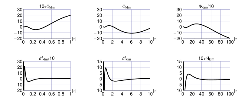
Figure 2: Analytic solutions (55) for the perturbations $\Phi_{klm}(\tau)$ and $\delta f_{klm}(\tau)$, using the simplified background functions $a(\tau)$ and $f(\tau)$ from (54). The parameters are $\{k,\,C_{klm},\,\alpha_{klm},\,f_{\text{bb}},\,d_{2}\}=\{2,\,2,\,0,\,1,\,1\}$.

III.4.3 Numerical results

For a preliminary numerical calculation, we use the following simplified background functions which have the correct global behavior:

$$a^{\text{(global-simplified-background)}}(\tau) = \tau\,,$$ (56a)

$$\overline{f}^{\text{(global-simplified-background)}}(\tau) = \frac{f_{\text{bb}}\,+f_{0}\,\tau^{2}}{1+\tau^{2}}\,.$$ (56b)

We then get the numerical $\Phi_{klm}(\tau)$ solution from (50a) with boundary conditions at $\tau=1$. For the sake of comparison, these boundary conditions at $\tau=1$ are taken to match the previous analytic function (55a) with $C_{klm}=2$ and $\alpha_{klm}=0$. Inserting that numerical $\Phi_{klm}(\tau)$ solution in (50b) gives the dimensionless $q$-field perturbation $\delta f_{klm}(\tau)$.

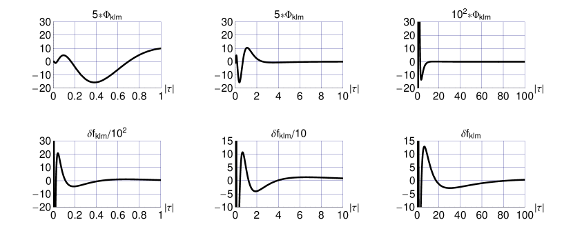
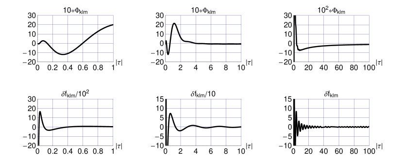
Figure 3: Numerical solution $\Phi_{klm}(\tau)$ from the ODE (50a) with boundary conditions $\Phi_{klm}(1)=2$ and $\dot{\Phi}_{klm}(1)=2$, for background functions $a(\tau)$ and $f(\tau)$ from (56). The dimensionless $q$-field perturbation $\delta f_{klm}(\tau)$ follows from the numerical $\Phi_{klm}(\tau)$ solution and (50b). The parameters are $\{k,\,f_{\text{bb}},\,f_{0}\}=\{2,\,1,\,1.51749\}$.

Figure 4: Numerical solution $\Phi_{klm}(\tau)$ from the ODE (50a) with boundary conditions $\Phi_{klm}(1)=2$ and $\dot{\Phi}_{klm}(1)=2$, for numerical background functions $a(\tau)$ and $f(\tau)$ from Fig. 1. The dimensionless $q$-field perturbation $\delta f_{klm}(\tau)$ follows from the numerical $\Phi_{klm}(\tau)$ solution and (50b). The parameters are $\{\lambda,\,k,\,f_{\text{bb}},\,f_{0}\}=\{1,\,2,\,1,\,1.51749\}$.

These preliminary numerical results are shown in Fig. 4. The qualitative behavior for $\tau\lesssim 1$ of Fig. 4 is similar to that of Fig. 2. New in Fig. 4 is that the $\Phi_{klm}$ oscillations essentially disappear for larger $\tau$ values, most likely, because the $\overline{f}(\tau)$ function from (56b) approaches its asymptotic equilibrium value $f_{0}$, instead of growing indefinitely as in (54b).

For the final numerical calculation, we use the numerical background functions $a(\tau)$ and $\overline{f}(\tau)$ from Fig. 1 to get the perturbations $\Phi_{klm}(\tau)$ and $\delta f_{klm}(\tau)$ from (50). These numerical results are shown in Fig. 4.

The qualitative behavior for $\tau\lesssim 10$ of Fig. 4 is similar to that of Fig. 4. New in Fig. 4 are the small $\delta f_{klm}(\tau)$ oscillations starting at $\tau\sim 2$, which are, most likely, due to the oscillations of the background field $\overline{f}(\tau)$ as it approaches the equilibrium value $f_{0}$ (see Fig. 1).

IV Discussion

In this article, we have, first, presented a simplified model for a time-symmetric Milne-like universe. In this simplified dynamic-vacuum-energy model, like in the previous model of Ref. KlinkhamerLing2019 , the big bang singularity is just a coordinate singularity Ling2018 with finite curvature and energy density. We have, then, calculated the dynamics of scalar metric perturbations.

The perturbation results of Fig. 4 can be described as follows: starting with small perturbations $\Phi_{klm}$ and $\delta f_{klm}$ at $\tau=-100$ and evolving them towards $\tau=0^{-}$, it is found that the $\delta f_{klm}$ oscillations get a larger and larger amplitude, so that perturbation theory breaks down (see App. A for related results on the perturbed Ricci curvature scalar). In short, the initial perturbations from $\tau=-100$ evolve and upset the unperturbed big bang solution $\tau=0^{-}$. Incidentally, with such a major disruption of the original big bang behavior, the discussion of possible cross-big-bang information transfer becomes moot.

At this moment, it may be worthwhile to compare our perturbation results of the Milne-like universe with those of the nonsingular bounce KlinkhamerWang2019-nonsing-bounce-pert . Specifically, the results for the scalar metric perturbations and the corresponding adiabatic perturbations of the nonrelativistic-matter energy density were found to be given by

$$\Phi_{\mathbf{k}}(t)\,\Big{|}^{\text{(nonsingular-bounce)}} = \widehat{C}_{\mathbf{k},\,1}+\frac{b^{5/3}\,\widehat{C}_{\mathbf{k},\,2}}{\big{(}b^{2}+t^{2}\big{)}^{5/6}}\,,$$ (57a)

$$\frac{\delta\rho_{\mathbf{k}}(t)}{\bar{\rho}(t)}\,\Big{|}^{\text{(nonsingular-bounce)}} = -\left[2+\frac{3}{2}\,|\mathbf{k}|^{2}\,\big{(}b^{2}+t_{0}^{2}\big{)}^{2/3}\,\big{(}b^{2}+t^{2}\big{)}^{1/3}\right]\widehat{C}_{\mathbf{k},\,1}$$ (57b)

$$+\left[3-\frac{3}{2}\,|\mathbf{k}|^{2}\,\big{(}b^{2}+t_{0}^{2}\big{)}^{2/3}\,\big{(}b^{2}+t^{2}\big{)}^{1/3}\right]\frac{b^{5/3}\,\widehat{C}_{\mathbf{k},\,2}}{\big{(}b^{2}+t^{2}\big{)}^{5/6}}\,,$$

where $b>0$ is the spacetime-defect length scale entering the metric Ansatz and $t_{0}$ an arbitrary reference time used for the background cosmic scale factor; see Ref. KlinkhamerWang2019-nonsing-bounce-pert for further details. The behavior of the perturbations (57) at the moment of the bounce, $t=0$, is perfectly regular due to the presence of the $b^{2}$ terms in the various denominators. This regular behavior of the nonsingular-bounce perturbations (57) contrasts with the essential-singularity behavior of the Milne-like-universe perturbations as shown in (55).

The heuristic explanation for the different behavior discussed in the previous paragraph may be twofold. First, the nonsingular bounce has a nonvanishing cosmic scale factor $a(t)$ at the bounce, whereas the Milne-like universe has a vanishing cosmic scale factor $a(t)$ at the big bang, which requires delicate cancellations in order to give a mere coordinate singularity and these cancellations may be destroyed by perturbations of the metric. Second, the nonsingular bounce has a “hard-wired” parameter $b$ to regularize the potential big bang singularity, whereas the Milne-like universe has a positive vacuum energy density, which traces back to a dynamic vacuum energy density $\rho_{V}(q)$.

This last problematic point of the Milne-like model would disappear if the variable quantity $\rho_{V}(q)$ were replaced by a positive cosmological constant $\Lambda$, but then the question resurfaces as how to remove the nonvanishing vacuum energy density as the universe evolves. More attractive would be to keep the dynamic vacuum energy density $\rho_{V}(q)$ and to find a mechanism that freezes $q(x)$ at $t=0$, which then forces having a vanishing perturbation $\delta q(x)=0$ at $t=0$ [this would effectively set $C_{klm}=0$ in (55)]. Such a freezing of the $q$-field has been discussed in a different context (cf. Sec. IV of Ref. KlinkhamerVolovik2009 ) and may indeed be the preferred way to rescue the big bang coordinate singularity of the Milne-like universe.

Appendix A Perturbed Ricci scalar

The Ricci curvature scalar from the perturbed spatially-hyperbolic Robertson–Walker metric (III.2) is given by:

$$R=\frac{1}{\Omega^{2}(\eta)}\left[6\,\left(\frac{\Omega^{\prime\prime}}{\Omega}-1\right)-54\,\Phi^{\prime\prime}-24\,\frac{\Omega^{\prime}}{\Omega}\,\Phi^{\prime}-12\,\frac{\Omega^{\prime\prime}}{\Omega}\Phi-12\,\Phi-46\,\nabla^{2}\,\Phi\right]+\text{O}\left(\Phi^{2}\right),$$ (58)

where the prime stands for differentiation with respect to $\eta$ and where (36) has been used. Changing to the original cosmic time coordinate $t$ from (27) and setting $\Omega(\eta)=a(t)$, we have

$$R=6\,\left(\frac{\ddot{a}}{a}+\frac{\dot{a}^{2}}{a^{2}}-\frac{1}{a^{2}}\right)-54\,\ddot{\Phi}-78\,\frac{\dot{a}}{a}\dot{\Phi}-12\,\left(\frac{\dot{a}^{2}}{a^{2}}+\frac{\ddot{a}}{a}\right)\Phi-12\,\frac{\Phi}{a^{2}}-46\,\frac{\nabla^{2}\Phi}{a^{2}}+\text{O}\left(\Phi^{2}\right),$$ (59)

where the overdot stands for differentiation with respect to $t$.

With the background function (54a) and the analytic $\Phi$ solution (55a), we then get the following first-order perturbation of the dimensionless Ricci curvature scalar ($\tau$ is the dimensionless version of the time coordinate $t$):

$$\delta R_{klm}(\tau) = \frac{C_{klm}}{\sqrt{\tau^{2}}}\Bigg{(}\left(100\,k^{2}-44\right)\,\cos\left[\alpha_{klm}+\frac{1}{2}\,k\,\log\left(\tau^{2}\right)\right]$$ (60)

$$+132\,k\,\sin\left[\alpha_{klm}+\frac{1}{2}\,k\,\log\left(\tau^{2}\right)\right]\Bigg{)}\,,$$

which displays the same type of behavior as found for $\delta f_{klm}(\tau)$ in Sec. III.4. In fact, the perturbation (60) ruins the regular behavior at $\tau=0$ of the background Ricci scalar (23a).

References

• (1) A.A. Friedmann, “Über die Krümmung des Raumes” (On the curvature of space), Z. Phys. 10, 377 (1922); “Über die Möglichkeit einer Welt mit konstanter negativer Krümmung des Raumes” (On the possibility of a world with constant negative curvature), Z. Phys. 21, 326 (1924).
• (2) S. Weinberg, Gravitation and Cosmology : Principles and Applications of the General Theory of Relativity (John Wiley and Sons, New York, 1972).
• (3) C.W. Misner, K.S. Thorne, and J.A. Wheeler, Gravitation (Princeton University Press, Princeton, NJ, 2017).
• (4) F.R. Klinkhamer, “Regularized big bang singularity,” Phys. Rev. D 100, 023536 (2019), arXiv:1903.10450.
• (5) F.R. Klinkhamer and Z.L. Wang, “Nonsingular bouncing cosmology from general relativity,” Phys. Rev. D 100, 083534 (2019), arXiv:1904.09961.
• (6) F.R. Klinkhamer and Z.L. Wang, “Asymmetric nonsingular bounce from a dynamic scalar field,” Lett. High Energy Phys. 3, 9 (2019), arXiv:1906.04708.
• (7) F.R. Klinkhamer, “Nonsingular bounce revisited,” arXiv:1907.06547.
• (8) F.R. Klinkhamer and Z.L. Wang, “Nonsingular bouncing cosmology from general relativity: Scalar metric perturbations,” arXiv:1911.06173.
• (9) E. Ling, “The big bang is a coordinate singularity for $k=-1$ inflationary FLRW spacetimes,” arXiv:1810.06789.
• (10) F.R. Klinkhamer and E. Ling, “Model for a time-symmetric Milne-like universe without big bang curvature singularity,” arXiv:1909.05816.
• (11) E.A.  Milne, “World structure and the expansion of the universe,” Nature (London) 130, 9 (1932).
• (12) N.D. Birrell and P.C.W. Davies, Quantum Fields in Curved Space (Cambridge University Press, Cambridge, England, 1982).
• (13) V. Mukhanov, Physical Foundations of Cosmology (Cambridge University Press, Cambridge, England, 2005).
• (14) F.R. Klinkhamer and G.E. Volovik, “Self-tuning vacuum variable and cosmological constant,” Phys. Rev. D 77, 085015 (2008), arXiv:0711.3170.
• (15) F.R. Klinkhamer and G.E. Volovik, “Dynamic vacuum variable and equilibrium approach in cosmology,” Phys. Rev. D 78, 063528 (2008), arXiv:0806.2805.
• (16) F.R. Klinkhamer and G.E. Volovik, “Vacuum energy density triggered by the electroweak crossover,” Phys. Rev. D 80, 083001 (2009), arXiv:0905.1919.
• (17) F R. Klinkhamer and G.E. Volovik, “Dynamic cancellation of a cosmological constant and approach to the Minkowski vacuum,” Mod. Phys. Lett. A 31, 1650160 (2016), arXiv:1601.00601.
• (18) F.R. Klinkhamer and G.E. Volovik, “Propagating $q$-field and $q$-ball solution,” Mod. Phys. Lett. A 32, 1750103 (2017), arXiv:1609.03533.
• (19) F.R. Klinkhamer and G.E. Volovik, “Dark matter from dark energy in $q$-theory,” JETP Lett. 105, 74 (2017), arXiv:1612.02326.
• (20) F.R. Klinkhamer and G.E. Volovik, “More on cold dark matter from q-theory,” arXiv:1612.04235.
• (21) F.R. Klinkhamer and T. Mistele, “Classical stability of higher-derivative $q$-theory in the four-form-field-strength realization,” Int. J. Mod. Phys. A 32, 1750090 (2017), arXiv:1704.05436.
• (22) F.R. Klinkhamer, O.P. Santillan, G.E. Volovik, and A. Zhou, “Vacuum energy decay from a q-bubble,” Physics 1, 321 (2019), arXiv:1901.05938.
• (23) V.F. Mukhanov, H.A. Feldman, and R.H. Brandenberger, “Theory of cosmological perturbations,” Phys. Rept.  215 (1992) 203.
• (24) N.Ya. Vilenkin and Ya.A. Smorodinsky, “Invariant expansions of relativistic amplitudes,” Sov. Phys. JETP 19, 1209 (1964).
• (25) H. Kodama and M. Sasaki, “Cosmological perturbation theory,” Prog. Theor. Phys. Suppl.  78, 1 (1984).
• (26) N.J. Cornish and D.N. Spergel, “On the eigenmodes of compact hyperbolic 3-manifolds,” arXiv:math/9906017.