Cavity

Optomagnonics

Silvia Viola Kusminskiy

Max Planck Institute for the Science of Light

Staudtstraße 2, 91058 Erlangen, Germany

and

Friedrich-Alexander University Erlangen-Nuremberg

Staudtstraße 7, 91058 Erlangen, Germany

Abstract

In the recent years a series of experimental and theoretical efforts have centered around a new topic: the coherent, cavity-enhanced interaction between optical photons and solid state magnons. The resulting emerging field of Cavity Optomagnonics is of interest both at a fundamental level, providing a new platform to study light-matter interaction in confined structures, as well as for its possible relevance for hybrid quantum technologies. In this chapter I introduce the basic concepts of Cavity Optomagnonics and review some theoretical developments.

Contents

1. 1 Introduction
2. 2 Optomagnonic Hamiltonian
   1. 2.1 Faraday Rotation
   2. 2.2 Optomagnonic coupling
      1. 2.2.1 Homogeneous magnon mode
      2. 2.2.2 Magnetic textures
   3. 2.3 Total Hamiltonian
      1. 2.3.1 Free Hamiltonian
      2. 2.3.2 Driving term
      3. 2.3.3 Total Hamiltonian for the Kittel mode
      4. 2.3.4 Total Hamiltonian and linearization
3. 3 Equations of Motion
   1. 3.1 Heisenberg equations of motion
   2. 3.2 Dissipative terms
      1. 3.2.1 Landau-Lifschitz-Gilbert equation of motion
      2. 3.2.2 Coupling to an external bath for the photon field
   3. 3.3 Light-induced dynamics of a classical macrospin
4. 4 Optomagnonics with a magnetic vortex
   1. 4.0.1 Magnetic vortex
   2. 4.0.2 Optomagnonic coupling for the gyrotropic mode
5. 5 A quantum protocol: all-optical magnon heralding
   1. 5.1 Hamiltonian and Langevin Equations of Motion
   2. 5.2 Write and read protocol
   3. 5.3 Solution of the linear quantum Langevin equations
   4. 5.4 Probability of heralding a magnon
   5. 5.5 Magnon cooling
6. 6 Outlook

Chapter 1 Introduction

The last two decades have seen enormous advances towards the realization of quantum technologies [1]. The ability to bring systems into the quantum regime, to design them, and to control them, can enable ultra-sensitive measurement and the manipulation of information at the quantum level, from quantum computers [2] to a quantum internet [3]. At the same time, it permits testing the predictions of quantum mechanics at unprecedented macroscopic scales [4].

Harnessing the power of quantum mechanics for applications implies being able to design a system for a certain desired quantum functionality. In general this means going beyond the single-atom limit, into the mesoscopic regime. Mesoscopic systems are comprised of millions of atoms and their behavior is described by collective excitations: e.g. the mechanical vibrations of a nanobeam. These systems, with characteristic length scales from tens of nanometers to hundreds of microns, are such that their collective excitations can be designed and brought into the quantum regime. This is however very challenging, since quantum states are fragile and require temperatures lower than the frequencies of the corresponding collective excitations. Breakthrough experiments in 2011 used active cooling to bring a macroscopic mode of mechanical vibration into its quantum ground state [5, 6], by using the backaction of electromagnetic radiation in a cavity. This is an example of cavity optomechanical systems [7]. Very generally, a cavity is a “box” which serves to confine the electromagnetic fields and can be used to enhance and even modify the interaction between electromagnetic radiation and matter. The field of cavity optomechanics has evolved rapidly, showing, for example, the possibility of entangling micrometer sized oscillators via the optomechanical interaction [8].

Cavity optomechanical systems form part of a broader class of systems denominated hybrid quantum systems [9]. These combine different degrees of freedom, such as photonic, mechanical, electronic, or magnetic, with the aim of controlling and optimizing their quantum functionality. For example, while quantum information can be processed with superconducting qubits at microwave frequencies [10], transmitting the information through long distances and at room temperature can be done with optical photons, due to their much higher frequencies. In turn, storing quantum information requires systems with long coherence times such that they can act as quantum memories. Promising results have been obtained in this regard using ensembles of spin impurities in a solid matrix [11].

In recent years, solid state magnetic systems have emerged as promising candidates for integrating them in hybrid quantum systems. Current research directions include spintronics [12], which aims at using the spin degree of freedom as a carrier replacing the electron, with the advantage of no energy loss due to Joule heating. Magnetic and electronic degrees of freedom couple well, and the concept of current-induced spin torque, proposed theoretically in 1996 [13], is being nowadays used in the development of random access memories [14]. The field of spin mechanics, in turn, deals with the coupling of the spin and mechanical degrees of freedom [15]. A hybrid spin mechanical system incorporating also an optomechanical cavity has been moreover demonstrated for ultra-sensitive magnetometry [16].

The interaction between electromagnetic radiation and magnetically ordered solid state systems in the context of hybrid quantum systems has however been an unexplored path until quite recently [17]. This changed with seminal experiments from 2013 to 2015, in which strong coherent coupling between microwave photons and magnons in Yttrium Iron Garnet (YIG) was demonstrated [18, 19, 20, 21], following a theoretical proposal in 2010 [22]. Magnons are the collective elementary excitations of magnetic systems, the quanta of the corresponding spin waves in the material. In these experiments, a microwave cavity was used to enhance the spin-photon interaction. The collective nature of the magnons, involving all spins in the magnetic sample, also provides a factor of enhancement to the magnon-photon coupling. The microwave field in the cavity can serve moreover as an intermediary field to couple the YIG magnons coherently to a superconducting qubit, indicating the potential of these magnetic systems for quantum information platforms [23]. In 2016, the first experimental [24, 25, 26] and theoretical [27, 28] works on cavity optomagnonics appeared, in which an optical cavity enhances the interaction between the spins and optical photons.

Since MW photons and the probed YIG magnons have similar energies in the GHz range, the magnon-phonon coupling can be tuned to be resonant, for example by applying an external magnetic field which controls the frequency of the magnonic excitations. The coupling term is of the form

$$g_{{\rm MW}}\left(\hat{S}^{+}\hat{a}^{\dagger}+\hat{S}^{-}\hat{a}\right)\,,$$ (1.0.1)

written in terms of the spin ladder operators $\hat{S}^{\pm}$ and the microwave photons operators $\hat{a}^{(\dagger)}$. The first term creates a photon in mode $\hat{a}$ by annihilating a magnon, and vice-versa for the second term. The coupling strength between magnons and photons $g_{{\rm MW}}$ is enhanced with respect to the single-spin coupling $g_{0}$ due to the collective character of the magnons by a factor $\sqrt{N}$, where $N$ is the number of spins participating in the magnon mode [22, 17]. MW cavity systems with magnetic elements can be by now routinely brought into the strong coherent coupling regime, with coupling strengths in the order of hundreds of ${\rm MHz}$ [29, 30, 31, 32, 33, 34]. In this regime, photons and magnons hybridize, forming a quasiparticle denominated a magnon polariton. Strong coupling is a prerequisite for quantum information manipulation, since it indicates the rate at which information is transferred between the different degrees of freedom. New routes towards tunability and quantum control [35, 36, 37, 38, 30, 39], and on-chip [31, 40, 41] realizations of these systems are also starting to be explored.

The frequency of optical photons is, on the other hand, in the range of hundred THz and the coupling to magnons is necessarily parametric, giving rise to inelastic Brillouin scattering [42]. In its simplest form, the coupling reads

$$g_{{\rm OP}}\hat{S}_{i}\hat{a}^{\dagger}\hat{a},$$ (1.0.2)

where $\hat{S}_{i}$ is the $i=x,\,y,\,{\rm or\,}z$ component of the spin operator and in this case optical photons operators $\hat{a}^{(\dagger)}$. The spin-photon coupling $g_{{\rm OP}}$ in this regime is inherently weak. The use of an optical cavity has been predicted to boost the interaction and, under certain conditions, to allow the system to enter in the strong coupling regime [27, 28, 43, 44, 45]. These conditions are however challenging, and the current experimental implementations are far from the strong coupling regime. In particular, given the weakness of the intrinsic interaction, optimal mode matching between magnon and photonic modes is required. Given the complexity of structured magnetic systems, this necessitates nontrivial theoretical design and challenging experimental implementation. The challenge makes for exciting times in cavity optomagnonics research [46, 44, 47, 48, 49, 50, 51, 52, 45]. It is to be expected that the shortcomings in the coupling will be overcome, opening the door to applications in quantum platforms. For example, magnons could be used as a quantum transducer, converting information up or down between MW and telecom photons.

Besides applications, cavity optomagnonics provides a unique setup in which concepts of cavity quantum electrodynamics (QED) can be applied to a magnetic system and its excitations. Originating from studying the electromagnetic radiation emission and absorption properties of single atoms in a cavity [53, 54, 55], cavity QED is nowadays a well-established framework to study light-matter interaction with confined electromagnetic fields. The concepts have been extended with great success to electromagnetic circuits [56] (circuit QED) and, as mentioned above, optomechanics. The extension to magnetic systems promises rich physics to discover.

The following sections cover the basics of cavity optomagnonics, restricted to the coupling of magnetic systems to photons in the optical domain. We derive the optomagnonic Hamiltonian starting from the Faraday rotation of light in magnetized solids and analyze in detail two solvable limits. In one case, we treat the interaction of light with the homogeneous magnon mode of the magnetic material (denominated the Kittel mode). For this mode, all spins precess in phase and they can be treated as a single degree of freedom, consisting of a macrospin. This allows for treating arbitrary dynamics of the macrospin, including nonlinear dynamics away for the equilibrium point. In the other case, we study the coupling to arbitrary magnon modes but restricted to the spin-wave limit, where only small deviations of the spins from their equilibrium can be treated. In this limit we can address the coherent interaction of light with magnetic textures. We will derive both the quantum Langevin and semiclassical equations of motion for the coupled open quantum system, and study the spin induced dynamics due to the light in the cavity. Finally, we will go over a proposal of a quantum protocol for creating non-classical macroscopic states of the magnetic system by using light.

Chapter 2 Optomagnonic Hamiltonian

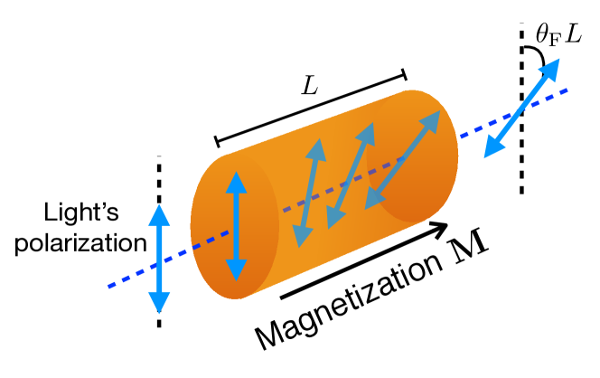
Cavity optomagnonic systems rely on the interaction between magnetic insulators and electromagnetic fields at optical frequencies. At these high frequencies, the magnetic permeability of the material can be taken as that of the vacuum, $\mu_{0}$, and the magneto-optical interaction modeled solely through the dielectric permittivity tensor, $\varepsilon_{ij}$ [57]. One is therefore interested in the coupling between the electric field component of the electromagnetic wave, and the magnetization of the host material. This coupling is responsible for the classical Faraday effect, where the plane of polarization of light is rotated as the light propagates through the magnetized medium, see Fig. (2.1.1). In this configuration, a linearly polarized plane wave propagates along the magnetization direction, and the resulting Faraday rotation of the polarization’s plane per unit length of propagation is given by $\theta_{{\rm F}}$, which is a characteristic of the material (sometimes the Faraday rotation is given in terms of the Verdet constant of the material, which is the angle of rotation per unit length, per unit magnetic field).

2.1 Faraday Rotation

The rotation of the plane of polarization of the light can be understood at a phenomenological level by noting that, if one writes the linear polarization in a circularly polarized basis, right and left polarizations inside of the material are not equivalent since time reversal symmetry is broken due to the magnetization $\mathbf{M}$. Effectively, this results on a different index of refraction for the two circular polarizations, which accumulates as a phase difference as light propagates, and results on the rotation of the polarization in the linear basis. This phenomenon is also known as magnetic circular birefringence and it is non-reciprocal, that is, the acquired phase adds up if the propagation direction is reversed.

Figure 2.1.1: Faraday rotation of linearly polarized light propagating through a magnetized material. The sketch shows the Faraday configuration, where the light propagates along the magnetization direction. After a length $L$, the plane of polarization has rotated an angle $\theta_{{\rm F}}L$ in the plane perpendicular to the propagation direction.

Using the zero energy loss condition, implying that no energy from the electromagnetic wave is absorbed in the material, together with the Onsager reciprocity condition for response functions in the presence of a magnetic field, one can derive symmetry conditions on the permittivity tensor of the magnetic material. The zero-loss condition is a good approximation for transparent media. One finds that the permittivity tensor (i) is Hermitian, (ii) its real part is symmetric in the magnetization, and (iii) its imaginary part is antisymmetric in the magnetization [58, 57, 59]. It is easy to see that a matrix of the form

$$\varepsilon_{ij}(\mathbf{M})=\varepsilon_{0}\left(\varepsilon_{r}\delta_{ij}-if\epsilon_{ijk}M_{k}\right)$$ (2.1.1)

where $\epsilon_{ijk}$ is the Levi-Civita tensor and $ijk$ are spatial indices, fulfills conditions (i) to (iii). Throughout this chapter we use the Einstein convention of summation over repeated indices. Eq. (2.1.1) assumes that the unmagnetized material is isotropic, this can, however, be readily generalized to non-isotropic materials by simply replacing $\varepsilon_{r}\delta_{ij}$ by the corresponding (symmetric and real) permittivity tensor. The linear dependence of Eq. (2.1.1) on the magnetization is valid as long as the correction of the magnetization on the permittivity is small $\left(fM\ll\varepsilon_{r}\right)$, which is usually the case. By considering a linearly polarized plane wave propagating along the material, it is straightforward to show that the permittivity from Eq. (2.1.1) leads to the Faraday rotation of light (see e.g. Ref. [59]). Denoting the saturation magnetization by $\mathbf{M}_{{\rm s}}$, $f$ is related to the Faraday rotation coefficient by the expression

$$\theta_{{\rm F}}=\frac{\omega}{2c\sqrt{\varepsilon_{r}}}fM_{{\rm s}}\,$$ (2.1.2)

where $c=1/\sqrt{\varepsilon_{0}\mu_{0}}$, $\omega$ is the angular frequency of the light, and the condition $fM_{{\rm s}}\ll\varepsilon_{r}$ has been used.

In optomagnonic systems, one is usually interested in coupling light to the excitations of the magnetically ordered ground state, and not to the ground state itself. From a classical point of view, these excitations are time-dependent deviations of the magnetization with respect to the ground state, in a collective, phase-locked way, and constitute spin waves. Their respective quanta are denominated magnons. Hence, in optomagnonics the usual configuration between the optical fields and the magnetization is not the one from Faraday’s original experiment, where the light propagates along the magnetization direction, but perpendicular to it. This configuration is denominated the Voigt configuration. The Faraday configuration can however also be probed and leads to interesting effects concerning angular momentum conservation rules, as discussed in Ref. [52] and also in the previous chapter of this book. In cavity optomagnonics, the optical fields form standing waves in a cavity, and part of the task is to optimize the coupling between the so-called optical spin density and the magnetic excitations, as we show below.

We are therefore interested in contributions to the permittivity tensor that are linear in the deviations of the magnetization $\mathbf{M}=\mathbf{M}_{0}+\delta\mathbf{M}$, where $\mathbf{M}_{0}$ is the ground state magnetization and $\delta\mathbf{M}$ the deviation. It is easy to see that terms quadratic in $\mathbf{M}$, not included in Eq. (2.1.1), also give linear contributions in $\delta\mathbf{M}$ [42]. The quadratic contribution in $\mathbf{M}$ to the permittivity gives rise to the Cotton-Mouton effect, also referred to as magnetic linear birefringence. In contrast to the Faraday effect, the Cotton-Mouton effect is reciprocal. In the simplest situation, the ground state magnetization is uniform and equal to the saturation magnetization, $\mathbf{M_{0}=}\mathbf{M}_{{\rm s}}$. Defining the $z$-axis along $\mathbf{M}_{{\rm s}}$, the deviations of the magnetization can be written as $\delta\mathbf{M=}(M_{x},M_{y},0)$. In this case, the only finite components of $\varepsilon_{ij}(\delta\mathbf{M)}$ to first order in $\delta\mathbf{M}$, including the Cotton-Mouton term, are given by

$$\varepsilon_{yz}(\delta\mathbf{M}) =\varepsilon_{zy}^{*}(\delta\mathbf{M})=-i\varepsilon_{0}fM_{x}+2\varepsilon_{0}g_{44}M_{y}M_{{\rm s}}$$ (2.1.3)

$$\varepsilon_{xz}(\delta\mathbf{M}) =\varepsilon_{zx}^{*}(\delta\mathbf{M})=i\varepsilon_{0}fM_{y}+2\varepsilon_{0}g_{44}M_{x}M_{{\rm s}}$$

where $g_{44}$ is the Cotton-Mouton coefficient related to the corresponding rotation angle per unit length

$$\theta_{{\rm CM}}=\frac{\omega}{2c\sqrt{\varepsilon_{r}}}g_{44}M_{{\rm s}}^{2}\,,$$ (2.1.4)

which can be obtained via linear birefringence measurements [57]. In the following we will discuss the optomagnonic coupling focusing only on the Faraday term, considering a permittivity tensor of the form given by Eq. (2.1.1). The extension to include Cotton-Mouton terms is however straightforward. From Eq. (2.1.3) one can see that these terms introduce an asymmetry in the couplings [28].

2.2 Optomagnonic coupling

If we consider a medium in the presence of time-dependent electromagnetic fields, we can define an internal energy by taking the time average of the instantaneous energy. For non-dispersive media the permittivity tensor is independent of frequency, and it can be shown that the averaged internal energy can be written as [58]

$$E_{{\rm EM}}=\frac{1}{4}\int{\rm d}V\sum_{ij}\left(\mathbf{E}_{i}^{*}\varepsilon_{ij}\mathbf{E}_{j}+\mathbf{H}_{i}^{*}\mu_{ij}\mathbf{H}_{j}\right)\,,$$ (2.2.1)

where $\mathbf{E}$ is the electric field, $\mathbf{H}$ the magnetic field, $\mu_{ij}$ the permittivity tensor, and we have used the complex representation of the fields, i.e. such that ${\rm Re}\left\{\mathbf{E}\right\}=1/2\left(\mathbf{E}^{*}+\mathbf{E}\right)$. It is straightforward to show that the expression Eq. (2.2.2) is real. The magnetization-dependent part of the permittivity introduces a correction to the electromagnetic energy. Considering for simplicity only the Faraday rotation term in the permittivity (see Eq. (2.1.1)), from Eq. (2.2.1) it is straightforward to show that this correction is given by

$$U_{{\rm MO}}=-\frac{i}{4}f\varepsilon_{0}\int{\rm d}\mathbf{r}\mathbf{M}(\mathbf{r})\cdot\left[\mathbf{E}^{*}(\mathbf{r})\times\mathbf{E}(\mathbf{r})\right]\,.$$ (2.2.2)

The cross product term is proportional to the optical spin density

$$\mathbf{S}_{{\rm light}}(\mathbf{r})=\frac{\varepsilon_{0}}{2i\omega}\left[\mathbf{E}^{*}(\mathbf{r})\times\mathbf{E}(\mathbf{r})\right]$$ (2.2.3)

implying the need of a non-trivial polarization of the optical field to obtain a finite coupling term.

One is usually interested in problems where the magnetization $\mathbf{M}$ has a dynamical part, $\mathbf{M}(\mathbf{r},t)=\mathbf{M}_{0}(\mathbf{r})+\delta\mathbf{M}(\mathbf{r},t)$, where $\delta\mathbf{M}(\mathbf{r},t)$ is the term due to the spin-wave excitations. The static ground state can be uniform ($\mathbf{M}_{0}(\mathbf{r})\equiv\mathbf{M}_{{\rm s}}$) if the sample is saturated by an external magnetic field, or also in the case of nanometer samples, where the exchange interaction is predominant and —for a ferromagnetic interaction—, sufficient to align all spins. In general, the interplay of exchange interactions and dipole-dipole interactions (or other type of interactions, such as Dzyalozinskii-Moriya [60]) gives rise either to the formation of domains in macroscopic samples, or to textured ground states for intermediate sizes (typically microns) [61], where the surface to volume ratio is large enough as to make the boundaries relevant for the minimization of the magnetostatic energy [62]. The formation of domains or textures have an exchange energy cost, but minimize stray fields. The relevant term for the optomagnonic coupling is the dynamical part of the magnetization $\delta\mathbf{M}(\mathbf{r},t)$. Therefore Eq. (2.2.2) implies that, besides a nontrivial polarization of the optical fields, the symmetry of the modes should be such that the integral is finite. In particular, the overlap between magnetic and optical modes should be maximized.

Quantizing Eq. (2.2.2) leads to the optomagnonic coupling Hamiltonian for ferromagnets [27]. The electric fields $\mathbf{E}(\mathbf{r},t)$ can be readily quantized in terms of bosonic creation $\hat{a}_{\xi}^{\dagger}$ and annihilation operators $\hat{a}_{\xi}$,

$$\mathbf{E}(\mathbf{r},t)\rightarrow\hat{\mathbf{E}}(\mathbf{r},t)=\frac{1}{2}\sum_{\text{$\xi$}}\left[\mathbf{E}_{\xi}(\mathbf{r})\hat{a}_{\xi}(t)+\mathbf{E}_{\xi}^{*}(\mathbf{r})\hat{a}_{\xi}^{\dagger}(t)\right]$$ (2.2.4)

where $\xi$ labels the corresponding optical mode including the polarization index. The mode functions $\mathbf{E}_{\xi}(\mathbf{r})$ satisfy the Helmholtz equation

$$\left(\nabla^{2}+n^{2}k_{0}^{2}\right)\mathbf{E}_{\xi}(\mathbf{r})=0\,,$$ (2.2.5)

where $n$ is the index of refraction of the medium and $k_{0}$ the vacuum wave vector. The mode functions are found from Eq. (2.2.5) together with appropriate boundary conditions for the geometry and material of the optical cavity [63]. The photon operators obey the usual bosonic commutation rules $\left[\hat{a}_{\xi},\hat{a}_{\xi^{\prime}}^{\dagger}\right]=\delta_{\xi\xi^{\prime}}$ ($\delta_{\xi\xi^{\prime}}$ the Dirac delta) and $\left[\hat{a}_{\xi},\hat{a}_{\xi^{\prime}}\right]=\left[\hat{a}_{\xi}^{\dagger},\hat{a}_{\xi^{\prime}}^{\dagger}\right]=0$.

The magnetization, in turn, can be quantized in terms of local spin operators $\hat{\mathbf{s}}_{\mathbf{r}}$ ($\mathbf{r}$ indicates the position of the spin) fulfilling locally the angular momentum algebra $\left[\hat{\mathbf{s}}_{\mathbf{r}}^{i},\hat{\mathbf{s}}_{\mathbf{r}}^{j}\right]=i\hbar\epsilon_{ijk}\hat{\mathbf{s}}_{\mathbf{r}}^{k}$ and commuting otherwise. The spin operators can be written exactly in terms of bosonic ones via a Holstein-Primakoff transformation. In order to preserve the algebra, however, this transformation is necessarily nonlinear and introduces extra interaction terms between magnons [59]. There are two cases that one can treat, up to a certain extent, analytically: (i) the uniform case, in which the ground state is uniform and one is interested in the homogeneous, $\mathbf{k}=0$ spin-wave mode, denominated the Kittel mode, and (ii) the general, spatial-dependent case in the spin-wave limit, valid for small deviations of the spins from their equilibrium configuration. We give the resulting form of the optomagnonic Hamiltonian for the two cases in the following.

2.2.1 Homogeneous magnon mode

We start with the homogeneous case (i), where both the ground state magnetization and the excitation are spatially independent: $\mathbf{M}(\mathbf{r},t)=\mathbf{M}_{{\rm s}}+\delta\mathbf{M}(t)$, with $\mathbf{M}_{{\rm s}}$ the uniform saturation magnetization. In this case, the magnetization can be quantized simply in terms of a macrospin $\hat{\mathbf{S}}$

$$\frac{\mathbf{M}}{M_{{\rm s}}}\rightarrow\frac{\hat{\mathbf{S}}}{S}\,,$$ (2.2.6)

where $S$ is the total spin of the considered system. This quantization scheme allows to retain the spin algebra and to treat fully the nonlinearity of the problem ($\delta\mathbf{M}(t)$ does not need to be small), but it is restricted to the homogeneous case. From Eqs. (2.2.4) and (2.2.2), using the substitution rule Eq. (2.2.6), the optomagnonic coupling Hamiltonian in this case reduces to [27]

$$\hat{H}_{MO}=\hbar\sum_{j\beta\gamma}\hat{S}_{j}G_{\beta\gamma}^{j}\hat{a}_{\beta}^{\dagger}\hat{a}_{\gamma}$$ (2.2.7)

with coupling constants

$$G_{\beta\gamma}^{j}=-i\frac{\varepsilon_{0}f\,M_{{\rm s}}}{4\hbar S}\xi\epsilon_{jmn}\int{\rm d}\mathbf{r}E_{\beta m}^{*}(\mathbf{r)}E_{\gamma n}(\mathbf{r})\,,$$ (2.2.8)

where the Greek indices label the optical modes, and the Roman indices label the spatial components ($x,\,y,\,z$). The factor $\xi\leq 1$ is a measure of the overlap between the Kittel mode and the corresponding optical modes, with $\xi=1$ corresponding to optimal mode-matching. The $G^{j}$ are hermitian matrices which in general cannot be simultaneously diagonalized. One sees that there are two possible kinds of processes: intra-mode coupling, given by the diagonal elements of $G^{j}$, and inter-mode coupling, given by the off-diagonal elements.

The coupling constants $G_{\beta\gamma}^{j}$ are uniquely determined once the normalization of the electromagnetic field is specified. We follow the normalization procedure common in optomechanical systems, where the electromagnetic field amplitude is normalized to one photon over the EM vacuum [64]. The normalization condition is given by $\hbar\omega_{\alpha}=\varepsilon_{0}\varepsilon\langle\alpha|\int d^{3}\mathbf{r}|\hat{\mathbf{E}}(\mathbf{r})|^{2}|\alpha\rangle-\varepsilon_{0}\varepsilon\langle 0|\int d^{3}\mathbf{r}|\hat{\mathbf{E}}(\mathbf{r})|^{2}|0\rangle$, where $|\alpha\rangle$ is a state with a single photon in mode $\alpha$, and $|0\rangle$ is the cavity vacuum. One obtains

$$\hbar\omega_{\alpha}=2\varepsilon_{0}\varepsilon\int d\mathbf{r}|\mathbf{E}_{\alpha}(\mathbf{r})|^{2}\,.$$ (2.2.9)

With this normalization, Eq. (2.2.8) reads

$$G_{\beta\gamma}^{j}=-i\frac{f\,M_{{\rm s}}}{8S\varepsilon}\sqrt{\omega_{\beta}\omega_{\gamma}}\xi\epsilon_{jmn}\frac{\int{\rm d}\mathbf{r}E_{\beta m}^{*}(\mathbf{r)}E_{\gamma n}(\mathbf{r})}{\sqrt{\int d\mathbf{r}|\mathbf{E}_{\beta}(\mathbf{r})|^{2}}\sqrt{\int d\mathbf{r}|\mathbf{E}_{\gamma}(\mathbf{r})|^{2}}}\,.$$ (2.2.10)

Figure 2.2.1: Schematic representation of the geometry for the calculation of the optomagnonic coupling to the Kittel mode, Eqs. (2.2.12) and (2.2.13). Adapted from Ref. [59].

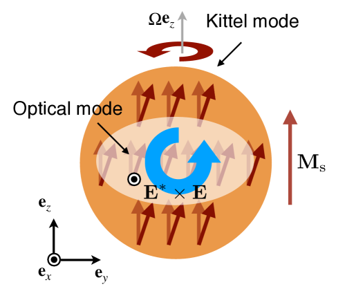
For processes involving a single optical mode, as we already pointed out, some degree of circular polarization of the mode is necessary for a finite coupling. Assuming an optical mode circularly polarized in the $yz$ plane, the optical spin density is along the $x$ axis and couples to the $x$ component of the spin operator, $\hat{S}_{x}$ (see Fig. (2.2.1)). The relevant coupling matrix is therefore $G_{\alpha\beta}^{x}$ which, in the considered geometry, is diagonal in the circularly polarized basis for the optical fields $\mathbf{e}_{{\rm R}/{\rm L}}=\left(\mathbf{e}_{y}\mp i\mathbf{e}_{z}\right)/\sqrt{2}$, as one can easily obtain from (2.2.8). We quantize the optical field for simplicity in terms of plane waves

$$\mathbf{E}(\mathbf{r},t)\rightarrow\mathbf{\hat{E}^{+}}(\mathbf{r},t) =i\sum_{{}_{j}}\mathbf{e}_{j}\sqrt{\frac{\omega}{2\varepsilon V}}\hat{a}_{j}(t)e^{i\mathbf{k_{j}\cdot r}}$$ (2.2.11)

$$\mathbf{E}^{*}(\mathbf{r},t)\rightarrow\mathbf{\hat{E}^{-}}(\mathbf{r},t) =-i\sum_{{}_{j}}\mathbf{e}_{j}\sqrt{\frac{\omega}{2\varepsilon V}}\hat{a}_{j}^{\dagger}(t)e^{-i\mathbf{k_{j}\cdot r}}\,,$$

where the $\pm$ superscripts follows the usual convention which indicates the positive and negative frequency components of the optical field, $\omega=\omega_{{\rm R}}=\omega_{{\rm L}}$, $j={\rm R},{\rm L}$ and $\mathbf{k}_{j}$ the corresponding wave vector. $V$ is the volume of the optical cavity. Using these expressions, one can easily show that Eq. (2.2.10) reduces to

$$G=G_{{\rm LL}}^{x}=-G_{{\rm RR}}^{x}=\frac{1}{S}\frac{c\theta_{{\rm F}}}{4\sqrt{\varepsilon}}\xi$$ (2.2.12)

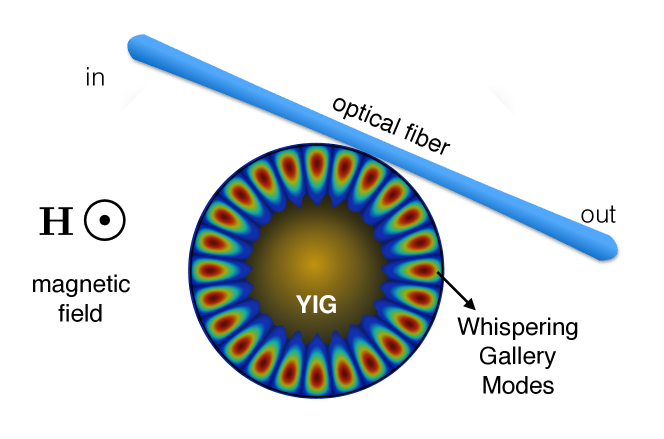
where we have used Eq. (2.1.2) to write $f$ in terms of $\theta_{{\rm F}}$. The numerical factor $\xi\leq 1$ takes into account the mode overlap of the electric field with the magnon mode and other geometric factors. In current optomagnonic experiments, involving YIG spheres, the optical modes in the cavity are actually whispering gallery modes (WGM), see Fig. (2.2.2). We will discuss a system with optical whispering gallery modes in Sec. (4), for now these details are hidden in $\xi$.

Considering Eqs. (2.2.7), (2.2.11), and (2.2.12), the coupling Hamiltonian reads [27]

$$\hat{H}_{MO}=\hbar\hat{S}_{x}G\left(\hat{a}_{L}^{\dagger}\hat{a}_{L}-\hat{a}_{R}^{\dagger}\hat{a}_{R}\right)\,.$$ (2.2.13)

In the spin-wave approximation, for small oscillations of the macrospin around its equilibrium position, we can replace the spin operator $\hat{S}_{x}$ by a position operator $\hat{S}_{x}\rightarrow\sqrt{S/2}(\hat{m}+\hat{m}^{\dagger})$ using a Holstein-Primakoff transformation truncated to first order in the bosonic operators (see Eq. (2.2.15)). In this limit,

$$\hat{H}_{MO}\approx\hbar\frac{1}{\sqrt{2S}}\frac{c\theta_{{\rm F}}}{4\sqrt{\varepsilon}}\xi\left(\hat{a}_{L}^{\dagger}\hat{a}_{L}-\hat{a}_{R}^{\dagger}\hat{a}_{R}\right)(\hat{m}+\hat{m}^{\dagger})$$ (2.2.14)

which is reminiscent of the Hamiltonian in the related field of cavity optomechanics, where light couples to mechanical vibrations by pressure forces. The coupling $g_{0}=G\sqrt{S/2}$ (given as an angular frequency) is a measure of the single photon-magnon coupling and equivalent to the vacuum coupling strength in optomechanics, where $g_{0}$ is proportional to the zero-point motion of the mechanical oscillator [7]. As we see from the dependence on $1/\sqrt{S}$ in Eq. (2.2.14), the single photon-magnon coupling is enhanced by small magnetic volumes.

The material of choice for optomagnonic systems is the insulating ferrimagnet YIG, due to the small losses both for the optics (absorption coefficient $\alpha\sim 0.069{\rm cm}^{-1}$ at $\lambda=1,2\,\mu{\rm m}$) and for the magnon modes (Gilbert damping coefficient $\eta_{{\rm G}}\approx 10^{-4}$) and large Faraday rotation ($\theta_{{\rm F}}=240\,{\rm deg}/{\rm cm}$ at $\lambda=1,2\,\mu{\rm m}$). Note that although YIG is technically a ferrimagnet, one magnetic sublattice is dominant and mostly behaves like a ferromagnet. The optical cavity is formed by the magnetic material itself, due to total internal reflection of light inside of the dielectric material. At optical frequencies, the index of refraction of YIG is $n=\sqrt{\varepsilon}\approx 2.24$, which combined with its low absorption makes it a reasonably good optical cavity if patterned appropriately. Experiments so far have used YIG spheres, since they are commercially available and relatively easy to polish into small sizes while preserving the quality of the optical cavity. Sizes nevertheless remain still too large, in the range of $100\mu{\rm m}$ radius. The YIG sphere supports optical modes in the way of whispering gallery modes which can be accessed through a tapered fiber, see the scheme of Fig. (2.2.2).

Assuming optimal mode-matching and a diffraction-limited volume of YIG of $1\mu{\rm m}^{3}$, one obtains $G\sqrt{S/2}\approx 0.1{\rm MHz}$ [27], which would be comparable to state of the art optomechanical systems [65]. Current experimental setups are still far from this limit, due to fabrication and design issues. Note for example that for the case of a sphere, the Kittel mode is a bulk mode, whereas the WGMs live near the surface, leading to a small overlap between the modes. Improving the current values of the coupling is however highly desirable for applications in the quantum regime.

Figure 2.2.2: Sketch of a YIG sphere supporting optical WGM. Within the material, photons and magnons interact via the optomagnonic interaction. The frequency of the magnons can be controlled by an external magnetic field $\mathbf{H}$ and the optical modes can be driven and probed by an optical fiber, which couples evanescently to the WGM.

2.2.2 Magnetic textures

One alternative to improve the value of the optomagnonic coupling is to go beyond the Kittel mode, searching for modes that would be better suited for mode matching with the optics. This is starting to be explored both theoretically [66, 44, 45] and experimentally [50, 49]. This brings us to case (ii) from our two limiting cases, where one allows for non-uniform ground states (also called magnetic textures) and/or magnetic excitations with a spatial structure, and uses the Holstein-Primakoff transformations to represent the excitations in terms of bosonic operators $\hat{m}_{i}$, where $i$ is the lattice site:

$$\hat{S}_{i}^{+} =\sqrt{2s}\sqrt{1-\frac{\hat{m}_{i}^{\dagger}\hat{m}_{i}}{2s}}\hat{m}_{i}$$

$$\hat{S}_{i}^{-} =\sqrt{2s}\hat{m}_{i}^{\dagger}\sqrt{1-\frac{\hat{m}_{i}^{\dagger}\hat{m}_{i}}{2s}}$$

$$\hat{S}_{i}^{z} =\left(s-\hat{m}_{i}^{\dagger}\hat{m}_{i}\right)\,.$$ (2.2.15)

In these, $s$ is the total spin per lattice site $i$, so that the total spin is given by $S=Ns$ with $N$ the number of lattice sites, and $\hat{S}_{i}^{\pm}=\hat{S}_{i}^{x}\pm i\hat{S}_{i}^{y}$ are the spin ladder operators. Eqs. (2.2.15) assume a quantization axis along the $z$ direction. If the magnetic ground state is textured, the quantization axis is local, defined by $\mathbf{e}_{z}(\mathbf{r})=\mathbf{M}_{{\rm s}}(\mathbf{r})/M_{{\rm s}}$. The bosonic operators $\hat{m}_{i}$ fulfill the usual bosonic commutation rules

$$\left[\hat{m}_{i},\,\hat{m}_{j}^{\dagger}\right] =\delta_{ij}$$ (2.2.16)

$$\left[\hat{m}_{i},\,\hat{m}_{j}\right] =\left[\hat{m}_{i}^{\dagger},\,\hat{m}_{j}^{\dagger}\right]=0\,.$$

The problem is simplified by cutting off the Holstein-Primakoff transformation to first order in the bosonic operators,

$$\hat{S}_{i}^{+} \approx\sqrt{2S}\hat{m}_{i}$$ (2.2.17)

$$\hat{S}_{i}^{-} \approx\sqrt{2S}\hat{m}_{i}^{\dagger}$$

$$\hat{S}_{i}^{z} \approx S\,,$$

and is therefore a linear approximation for the local spin operators, which are treated as harmonic oscillators. The elementary magnetic excitations are collective, since given a spin Hamiltonian (e.g. the Heisenberg Hamiltonian), after performing the approximation Eq. (2.2.17) one still needs to bring the Hamiltonian to a diagonal form, so that is is a sum of independent harmonic oscillators (e.g. in the bulk by going to Fourier space, $\hat{m}_{\mathbf{k}}$). These collective excitations are denominated magnons: essentially, one magnon is a “flipped” spin which is shared by the whole system. Higher-order terms in the expansion can be included and represent magnon-magnon interactions.

The quantization of the coupling term Eq. (2.2.2) in this case follows by writing the excitation $\delta\mathbf{M}(\mathbf{r},t)$ in terms of the magnon modes (by magnon modes we mean the bosonic operators which diagonalize the magnetic Hamiltonian). It is convenient to work in terms of the normalized magnetization $\delta\mathbf{m}(\mathbf{r},t)=\delta\mathbf{M}(\mathbf{r},t)/M_{{\rm s}}$. For small deviations $|\delta\mathbf{m}|\ll 1$ we can quantize the spin wave in analogy to Eq. (2.2.4) for the electric fields, by the substitution

$$\delta\mathbf{m}(\mathbf{r},t)\rightarrow\frac{1}{2}\sum_{\gamma}\left[\delta\mathbf{m}_{\gamma}(\mathbf{r})\hat{m}_{\gamma}+\delta\mathbf{m}_{\gamma}^{*}(\mathbf{r})\hat{m}_{\gamma}^{\dagger}\right]\,,$$ (2.2.18)

where $\hat{m}_{\gamma}^{(\dagger)}$ annihilates (creates) a magnon in mode $\gamma$. The information on its spatial structure is contained in the mode functions $\delta\mathbf{m}_{\gamma}(\mathbf{r})$. Together with Eq. (2.2.4), from Eq. (2.2.2) and using Eq. (2.1.2) we obtain the optomagnonic coupling Hamiltonian linearized in the spin fluctuations [44]

$$\hat{H}_{MO}=\hbar\sum_{\alpha\beta\gamma}G_{\alpha\beta\gamma}\hat{a}_{\alpha}^{\dagger}\hat{a}_{\beta}\hat{m}_{\gamma}+\hbar\sum_{\alpha\beta\gamma}G_{\alpha\beta\gamma}^{{\rm*}}\hat{a}_{\beta}^{\dagger}\hat{a}_{\alpha}\hat{m}_{\gamma}^{\dagger}$$ (2.2.19)

where

$$G_{\alpha\beta\gamma}=-i\frac{\theta_{{\rm F}}\lambda_{n}}{4\pi}\frac{\varepsilon_{0}\varepsilon}{2\hbar}\int{\rm d}\mathbf{r}\,\delta\mathbf{m}_{\gamma}(\mathbf{r})\cdot[\mathbf{E_{\alpha}^{*}}\left(\mathbf{r}\right)\times\mathbf{E}_{\beta}\left(\mathbf{r}\right)]$$ (2.2.20)

is the optomagnonic coupling in terms of the Faraday rotation per wavelength of the light in the material $\lambda_{n}=\lambda_{0}/n$, with $\lambda_{0}$ the vacuum wavelength. For YIG one obtains $\theta_{{\rm F}}\lambda_{n}/2\pi\approx 10^{-5}$. Within the linear regime for the spins, Eq. (2.2.21) is very general and allows to treat arbitrary geometries and modes, both optical and magnetic.

In Eq. (2.2.20) one still needs to specify the normalization of the modes. For the optical fields the normalization was given in Eq. (2.2.9). For the magnon modes, we impose a total magnetization corresponding to one Bohr magneton (times the corresponding gyromagnetic factor $g$) in the excitation. This normalizes the coupling to one magnon. From the definition Eq. (2.2.18), this is equivalent to imposing [44]

$$\frac{1}{4}\int{\rm d}\mathbf{r}\,|\delta\mathbf{m}_{\gamma}(\mathbf{r})|^{2}=\frac{g\mu_{{\rm B}}}{M_{{\rm s}}}\,.$$ (2.2.21)

The normalized coupling therefore reads

$$G_{\alpha\beta\gamma} =-i\frac{\theta_{{\rm F}}\lambda_{n}}{4\pi}\frac{1}{2}\sqrt{\frac{g\mu_{{\rm B}}}{M_{{\rm s}}}}\sqrt{\omega_{\beta}\omega_{\alpha}}$$ (2.2.22)

$$\times\frac{\int{\rm d}\mathbf{r}\,\delta\mathbf{m}_{\gamma}(\mathbf{r})\cdot[\mathbf{E_{\alpha}^{*}}\left(\mathbf{r}\right)\times\mathbf{E}_{\beta}\left(\mathbf{r}\right)]}{\sqrt{\int{\rm d}\mathbf{r}\,|\delta\mathbf{m}_{\gamma}(\mathbf{r})|^{2}}\sqrt{\int d\mathbf{r}|\mathbf{E}_{\beta}(\mathbf{r})|^{2}}\sqrt{\int d\mathbf{r}|\mathbf{E}_{\alpha}(\mathbf{r})|^{2}}}\,.$$

For the optical fields, it is common to define an effective mode volume $V_{{\rm E}}^{\alpha}$

$$V_{{\rm E}}^{\alpha}=\frac{\int d^{3}\mathbf{r}|\mathbf{E}_{\alpha}(\mathbf{r})|^{2}}{\max\left\{|\mathbf{E}_{\alpha}(\mathbf{r})|^{2}\right\}}\,,$$ (2.2.23)

which for a homogeneous electric field reduces simply to the volume occupied by the field. Analogously, we can define an effective magnetic volume

$$V_{{\rm M}}^{\gamma}=\frac{\int d^{3}\mathbf{r}|\delta\mathbf{m}_{\gamma}(\mathbf{r})|^{2}}{\max\left\{|\delta\mathbf{m}_{\gamma}(\mathbf{r})|^{2}\right\}}\,,$$ (2.2.24)

according to which

$$G_{\alpha\beta\gamma}=-i\frac{\theta_{{\rm F}}\lambda_{n}}{4\pi}\frac{1}{2}\sqrt{\frac{g\mu_{{\rm B}}}{M_{{\rm s}}}}\frac{\sqrt{\omega_{\beta}\omega_{\alpha}}}{\sqrt{V_{{\rm M}}^{\gamma}V_{{\rm E}}^{\alpha}V_{{\rm E}}^{\beta}}}\frac{\int{\rm d}\mathbf{r}\,\delta\mathbf{m}_{\gamma}(\mathbf{r})\cdot[\mathbf{E_{\alpha}^{*}}\left(\mathbf{r}\right)\times\mathbf{E}_{\beta}\left(\mathbf{r}\right)]}{|\delta\mathbf{m}_{\gamma}(\mathbf{r_{{\rm m}}})||\mathbf{E}_{\alpha}(\mathbf{r_{{\rm m}}})||\mathbf{E}_{\beta}(\mathbf{r_{{\rm m}}})|}\,,$$ (2.2.25)

where for simplicity of notation we have defined $\mathbf{r_{{\rm m}}}$ such that $|\mathbf{\delta\mathbf{m}_{\gamma}}(\mathbf{r_{{\rm m}}})|=\max\left\{|\mathbf{\delta\mathbf{m}_{\gamma}}(\mathbf{r})|\right\}$ and analogously for $\mathbf{E_{\alpha}}$.

From Eq. (2.2.25) we see that the strength of the coupling is cut off by the smallest volume in the integral factor. Assuming similar effective mode volumes for the optical fields, $V_{{\rm E}}^{\alpha}\equiv V_{{\rm E}}^{\alpha}\approx V_{{\rm E}}^{\beta}$, if $V_{{\rm M}}^{\gamma}\leq V_{{\rm E}}^{\alpha}$ the coupling is suppressed by a factor $\sqrt{V_{{\rm M}}^{\gamma}}/V_{{\rm E}}^{\alpha}$, favoring small optical volumes. For $V_{{\rm M}}^{\gamma}\geq V_{{\rm E}}^{\alpha}$ instead, the coupling goes as $1/\sqrt{V_{{\rm M}}^{\gamma}}$, favoring small magnetic volumes. Recalling that

$$M_{{\rm s}}=\frac{Sg\mu_{B}}{V_{{\rm M}}^{\gamma}}$$ (2.2.26)

where $S=Ns$ is the total spin in the volume $V_{{\rm M}}^{\gamma}$ ($N$ number of spins, $s$ spin value), we recover in this case the behavior $\propto 1/\sqrt{S}$ found above for the Kittel mode in the spin-wave approximation. From these scaling arguments, we see that small mode volumes and optimal mode matching are required for large coupling. In Sec. (4) we will use Eq. (2.2.25) to calculate the optomagnonic coupling in a cavity system consisting of a micromagnetic disk.

2.3 Total Hamiltonian

In the previous section, we derived the Hamiltonian that governs the coupling between optical photons and magnons in a cavity. In order to study dynamical processes, we need the total Hamiltonian of the system. Besides the coupling Hamiltonian, we need to include the free Hamiltonian both for magnons and photons (the kinetic terms). The cavity is an open system, which can be driven and is also subject to dissipation, both for magnons and photons. We can include the driving term in the Hamiltonian, the dissipation terms we will include at the level of the equations of motion in Sec. (3).

2.3.1 Free Hamiltonian

The total optomagnonic Hamiltonian $\hat{H}$ consists of the optomagnonic coupling term, given by either Eqs. (2.2.7) and (2.2.8) or Eqs.(2.2.19) and (2.2.20), plus the free photon Hamiltonian

$$\hat{H}_{{\rm ph}}=\hbar\sum_{\alpha}\omega_{\alpha}\hat{a}_{\alpha}^{\dagger}\hat{a}_{\alpha}$$ (2.3.1)

and the free magnetic term $\hat{H}_{{\rm m}}$. For the Kittel mode (case (i) from the previous section), this free term is simply the Larmor precession of the macrospin $\hat{\mathbf{S}}$,

$$\hat{H}_{{\rm m}}^{{\rm K}}=-\hbar\Omega\hat{S}_{z}\,,$$ (2.3.2)

where we have assumed an external magnetic field $\mathbf{B_{0}}$ applied along the $\hat{\mathbf{e}}_{z}$ axis and $\Omega$ is the free precession frequency of the macrospin, see Fig. (2.2.1). We assume also that the ground state magnetization is saturated and along $\hat{\mathbf{e}}_{z}$. The frequency $\Omega$ is in general controlled by $\mathbf{B_{0}}$. In the case of a spherical magnet, due to the high symmetry of the system $\Omega$ is independent of the demagnetization fields [62], and given simply by

$$\hbar\Omega_{{\rm sphere}}=|g\mu_{{\rm B}}B_{0}|\,.$$ (2.3.3)

For YIG, $g=2$ and the gyromagnetic factor equals that of the electron: $|\gamma_{{\rm e}}|=|g\mu_{{\rm B}}/\hbar|=1.76\times 10^{11}{\rm rad}/{\rm s}\cdot{\rm T}$. Applied magnetic fields in the range of tens of ${\rm mT}$ therefore lead to frequencies in the ${\rm GHz}$ range. For other geometries, e.g. ellipsoids or thin films, $\Omega$ depends also on the demagnetization fields which can be taken into account through demagnetization factors [67].

For general magnon modes in the spin-wave approximation (case (ii)), one writes the free magnetic term also as a sum of harmonic oscillators

$$\hat{H}_{{\rm m}}^{SW}=\hbar\sum_{\beta}\Omega_{\beta}\hat{m}_{\beta}^{\dagger}\hat{m}_{\beta}$$ (2.3.4)

where $\Omega_{\beta}$ is the dispersion of the $\beta$ magnon mode. Part of the problem in confined geometries is finding the magnon modes and corresponding dispersion, and, except for very simple geometries, micromagnetic simulations must be employed. Note that by using the Holstein-Primakoff expression for $\hat{S}_{z}$, c.f. Eq. (2.2.15), Eq. (2.3.2) reduces, asides from a constant, to an expression like Eq. (2.3.4).

2.3.2 Driving term

The cavity system can be driven by an external laser. The magnon modes can in principle also be driven by an external MW field, but we will not consider this in the following. The driving term can be included in the Hamiltonian as

$$\hat{H}_{{\rm{\rm D}}}=i\epsilon_{\alpha}(\hat{a}_{\alpha}e^{i\omega_{L}t}-\hat{a}_{\alpha}^{\dagger}e^{-i\omega_{L}t})\,,$$ (2.3.5)

where $\alpha$ indicates the mode that is being driven, $\omega_{L}$ is the laser frequency and

$$\epsilon_{\alpha}=\hbar\sqrt{\frac{2\kappa_{\alpha}\mathcal{P}_{\alpha}}{\hbar\omega_{L}}}$$ (2.3.6)

depends on the driving laser power $\mathcal{P}_{\alpha}$ and on the cavity decay rate $\kappa_{\alpha}$ of the pumped mode due to the coupling to the the driving channel, e.g. an optical fiber or waveguide. It is common to work in a rotating frame at the laser frequency $\omega_{L}$, so that the trivial time dependence $e^{i\omega_{L}t}$ is removed. This is achieved by the unitary transformation $\hat{U}=e^{-i\omega_{L}t\hat{a}_{\alpha}^{\dagger}\hat{a}_{\alpha}}$ under which the Hamiltonian transforms as $\hat{H}\rightarrow\hat{U}\hat{H}\hat{U}^{\dagger}-i\hbar\hat{U}\frac{\partial\hat{U}^{\dagger}}{\partial t}$. In the rotating frame, for a single photon mode $\alpha$ one obtains

$$\hat{H}_{{\rm ph}}+\hat{H}_{{\rm{\rm D}}}\rightarrow-\hbar\Delta_{\alpha}\hat{a}_{\alpha}^{\dagger}\hat{a}_{\alpha}+i\epsilon_{\alpha}(\hat{a}_{\alpha}-\hat{a}_{\alpha}^{\dagger})$$ (2.3.7)

where $\Delta_{\alpha}=\omega_{{\rm L}}-\omega_{\alpha}$ is the detuning of the driving laser frequency with respect to the resonance frequency of the optical cavity for the $\alpha$-mode. The generalization to multiple driven modes is straightforward. If $\Delta_{\alpha}>0$ ($\Delta_{\alpha}<0$ ) the system is said to be blue (red) detuned. In the literature, it is usual to write the Hamiltonian in the rotating frame omitting the driving term (second term on the RHS of Eq. (2.3.7)). In that case, the driving term is added at the level of the equations of motion, together with the dissipation and fluctuation terms.

2.3.3 Total Hamiltonian for the Kittel mode

The total cavity optomagnonic Hamiltonian, in the rotating frame and omitting the driving and dissipation terms, are given in the following both for the Kittel mode (case (i)) and in the spin-wave approximation (case (ii)). For the Kittel mode we choose a simplified model in which the light is circularly polarized in the $yz$ plane giving rise to the coupling in Eq. (2.2.13). Hence

$$\hat{H}_{{\rm K}}=-\hbar\Delta\hat{a}^{\dagger}\hat{a}-\hbar\Omega\hat{S}_{z}+\hbar G\hat{S}_{x}\hat{a}^{\dagger}\hat{a}$$ (2.3.8)

with $G$ given by Eq. (2.2.12). Since in this simple case the Hamiltonian is diagonal in the circularly polarized basis, right and left handed modes are not coupled and we can restrict the Hamiltonian to a single photon mode, which we denote with the operator $\hat{a}$ (compare with Eq. (2.2.13)). Note also that, as long as we work with the Voigt geometry, we can always find a system of coordinates such that the Hamiltonian can be expressed as in Eq. (2.3.8). The Hamiltonian in Eq. (2.3.8) seems deceptively simple, since, as we will see below, it leads to rich nonlinear dynamics even in the classical limit. The parametric coupling in the photon operators (the coupling is a two-photon process) gives rise to nonlinearities even in the spin-wave approximation. These are equivalent to the nonlinear behavior present in optomechanical systems [7]. Retaining the full macrospin dynamics introduces new nonlinear behavior unique to optomagnonic systems.

2.3.4 Total Hamiltonian and linearization

In the spin-wave approximation the total Hamiltonian reads

$$\hat{H}_{{\rm SW}}=-\hbar\sum_{\alpha}\Delta_{\alpha}\hat{a}_{\alpha}^{\dagger}\hat{a}_{\alpha}+\hbar\sum_{\beta}\Omega_{\beta}\hat{m}_{\beta}^{\dagger}\hat{m}_{\beta}+\hbar\sum_{\alpha\beta\gamma}G_{\alpha\beta\gamma}\hat{a}_{\alpha}^{\dagger}\hat{a}_{\beta}\hat{m}_{\gamma}+{\rm h.c.\,}$$ (2.3.9)

with $G_{\alpha\beta\gamma}$ given in Eq. (2.2.25). This Hamiltonian is a three-particle interacting Hamiltonian. Diagonalization is possible by linearizing the optical fields around the steady state solutions,

$$\hat{a}_{\alpha}= \langle\hat{a}_{\alpha}\rangle+\delta\hat{a}_{\alpha}$$ (2.3.10)

such that ${\rm d}\langle\hat{a}_{\alpha}\rangle/{\rm d}t=0$ and all the dynamics is contained in the fluctuation fields $\delta\hat{a}_{\alpha}$. The input laser power determines the average number of photons circulating in the cavity in mode $\alpha$, $n_{\alpha}=|\langle\hat{a}_{\alpha}\rangle|^{2}$. Considering terms up to linear order in the fluctuations $\delta\hat{a}_{\alpha}$, Eq. (2.3.9) reduces to a quadratic Hamiltonian

$$\hat{H}_{{\rm fl}} =-\hbar\sum_{\alpha}\Delta_{\alpha}\hat{a}_{\alpha}^{\dagger}\hat{a}_{\alpha}+\hbar\sum_{\beta}\Omega_{\beta}\hat{m}_{\beta}^{\dagger}\hat{m}_{\beta}$$ (2.3.11)

$$+\hbar\sum_{\alpha\beta\gamma}G_{\alpha\beta\gamma}\left(\sqrt{n_{\alpha}}\delta\hat{a}_{\beta}\hat{m}_{\gamma}+\sqrt{n_{\beta}}\delta\hat{a}_{\alpha}^{\dagger}\hat{m}_{\gamma}\right)+{\rm h.c.}\,.$$

This kind of Hamiltonian is well know from quantum optics and related systems (see e.g. Refs. [68, 7]), and it can be turned into a parametric amplifier ($\delta\hat{a}_{\beta}\hat{b}_{\gamma}$ and $\hat{m}_{\gamma}^{\dagger}\delta\hat{a}_{\beta}^{\dagger}$ terms) or a beam splitter Hamiltonian ($\delta\hat{a}_{\beta}\hat{m}_{\gamma}$ and $\hat{m}_{\gamma}^{\dagger}\delta\hat{a}_{\beta}^{\dagger}$) by tuning the external laser driving frequency. The combination

$$G_{{\rm eff}}=\sqrt{n}G$$ (2.3.12)

(with indices as appropriate) shows that the coupling $G$ is enhanced by the square root of the number of photons trapped in the cavity, and can in this way be controlled.

Chapter 3 Equations of Motion

In this section we split again for simplicity the discussion into the two cases (i) and (ii) detailed above. We will obtain the equations of motion for the macrospin dynamics, only valid for the Kittel mode but retaining the spin algebra and the full non-linearity of the problem, and and the spin-wave approximation, where we restrict the problem to the dynamics of coupled harmonic oscillators.

3.1 Heisenberg equations of motion

The Heisenberg equation of motion for an operator $\hat{\mathbf{O}}$ evolving under a Hamiltonian $\hat{H}$ is given by

$$\hbar\frac{d\hat{\mathbf{O}}}{dt} =i[\hat{H},\hat{\mathbf{O}}]\,.$$ (3.1.1)

In the macrospin approximation using $\hat{H}_{{\rm K}}$ given in Eq. (2.3.8) and imposing the commutation relations$\left[\hat{a},\hat{a}^{\dagger}\right]=1$, $\left[\hat{S}_{i},\hat{S}_{j}\right]=i\epsilon_{ijk}\hat{S}_{k}$ one obtains the following coupled equations of motion for the macrospin and the light field

$$\dot{\hat{a}} =-i\left(G\hat{S}_{x}-\Delta\right)\hat{a}$$ (3.1.2)

$$\dot{\mathbf{\hat{\mathbf{S}}}} =\left(G\hat{a}^{\dagger}\hat{a}\mathbf{\,e}_{x}-\Omega\,\mathbf{e}_{z}\right)\times\hat{\mathbf{S}}\,.$$

In the spin wave approximation, considering a general multimode system given by the Hamiltonian in Eq. (2.3.9) we obtain

$$\dot{\hat{a}}_{\alpha} =i\Delta_{\alpha}\hat{a}_{\alpha}-i\sum_{\beta\gamma}G_{\alpha\beta\gamma}\hat{a}_{\beta}\hat{m}_{\gamma}-i\sum_{\beta\gamma}G_{\beta\alpha\gamma}^{*}\hat{a}_{\beta}\hat{m}_{\gamma}^{\dagger}$$

$$\dot{\hat{m}}_{\gamma} =-i\Omega_{\gamma}\hat{m}_{\gamma}-i\sum_{\alpha\beta}G_{\alpha\beta\gamma}^{*}\hat{a}_{\beta}^{\dagger}\hat{a}_{\alpha}\,,$$ (3.1.3)

and analogously for $\hat{a}_{\alpha}^{\dagger}$ and $\hat{m}_{\gamma}^{\dagger}$. Eqs. (3.1.2) and (3.1.3) are written in a rotating frame but do not contain either driving or dissipative terms, we will include these below. For now, we note that for $G=0$ Eqs. (3.1.2) decouple into a simple harmonic oscillator for the optical field, and a Larmor precession equation for the spin operator. In particular, the equation of motion for the spin in this case is $\dot{\mathbf{\hat{\mathbf{S}}}}=-\Omega\,\mathbf{e}_{z}\times\hat{\mathbf{S}}$, which reduces to the well known Landau-Lifschitz equation of motion for the magnetization by taking the classical expectation values and proper rescaling. Note that the Landau-Lifschitz equation of motion is therefore semiclassical, since it is derived as the classical limit of the Heisenberg equation of motion.

3.2 Dissipative terms

The dissipative rates in cavity systems are very important since they determine how fast information in the system is lost to the environment. A very important figure of merit in hybrid systems is the cooperativity $\mathcal{C}$, which is defined as the ratio of the effective coupling strength (see Eq. (2.3.12)) to the decay channels in the system, in our case the photon decay rate $\kappa$ and the magnon decay rate which we take as $\Gamma=\Omega\eta_{{\rm G}}$,

$$\mathcal{C}=4\frac{G_{{\rm eff}}^{2}}{\kappa\Gamma}\,.$$ (3.2.1)

Quantum protocols require at least $\mathcal{C}>1$, so that information transfer can occur before the information is lost. Coherent state transfer between magnons and photons requires moreover that $\mathcal{C}/n_{{\rm tm}}>1$, where $n_{{\rm tm}}$ is the number of thermal magnons (the photon environment can be safely assumed to be at zero temperature for optical photons, since $k_{{\rm B}}T\ll\omega_{{\rm ph}}$).

3.2.1 Landau-Lifschitz-Gilbert equation of motion

To recover the classical dynamics of the spin, it is still necessary to include dissipation. This is done phenomenologically by adding a Gilbert damping term to the Landau-Lifschitz equation

$$\dot{\mathbf{S}}=-\Omega\,\mathbf{e}_{z}\times\mathbf{S}+\frac{\eta_{{\rm G}}}{S}(\mathbf{\dot{S}}\times\mathbf{S})$$ (3.2.2)

where $\eta_{{\rm G}}$ is a characteristic of the magnetic material and denominated the Gilbert damping coefficient. For YIG, $\eta_{{\rm G}}\approx 10^{-4}$, which is very low when compared to other magnetic materials. The Eq. (3.2.2) for the classical macrospin is denominated the Landau-Lifschitz-Gilbert equation of motion. Note that the dissipative term damps the precession of the spin, but does not alter the norm of the vector.

3.2.2 Coupling to an external bath for the photon field

The optical cavity fields are also subject to dissipative processes due to the interaction with an environment. This can be modeled by a thermal bath of harmonic oscillators $\hat{b}_{k}$ of frequency $\omega_{k}$ which couple linearly to the photonic field with strength $g_{k}$

$$\hat{H}_{{\rm env}}=\hbar\omega_{a}\hat{a}^{\dagger}\hat{a}+\sum_{k}\hbar\omega_{k}\hat{b}_{k}^{\dagger}\hat{b}_{k}+\hbar\sum_{k}\left(g_{k}\hat{a}^{\dagger}\hat{b}_{k}+g_{k}^{*}\hat{b}_{k}^{\dagger}\hat{a}\right)\,.$$ (3.2.3)

The environment is then integrated out and its effect is taken into account by a dissipation term in the equations of motion for the degree of freedom of interest, in this case, the optical field $\hat{a}$ [69]. In the Markov approximation, this procedure results in a quantum Langevin equation of motion

$$\dot{\hat{a}}(t)=-\frac{\kappa}{2}\hat{a}(t)+\hat{F}(t)\,,$$ (3.2.4)

where we have already transformed to the rotating frame with frequency $\omega_{a}$. The environment-induced dissipation is encoded in the cavity decay rate $\kappa$,

$$\kappa=\pi\mathcal{D}(\omega_{a})\left|g(\omega_{a})\right|^{2}$$ (3.2.5)

where $\mathcal{D}(\omega_{a})$ is the density of states (DOS) of the bath, which in the Markov approximation can be evaluated at the cavity resonance frequency. $\hat{F}(t)$ is the noise operator

$$\hat{F}(t)=-i\sum_{k}g_{k}\hat{b}_{k}(0)e^{i\left(\omega_{a}-\omega_{k}\right)t}\,,$$ (3.2.6)

which represents the random “quantum kicks” of the environment on the cavity mode. The expectation value of the noise operator for a reservoir in thermal equilibrium is zero

$$\langle\hat{F}(t)\rangle_{R}=0$$ (3.2.7)

and it is related to the cavity decay rate $\kappa$ by the fluctuation-dissipation theorem

$$\kappa=\frac{1}{\bar{n}}\int_{-\infty}^{\infty}{\rm d}\tau\langle\hat{F}^{\dagger}(\tau)\hat{F}(0)\rangle_{R}$$ (3.2.8)

with

$$\bar{n}=\langle\hat{b}^{\dagger}(\Omega)\hat{b}(\Omega)\rangle_{R}=\frac{1}{e^{\hbar\beta\Omega}-1}\,,$$ (3.2.9)

where $\beta=1/k_{{\rm B}}T$ , $k_{{\rm B}}$ the Boltzmann constant and $T$ the temperature of the bath. The vacuum noise correlator is local in time

$$\langle 0|\hat{F}(t^{\prime})\hat{F}^{\dagger}(t^{\prime\prime})|0\rangle_{R}=\kappa\delta\left(t^{\prime}-t^{\prime\prime}\right)\,,$$ (3.2.10)

in accordance with the Markov approximation: the dynamics of the bath is fast compared to that of the cavity, and it has no memory. In input-output theory, the noise operator is normalized to an operator $\hat{a}_{{\rm in}}=\hat{F}/\sqrt{\kappa}$ such that

$$\langle 0|\hat{a}_{{\rm in}}(t^{\prime})\hat{a}_{{\rm in}}^{\dagger}(t^{\prime\prime})|0\rangle_{R}=\delta\left(t^{\prime}-t^{\prime\prime}\right)$$ (3.2.11)

represents the input noise, and Eq. (3.2.4) reads

$$\dot{\hat{a}}(t)=-\frac{\kappa}{2}\hat{a}(t)+\sqrt{\kappa}\hat{a}_{{\rm in}}(t)$$ (3.2.12)

If the system is driven, the expectation value $<\hat{a}_{{\rm in}}(t)>$ is taken over a coherent state and it is finite, whereas for the fluctuations $<\delta\hat{a}_{{\rm in}}(t)>=0$. The decay rate is in general added to the equations of motion (e.g. in Eq. (3.1.2)) as a phenomenological parameter, since the microscopic details of the bath are usually not known. There can be several decay channels for the photons in a cavity, due for example to scattering with phonons or leaky mirrors. However, there are also “wanted” decay channels, those which allow probing the cavity (for example, an external optical fiber coupled to the cavity). Sometimes is it useful to split the total decay rate into the unwanted losses $\kappa_{0}$ and the losses associated with the input-output channel $\kappa_{{\rm in}}$, which contain information about the state of the cavity system and can to a certain degree be tuned. The total decay rate in this case (for a high quality cavity) is simply the sum of the two contributions $\kappa=\kappa_{{\rm in}}+\kappa_{0}$, and the quantum Langevin equation reads

$$\dot{\hat{a}}(t)=-\frac{\kappa}{2}\hat{a}(t)+\sqrt{\kappa_{{\rm in}}}\hat{a}_{{\rm in}}(t)++\sqrt{\kappa_{{\rm 0}}}\hat{d}_{{\rm 0}}(t)\,,$$ (3.2.13)

where $\hat{d}_{{\rm 0}}$ is a noise operator associated with the unwanted losses, with zero expectation value $\langle\hat{d}_{{\rm 0}}\rangle$. It is sometimes customary to define the dimensionless parameter $\eta=\kappa_{0}/\kappa$ as the ratio of useful loss to total loss.

The procedure of “integrating out” in order to obtain an effective equation of motion for the degrees of freedom of interest is quite general. The Markov approximation is widely used for systems in contact with a thermal reservoir, since its assumptions are in this case well justified. The Langevin equation is an example of an equation of motion which includes backaction. In particular, the dissipative term is the first correction to the instantaneous coupled system-bath dynamics, due to the retardation in the response of the bath to a change in the system of interest. In general the instantaneous response also causes an energy shift in the frequency of the cavity field, which we have ignored in the previous discussion.

3.3 Light-induced dynamics of a classical macrospin

We now turn to the classical dynamics of the coupled photon-spin system, following Ref. [27]. We therefore replace the operators by their classical expectation values $a=\langle\hat{a}\rangle$ and $\mathbf{S}=\langle\hat{\mathbf{S}}\rangle$,

$$\dot{a} = -i\left(GS_{x}-\Delta\right)a-\frac{\kappa}{2}\left(a-\alpha_{{\rm max}}\right)$$ (3.3.1)

$$\dot{\mathbf{S}} = \left(Ga^{*}a\mathbf{\,e}_{x}-\Omega\,\mathbf{e}_{z}\right)\times\mathbf{S}+\frac{\eta_{{\rm G}}}{S}(\mathbf{\dot{S}}\times\mathbf{S})\,,$$ (3.3.2)

and ignore the fluctuations. In Eq. (3.3.1) we included the driving laser amplitude $\alpha_{{\rm max}}$ for the optical mode. This corresponds to the steady state value of $a$ for the uncoupled system at zero detuning. As we anticipated, this is a highly nonlinear system of equations and the full dynamics can be solved only numerically. Analytical progress is however possible in certain limits. In particular, in the fast cavity limit we can follow the previous example for a system in contact with a fast environment. In this case, however, we integrate out the cavity field, in order to obtain an effective equation of motion for the macrospin. The term “fast cavity” refers to the limit in which the photons in the cavity decay very rapidly compared to the dynamics of the macrospin, so that a photon in the cavity “sees” mostly a static spin. The fast cavity condition in this case is given by $G\dot{S}_{x}\ll\kappa^{2}$. We will find that the light field is responsible for extra dissipation and a frequency shift for the spin precession.

In order to find the effective equation of motion for the macrospin in this limit, we expand the photon field $a(t)$ in powers of $\dot{S}_{x}$,

$$a(t)=a_{0}(t)+a_{1}(t)+\ldots$$ (3.3.3)

where the subscript indicates the order in the expansion in $\dot{S}_{x}$. $a_{0}(t)$ therefore corresponds to the instantaneous equilibrium. From Eq. (3.3.1), imposing $\dot{a}(t)=0$ one finds

$$a_{0}(t)=\frac{\kappa}{2}\alpha_{{\rm max}}\frac{1}{\frac{\kappa}{2}-i\left(\Delta-GS_{x}(t)\right)}\,.$$ (3.3.4)

Inserting Eqs. (3.3.3) and (3.3.4) into Eq. (3.3.1) and keeping terms to first order in $\dot{S}_{x}$ we obtain the correction $a_{1}$

$$a_{1}(t)=-\frac{1}{\frac{\kappa}{2}-i\left(\Delta-GS_{x}\right)}\frac{\partial a_{0}}{\partial S_{x}}\dot{S}_{x}\,,$$ (3.3.5)

where we have used that $\dot{a}_{1}$ includes, by definition, only terms up to first order in $\dot{S}_{x}$. Finally, replacing $|a|^{2}\approx|a_{0}|^{2}+a_{1}^{*}a_{0}+a_{0}^{*}a_{1}$ in Eq. (3.3.2) and keeping again terms only up to first order in $\dot{S}_{x}$, we obtain and effective equation of motion for the classical macrospin $\mathbf{S}$

$$\dot{\mathbf{S}}=\mathbf{B}_{{\rm eff}}\times\mathbf{S}+\frac{\eta_{{\rm opt}}}{S}(\dot{S}_{x}\,\mathbf{e}_{x}\times\mathbf{S})+\frac{\eta_{{\rm G}}}{S}(\mathbf{\dot{S}}\times\mathbf{S})\,,$$ (3.3.6)

with $\mathbf{B}_{{\rm eff}}=-\Omega\mathbf{e}_{z}+\mathbf{B}_{{\rm opt}}$. Both $\mathbf{B}_{{\rm opt}}$ and $\eta_{{\rm opt}}$ are light induced and depend implicitly on time through $S_{x}(t)$. The quantity

$$\mathbf{B}_{{\rm opt}}(S_{x})=G|a_{0}(S_{x})|^{2}\,\mathbf{e}_{x}$$ (3.3.7)

is the instantaneous response of the light field and acts as an optically induced magnetic field, consequently giving rise to a frequency shift for the precession of the spin. The second term in the RHS of Eq. (3.3.6) is due to retardation effects, and it is reminiscent of Gilbert damping, albeit with spin-velocity component only along $\mathbf{\mathbf{e}}_{x}$ due to the geometry we chose, where the spin of light lies along the $\mathbf{e}_{x}$ axis.

The optically induced field $\mathbf{B}_{{\rm opt}}$ and the dissipation coefficient $\eta_{{\rm opt}}$ are highly non-linear functions of the spin coordinate $S_{x}(t)$,

$$\mathbf{B}_{{\rm opt}} = \frac{G}{[(\frac{\kappa}{2})^{2}+(\Delta-GS_{x})^{2}]}\left(\frac{\kappa}{2}\alpha_{{\rm max}}\right)^{2}\mathbf{e}_{x}$$ (3.3.8)

$$\eta_{{\rm opt}} = -2G\kappa S\,|\mathbf{B}_{{\rm opt}}|\,\frac{(\Delta-GS_{x})}{[(\frac{\kappa}{2})^{2}+(\Delta-GS_{x})^{2}]^{2}}\,,$$ (3.3.9)

and can be tuned externally by the laser drive, both by the power and by the detuning. The strength of the induced field is controlled by a combination of the input power and the decay rate of the photons in the cavity. The detuning however has a qualitative effect. In particular when the condition $\Delta>G|S_{x}|$ is fulfilled, the optically induced dissipation is negative, leading to instabilities of the original stable equilibrium points when it dominates over the Gilbert damping $\eta_{{\rm G}}$. The instabilities are a consequence of driving the system blue-detuned, which pumps energy into the spin system. This can be seen by studying the stability of the north pole (which is the stable solution without driving) once the driving laser is applied. From Eq. (3.3.6) assuming $\eta_{G}\,\ll\eta_{{\rm opt}}$ (this condition can be easily achieved e.g. for YIG), we can obtain an equation of motion for $S_{x}$. Setting $S_{z}=S$,

$$\ddot{S}_{x}=-\Omega SB_{{\rm opt}}-\Omega^{2}S_{x}-\eta_{{\rm opt}}\Omega\dot{S}_{x}\,,$$ (3.3.10)

we consider small deviations $\delta S_{x}$ of $S_{x}$ from the equilibrium position that satisfies $S_{x}^{0}=-SB_{{\rm opt}}/\Omega$, where $B_{{\rm opt}}$ in Eq. (3.3.7) is evaluated at $S_{x}^{0}$. To linear order we obtain

$$\ddot{\delta S}_{x} =-\Omega\left(\Omega+S\frac{\partial B_{{\rm opt}}}{\partial S_{x}}\right)\delta S_{x}$$ (3.3.11)

$$+2GS\kappa\Omega B_{{\rm opt}}\frac{(\Delta+GSB_{{\rm opt}}/\Omega)}{\left[\left(\kappa/\Omega\right)^{2}+(\Delta+GSB_{{\rm opt}}/\Omega)^{2}\right]^{2}}\dot{\delta S}_{x}\,.$$

Therefore the effective dissipation coefficient is in this case

$$\eta_{{\rm opt}}\approx-2GS\kappa B_{{\rm opt}}\frac{(\Delta+GSB_{{\rm opt}}/\Omega)}{\left[\left(\kappa/\Omega\right)^{2}+(\Delta+GSB_{{\rm opt}}/\Omega)^{2}\right]^{2}}\,,$$ (3.3.12)

which is always negative for blue detuning. Comparing with Eq. (3.3.11), we see that the solutions near the north pole are unstable for $\Delta>0$.

The runaway solutions can fall either into a new static equilibrium point at more or less the opposite pole on the Bloch sphere (aligned with the equilibrium value of $\mathbf{B}_{{\rm eff}}=-\Omega\mathbf{e}_{z}+\mathbf{B}_{{\rm opt}}$, but $|\mathbf{B}_{{\rm opt}}|\ll\Omega$) resulting in an effective switching of the magnetization. The other possibility is to fall into a limit cycle attractor, where the solution is a periodic motion of the spin on the Bloch sphere. Which attractor is selected can be determined by analyzing instead the stability near the south pole, $S_{z}=-S$. In this case $S_{x}^{0}=SB_{{\rm opt}}/\Omega$ and

$$\ddot{\delta S}_{x} -\Omega\left(\Omega-S\frac{\partial B_{{\rm opt}}}{\partial S_{x}}\right)\delta S_{x}$$ (3.3.13)

$$-2GS\kappa\Omega B_{{\rm opt}}\frac{(\Delta-GSB_{{\rm opt}}/\Omega)}{\left[\left(\kappa/\Omega\right)^{2}+(\Delta-GSB_{{\rm opt}}/\Omega)^{2}\right]^{2}}\dot{\delta S}_{x}\,.$$

Therefore for $\Delta>GSB_{{\rm opt}}/\Omega$, the effective $\eta_{{\rm opt}}$ in this case is positive and the solution is a stable fixed point resulting in magnetization switching, which can be seen as a population inversion driven by a blue detuned laser. In the opposite case ($\Delta<GSB_{{\rm opt}}/\Omega$), $\eta_{{\rm opt}}<0$ and there are runaway solutions. These two instabilities at the north and south pole are indicative of a limit cycle. In general, the limit cycles behavior is due to the change of sign of the dissipation function on the Bloch sphere (note that the condition $\Delta>G|S_{x}|$ can be fulfilled $\forall S_{x}$ or for just a region on the Bloch sphere, depending on the magnitude of the detuning), analogous to the Van der Pol oscillator dynamics. These self-sustained oscillations can be the working principle for magnon lasing [27].

Figure 3.3.1: Qualitative phase diagram for the classical nonlinear behavior of a blue detuned optomagnonic system as a function of the laser driving strength and inverse optomagnonic coupling. The axis have been rescaled into dimensionless quantities. The Bloch sphere in the switching region shows an example of the trajectory of the macrospin (in green) to the fixed point near the south pole, together with the sign of the optically induced dissipation coefficient $\eta_{{\rm opt}}$. The white boxes in the limit cycle and chaos region show the trajectory of the macrospin (in red) once the corresponding attractor has been reached, showing a single and double-period limit cycle and an example of chaotic dynamics. Adapted from Ref. [27].

Beyond the fast cavity limit, Eqs. (3.3.1) and (3.3.2) can be solved numerically. Besides magnetization switching and limit cycles, the full dynamics of the system can be driven into a chaotic regime, reached by period doubling as the power of the laser is increased. The chaotic regime requires sideband resolution ($\Omega>\kappa$), and strong coupling $G$ or equivalently a high density of circulating photons in the cavity, determined by the laser power. The estimated minimum values for attaining chaos seem to be outside of the current capabilities with YIG, see Ref. [27] for details. Whereas magnetization switching and self oscillations can be attained at more moderate values of the parameters, other dissipation processes not considered here (such as three and four-magnon scattering processes) could hinder their realization in solid state systems [70]. These regimes can however be attained in cavity cold atom systems [71].

In the limit of small oscillations of the macrospin, we can fix $S_{z}=S$ ($\dot{S}_{z}=0$) and the remaining dynamical variables of the spin $S_{x}$ and $S_{y}$ behave as the conjugate coordinates of a harmonic oscillator. This is the classical limit of the Holstein-Primakoff approximation and it is valid as long as $S_{x},S_{y}\ll S$. In this limit (neglecting the Gilbert damping) we obtain

$$\dot{S}_{x} =\Omega S_{y}$$ (3.3.14)

$$\dot{S}_{y} =-GS|c|^{2}-\Omega S_{x}$$

and hence

$$\ddot{S}_{x} =-GS\Omega|c|^{2}-\Omega^{2}S_{x}$$ (3.3.15)

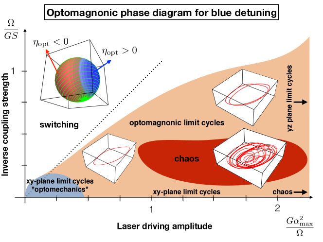
with $c(t)$ given by Eq. (3.3.1). The nonlinear dynamics in this case reduces to the one known for optomechanical systems in the classical limit [72]. Fig. (3.3.1) presents a qualitative, schematic phase diagram for the optomagnonic system in the blue detuned regime as a function of laser power and coupling strength, highlighting the different possible nonlinear regimes.

Chapter 4 Optomagnonics with a magnetic vortex

In this section we come back to the issue of calculating the optomagnonic coupling in the presence of a smooth magnetic textures and structured optical modes, as given by Eq. (2.2.25). By smooth magnetic textures we refer to a magnetization profile that can be represented by a continuous vector field with constant length, given in our case by $\mathbf{M}(\mathbf{r})=M_{{\rm s}}\mathbf{m}(r)$. As an example, we will consider a cavity system with cylindrical geometry. The optical cavity is a dielectric microdisk which can also host magnetic modes. Due to the size and geometry, the magnetic ground state is a vortex. We will calculate explicitly the optomagnonic coupling of whispering gallery modes in the disk, to a magnetic excitation localized at the vortex core. In this section we follow Ref. [44].

4.0.1 Magnetic vortex

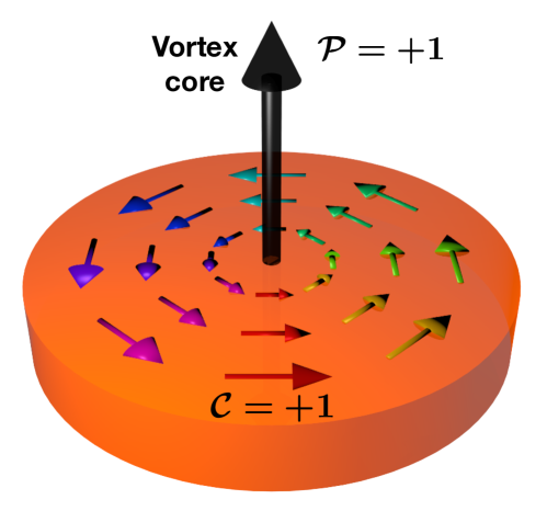
A paradigmatic example of a magnetic texture is a magnetic vortex, which is the stable ground state configuration in magnetic disks with radial dimensions in the $\mu{\rm m}$ range. The vortex forms due to a competition between demagnetizing fields, which tend to align with the surfaces of the disk to avoid the formation of sources of stray fields, and the exchange interaction, which tends to align the spins among themselves. The demagnetizing fields are determined by the magnetostatic Poisson equation and have their origin in the dipolar interactions, and are therefore weak but long ranged. The exchange interaction, whose physical origin is the Coulomb interaction together with the Pauli principle of exclusion, is instead strong but short ranged. The effects of these fields become comparable at the microscale, leading to ordered flux closure configurations that, in the case of a cylindrical geometry, take the form of a vortex. In a thin disk (for heights comparable to the exchange length $l_{{\rm ex}}$) the spins are mostly in-plane and curl around the center of the disk. The core of this vortex is situated at the center of the disk, and it consists of spins pointing out of the plane [73]. Besides being ubiquitous, vortices are interesting since they are topological objects with two independent degrees of freedom, the chirality $\mathcal{C}=\pm 1$ (the spins can curl clockwise or anti-clockwise) and the parity $\mathcal{P}=\pm 1$ , indicating if the spins at the vortex core point up or down, see Fig. (4.0.1). Manipulating these degrees of freedom can give rise to new forms of storing and processing information with magnetic systems [74].

Figure 4.0.1: Magnetic vortex in a microdisk. The spins curl in the plane of the disk and at the core of the vortex point out of the plane. Adapted from Ref. [44].

The vortex in the thin disk can be parametrized as

$$\mathbf{m}(\vec{\rho}) =\mathbf{e}_{\varphi} {\rm for}\,\rho\geq b$$ (4.0.1)

$$=\frac{1}{\rho^{2}+b^{2}}\left(\begin{array}[]{c}-2by\\ 2bx\\ \left(b^{2}-\rho^{2}\right)\end{array}\right) {\rm for}\,\rho\leq b$$ (4.0.5)

where $b$ is an effective core radius (of the order of a few $l_{{\rm ex}}$), we have assumed $,\mathcal{C}=\mathcal{P}=1$ and used cylindrical coordinates with origin at the center of the vortex core, $\mathbf{e}_{\varphi}=(\cos\varphi,\sin\varphi,0)$.

The lowest energy magnon mode in this system is a translational mode of the vortex core, which can be shown to be a circular motion. This is due to an effective gyrotropic force proportional to the topological charge of the vortex, which effectively acts on the vortex core as a magnetic field acts on a charged particle [75]. This mode is denominated gyrotropic and is usually in the range of hundreds of ${\rm MHz}$. It gives rise to a time-dependent magnetization that can be approximated as

$$\mathbf{m_{{\rm ex}}}(\mathbf{r},t)=\mathbf{m}(\mathbf{r}-r_{c}(t))\approx\mathbf{m}(\mathbf{r})-\left(r_{c}(t)\cdot\nabla\right)\mathbf{m}(\mathbf{r})\,,$$ (4.0.6)

where $\mathbf{r}_{c}(t)=r_{c}\left[\cos(\omega_{g}t)\mathbf{e}_{x}+\sin(\omega_{g}t)\mathbf{e}_{y}\right]$ parametrizes the time-dependent position of the vortex core measured from its equilibrium position (we have ignored the damping of the mode). Therefore we can write

$$\delta\mathbf{m}(\mathbf{r},t)=-\left(r_{c}(t)\cdot\nabla\right)\mathbf{m}(\mathbf{r})\,.$$ (4.0.7)

From Eqs. (4.0.1) and (4.0.7) one can obtain analytical expressions for the gyrotropic mode profile $\delta\mathbf{m}(\mathbf{r})$. Together with the normalization prescription Eq. (2.2.21) one obtains the profile of the mode normalized to one magnon [44].

4.0.2 Optomagnonic coupling for the gyrotropic mode

We proceed now to calculate an analytical expression for the coupling of the gyrotropic mode to an optical WGM in the 2D limit. In order to obtain a finite coupling, the gyrotropic mode needs to have overlap with the WGM, which lives near the rim of the disk, see Fig. (4.0.2) (a). The core of the vortex can be displaced from the center of the magnetic disk by applying an external in-plane magnetic field, as the spins will try to align with the field. To a first approximation, the position of the disk $s$ varies linearly with magnetic field, although this breaks down as the vortex approaches the rim. We will moreover use the “rigid vortex” approximation, which implies that the vortex moves but does not deform, so that Eqs. (4.0.1) are always valid as a parametrization of the vortex. It is known that this approximation also fails close to the rim of the disk [73]. Our model therefore is valid for thin disks and its accuracy will diminish as the vortex approaches the rim of the disk.

Figure 4.0.2: Gyrotropic magnon mode and WGM mode and their respective coupling. (a) WGM of a micromagnetic disk together with the gyrotropic magnon mode of a displaced magnetic vortex core. The vortex core has been statically displaced by an applied magnetic field $\mathbf{H}_{x}$ along the $x$ direction. (b) Spatial dependence of the optomagnonic coupling, $G(\mathbf{r},\mathbf{H}_{x})$ before integrating over the volume to obtain the to total coupling, $G=\int_{V}{\rm d}^{3}rG(\mathbf{r},\mathbf{H}_{x})$. The results were obtained with finite element simulations for the optics and MuMax3 [76] micromagnetic simulations for the magnetics, for a thin YIG disk. In order to confine the optical WGM, a cylindrical heterostructure consisting of a thin YIG layer between SiN layers was considered, see Ref. [44] for details.

The WGMs in cylindrical geometry, considering as an approximation an infinite cylinder along $z$, so that the results will be independent of $z$ due to translation invariance and effectively two-dimensional, are given by the solution to the Helmholtz equation

$$\left(\nabla^{2}+n^{2}k_{0}^{2}\right)\psi=0,$$ (4.0.8)

where $\psi=E_{z}$ or $\psi=B_{z}$ respectively for the TM ($\mathbf{B}\perp\mathbf{e}_{z}$) and the TE ($\mathbf{E}\perp\mathbf{e}_{z}$) mode, and $n$ is the index of refraction of the confining dielectric (e.g. YIG). In cylindrical coordinates $(r,\theta)$ with origin at the center of the disk, the solutions for $r<R$ ($R$ the radius of the disk) are of the form ($k=nk_{0}$)

$$\psi(r,\theta)=A_{m}J_{m}(kr)e^{i(\pm m\theta)}\,,$$ (4.0.9)

with $J_{m}$ the Bessel function of the first kind together with the boundary condition

$$K\partial_{r}J{}_{m}(nkR)/J_{m}(nkR)=\partial_{r}H^{(1)}{}_{m}(kR)/H_{m}^{(1)}(kR)$$ (4.0.10)

with $H_{m}^{(1)}$ the Hankel function of the first kind and $K=n$ for a TM and $K=1/n$ for a TE mode. One obtains

$$\mathbf{E}_{mp}^{{\rm TM}} =\psi_{mp}(r,\theta)\mathbf{e}_{z}\,,$$ (4.0.11)

$$\mathbf{E}_{mp}^{{\rm TE}} =\frac{i}{\varepsilon\tilde{\omega}_{mp}}\left(\frac{1}{r}\partial_{\theta}\psi_{mp}\mathbf{e}_{r}-\partial_{r}\psi_{mp}\mathbf{e}_{\theta}\right)\,,$$ (4.0.12)

where the tilde indicates that the solutions are complex: $\tilde{\omega}=\frac{c}{n}\,\tilde{k}=\omega+\frac{i\kappa}{2}$, and the subscripts $mp$ indicates that the expressions are evaluated for a particular solution $\tilde{k}=\tilde{k}_{mp}=k_{mp}-ik_{mp}^{\prime\prime}$ of Eq. (4.0.10). In the following we consider only WGMs solutions, which correspond to $p=1$ (one node in the radial direction), hence we will omit this index. Well defined WGMs are solutions with small imaginary part $k_{m1}^{\prime\prime}$, since this is related to the leaking of the optical mode out of the cavity. The imaginary part gives the decay rate of the mode due to coupling to external unbounded optical modes, and will enter in the total decay rate of the mode. The normalization of the WGM can found by imposing Eq. (2.2.9).

We consider for simplicity the optomagnonic coupling to only one WGM. One can easily show that the only possibility for finite coupling in the 2D limit is to couple to the TE mode [44]. It is straightforward to obtain

$$G_{m}\!=\!-i\frac{\theta_{{\rm F}}\lambda_{n}}{4\pi}\frac{\varepsilon_{0}\varepsilon}{2}h\!\int_{0}^{b}\!\!\rho d\rho\int_{0}^{2\pi}\!\!d\varphi m_{z}(\rho,\varphi)\left(\mathbf{E}_{m}^{{\rm TE}*}\times\mathbf{E}_{m}^{{\rm TE}}\right)\cdot\mathbf{e}_{z}$$ (4.0.13)

where $(\rho,\varphi)$ are polar coordinates in the system with origin at the center of the vortex (note that the center of the vortex can be displaced by an external magnetic field, see Fig. (4.0.2)). From Eq.(4.0.12) we obtain

$$G_{\pm m}\!=\!\pm\frac{\theta_{{\rm F}}\lambda_{n}}{2\pi}\frac{\hbar\omega_{m}}{2\pi\mathcal{N}_{J}}r_{c}k_{m}m\int_{0}^{1}d\rho\int_{0}^{2\pi}d\varphi e^{i\varphi}\frac{\rho^{2}}{\left(\rho^{2}+1\right)^{2}}\frac{\partial_{\tilde{r}}|J_{m}(\tilde{r})|^{2}}{|\left(s/b\right)\mathbf{e}_{y}+\rho\mathbf{e}_{\rho}|}\,,$$ (4.0.14)

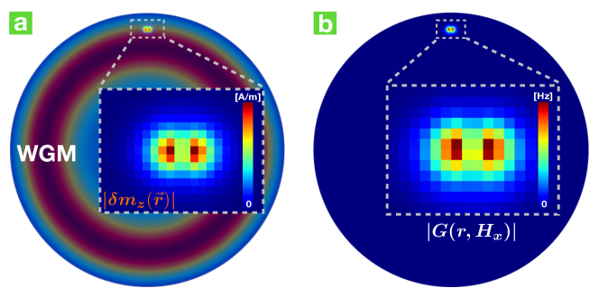
with $\tilde{r}=k_{m}r$, $\mathbf{r}=s\mathbf{e}_{y}+\rho\mathbf{e}_{\rho}$, and $\omega_{m}=\frac{c}{n}k_{m}$. $r_{c}$ and $\mathcal{N}_{J}$ are the corresponding normalization factors for the magnon and optical modes and depend on the geometrical parameters of the system. An example of the spatial structure of the coupling (4.0.14) is shown in Fig. (4.0.2) (b), where the results were obtained via micromagnetics [76] and finite element simulations for the optics. One can show that the first order contribution to Eq. (4.0.14) is proportional to the gradient of the optical spin density with respect to the vortex position. This can be also seen in the results of Fig. (4.0.3).

Figure 4.0.3: Optomagnonic coupling (red) as a function of the vortex position according to Eq. (4.0.14). Also shown is the (normalized) magnitude of the optical spin density (see Eq. (2.2.3)) at the position of the vortex. From the plot it is evident that the coupling is proportional to the gradient of the optical spin density. The inset shows the magnetic vortex at zero field and at an arbitrary finite magnetic field along $x$. Radius of the YIG thin disk $R=1\mu{\rm m}$), WGM with $m=6$, $\omega_{{\rm opt}}/2\pi\approx 200{\rm THz}$. Adapted from Ref. [44].

The 2D approximation works quite well for a thin YIG disk, as we have shown in Ref. [44], where we compared the analytical results with results obtained by combining micromagnetic and finite element simulations. Whereas the thin disk is perfectly fine to host the magnon modes, it is a bad optical cavity since it is not able to confine the light. As a rule of thumb, the thickness of the dielectric has to be of the order of at least half of the wavelength of the light in the material in order to confine it effectively. For this reason, we proposed a “sandwich” heterostructure, where the YIG thin disk is sandwiched between thicker layers of SiN which serve to confine the light. The index of refraction of the transparent dielectric SiN is similar to that of YIG in the optical range, so it is a good choice of material. This however has the effect of decreasing the magnon-to-optical volume ratio, which is detrimental for the optomagnonic coupling as discussed previously. A solution to enhance the coupling was proposed in Ref. [44], where instead of a thin disk a thicker YIG structure was considered. In this case however, the 2D approximation breaks down and the results for the coupling necessarily must be obtained numerically. Promising high values for the coupling and cooperativity were obtained, indicating the value of studying and designing optomagnonic systems beyond the homogeneous, Kittel mode case.

Chapter 5 A quantum protocol: all-optical magnon heralding

To finish this chapter, we study a possible quantum protocol in a cavity optomagnonic system, as proposed in Ref. [77]. In the protocol, a one-magnon Fock state is created in the magnetic material by the detection of a photon. This is referred to as heralding, since the detected photon announces the creation of the desired state. A Fock state, also called a number state since it has a well-defined occupation number, is a purely nonclassical state (as compared for example with a coherent state) characterized by a negative Wigner function. A magnon Fock state is, therefore, a macroscopic collective (involving millions of spins) nonclassical state of the magnetic system, and its realization can be the first step towards the generation, manipulation, and transfer of quantum states in optomagnonic systems [35, 39]. Our protocol proposal includes generating the magnon Fock state optically and reading the state, also optically, at some time later. Due to the optomagnonic interaction, photons and magnons are entangled during the evolution, and detecting a photon projects the magnon sate. The successful generation of the nonclassical state is tested by measuring the two-photon correlations of a “reading” laser. We consider a system with two optical modes and one relevant magnon mode, in line with current experimental setups involving optical whispering gallery modes in YIG spheres [24, 25, 26].

5.1 Hamiltonian and Langevin Equations of Motion

In this section, we analyze the quantum Langevin equations of motion of the cavity optomagnonic system in the spin-wave regime for a system with two non-degenerate optical modes $\hat{a}_{1}$ and $\hat{a}_{2}$ interacting with one magnon mode $\hat{m}$. We will find the analytical solutions for the evolution of the quantum fields by linearizing also in the optical fields, as in Eq. (2.2.19). Our analysis is valid for any magnetization texture and magnon mode (including the homogeneous case), but it is restricted to small oscillations of the spins.

In this case the Hamiltonian in Eq. (2.3.9) reduces to

$$\hat{H} = -\hbar\Delta_{1}\hat{a}_{1}^{\dagger}\hat{a}_{1}-\hbar\Delta_{2}\hat{a}_{2}^{\dagger}\hat{a}_{2}$$

$$+ {\displaystyle\hbar\Omega\hat{m}^{\dagger}\hat{m}+\hbar}\left(G_{12}\hat{a}_{1}^{\dagger}\hat{a}_{2}+G_{21}\hat{a}_{2}^{\dagger}\hat{a}_{1}\right)\hat{m}^{\dagger}+h.c.$$

$$+ i\sum_{j}\epsilon_{j}(\hat{a}_{j}^{\dagger}-\hat{a}_{j})\,,$$ (5.1.2)

where we consider that modes $j=1,\,2$ are driven at frequency $\omega_{{\rm L}}$ and amplitude $\epsilon_{j}$ given by Eq. (2.3.6), and $\Delta_{j}=\omega_{L}-\omega_{j}$ is the respective detuning. The particularity of the cavity optomagnonic system involving spherical WGMs is the asymmetry between the scattering rates $G_{12}$ and $G_{21}$, due to energy and angular momentum conservation rules [26]. In particular, one of the two processes is highly suppressed, which we reflect by setting

$$G_{21}=0=G_{21}^{*}$$ (5.1.3)

in Eq. (5.1). Accordingly, we consider two optical modes satisfying approximately the resonance condition $\omega_{2}-\omega_{1}\approx\Omega$. Applying Eq. (3.1.1) to each of the field operators, and including dissipative and noise terms both for photons and magnons following Eq. (3.2.12), we obtain

$$\frac{d\hat{a}_{1}}{dt} = i\Delta_{1}\hat{a}_{1}-iG_{12}{\displaystyle\hat{a}_{2}}\hat{m}^{\dagger}-\frac{\kappa}{2}\hat{a}_{1}+\sqrt{\kappa}\,\hat{a}_{{\rm 1,in}}(t)+\epsilon_{1}\,,$$ (5.1.4)

$$\frac{d\hat{a}_{2}}{dt} = i\Delta_{2}\hat{a}_{2}-iG_{12}^{*}{\displaystyle\hat{a}_{1}}\hat{m}-\frac{\kappa}{2}\hat{a}_{2}+\sqrt{\kappa}\,\hat{a}_{{\rm 2,in}}(t)+\epsilon_{2}\,,$$

$$\frac{d\hat{m}}{dt} = -i\Omega\hat{m}-iG_{12}\hat{a}_{1}^{\dagger}\hat{a}_{2}-\frac{\Gamma}{2}\hat{m}++\sqrt{\Gamma}\hat{m}_{{\rm in}}(t)\,,$$

where we have assumed for simplicity that both photon modes are subject to the same decay rate $\kappa$. Whereas the photon bath can be considered to be at zero temperature due to the high frequency of the optical photons,

$$\langle\hat{a}_{i,{\rm in}}(t)\hat{a}_{j,{\rm in}}^{\dagger}(t^{\prime})\rangle =\delta_{ij}\delta(t-t^{\prime})\,,$$ (5.1.5)

$$\langle\hat{a}_{i,{\rm in}}^{\dagger}(t)\hat{a}_{j,{\rm in}}(t)\rangle =0\,,$$

the magnons have usually ${\rm GHz}$ frequencies and the temperature of the thermal bath cannot be ignored, unless the system is cooled to mK temperatures. The general expressions for the magnon correlators are

$$\langle\hat{m}_{{\rm in}}(t)\hat{m}_{{\rm in}}^{\dagger}(t^{\prime})\rangle = (n_{{\rm tm}}+1)\delta(t-t^{\prime}),$$ (5.1.6)

$$\langle\hat{m}_{{\rm in}}^{\dagger}(t)\hat{m}_{{\rm in}}(t^{\prime})\rangle = n_{{\rm{\rm tm}}}\delta(t-t^{\prime})\,,$$ (5.1.7)

where the subscript ${\rm tm}$ indicates that $n_{{\rm{\rm tm}}}$ is the mean number of thermal magnons given by the Bose-Einstein distribution

$$n_{{\rm{\rm tm}}}(T)=\frac{1}{\exp\left(\hbar\,\Omega/k_{B}T\right)-1}\,,$$ (5.1.8)

where $T$ is the temperature of the magnon bath and $k_{B}$ the Boltzmann constant, and $\Omega$ is the magnon mode frequency.

The steady state values $\langle\hat{a}_{i}\rangle=\alpha_{i}$ and $\langle\hat{m}\rangle=\beta$ are found by setting Eqs. (5.1.4) to zero and ignoring the noise fluctuations. The expectation values of the operators are understood to be taken with respect to a coherent state. In the side-band resolved limit ( $\Omega\gg\kappa,\gamma$ ) it is straightforward to see that if only one mode $j$ (=1 or 2) is driven, $\beta=0$ and the steady state circulating number of photons in the cavity is given by $|\alpha_{j}|^{2}$ with

$$\alpha_{j}=-\frac{\epsilon_{j}}{i\Delta_{j}-\kappa_{j}/2}.$$ (5.1.9)

By considering the fluctuations around the steady state $\hat{a}_{i}\rightarrow\alpha_{i}+\hat{a}_{i}$, $\hat{m}\rightarrow\hat{m}$ (where for simplicity of notation we denote now the fluctuations by $\hat{a}_{i}$ and $\hat{m}$) one obtains the Hamiltonian valid in the linear regime, as in Eq. (2.3.11). In the interaction picture the resulting Hamiltonian reads

$$\hat{H}_{{\rm IP}} \approx\hbar\alpha_{1}^{*}G_{12}\hat{a}_{2}\hat{m}^{\dagger}e^{i(\Delta_{2}+\Omega)t}+\hbar\alpha_{2}G_{12}\hat{a}_{1}^{\dagger}\hat{m}^{\dagger}e^{-i(\Delta_{1}-\Omega)t}+h.c.\,.$$ (5.1.10)

5.2 Write and read protocol

From Eq. (5.1.10) one can immediately observe that by pumping the optical mode 2 at resonance ($\omega_{{\rm L}}=\omega_{2}\approx\omega_{1}+\Omega$) while mode 1 is not driven ($\alpha_{1}=0$), the condition $\Delta_{1}=\Omega$ is satisfied and one obtains

$$\hat{H}_{{\rm{\rm W}}}\approx\hbar\left[\alpha_{2}^{*}G_{12}^{*}\hat{a}_{1}\hat{m}+\alpha_{2}G_{12}\hat{a}_{1}^{\dagger}\hat{m}^{\dagger}\right]\,,$$ (5.2.1)

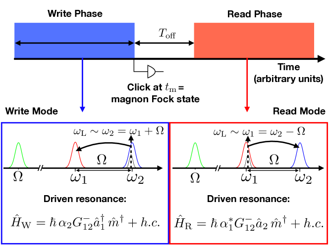
in which a magnon and a photon in mode 1 are either created or annihilated in pairs. We denote this effective Hamiltonian as $\hat{H}_{{\rm{\rm W}}}$ since it corresponds to the writing Hamiltonian is our protocol. Starting from the vacuum of magnons and photons, the evolution under this Hamiltonian creates entangled pairs of magnons and mode-1 photons. Detecting a photon in mode 1 collapses the entangled state and determines the magnon state, with a certain probability of collapsing into a one-magnon Fock state [77]. The Fock state created in this form is denominated heralded.

The successful heralding of a magnon Fock state can be corroborated by a reading protocol, as long this is done within the lifetime of the state, that is , the lifetime of the magnon. The reading Hamiltonian is obtained from Eq. (5.1.10) by this time driving the optical mode 1 at resonance ($\omega_{{\rm L}}=\omega_{1}\approx\omega_{2}-\Omega$) and not driving mode 2 ($\alpha_{2}=0$). One obtains

$$\hat{H}_{{\rm{\rm R}}}\approx\hbar\left[\alpha_{1}^{*}G_{12}\hat{a}_{2}\hat{m}^{\dagger}+\alpha_{1}G_{12}^{*}\hat{a}_{2}^{\dagger}\hat{m}\right]\,.$$ (5.2.2)

In the strong coupling regime, such that the effective coupling strength $G_{1,12}^{{\rm eff}}=|\alpha_{1}G_{12}|$ is larger than the decay channels $|\alpha_{1}G_{12}|>\kappa,\,\Gamma$, the magnon mode and the photon mode hybridize, giving rise to eigenmodes which are part magnon, part photon, in analogy with the cavity magnon polariton discussed previously in the MW regime. Moreover, if $|\alpha_{1}G_{12}|>\kappa,\,n_{{\rm tm}}\Gamma$ (denominated the coherent coupling regime) the interaction is quantum-coherent, allowing to transfer the magnon state coherently to the photons. Therefore measuring the mode-2 photons give information on the magnon state, that is, we can “read” the state. The write-and-read protocol is described schematically in Fig. (5.2.1).

Figure 5.2.1: Write and read protocol for heralding a magnon Fock state. The detection of a photon at time $t_{{\rm m}}$ is a probabilistic process. Figure taken from Ref. [77].

As we pointed out in the introduction, the strong coupling regime in optomagnonics is challenging to attain and experiments have not yet reached this point. Nevertheless, photons in mode 2 can be used to probe the heralded state even in the weak coupling regime. This can be done by measuring the two-photon correlation function [68]

$$g_{{\rm Read}}^{(2)}(t,t+\tau)=\frac{\langle\hat{a}_{2}^{\dagger}(t)\hat{a}_{2}^{\dagger}(t+\tau)\hat{a}_{2}(t+\tau)\hat{a}_{2}(t)\rangle}{\langle\hat{a}_{2}^{\dagger}(t)\hat{a}_{2}(t)\rangle\langle\hat{a}_{2}^{\dagger}(t+\tau)\hat{a}_{2}(t+\tau)\rangle}\,,$$ (5.2.3)

which can be done interferometrically. In order to use this quantity as a heralding witness, the expectation values have to be taken after the measurement of a “write” photon (a mode-1 photon). Given the form of the read Hamiltonian from Eq. (5.2.2), which “swaps” magnons with photons, measuring $g_{{\rm Read}}^{(2)}$ for the photons is equivalent to measure the corresponding correlation function for the magnons. If the state is non-classical, $g_{{\rm Read}}^{(2)}(t,t)<1$, given an indication that the heralded magnon state is a Fock state. The condition $g_{{\rm Read}}^{(2)}(t,t)<1$ is denominated antibunching, since there is a reduced probability of two photons being detected simultaneously, and it is an example of a quantum state violating a classical inequality ($g_{{\rm Read}}^{(2)}(t,t)>1$ necessarily for classical states). The reliability of $g_{{\rm Read}}^{(2)}$ as a true heralding witness depends however on the temperature of the magnon bath, worsening as the temperature and consequently the number of thermal magnons increases [77].

5.3 Solution of the linear quantum Langevin equations

The probability of heralding a magnon, as well as the correlation function $g_{{\rm Read}}^{(2)}$, can be calculated by the linear quantum Langevin equations dictated by the Hamiltonians of Eq. (5.2.1) and (5.2.2) with the steady state given by Eqs. (5.1.4) and using the noise correlators of Eqs. (5.1.5) and (5.1.6). The linear Langevin equations can be written in compact form as

$$\frac{d\hat{\bm{A}}}{dt}=M^{{\rm X}}\cdot\hat{\bm{A}}(t)+\bm{\hat{N}}(t),$$ (5.3.1)

where

$$\hat{\bm{A}}=\left(\begin{array}[]{c}\hat{a}_{1}^{\dagger}\\ \hat{m}\\ \hat{a}_{2}\end{array}\right), \hat{\bm{N}}=\left(\begin{array}[]{c}\sqrt{\kappa}(\hat{a}_{1}^{in})^{\dagger}\\ \sqrt{\gamma}\hat{m}^{in}\\ \sqrt{\kappa}\hat{a}_{2}^{in}\end{array}\right),$$ (5.3.8)

${\rm X}={\rm W},$ ${\rm R}$ indicates the write or read phases of the protocol, and $M^{{\rm X}}$ is a matrix given by the Heisenberg equation of motion deriving from Hamiltonians (5.2.1) or (5.2.2) . The solution can be written formally as

$$\hat{\bm{A}}(t)=U^{{\rm X}}(t)\cdot\hat{\bm{A}}(0)+{\displaystyle\int}_{0}^{t}d\tau U^{{\rm X}}(t-\tau)\cdot\hat{\bm{N}}(\tau),$$ (5.3.9)

where $U^{{\rm W}}(t)$ and $U^{{\rm R}}(t)$ are the respective evolution matrices. These can be found analytically by going to a diagonal basis such that

$$\frac{d\hat{A}_{i}^{\prime}}{dt}=\lambda_{i}^{{\rm P}}\hat{A}_{i}^{\prime}(t)+\hat{N}_{i}^{\prime}(t),$$ (5.3.10)

which can be easily integrated and transformed back to find $U^{{\rm W}}(t)$ and $U^{{\rm R}}(t)$. The expressions for $U^{{\rm W}}(t)$ and $U^{{\rm R}}(t)$ are lengthy and can be found in Ref. [77].

5.4 Probability of heralding a magnon

The probability of heralding a magnon is given by the probability of detecting a photon in mode 1 during the write phase. This is given by (see e.g. Ref. [68])

$$P_{1,{\rm W}}(t)=\langle:\hat{a}_{1}^{\dagger}\hat{a}_{1}\exp(-\hat{a}_{1}^{\dagger}\hat{a}_{1}):\rangle\sim\langle\hat{a}_{1}^{\dagger}\hat{a}_{1}\rangle-\langle\hat{a}_{1}^{\dagger}\hat{a}_{1}^{\dagger}\hat{a}_{1}\hat{a}_{1}\rangle\,,$$

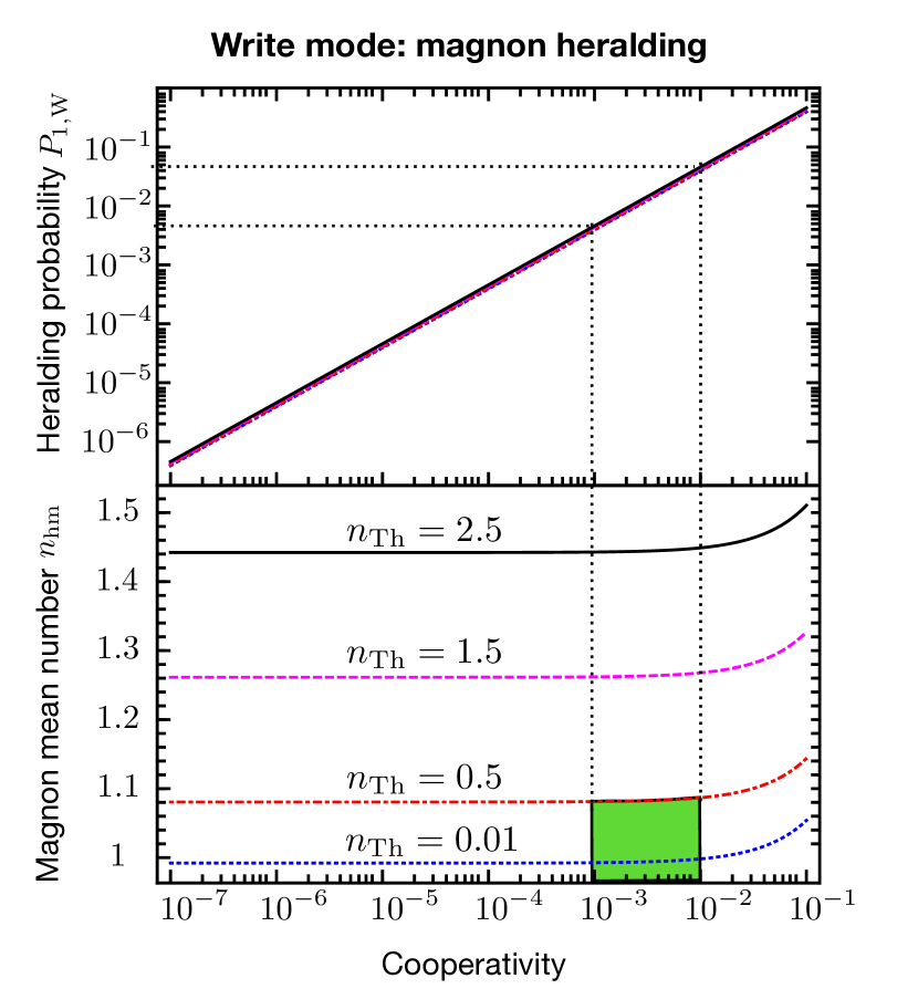
where the approximation is valid as long as $\langle\hat{a}_{1}^{\dagger}\hat{a}_{1}^{\dagger}\hat{a}_{1}^{\dagger}\hat{a}_{1}\hat{a}_{1}\hat{a}_{1}\rangle\ll\langle\hat{a}_{1}^{\dagger}\hat{a}_{1}^{\dagger}\hat{a}_{1}\hat{a}_{1}\rangle$. This probability can be computed by the method outlined previously, on the basis of the solution for the equations of motion (5.3.1) for the write-Hamiltonian. One finds that the heralding probability grows linearly with the square of the effective optomagnonic coupling during the write phase. A very large coupling is however detrimental, since it will tend to generate a larger number of magnons within the same period, compromising the Fock state. Therefore an optimal effective coupling strength $G_{1,12}^{{\rm eff}}$ must be found, see Fig. (5.4.1). The mean number of magnons $n_{{\rm hm}}=\langle\hat{m}^{\dagger}\hat{m}\rangle$ after the heralding event depends crucially on the temperature of the magnon bath, as shown in Fig. (5.4.1).

Figure 5.4.1: Probability of heralding a magnon and mean number of heralded magnons as a function of the write cooperativity, $\mathcal{C}=4G_{1,12}^{{\rm eff}}/\kappa\Gamma$. The shaded area indicates values of the cooperativity which give an appreciable heralding probability while keeping the number of heralded magnons near one. The number of thermal magnons $n_{{\rm tm}}$ is dictated by the temperature of the magnon bath, larger temperatures are, as expected, detrimental for the heralding protocol. Figure taken from Ref. [77].

5.5 Magnon cooling

As we have seen in the heralding example, the presence of thermal magnons is highly detrimental for quantum protocols. Due to their larger frequencies (usually in the ${\rm GHz}$ range in optomagnonic setups), magnons are generally more amenable to direct cooling than, for example, phonons in optomechanical systems. However light can be used for active cooling in cases in which direct cooling is not sufficient or inconvenient from and experimental point of view. Magnon cooling in optomagnonic systems has been studied in detail in Ref. [78].

The formalism described to solve the quantum Langevin equations of motion can be used to study the cooling protocol exactly, including all decay channels and quantum fluctuations. In particular, our “read” Hamiltonian can be used for magnon cooling, since it effectively annihilates magnons when mode 1 is driven. If we consider an initial thermal state state with a mean number of magnons $n_{{\rm th}}$, the initial density matrix of the optomagnonic system is given by

$$\rho(0) = |0\rangle\langle 0|_{1}\otimes|0\rangle\langle 0|_{2}\otimes\rho_{{\rm th,m}},$$ (5.5.1)

where

$$\rho_{{\rm th,\,m}}=\frac{1}{1+n_{{\rm th}}}\sum_{n\geq 0}\left[\frac{n_{{\rm th}}}{1+n_{{\rm th}}}\right]^{n}|n\rangle\langle n|,$$ (5.5.2)

indicates that the initial population of magnons os a thermal state. The temporal evolution of the mean number of magnons is given by

$$\langle\hat{m}^{\dagger}\hat{m}\rangle(t) =\sum_{i,j} \left(U_{i2}^{{\rm R}}(t)\right)^{*}U_{2j}^{{\rm R}}(t)\langle\hat{A}_{i}^{\dagger}(0)\hat{A}_{j}(0)\rangle$$

$$+ \sum_{i,j}{\displaystyle\int}_{0}^{\,t}d\tau_{1}d\tau_{2}\left(U_{i2}^{{\rm R}}(t-\tau_{1})\right)^{*}U_{2j}^{{\rm R}}(t-\tau_{2})\langle\hat{N}_{i}^{\dagger}(\tau_{1})\hat{N}_{j}(\tau_{2})\rangle\,,$$

where $i,j$ indicate the components of $\hat{\mathbf{A}}$, $\hat{\mathbf{N}}$, and $U^{{\rm R}}$ as defined in Eqs. (5.3.8) and (5.3.9), and the expectation values are taken over the initial state determined by $\rho(0)$. Imposing the noise correlators of Eqs. (5.1.5) and (5.1.6) one obtains

$$\langle\hat{m}^{\dagger}\hat{m}\rangle(t) = |U_{22}^{{\rm R}}(t)|^{2}n_{{\rm th}}+|U_{12}^{{\rm R}}(t)|^{2}$$

$$+ \int_{0}^{t}d\tau\left[|U_{12}^{{\rm R}}(t-\tau)|^{2}+|U_{22}^{{\rm R}}(t-\tau)|^{2}n_{{\rm th}}\right].$$

The steady state value $n_{0}=\langle\hat{m}^{\dagger}\hat{m}\rangle(t\rightarrow\infty)$ can be shown to be

$$n_{0}=\frac{\Gamma n_{{\rm th}}}{(\kappa+\Gamma)}\left(1+\frac{\kappa}{\Gamma(1+C_{{\rm R}})}\right),$$

where $C_{{\rm R}}=4|\alpha_{1}^{*}G_{1{\rm 2}}|^{2}/\kappa\Gamma$ is the read-phase cooperativity. This is a thermal state with $n_{0}<n_{{\rm th}}$, and therefore it is cooled. Whereas active cooling is necessary for most implementations of optomechanical systems, given that phonon frequencies are usually low, for optomagnonic systems this can be circumvented by cooling the system by usual dilution fridge refrigeration techniques.

Chapter 6 Outlook

Cavity optomagnonic systems are at the interface between condensed matter and quantum optics, and present new opportunities to study and control the interaction between light and magnetic systems, in particular at the single quanta level. Magnons are robust elementary excitations, highly tunable and can couple well to several other degrees of freedom beyond photons, such as phonons and electrons. The incorporation of magnetically ordered systems into hybrid platforms for quantum information is therefore very promising. From a fundamental point of view, cavity optomagnonic systems are very rich. Topics such as the interaction of structured light with magnetic textures and topological defects, the nonlinear dynamics of the coupled system, or collective quantum effects in cavity optomagnonics taking into account the strongly correlated nature of the magnetically ordered systems, are still largely unexplored. There are exciting times ahead for theorists and experimentalists alike.

References

- [1] A. G. J. MacFarlane, Jonathan P. Dowling, and Gerard J. Milburn. Quantum technology: The second quantum revolution. Philosophical Transactions of the Royal Society of London. Series A: Mathematical, Physical and Engineering Sciences, 361(1809):1655–1674, August 2003.
- [2] Frank Arute, Kunal Arya, Ryan Babbush, Dave Bacon, Joseph C. Bardin, Rami Barends, Rupak Biswas, Sergio Boixo, Fernando G. S. L. Brandao, David A. Buell, Brian Burkett, Yu Chen, Zijun Chen, Ben Chiaro, Roberto Collins, William Courtney, Andrew Dunsworth, Edward Farhi, Brooks Foxen, Austin Fowler, Craig Gidney, Marissa Giustina, Rob Graff, Keith Guerin, Steve Habegger, Matthew P. Harrigan, Michael J. Hartmann, Alan Ho, Markus Hoffmann, Trent Huang, Travis S. Humble, Sergei V. Isakov, Evan Jeffrey, Zhang Jiang, Dvir Kafri, Kostyantyn Kechedzhi, Julian Kelly, Paul V. Klimov, Sergey Knysh, Alexander Korotkov, Fedor Kostritsa, David Landhuis, Mike Lindmark, Erik Lucero, Dmitry Lyakh, Salvatore Mandrà, Jarrod R. McClean, Matthew McEwen, Anthony Megrant, Xiao Mi, Kristel Michielsen, Masoud Mohseni, Josh Mutus, Ofer Naaman, Matthew Neeley, Charles Neill, Murphy Yuezhen Niu, Eric Ostby, Andre Petukhov, John C. Platt, Chris Quintana, Eleanor G. Rieffel, Pedram Roushan, Nicholas C. Rubin, Daniel Sank, Kevin J. Satzinger, Vadim Smelyanskiy, Kevin J. Sung, Matthew D. Trevithick, Amit Vainsencher, Benjamin Villalonga, Theodore White, Z. Jamie Yao, Ping Yeh, Adam Zalcman, Hartmut Neven, and John M. Martinis. Quantum supremacy using a programmable superconducting processor. Nature, 574(7779):505–510, October 2019.
- [3] H. J. Kimble. The quantum internet. Nature, 453:1023–1030, June 2008.
- [4] A. D. O’Connell, M. Hofheinz, M. Ansmann, Radoslaw C. Bialczak, M. Lenander, Erik Lucero, M. Neeley, D. Sank, H. Wang, M. Weides, J. Wenner, John M. Martinis, and A. N. Cleland. Quantum ground state and single-phonon control of a mechanical resonator. Nature, 464(7289):697–703, April 2010.
- [5] Jasper Chan, T. P. Mayer Alegre, Amir H. Safavi-Naeini, Jeff T. Hill, Alex Krause, Simon Gröblacher, Markus Aspelmeyer, and Oskar Painter. Laser cooling of a nanomechanical oscillator into its quantum ground state. Nature, 478(7367):89–92, October 2011.
- [6] J. D. Teufel, T. Donner, Dale Li, J. W. Harlow, M. S. Allman, K. Cicak, A. J. Sirois, J. D. Whittaker, K. W. Lehnert, and R. W. Simmonds. Sideband cooling of micromechanical motion to the quantum ground state. Nature, 475(7356):359–363, July 2011.
- [7] Markus Aspelmeyer, Tobias J. Kippenberg, and Florian Marquardt. Cavity optomechanics. Rev. Mod. Phys., 86(4):1391–1452, December 2014.
- [8] Ralf Riedinger, Andreas Wallucks, Igor Marinković, Clemens Löschnauer, Markus Aspelmeyer, Sungkun Hong, and Simon Gröblacher. Remote quantum entanglement between two micromechanical oscillators. Nature, 556(7702):473–477, April 2018.
- [9] Gershon Kurizki, Patrice Bertet, Yuimaru Kubo, Klaus Mølmer, David Petrosyan, Peter Rabl, and Jörg Schmiedmayer. Quantum technologies with hybrid systems. PNAS, 112(13):3866–3873, March 2015.
- [10] M. H. Devoret and R. J. Schoelkopf. Superconducting Circuits for Quantum Information: An Outlook. Science, 339(6124):1169–1174, March 2013.
- [11] Mikael Afzelius, Nicolas Gisin, and Hugues de Riedmatten. Quantum memory for photons. Physics Today, 68(12):42–47, November 2015.
- [12] Fabio Pulizzi. Spintronics. Nature Mater, 11(5):367–367, May 2012.
- [13] J. C. Slonczewski. Current-driven excitation of magnetic multilayers. Journal of Magnetism and Magnetic Materials, 159(1):L1–L7, June 1996.
- [14] Sabpreet Bhatti, Rachid Sbiaa, Atsufumi Hirohata, Hideo Ohno, Shunsuke Fukami, and S. N. Piramanayagam. Spintronics based random access memory: A review. Materials Today, 20(9):530–548, November 2017.
- [15] Joseph E. Losby and Mark R. Freeman. Spin Mechanics. arXiv:1601.00674 [cond-mat], January 2016.
- [16] Marcelo Wu, Nathanael L.-Y. Wu, Tayyaba Firdous, Fatemeh Fani Sani, Joseph E. Losby, Mark R. Freeman, and Paul E. Barclay. Nanocavity optomechanical torque magnetometry and radiofrequency susceptometry. Nature Nanotechnology, 12(2):127–131, February 2017.
- [17] Dany Lachance-Quirion, Yutaka Tabuchi, Arnaud Gloppe, Koji Usami, and Yasunobu Nakamura. Hybrid quantum systems based on magnonics. Appl. Phys. Express, 12(7):070101, June 2019.
- [18] Hans Huebl, Christoph W. Zollitsch, Johannes Lotze, Fredrik Hocke, Moritz Greifenstein, Achim Marx, Rudolf Gross, and Sebastian T. B. Goennenwein. High Cooperativity in Coupled Microwave Resonator Ferrimagnetic Insulator Hybrids. Phys. Rev. Lett., 111(12):127003, September 2013.
- [19] Yutaka Tabuchi, Seiichiro Ishino, Toyofumi Ishikawa, Rekishu Yamazaki, Koji Usami, and Yasunobu Nakamura. Hybridizing Ferromagnetic Magnons and Microwave Photons in the Quantum Limit. Phys. Rev. Lett., 113(8):083603, August 2014.
- [20] Xufeng Zhang, Chang-Ling Zou, Liang Jiang, and Hong X. Tang. Strongly Coupled Magnons and Cavity Microwave Photons. Phys. Rev. Lett., 113(15):156401, October 2014.
- [21] J. A. Haigh, N. J. Lambert, A. C. Doherty, and A. J. Ferguson. Dispersive readout of ferromagnetic resonance for strongly coupled magnons and microwave photons. Phys. Rev. B, 91(10):104410, March 2015.
- [22] Ö. O. Soykal and M. E. Flatté. Strong Field Interactions between a Nanomagnet and a Photonic Cavity. Phys. Rev. Lett., 104(7):077202, February 2010.
- [23] Yutaka Tabuchi, Seiichiro Ishino, Atsushi Noguchi, Toyofumi Ishikawa, Rekishu Yamazaki, Koji Usami, and Yasunobu Nakamura. Coherent coupling between a ferromagnetic magnon and a superconducting qubit. Science, 349(6246):405–408, July 2015.
- [24] J. A. Haigh, A. Nunnenkamp, A. J. Ramsay, and A. J. Ferguson. Triple-Resonant Brillouin Light Scattering in Magneto-Optical Cavities. Physical Review Letters, 117(13), September 2016.
- [25] Xufeng Zhang, Na Zhu, Chang-Ling Zou, and Hong X. Tang. Optomagnonic Whispering Gallery Microresonators. Physical Review Letters, 117(12), September 2016.
- [26] A. Osada, R. Hisatomi, A. Noguchi, Y. Tabuchi, R. Yamazaki, K. Usami, M. Sadgrove, R. Yalla, M. Nomura, and Y. Nakamura. Cavity Optomagnonics with Spin-Orbit Coupled Photons. Phys. Rev. Lett., 116(22):223601, June 2016.
- [27] Silvia Viola Kusminskiy, Hong X. Tang, and Florian Marquardt. Coupled spin-light dynamics in cavity optomagnonics. Phys. Rev. A, 94:033821, 2016.
- [28] Tianyu Liu, Xufeng Zhang, Hong X. Tang, and Michael E. Flatté. Optomagnonics in magnetic solids. Phys. Rev. B, 94(6):060405, August 2016.
- [29] Yi-Pu Wang, Guo-Qiang Zhang, Dengke Zhang, Tie-Fu Li, C.-M. Hu, and J. Q. You. Bistability of Cavity Magnon Polaritons. Phys. Rev. Lett., 120(5):057202, January 2018.
- [30] H. Maier-Flaig, M. Harder, S. Klingler, Z. Qiu, E. Saitoh, M. Weiler, S. Geprägs, R. Gross, S. T. B. Goennenwein, and H. Huebl. Tunable magnon-photon coupling in a compensating ferrimagnet—from weak to strong coupling. Appl. Phys. Lett., 110(13):132401, March 2017.
- [31] R. G. E. Morris, A. F. van Loo, S. Kosen, and A. D. Karenowska. Strong coupling of magnons in a YIG sphere to photons in a planar superconducting resonator in the quantum limit. Sci Rep, 7(1):1–6, September 2017.
- [32] Isabella Boventer, Christine Dörflinger, Tim Wolz, Rair Macêdo, Romain Lebrun, Mathias Kläui, and Martin Weides. Control of the Coupling Strength and the Linewidth of a Cavity-Magnon Polariton. arXiv:1904.00393 [cond-mat], March 2019.
- [33] Yi-Pu Wang, Guo-Qiang Zhang, Da Xu, Tie-Fu Li, Shi-Yao Zhu, J. S. Tsai, and J. Q. You. Quantum Simulation of the Fermion-Boson Composite Quasi-Particles with a Driven Qubit-Magnon Hybrid Quantum System. arXiv:1903.12498 [cond-mat, physics:quant-ph], March 2019.
- [34] Graeme Flower, Maxim Goryachev, Jeremy Bourhill, and Michael E. Tobar. Experimental implementations of cavity-magnon systems: From ultra strong coupling to applications in precision measurement. New J. Phys., 21(9):095004, September 2019.
- [35] Dany Lachance-Quirion, Yutaka Tabuchi, Seiichiro Ishino, Atsushi Noguchi, Toyofumi Ishikawa, Rekishu Yamazaki, and Yasunobu Nakamura. Resolving quanta of collective spin excitations in a millimeter-sized ferromagnet. Science Advances, 3(7):e1603150, July 2017.
- [36] J. W. Rao, C. H. Yu, Y. T. Zhao, Y. S. Gui, X. L. Fan, D. S. Xue, and C.-M. Hu. Level attraction and level repulsion of magnon coupled with a cavity anti-resonance. New J. Phys., 21(6):065001, June 2019.
- [37] Isabella Boventer, Mathias Kläui, Rair Macêdo, and Martin Weides. Steering between Level Repulsion and Attraction: Beyond Single-Tone Driven Cavity Magnon-Polaritons. arXiv:1908.05439 [cond-mat, physics:quant-ph], August 2019.
- [38] Yi-Pu Wang, J. W. Rao, Y. Yang, Peng-Chao Xu, Y. S. Gui, B. M. Yao, J. Q. You, and C.-M. Hu. Nonreciprocity and Unidirectional Invisibility in Cavity Magnonics. Phys. Rev. Lett., 123(12):127202, September 2019.
- [39] Dany Lachance-Quirion, Samuel Piotr Wolski, Yutaka Tabuchi, Shingo Kono, Koji Usami, and Yasunobu Nakamura. Entanglement-based single-shot detection of a single magnon with a superconducting qubit. arXiv:1910.09096 [cond-mat, physics:quant-ph], October 2019.
- [40] Justin T. Hou and Luqiao Liu. Strong Coupling between Microwave Photons and Nanomagnet Magnons. Phys. Rev. Lett., 123(10):107702, September 2019.
- [41] Yi Li, Tomas Polakovic, Yong-Lei Wang, Jing Xu, Sergi Lendinez, Zhizhi Zhang, Junjia Ding, Trupti Khaire, Hilal Saglam, Ralu Divan, John Pearson, Wai-Kwong Kwok, Zhili Xiao, Valentine Novosad, Axel Hoffmann, and Wei Zhang. Strong Coupling between Magnons and Microwave Photons in On-Chip Ferromagnet-Superconductor Thin-Film Devices. Phys. Rev. Lett., 123(10):107701, September 2019.
- [42] Michael G. Cottam and David J. Lockwood. Light Scattering in Magnetic Solids. Wiley-Interscience, New York, 1 edition edition, August 1986.
- [43] P. A. Pantazopoulos, N. Stefanou, E. Almpanis, and N. Papanikolaou. Photomagnonic nanocavities for strong light–spin-wave interaction. Phys. Rev. B, 96(10):104425, September 2017.
- [44] Jasmin Graf, Hannes Pfeifer, Florian Marquardt, and Silvia Viola Kusminskiy. Cavity optomagnonics with magnetic textures: Coupling a magnetic vortex to light. Phys. Rev. B, 98(24):241406, December 2018.
- [45] Sanchar Sharma, Babak Zare Rameshti, Yaroslav M. Blanter, and Gerrit E. W. Bauer. Optimal mode matching in cavity optomagnonics. Phys. Rev. B, 99(21):214423, June 2019.
- [46] Petros-Andreas Pantazopoulos, Nikolaos Papanikolaou, and Nikolaos Stefanou. Tailoring coupling between light and spin waves with dual photonic–magnonic resonant layered structures. J. Opt., 21(1):015603, December 2018.
- [47] Evangelos Almpanis. Dielectric magnetic microparticles as photomagnonic cavities: Enhancing the modulation of near-infrared light by spin waves. Phys. Rev. B, 97(18):184406, May 2018.
- [48] A. Osada, A. Gloppe, Y. Nakamura, and K. Usami. Orbital angular momentum conservation in Brillouin light scattering within a ferromagnetic sphere. New J. Phys., 20(10):103018, October 2018.
- [49] A. Osada, A. Gloppe, R. Hisatomi, A. Noguchi, R. Yamazaki, M. Nomura, Y. Nakamura, and K. Usami. Brillouin Light Scattering by Magnetic Quasivortices in Cavity Optomagnonics. Phys. Rev. Lett., 120(13):133602, March 2018.
- [50] J. A. Haigh, N. J. Lambert, S. Sharma, Y. M. Blanter, G. E. W. Bauer, and A. J. Ramsay. Selection rules for cavity-enhanced Brillouin light scattering from magnetostatic modes. Phys. Rev. B, 97(21):214423, June 2018.
- [51] Petros Andreas Pantazopoulos, Kosmas L. Tsakmakidis, Evangelos Almpanis, Grigorios P. Zouros, and Nikolaos Stefanou. High-efficiency triple-resonant inelastic light scattering in planar optomagnonic cavities. New J. Phys., 21(9):095001, September 2019.
- [52] R. Hisatomi, A. Noguchi, R. Yamazaki, Y. Nakata, A. Gloppe, Y. Nakamura, and K. Usami. Helicity-changing brillouin light scattering by magnons in a ferromagnetic crystal. Phys. Rev. Lett., 123:207401, Nov 2019.
- [53] Purcell, E. M. Proceedings of the American Physical Society. Physical Review, 69(11-12):674–674, June 1946.
- [54] Serge Haroche and Daniel Kleppner. Cavity Quantum Electrodynamics. Physics Today, 42(1):24–30, January 1989.
- [55] Herbert Walther, Benjamin T. H. Varcoe, Berthold-Georg Englert, and Thomas Becker. Cavity quantum electrodynamics. Rep. Prog. Phys., 69(5):1325–1382, April 2006.
- [56] R. J. Schoelkopf and S. M. Girvin. Wiring up quantum systems. Nature, 451(7179):664–669, February 2008.
- [57] Daniel D. Stancil and Anil Prabhakar. Spin Waves: Theory and Applications. Springer US, 2009.
- [58] L. D. Landau, L. P. Pitaevskii, and E. M. Lifshitz. Electrodynamics of Continuous Media: Volume 8 (Course of Theoretical Physics S). Butterworth-Heinemann, 2nd edition.
- [59] Silvia Viola Kusminiskiy. Quantum Magnetism, Spin Waves, and Optical Cavities. SpringerBriefs in Physics. Springer International Publishing, 2019.
- [60] Markus Garst, Johannes Waizner, and Dirk Grundler. Collective spin excitations of helices and magnetic skyrmions: Review and perspectives of magnonics in non-centrosymmetric magnets. Journal of Physics D: Applied Physics, 50(29):293002, July 2017.
- [61] C. L. Dennis, R. P. Borges, L. D. Buda, U. Ebels, J. F. Gregg, M. Hehn, E. Jouguelet, K. Ounadjela, I. Petej, I. L. Prejbeanu, and M. J. Thornton. The defining length scales of mesomagnetism: A review. J. Phys.: Condens. Matter, 14(49):R1175, 2002.
- [62] Charles Kittel. Physical Theory of Ferromagnetic Domains. Rev. Mod. Phys., 21(4):541–583, October 1949.
- [63] John Heebner, Rohit Grover, and Tarek Ibrahim. Optical Microresonators: Theory, Fabrication, and Applications. Springer Series in Optical Sciences. Springer-Verlag, New York, 2008.
- [64] Markus Aspelmeyer, Tobias J. Kippenberg, and Florian Marquardt, editors. Cavity Optomechanics: Nano- and Micromechanical Resonators Interacting with Light. Quantum Science and Technology. Springer-Verlag, Berlin Heidelberg, 2014.
- [65] Gregory S. MacCabe, Hengjiang Ren, Jie Luo, Justin D. Cohen, Hengyun Zhou, Alp Sipahigil, Mohammad Mirhosseini, and Oskar Painter. Phononic bandgap nano-acoustic cavity with ultralong phonon lifetime. arXiv:1901.04129 [cond-mat, physics:quant-ph], January 2019.
- [66] Sanchar Sharma, Yaroslav M. Blanter, and Gerrit E. W. Bauer. Light scattering by magnons in whispering gallery mode cavities. Phys. Rev. B, 96(9):094412, September 2017.
- [67] J. A. Osborn. Demagnetizing Factors of the General Ellipsoid. Phys. Rev., 67(11-12):351–357, June 1945.
- [68] D. F. Walls and Gerard J. Milburn. Quantum Optics. Springer-Verlag, Berlin Heidelberg, 2 edition, 2008.
- [69] Pierre Meystre and Murray Sargent. Elements of Quantum Optics. Springer-Verlag, Berlin Heidelberg, 4th edition, 2007.
- [70] A. M. Clogston, H. Suhl, L. R. Walker, and P. W. Anderson. Ferromagnetic resonance line width in insulating materials. Journal of Physics and Chemistry of Solids, 1(3):129–136, November 1956.
- [71] Jonathan Kohler, Nicolas Spethmann, Sydney Schreppler, and Dan M. Stamper-Kurn. Cavity-Assisted Measurement and Coherent Control of Collective Atomic Spin Oscillators. Phys. Rev. Lett., 118(6):063604, February 2017.
- [72] Florian Marquardt, J. G. E. Harris, and S. M. Girvin. Dynamical Multistability Induced by Radiation Pressure in High-Finesse Micromechanical Optical Cavities. Phys. Rev. Lett., 96(10):103901, March 2006.
- [73] K. Yu. Guslienko. Magnetic Vortex State Stability, Reversal and Dynamics in Restricted Geometries. Journal of Nanoscience and Nanotechnology, 8(6):2745–2760, June 2008.
- [74] Benjamin Pigeau, Grégoire de Loubens, Olivier Klein, Andreas Riegler, Florian Lochner, Georg Schmidt, and Laurens W. Molenkamp. Optimal control of vortex-core polarity by resonant microwave pulses. Nat Phys, 7(1):26–31, January 2011.
- [75] A. A. Thiele. Steady-State Motion of Magnetic Domains. Phys. Rev. Lett., 30(6):230–233, February 1973.
- [76] Arne Vansteenkiste, Jonathan Leliaert, Mykola Dvornik, Mathias Helsen, Felipe Garcia-Sanchez, and Bartel Van Waeyenberge. The design and verification of MuMax3. AIP Advances, 4(10):107133, October 2014.
- [77] Victor A. S. V. Bittencourt, Verena Feulner, and Silvia Viola Kusminskiy. Magnon heralding in cavity optomagnonics. Phys. Rev. A, 100(1):013810, July 2019.
- [78] Sanchar Sharma, Yaroslav M. Blanter, and Gerrit E. W. Bauer. Optical cooling of magnons. Phys. Rev. Lett., 121:087205, Aug 2018.