Analytical Three-dimensional Magnetohydrostatic Equilibrium Solutions for Magnetic Field Extrapolation Allowing a Transition from Non-force-free to Force-free Magnetic Fields

1 Introduction

sec:introduction

Modelling the magnetic field in the solar atmosphere is of great importance for our interpretation of many of solar observations, in particular in the solar corona (e.g. Wiegelmann, Thalmann, and Solanki, 2014). Because coronal magnetic fields cannot be measured routinely with the required accuracy, extrapolation methods with photospheric magnetic field measurements as boundary conditions are normally used, usually assuming that the magnetic field is force-free (see e.g. recent reviews by Wiegelmann and Sakurai, 2012; Régnier, 2013). In recent years measurements of the magnetic field in the chromosphere have also become available (e.g. Harvey, 2012). An overview of measurements of photospheric and chromospheric magnetic fields can, for example, be found in the paper by Lagg et al. (2017).

While the assumption of force-free magnetic fields is well satisfied in large parts of the solar corona due to the low plasma $\beta$, the lower parts of the solar atmosphere (chromosphere and photosphere) can in general not be considered to be force-free (e.g. Metcalf et al., 1995; De Rosa et al., 2009; Wiegelmann, Thalmann, and Solanki, 2014) and hence magnetohydrostatic (MHS) models, including pressure and gravity, would be more appropriate for these regions. Developing numerical extrapolation methods for the magnetostatic case has, for example, been attempted in Wiegelmann and Neukirch (2006) (including pressure only), Gilchrist and Wheatland (2013), and Zhu and Wiegelmann (2018).

These numerical approaches are usually computationally expensive. Hence, a complementary approach for including pressure and gravity forces in magnetic extrapolation, which is computationally relatively cheap, would be to use analytical three-dimensional MHS equilibrium solutions. Obviously, just as for 3D force-free fields only a limited number of analytical 3D MHS solutions suitable for magnetic field extrapolation are known, with the known 3D MHS solutions useful for extrapolation purposed being comparable in status to 3D linear force-free solutions. We emphasize that in order to find analytical solutions to the MHS equations in 3D one has to make a number of assumptions, which may limit the applicability of the method to some extent. Hence, this approach using analytical MHS equilibria has to be regarded as an alternative method which allows one to get a reasonably fast extrapolation method including a non-force-free part of the solar atmosphere, but not as a replacement for the numerical approaches mentioned above.

Various aspects of the theory of analytical 3D MHS solutions have been developed in a series of papers by Low (1982, 1984, 1985, 1991, 1992, 1993a, 1993b, 2005) and Bogdan and Low (1986), both in Cartesian and in spherical geometry. Additions, extensions and applications of this work were provided by, for example, Neukirch (1995, 1997a, 1997b), Neukirch and Rastätter (1999), Petrie and Neukirch (2000), Neukirch (2009), Al-Salti, Neukirch, and Ryan (2010), Al-Salti and Neukirch (2010), Gent et al. (2013), Gent, Fedun, and Erdélyi (2014), MacTaggart et al. (2016) and Wilson and Neukirch (2018). A different, but less general approach has been pursued by Osherovich (1985b, a).

Subsets of these three-dimensional MHS solutions have been used for modelling both global solar magnetic field models, using spherical coordinates (e.g. Bagenal and Gibson, 1991; Gibson and Bagenal, 1995; Gibson, Bagenal, and Low, 1996; Zhao and Hoeksema, 1993, 1994; Zhao, Hoeksema, and Scherrer, 2000; Ruan et al., 2008), and local solar coronal structures, using Cartesian or cylindrical coordinates (e.g. Aulanier et al., 1999, 1998; Petrie, 2000; Gent et al., 2013; Gent, Fedun, and Erdélyi, 2014; Wiegelmann et al., 2015, 2017). Other applications include, for example, models of the magnetic fields of stars (e.g. MacTaggart et al., 2016) and their interaction with exoplanets (e.g. Lanza, 2008, 2009). In this paper, we shall focus on 3D MHS solutions in Cartesian geometry, i.e. assuming a constant gravitational force, which we take to point in the negative $z$-direction (hence the coordinate $z$ has the meaning of height above the photosphere from now on).

If we follow the argument that small plasma-$\beta$ should imply nearly force-free magnetic fields (and vice versa), there should be a marked transition from non-force-free to force-free fields with increasing height when moving from the photosphere through the chromosphere into the corona. Of the currently known solutions the one which comes closest to showing this feature has been suggested by Low (1991, 1992) and has an exponential height profile of the non-force-free current density. This solution has been used repeatedly for modelling purposes (see e.g. Aulanier et al., 1998, 1999; Wiegelmann et al., 2015, 2017). It is the aim of this paper to provide another set of 3D MHS solutions whose non-force-free current density have a more flexible dependence on height.

A general problem which arises in the use of this class of 3D MHS solutions for extrapolation purposes is that one has to be careful to avoid generating regions of negative plasma pressure or density (see e.g. Petrie and Neukirch, 2000; Petrie, 2000; Gent et al., 2013). This problem is caused by the mathematical structure of the expressions for the plasma pressure and density, both of which are written as the difference between a positive background pressure and density, and potentially negative terms, depending on the a priori unknown magnetic field solution. In theory, this problem can always be solved by either increasing the background plasma pressure and density or by decreasing the amplitude of the negative terms. In practice, the former often leads to an unrealistically high value of the plasma-$\beta$ throughout the model domain, whereas the latter can cause the loss of meaningful spatial structures in plasma pressure and density. Being able to control the solution structure better should be of advantage for modelling purposes and may also have a (positive) bearing on the problem of keeping plasma pressure and density positive everywhere.

The structure of the paper is as follows. In Section sec:theory we briefly summarise the basic theory of the particular class of 3D MHS solutions we use in this paper and then present the calculation leading to the the new set of solutions in Section sec:solutions. In Section sec:examples, we present some example solutions and in Section sec:discussion a discussion and conclusions.

2 Basic Theory

sec:theory

The MHS equations are given by

$${\mathbfit j}\times{\mathbfit B}-{\bf\nabla}p-\rho{\bf\nabla}\Psi = 0,$$ (1)

$${\bf\nabla}\times{\mathbfit B} = \mu_{0}{\mathbfit j},$$ (2)

$$\nabla\cdot{\mathbfit B} = 0.$$ (3)

Here ${\mathbfit B}$ denotes the magnetic field, ${\mathbfit j}$ the current density, $p$ the plasma pressure, $\rho$ the mass density, $\Psi$ the gravitational potential and $\mu_{0}$ is the permeability of free space.

In this paper we use Cartesian geometry with a constant gravitational force pointing in the negative $z$-direction, i.e. $\Psi=gz$ with $g$ being the constant gravitational acceleration. The general theory for this case was first developed by Low (1991, 1992). Later, Neukirch and Rastätter (1999) presented a somewhat simpler, albeit equivalent, formulation and we will follow their approach in the following brief summary. The main assumption made is that the current density can be written in the form

$$\mu_{0}{\mathbfit j}=\alpha{\mathbfit B}+{\bf\nabla}\times(F\hat{\mathbf{z}}).\ilabel{eq:c-density-low91}$$ (4)

It can be shown (Low, 1991; Neukirch and Rastätter, 1999) that $F$ has to be a function of $B_{z}$ and $z$. The form for $F$ suggested by Low (1991, 1992) was

$$F=f(z)B_{z},\ilabel{eq:F-low91}$$ (5)

i.e. linear in $B_{z}$, but with an arbitrary function $f(z)$. Clearly, the function $F$ is responsible for the non-force-free, i.e. perpendicular, part of the current density in this approach, although it should be noted that it will generally also contribute to the parallel part of the current density. Hence, the choice of the free function $f(z)$ influences the dependence of the non-force-free part of the current density with height.

Choosing $F$ to be a linear in $B_{z}$ leads to a linear partial differential equation for $B_{z}$ (e.g. Low, 1991). Alternatively, representing the magnetic field ${\mathbfit B}$ in the form (e.g. Nakagawa and Raadu, 1972)

$${\mathbfit B}={\bf\nabla}\times[{\bf\nabla}\times(\Phi\hat{\mathbf{z}})]+{\bf\nabla}\times(\Theta\hat{\mathbf{z}}),\ilabel{eq:b-naka-raadu}$$ (6)

one can show that (Neukirch and Rastätter, 1999)

$$\Delta\Phi-f(z)\Delta_{xy}\Phi+\alpha^{2}\Phi=0,\ilabel{eq:Phi-PDE}$$ (7)

where

$$\Delta\Phi=\frac{\partial^{2}\Phi}{\partial{x}^{2}}+\frac{\partial^{2}\Phi}{\partial{y}^{2}}+\frac{\partial^{2}\Phi}{\partial{z}^{2}}\ilabel{eq:laplaceop}$$ (8)

is the Laplace operator, and

$$\Delta_{xy}\Phi=\frac{\partial^{2}\Phi}{\partial{x}^{2}}+\frac{\partial^{2}\Phi}{\partial{y}^{2}}\ilabel{eq:laplaceop2d}$$ (9)

is the two-dimensional Laplace Operator in $x$ and $y$. Additionally, one finds that

$$\Theta=\alpha\Phi,\ilabel{eq:Theta-def}$$ (10)

and hence that

$$B_{x} = \frac{\partial^{2}\Phi}{\partial x\partial z}+\alpha\frac{\partial\Phi}{\partial y},$$ (11)

$$B_{y} = \frac{\partial^{2}\Phi}{\partial y\partial z}-\alpha\frac{\partial\Phi}{\partial x},$$ (12)

$$B_{z} = -\frac{\partial^{2}\Phi}{\partial{x}^{2}}-\frac{\partial^{2}\Phi}{\partial{y}^{2}}.$$ (13)

The plasma pressure and the plasma density are given by the expressions

$$p = p_{0}(z)-f(z)\frac{B_{z}^{2}}{2\mu_{0}},$$ (14)

$$\rho = \frac{1}{g}\left(-\frac{{\mathrm{d}}p_{0}}{{\mathrm{d}}z}+\frac{{\mathrm{d}}f}{{\mathrm{d}}z}\frac{B_{z}^{2}}{2\mu_{0}}+\frac{f}{\mu_{0}}{\mathbfit B}\cdot\nabla B_{z}\right),$$ (15)

where $g$ is the constant gravitational acceleration. The plasma temperature can be determine from the plasma density and pressure via an equation of state, for example, the ideal gas law

$$T=\frac{\bar{\mu}p}{k_{\mathrm{B}}\rho},\ilabel{eq:idealgaslaw}$$ (16)

with $\bar{\mu}$ the mean atomic weight of the plasma and $k_{\mathrm{B}}$ the Boltzmann constant.

3 A New Family of Solutions

sec:solutions

Solutions to Equation eq:Phi-PDE have been found for several different choices of the function $f(z)$, using either separation of variables (see e.g. Low, 1991) or the Green’s function method (e.g. Petrie and Neukirch, 2000). We will use separation of variables in this paper. Leaving $f(z)$ unspecified for the time being, separation of variables leads to

$$\Phi=\int\!\!\!\!\int\limits_{\mbox{}-\infty}^{\mbox{}\infty}\bar{\Phi}(z;k_{x},k_{y})\exp[\mbox{i}(k_{x}x+k_{y}y)]{\ \mathrm{d}}k_{x}\!\!{\ \mathrm{d}}k_{y}\ilabel{eq:Phi-cartesian}$$ (17)

in Cartesian coordinates $x$, $y$, $z$ with the equation for $\bar{\Phi}$ being

$$\frac{{\mathrm{d}}^{2}\bar{\Phi}}{{\mathrm{d}}{z}^{2}}+[\alpha^{2}-k^{2}+k^{2}f(z)]\bar{\Phi}=0,\ilabel{eq:Phibarequation}$$ (18)

where $k^{2}=k_{x}^{2}+k_{y}^{2}$. In Equation eq:Phibarequation we have suppressed the parametric dependence of $\bar{\Phi}$ on $k_{x}$ and $k_{y}$ in the Cartesian coordinate case (or on $k$ and $m$ in the cylindrical coordinate case). At this point it is also convenient to normalise all coordinates by a typical length scale $L$, as well as regarding $\alpha$ as the normalised $\alpha L$ and $k$ as $kL$ from now on.

In practical applications, for example using potential or linear force-free magnetic fields to extrapolate photospheric field measurements, different versions of periodic boundary conditions are often imposed (e.g. Seehafer, 1978; Alissandrakis, 1981; Otto, Büchner, and Nikutowski, 2007). If periodic boundary conditions in $x$ and $y$ are imposed $k_{x}$, $k_{y}$ take on discrete values and the integrals in Equation eq:Phi-cartesian are replaced by infinite sums (which are then truncated in applications to observational data). With such boundary conditions Fast Fourier Transformation (FFT) techniques can be used to implement the boundary conditions very effectively.

As pointed out by Neukirch (1995) Equation eq:Phibarequation is analogous to a one-dimensional Schrödinger equation with the potential $-k^{2}f(z)$ with energy eigenvalue $-(\alpha^{2}-k^{2})$ (or alternatively $-k^{2}[f(z)-1]$ with energy eigenvalue $-\alpha^{2}$). Thus solutions to Equation eq:Phibarequation are known for a large class of functions $f(z)$, but not all of these will be of use for modelling solar magnetic fields. Examples of functions $f(z)$ which have been used for modelling solar magnetic fields are $f(z)=f_{0}=$constant, for which the solutions for $\bar{\Phi}$ are exponential functions (e.g. Neukirch, 1997a; Petrie, 2000; Petrie and Neukirch, 2000), and $f(z)=\bar{a}\exp(-\kappa z)$, with Bessel functions with an argument that is proportional to $\exp(-\kappa z/2)$ as solutions (e.g. Low, 1991, 1992; Aulanier et al., 1998, 1999).

In this paper we aim to find solutions to Equations eq:Phi-PDE or eq:Phibarequation, respectively, which show a transition from non-force-free behaviour to (linear) force-free behaviour as the height $z$ increases from the photosphere through the chromosphere into the corona. Hence, we would like $f(z)$ to possibly decrease from non-zero values to a value close to zero when reaching the corona. While it is also in principle possible to model such a behaviour with the exponential $f(z)$ mentioned above, the transition is only controlled by the parameter $\kappa$. Because we would like to be able to control both the height at which the transition from non-force-free to force-free fields happens as well as the range in height over which this happens we here suggest to use the function

$$f(z)=a\left[1-b\tanh\left(\frac{z-z_{0}}{\Delta z}\right)\right],\ilabel{eq:eckart-f-def}$$ (19)

with $a$, $b$, $z_{0}$ and $\Delta z$ real parameters. The parameters $a$ and $b$ are dimensionless and we assume $a>0$ and $1\geq b>0$ in this paper. At $z=0$ we have

$$f(0)=a\left[1+b\tanh\left(\frac{z_{0}}{\Delta z}\right)\right].\ilabel{eq:f-at-0}$$ (20)

The parameters $a$ and $b$ control the overall magnitude of $f$ in the regimes $(z-z_{0})/\Delta z\ll 0$ and $(z-z_{0})/\Delta z\gg 0$. It is easy to see that $f\to a(1+b)$ for $(z-z_{0})/\Delta z\ll 0$ and $f\to a(1-b)$ for $(z-z_{0})/\Delta z\gg 0$. The parameter $z_{0}$ controls where this transition takes place and the parameter $\Delta z$ is the length scale over which the transition happens. We see that $f\to 0$ for $(z-z_{0})/\Delta z\gg 0$ if $b=1$ is chosen. This means that any perpendicular electric currents go to zero above the region in which the transition happens and the magnetic field becomes a (linear) force-free field.

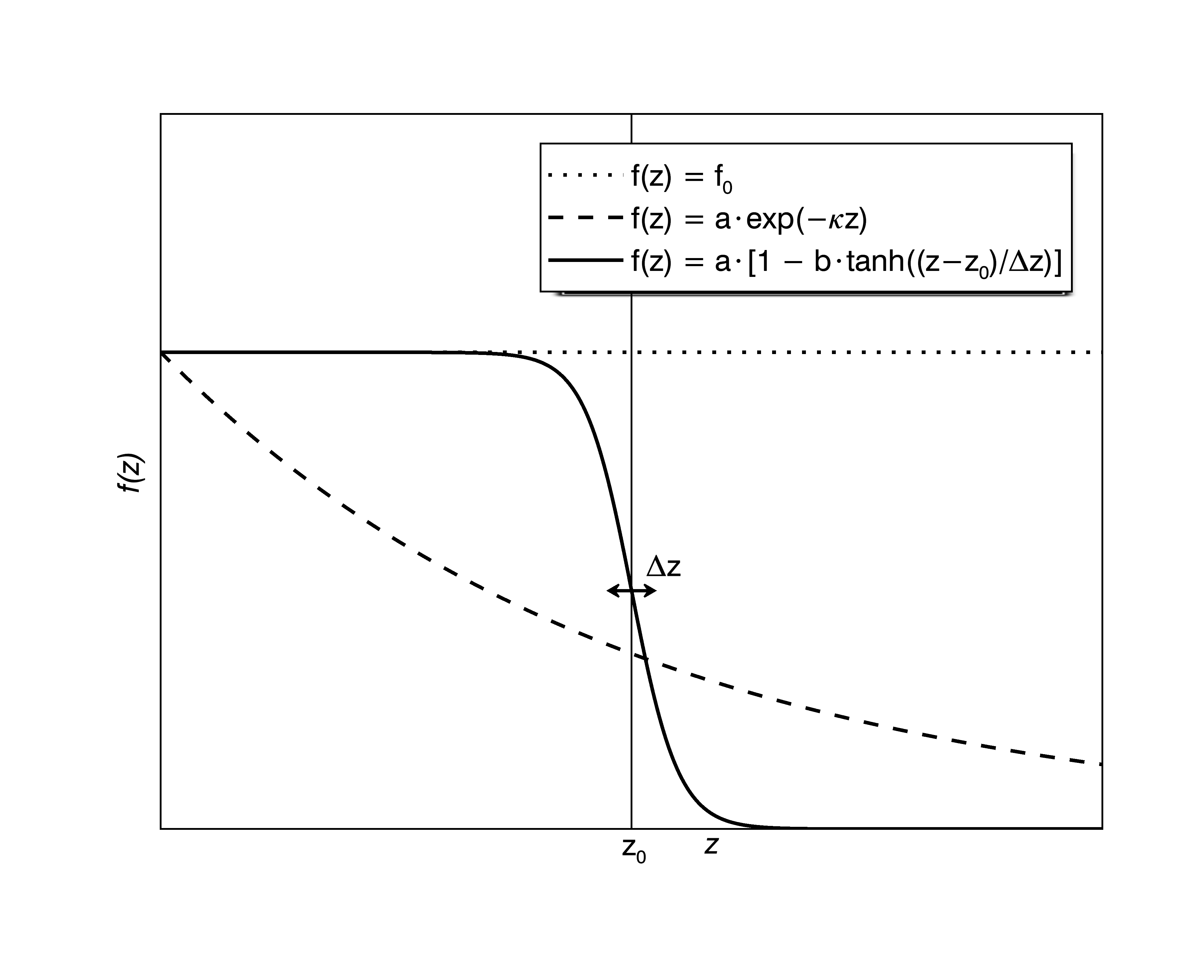
Figure 1.: The shape of $f(z)$ (solid line) defined in Equation eq:eckart-f-def. Also shown are the two limiting cases described in the main text.fig:fofz

We remark that the form of $f(z)$ in Equation eq:eckart-f-def includes the possibility of $f(z)=f_{0}=\mbox{constant}$, by choosing $b=0$. As discussed above, for this special case the $z$-dependence of the solutions is given by exponential functions (e.g. Neukirch, 1997a; Petrie, 2000; Petrie and Neukirch, 2000). In principle, Equation eq:eckart-f-def also includes the case of an exponentially decaying function of $z$ (e.g. Low, 1991) by choosing $b=1$ and letting

$$\lim\limits_{z_{0}\to-\infty}a\exp(2z_{0}/\Delta z)=\bar{a}>0.\ilabel{eq:exp-limit}$$ (21)

As stated above, in this case the $z$-dependence is given by Bessel functions with exponential arguments of the form $\exp(-\kappa z/2)$, with $\kappa/2=1/(\Delta z)$ in our limit (see e.g. Low, 1991). However, as one can see from the expression inside the limit, this case combines two of the parameters of $f$ into one parameter $\bar{a}$ and hence has less flexibility in applications. Although, as discussed before, the model with an exponential $f(z)$ also allows for a transition from non-force-free to force-free fields one can only control the length scale over which this happens, but one does not have an additional specific height at which this happens such as $z_{0}$ in the $f$ considered in this paper. We show example plots of the three different forms of $f(z)$ discussed above in Figure fig:fofz.

Substituting the function $f(z)$ given in Equation eq:eckart-f-def into Equation eq:Phibarequation we obtain:

$$\frac{{\mathrm{d}}^{2}\bar{\Phi}}{{\mathrm{d}}{z}^{2}}+\left[\alpha^{2}-k^{2}(1-a)-k^{2}ab\tanh\left(\frac{z-z_{0}}{\Delta z}\right)\right]\bar{\Phi}=0,\ilabel{eq:Phibar-eckart-equation}$$ (22)

Making use of the coordinate transformation

$$\eta=\frac{1}{2}\left[1-\tanh\left(\frac{z-z_{0}}{\Delta z}\right)\right]\ilabel{eq:eckart-transform}$$ (23)

with $0<\eta<1$, we can transform Equation eq:Phibar-eckart-equation into the differential equation

$$\frac{{\mathrm{d}}^{2}\bar{\Phi}}{{\mathrm{d}}{\eta}^{2}}+\left(\frac{1}{\eta}-\frac{1}{1-\eta}\right)\frac{{\mathrm{d}}\bar{\Phi}}{{\mathrm{d}}\eta}+\left(\frac{C_{1}}{\eta}-\frac{C_{2}}{1-\eta}\right)\frac{\bar{\Phi}}{\eta(1-\eta)}=0,\ilabel{eq:Phibar-hypergeometric-equation}$$ (24)

where

$$C_{1} = \frac{1}{4}\left[{\bar{k}}^{2}(1-a+ab)-{\bar{\alpha}}^{2}\right],$$ (25)

$$C_{2} = \frac{1}{4}\left[{\bar{k}}^{2}(1-a-ab)-{\bar{\alpha}}^{2}\right],$$ (26)

with $\bar{k}=k\Delta z$ and $\bar{\alpha}=\alpha\Delta z$. Equation eq:Phibar-hypergeometric-equation can be solved using the hypergeometric function ${~{}}_{2}{\mathrm{F}}_{1}(a,b,c;z)$ (see e.g. Abramowitz and Stegun, 1965; Olver et al., 2010) in the form

$$\bar{\Phi}= \mbox{}A\eta^{\delta}(1-\eta)^{\gamma}{~{}}_{2}{\mathrm{F}}_{1}(\gamma+\delta+1,\gamma+\delta,2\delta+1;\eta)+$$ (27)

$$\mbox{}B\eta^{-\delta}(1-\eta)^{\gamma}{~{}}_{2}{\mathrm{F}}_{1}(\gamma-\delta+1,\gamma-\delta,1-2\delta;\eta),$$

with $\gamma=\sqrt{C_{2}}$, $\delta=\sqrt{C_{1}}$, and $A$, $B$ constants to be determined by boundary conditions at $z=z_{\mathrm{min}}$ (here we take $z_{\mathrm{min}}=0$) and $z=z_{\mathrm{max}}$. For example, if we want the solution to tend to zero as $z\to\infty$ ($\eta\to 0$), we have to choose $B=0$. The other coefficient $A$ will be determined by the boundary condition at $z=z_{\mathrm{min}}=0$ in the same way as in the potential or linear force-free magnetic field case. The only difference is the functional dependence of the individual modes on $z$.

We notice that for given values of $a$, $b$ and $\bar{\alpha}$ the parameters $C_{1}$ and $C_{2}$ become negative for small $k$ (in particular $C_{1}<0$ if $\bar{k}^{2}<\bar{\alpha}^{2}/[1-a(1-b)]$ and $C_{2}<0$ when $\bar{k}^{2}<\bar{\alpha}^{2}/[1-a(1+b)]$). This implies that $\gamma$, $\delta$ or both become imaginary. The change in nature of the solution is similar to the change from exponential to trigonometric in the linear force-free case and while this can in principle be incorporated into a Green’s function approach (for a discussion see e.g. Chiu and Hilton, 1977; Wheatland, 1999; Petrie and Lothian, 2003; Priest, 2014) one usually has to impose restrictions on the values of $a$, $b$ and $\bar{\alpha}$ in the case with periodic boundary conditions and discrete Fourier modes. As in the linear force-free case the specific bounds are determined by the smallest value of the wave vector $k^{2}$. We will discuss an example in section sec:examples.

4 Illustrative Examples

sec:examples

Instead of using an arbitrary magnetogram we investigate the effects of the solution parameters on the structure of the magnetic field and the plasma pressure, density and temperature, by using a relatively simple, doubly periodic example which allows us to control the shape of the bottom boundary conditions and hence enables us to undertake a study of the solutions that highlights the features of the solutions more clearly.

To achieve this we will use the following boundary condition for $B_{z}$ at $z=0$:

$$B_{z}(x,y,0) = B_{0}\left\{\frac{\exp\left[\tilde{\kappa}_{x1}\cos\left(\tilde{x}-\tilde{\mu}_{x1}\right)\right]}{2\pi\mbox{I}_{0}(\tilde{\kappa}_{x1})}\frac{\exp\left[\tilde{\kappa}_{y1}\cos\left(\tilde{y}-\tilde{\mu}_{y1}\right)\right]}{2\pi\mbox{I}_{0}(\tilde{\kappa}_{y1})}\right.$$ (28)

$$\mbox{\hskip 14.22636pt}\left.-\frac{\exp\left[\tilde{\kappa}_{x2}\cos\left(\tilde{x}-\tilde{\mu}_{x2}\right)\right]}{2\pi\mbox{I}_{0}(\tilde{\kappa}_{x2})}\frac{\exp\left[\tilde{\kappa}_{y2}\cos\left(\tilde{y}-\tilde{\mu}_{y2}\right)\right]}{2\pi\mbox{I}_{0}(\tilde{\kappa}_{y2})}\right\}.$$

This choice is based on a special case of the bivariate von Mises distribution which is used, for example, in directional statistics (see e.g. Mardia and Jupp, 1999) and we combine two of these functions, one with a positive sign and one with a negative sign, to balance the magnetic flux through the lower boundary. Here $\tilde{x}=\pi x/L$ and $\tilde{y}=\pi y/L$, with the domain size in the $x$- and $y$-directions given by $-1\leq\tilde{x},\,\tilde{y}\leq 1$. All other quantities with a tilde that are directly related to length scales are also normalised by $L$. Furthermore, $B_{0}$ is a reference magnetic field value, the $\tilde{\kappa}_{ij}\,\,(>0)$ values determine the width of the flux distribution, with larger $\tilde{\kappa}_{ij}$ values making the width to smaller, the $\tilde{\mu}_{ij}$ values specify the positions of the maximum or minimum of the magnetic flux distribution. The function $\mbox{I}_{0}(x)$ is a modified Bessel function of the first kind (see e.g. Abramowitz and Stegun, 1965; Olver et al., 2010). The denominator is included to normalise the integral of the bivariate von Mises distribution over the $x$-$y$ box to unity, so that the positive and the negative magnetic flux through the bottom boundary cancel exactly and the total magnetic flux through the bottom boundary vanishes, independently of the values chosen for $\tilde{\kappa}_{ij}$ and $\tilde{\mu}_{ij}$. The remaining boundary condition imposed is $B_{z}\to 0$ as $z\to\infty$.

  

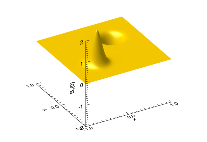
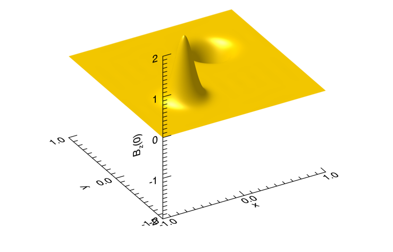
(a)                                      (b)

Figure 2.: Surface plot of the $B_{z}$-component of the magnetic field at $z=0$ used for the examples in this paper. Panel (a) shows a plot of the exact expression eq:magnetogram and panel (b) an approximation based on a Fourier expansion using ten Fourier modes. The parameter values used in this plot are $\tilde{\mu}_{x1}=\tilde{\mu}_{y1}=-\tilde{\mu}_{x2}=-\tilde{\mu}_{y2}=1.2/\pi\approx 0.382$ and $\kappa_{x1}=\kappa_{x2}=\kappa_{y1}=\kappa_{y2}=10$. The maximum value of $|B_{z}|/B_{0}$ in this plot is $\approx\exp(2\tilde{\mu}_{x1})/[2\pi\mbox{I}_{0}(\tilde{\kappa}_{x1})]^{2}=1.55$. The difference between the exact plot and the ten-mode approximation is of the order of $10^{-5}$.fig:magnetogram

The function eq:magnetogram is periodic in the $x$- and the $y$-direction and can easily be expanded into a Fourier series, which allows us to find the general solution for these boundary conditions without problems (for mathematical details see Appendix app:fourier). We show surface plots of the exact expression eq:magnetogram and an expansion based on the first ten Fourier modes in both $x$ and $y$ in Figure fig:magnetogram. The parameter values used in this plot are $\tilde{\mu}_{x1}=\tilde{\mu}_{y1}=-\tilde{\mu}_{x2}=-\tilde{\mu}_{y2}=1.2/\pi\approx 0.382$ and $\kappa_{x1}=\kappa_{x2}=\kappa_{y1}=\kappa_{y2}=10$. The maximum difference between the exact plot and the ten-mode approximation is of the order of $10^{-5}$ and hence the ten-mode approximation is considered to be sufficiently accurate for this choice of parameter values.

For the MHS examples we will be showing we have used the values $z_{0}=0.2L$, $\Delta z=0.1z_{0}$ and $b=1.0$, which means that for $z\gg z_{0}$ the magnetic field tends towards a potential state (in the case $\alpha=0$) or a linear force-free state (if $\alpha\neq 0$). By choosing $b<1.0$ one could retain a controlled level of MHS behaviour of the magnetic field above $z_{0}$.

We will present solutions for different values of the parameter $a$ below the maximum value for $a$, which is given by

$$a_{\mathrm{max}}=\frac{\bar{k}^{2}_{\mathrm{min}}-\bar{\alpha}^{2}}{\bar{k}^{2}_{\mathrm{min}}(1+b)}.\ilabel{eq:amax}$$ (29)

As discussed in Section sec:solutions the condition eq:amax follows directly from the definition of $\gamma$ and for given $b$, $\alpha$ and minimum value of $k^{2}$ corresponds to the value of $a$ at which $\gamma$ becomes imaginary. One can also see from Equation eq:amax that to have $a_{\mathrm{max}}>0$ one has to have $k^{2}_{\mathrm{min}}>\alpha^{2}$ which is the condition for linear force-free field modes to drop off exponentially with height.

  

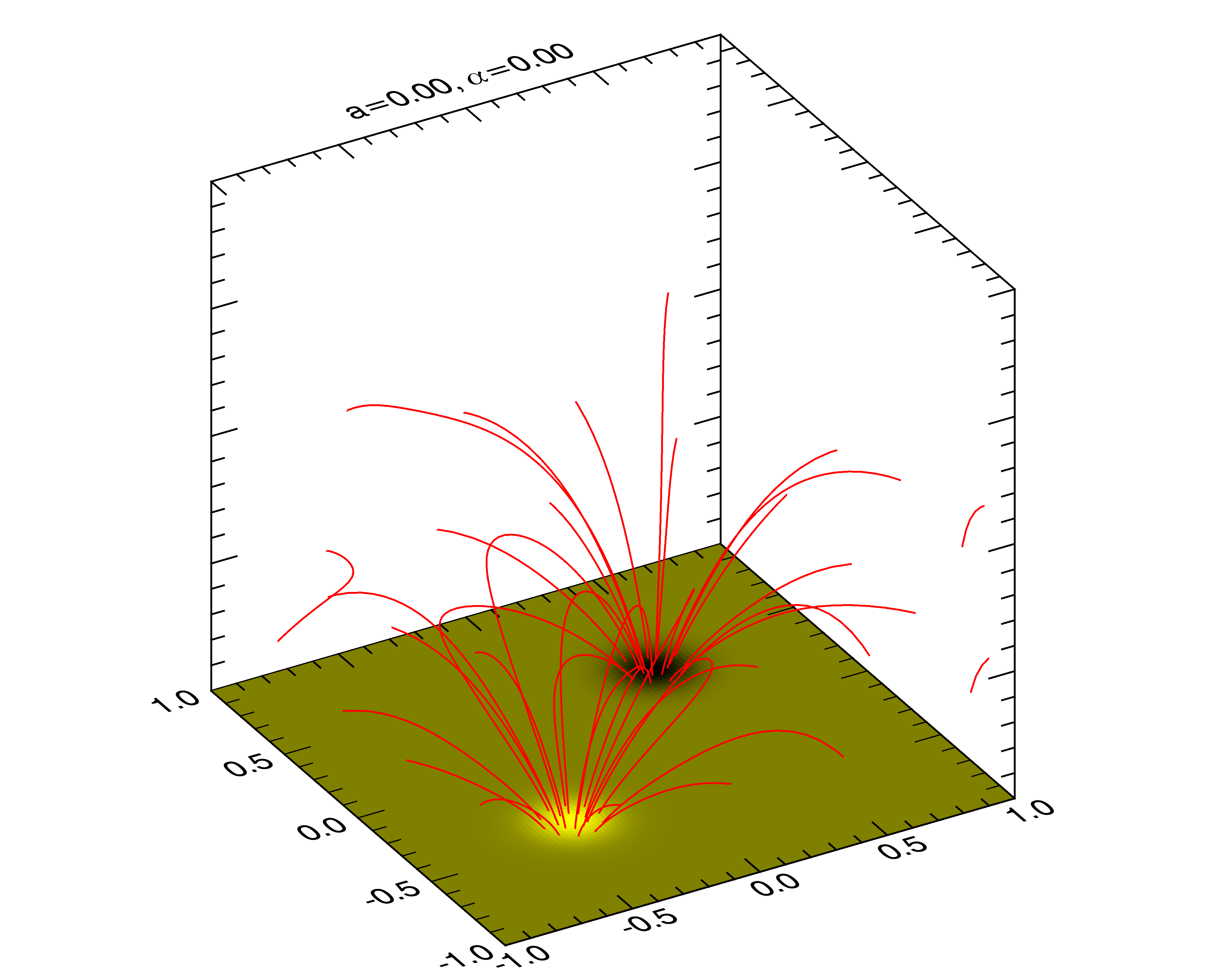
(a)                                      (b)

  

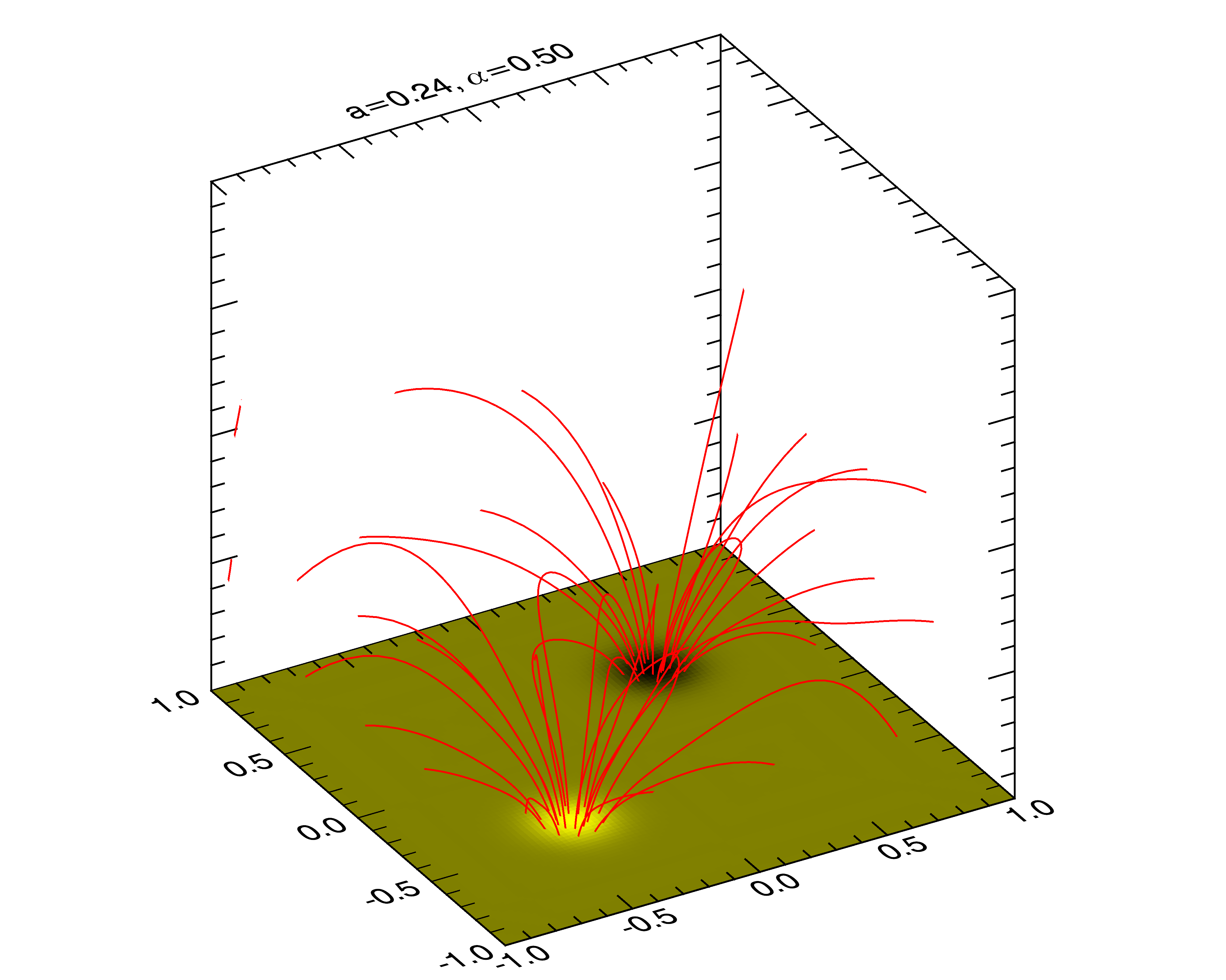
(c)                                      (d)

Figure 3.: Field line plots for the boundary conditions shown in Figure fig:magnetogram. The box is a cube with size is $-1\leq x/L,\,y/L\leq 1$, $0\leq z/L\leq 2$. Panel (a) shows the potential magnetic field ($a=0$, $\tilde{\alpha}=0$), panel (b) a linear force-free magnetic field ($a=0$, $\tilde{\alpha}=0.5$) and panels (c) and (d) two MHS solutions with $a=0.24$, $\tilde{\alpha}=0.5$, in panel (c) and $a=0.48$, $\tilde{\alpha}=0.5$, in panel (d). In each panel we show field lines traced from the same foot points located on two concentric circles around the position of the positive polarity maximum. The field lines are traced until the encounter the lower boundary, with the periodic boundary conditions are taken into account.fig:B-perspective

    

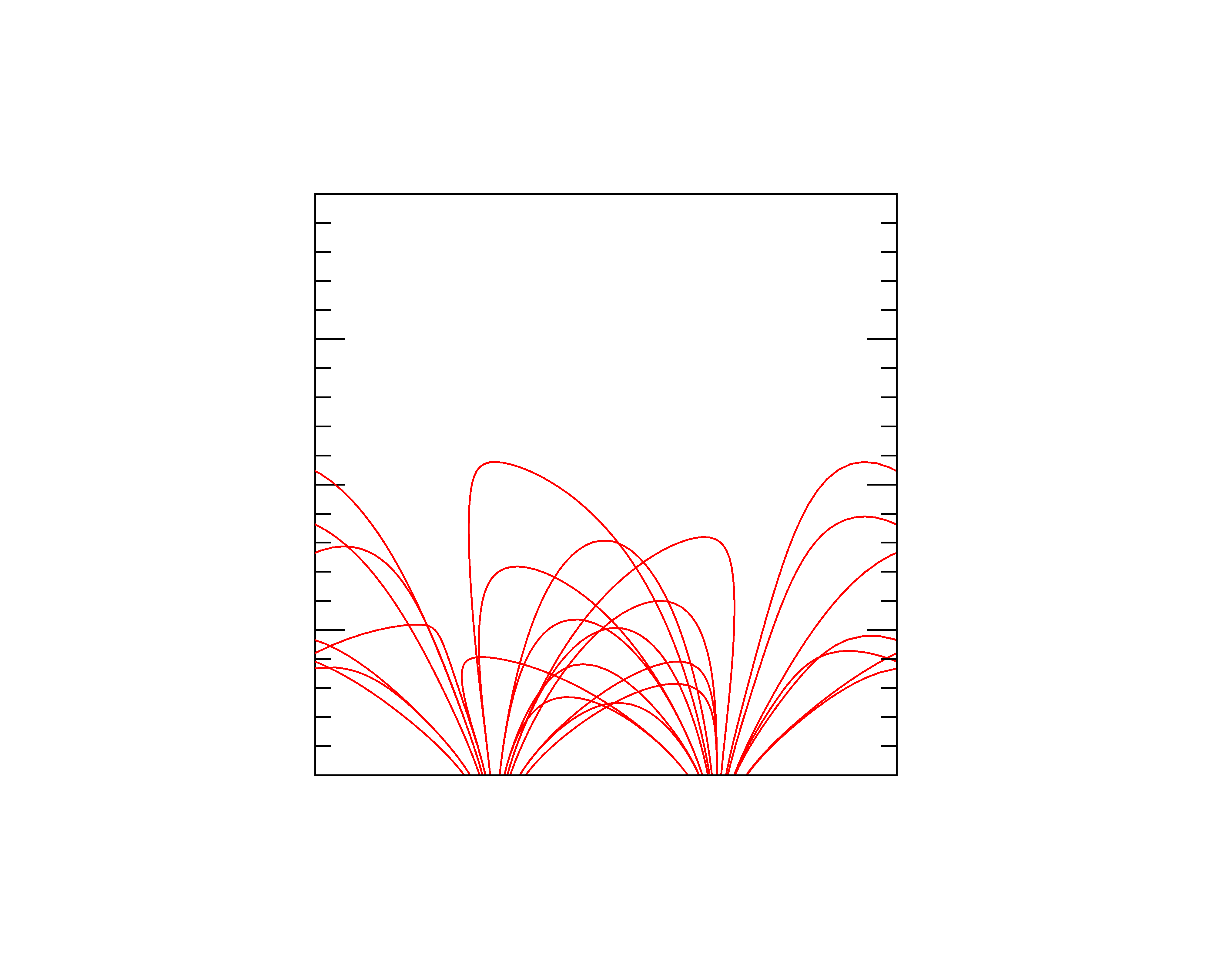
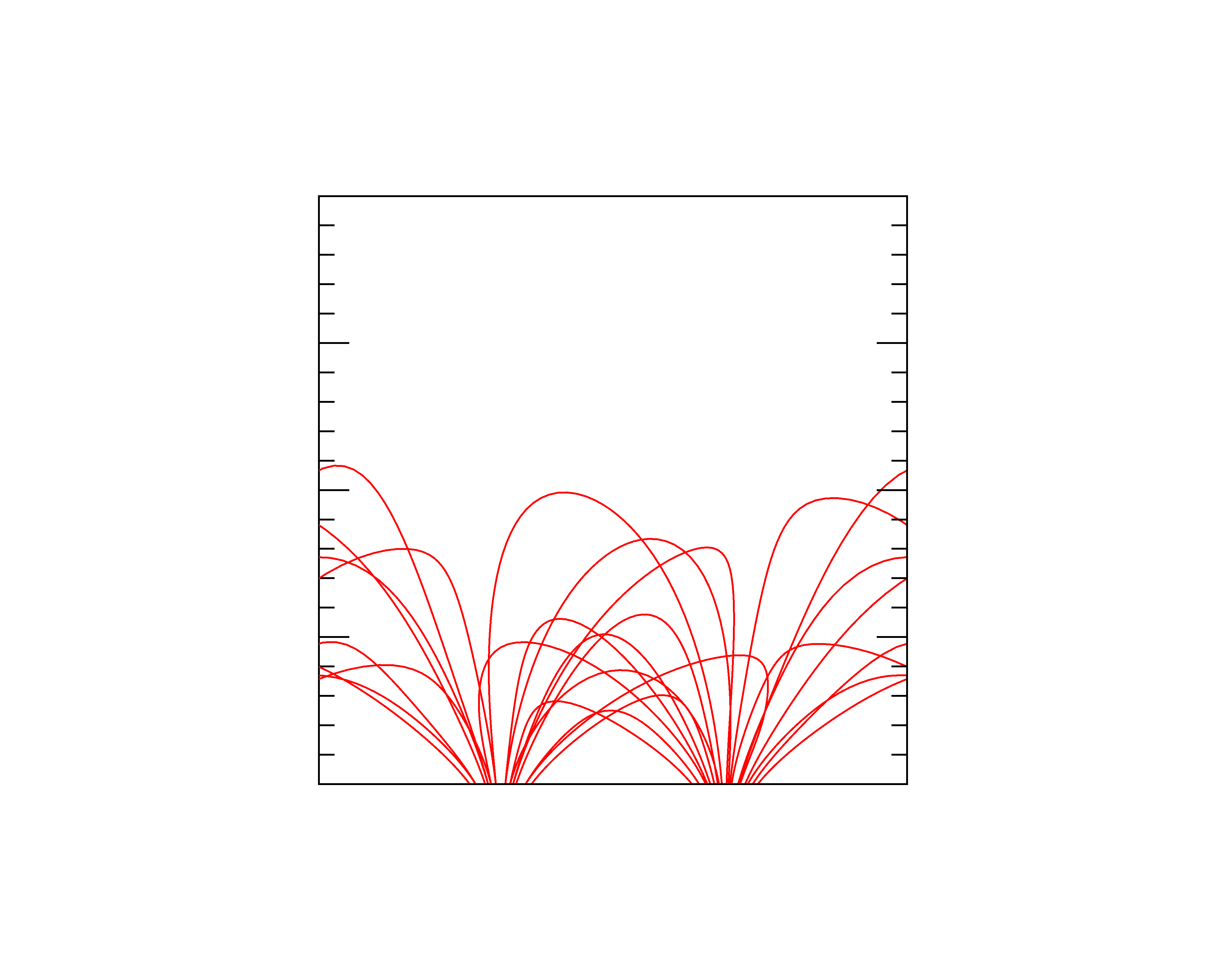
        (a)                                      (b)

    

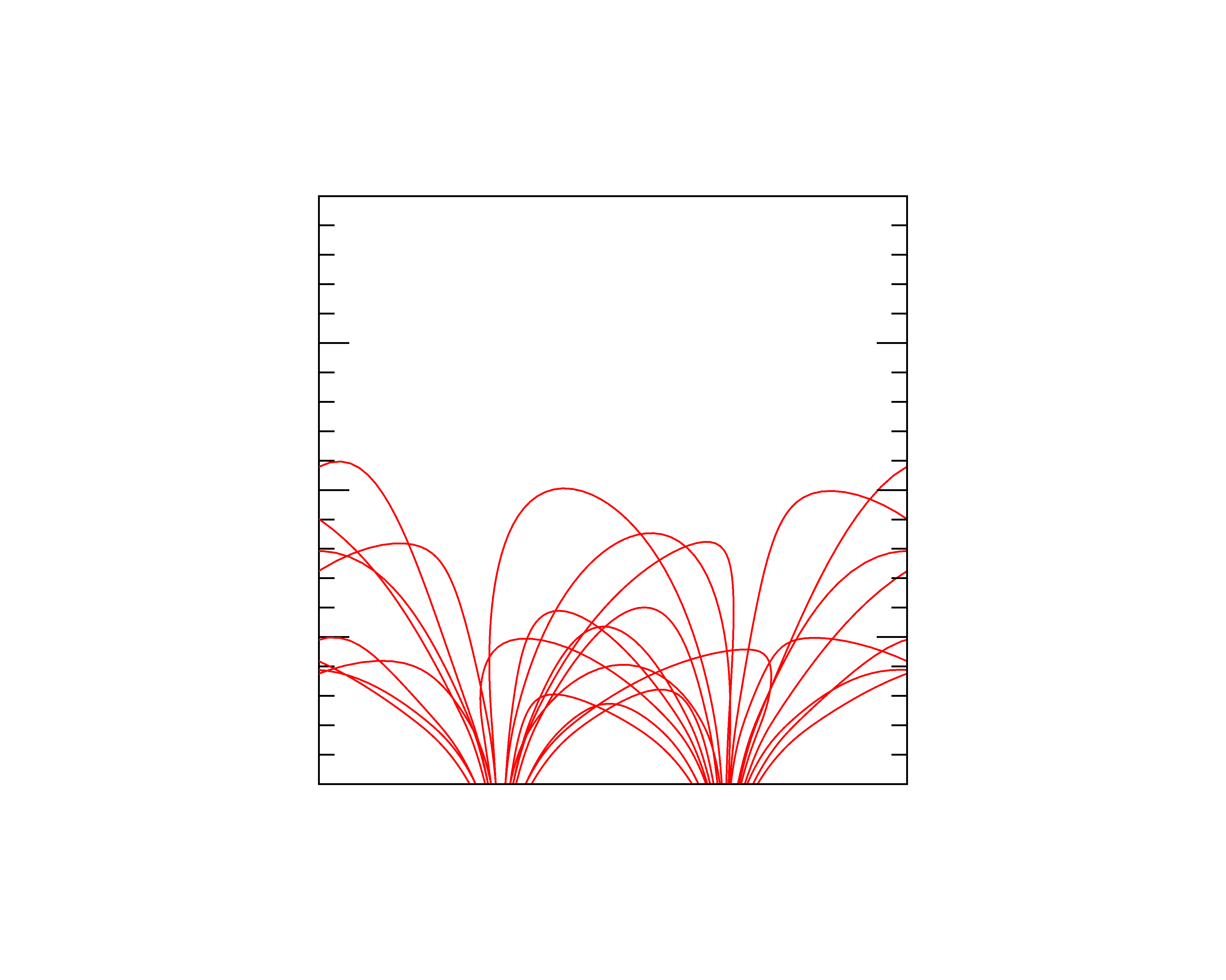
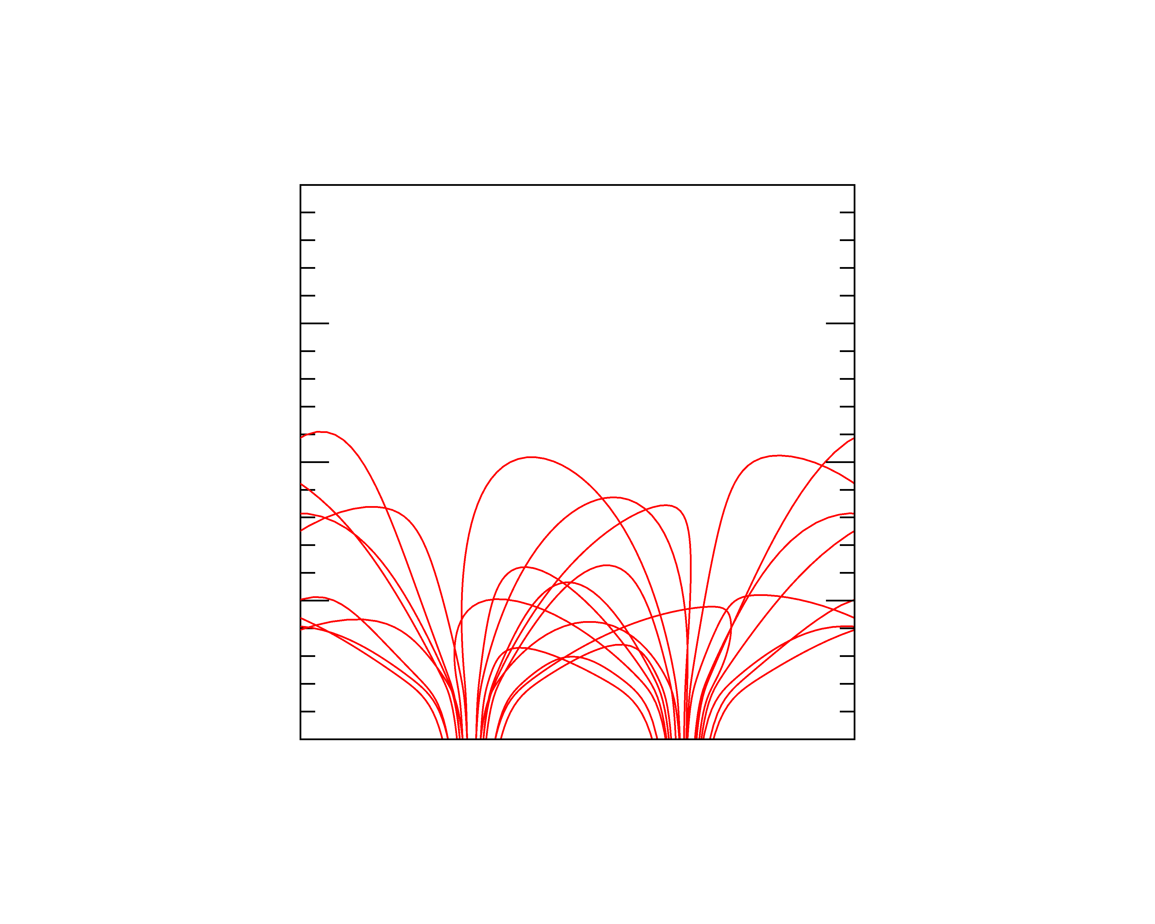
        (c)                                      (d)

Figure 4.: The same field line plots as in Figure fig:B-perspective, but viewed along the $y$-direction (i.e. projected onto the $x$-$z$-plane). As in Figure fig:B-perspective we have $-1\leq x/L\leq 1$ (horizontal direction) and $0\leq z/L\leq 2$ (vertical direction). The field lines in the MHS cases (panels (c) and (d)) show clear signs of steepening below $z/L=z_{0}/L=0.2$ (second tickmark on the vertical $z$-axis), as expected.fig:B-sideview

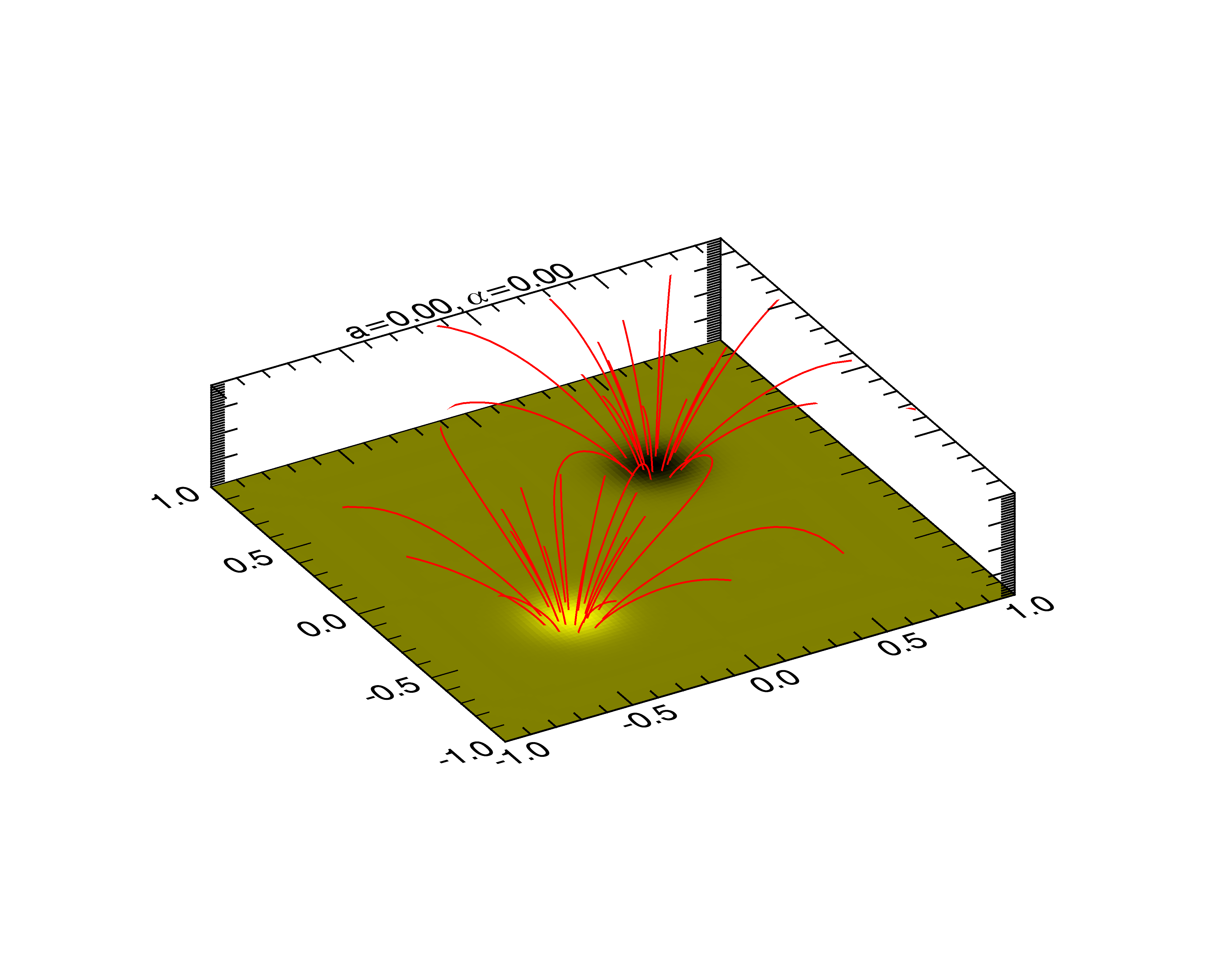
(a)                                              (b)

      

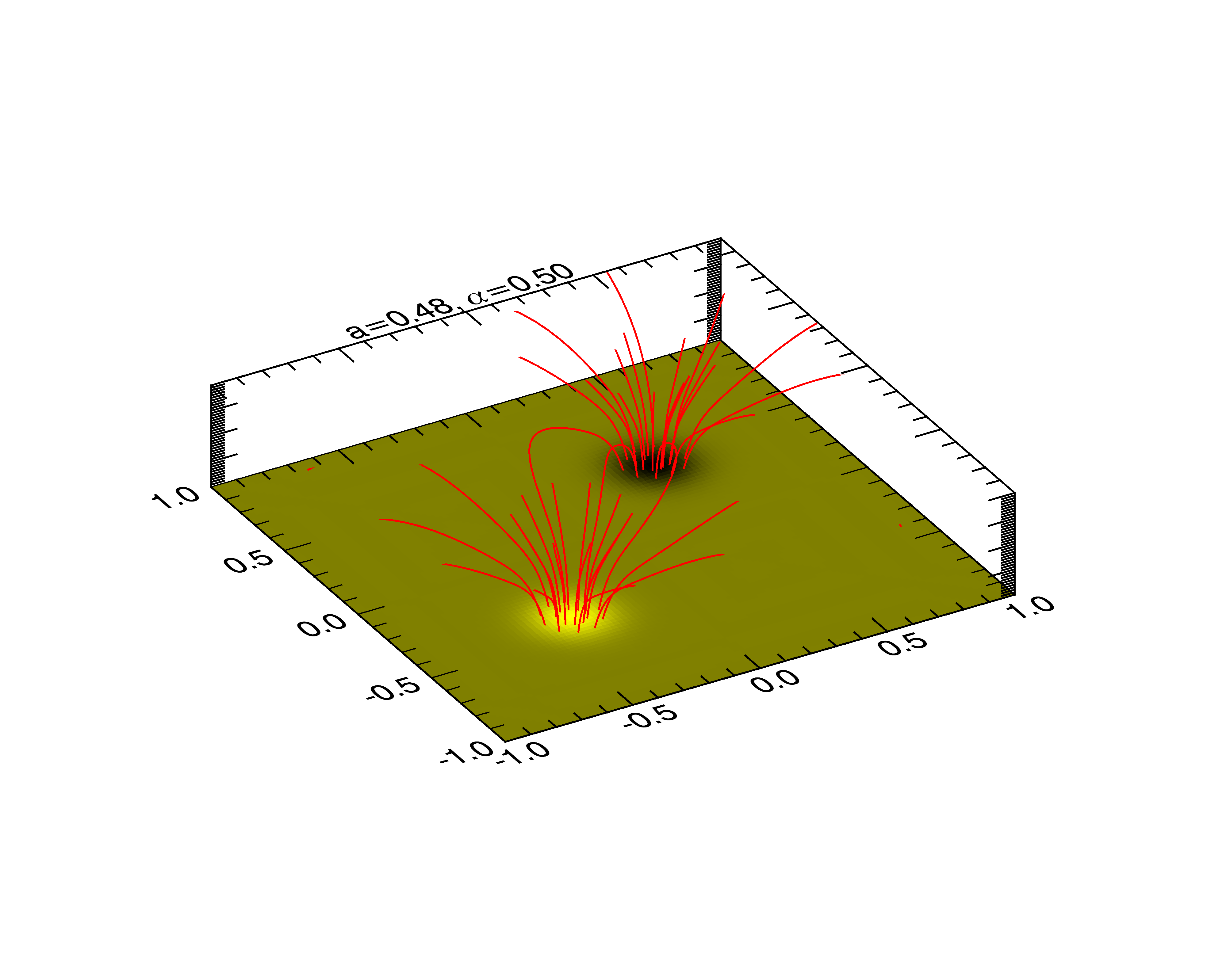
(c)                                              (d)

Figure 5.: The same field line plots as in Figure fig:B-perspective, but with $0\leq z\leq 2z_{0}$ to make the difference between the various cases more obvious.fig:B-perspective-lowb

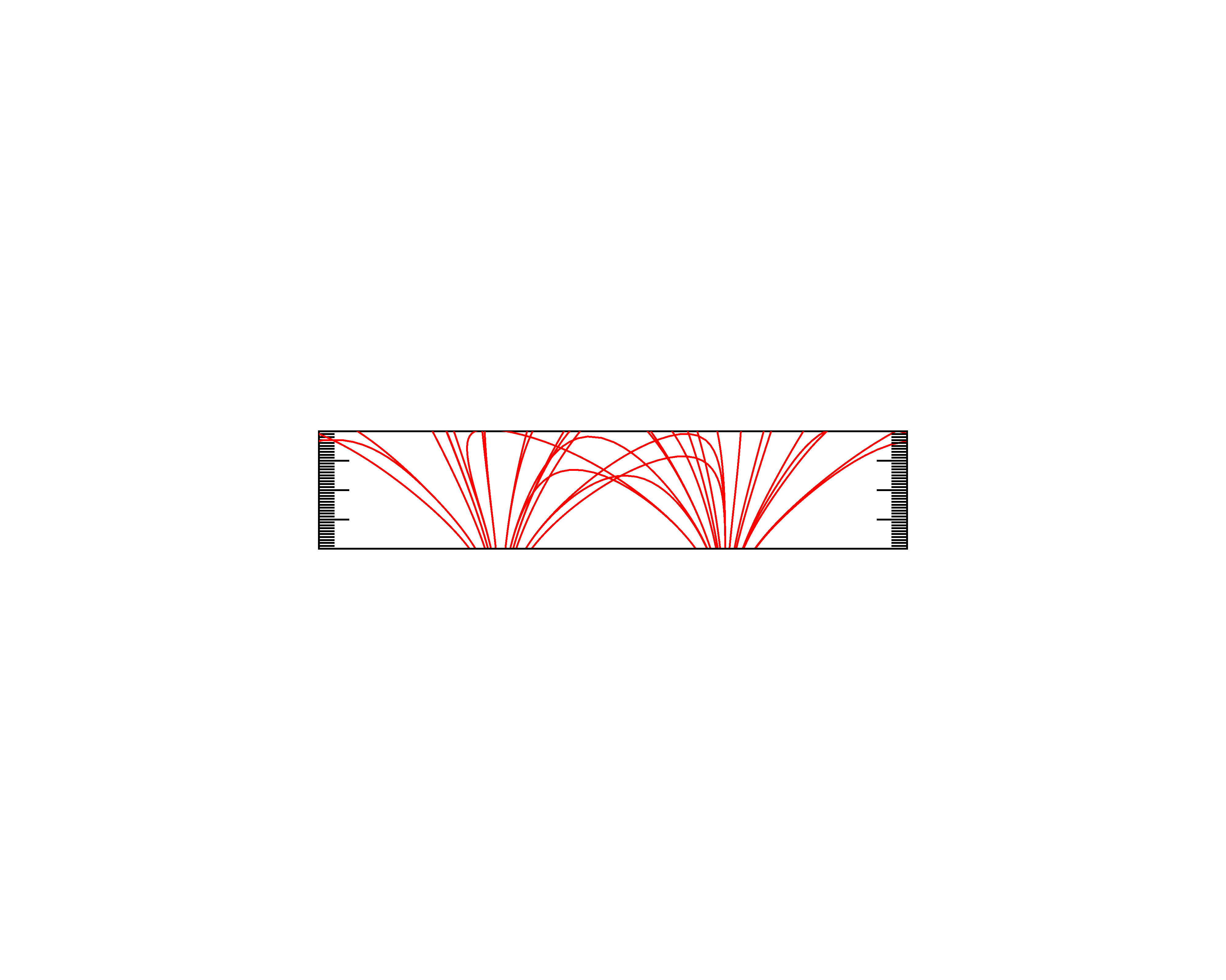
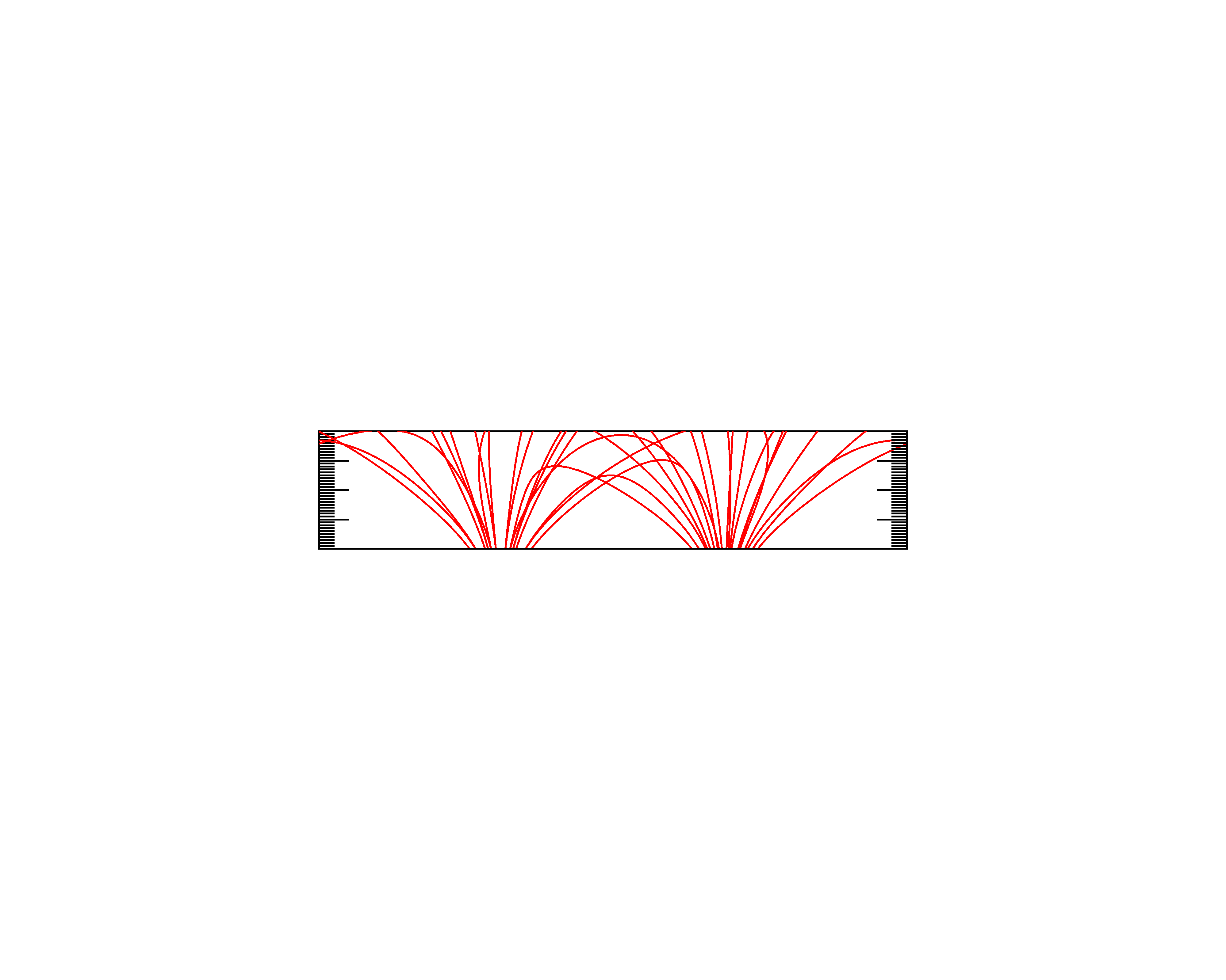
      (a)                                     (b)

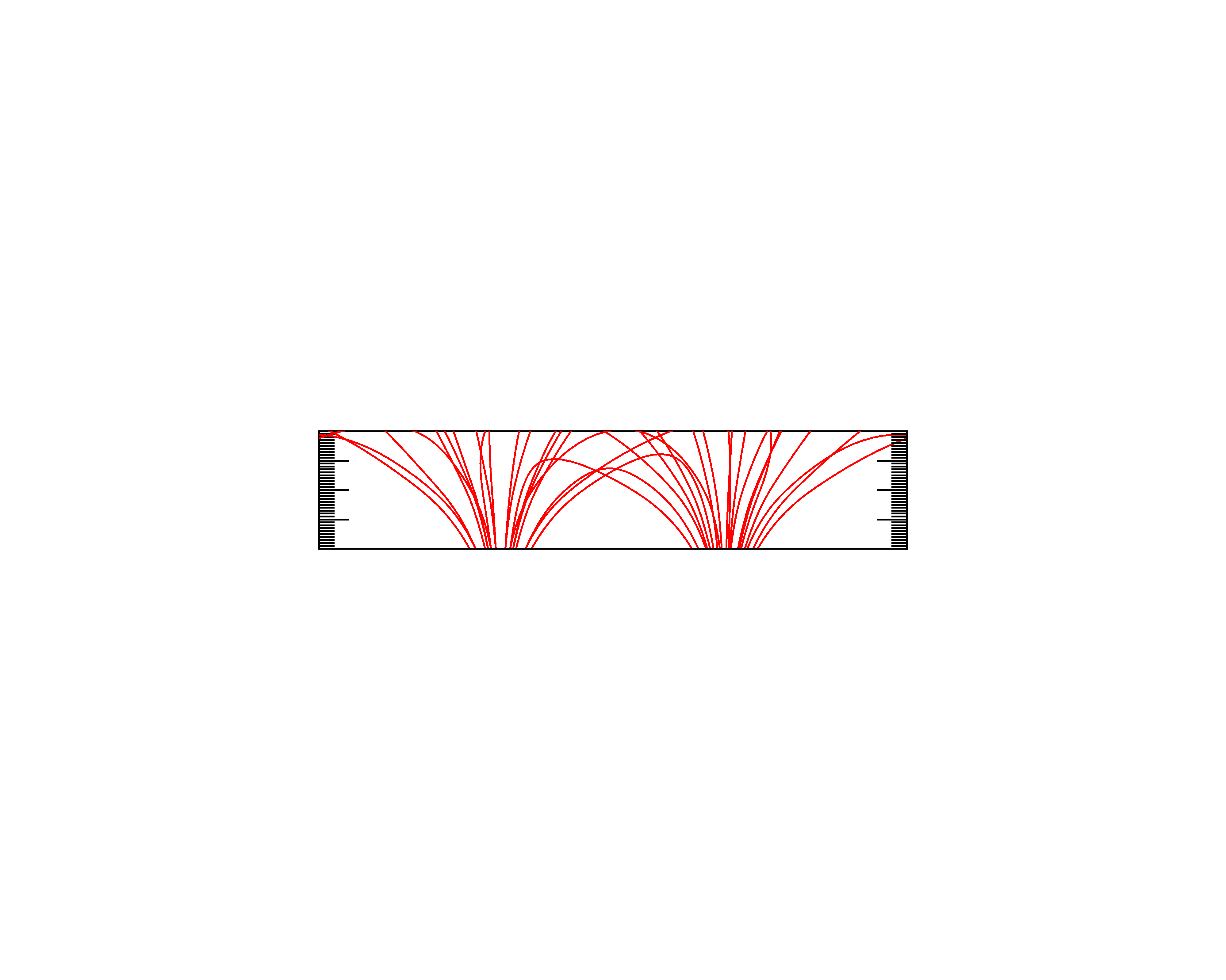
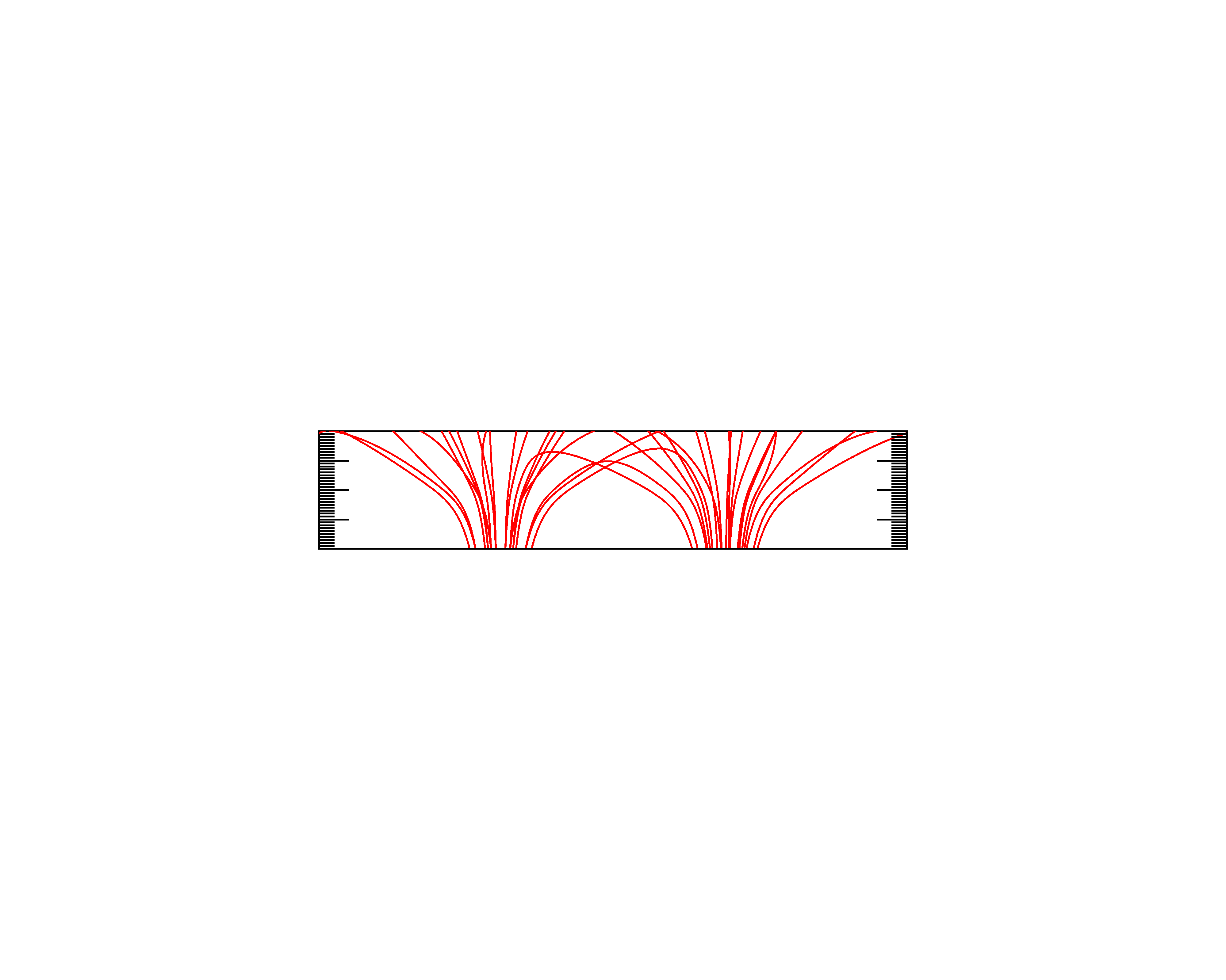
      (c)                                     (d)

Figure 6.: The same field line plots as in Figure fig:B-perspective-lowb, but viewed along the $y$-direction (i.e. projected onto the $x$-$z$-plane).fig:B-sideview-lowb

We present magnetic field line plots for four different parameter combinations in Figures fig:B-perspective and fig:B-sideview. For reference we present the potential magnetic field for the given boundary conditions ($a=0.0$, $\alpha=0.0$) in panel (a) and the linear force-free magnetic field with $\alpha=0.5$ ($a=0$) in panel (b) of Figures fig:B-perspective and fig:B-sideview. We compare these two cases with two field line plots for non-zero values of $a$, one roughly half of $a_{\mathrm{max}}$ and the other $0.99\,a_{\mathrm{max}}$. To highlight the region where the field lines change the most between the different cases, we also present the same field line plots on a domain with $z\leq 2z_{0}$ in Figures fig:B-perspective-lowb and fig:B-sideview-lowb.

As expected, the main difference between the linear force-free case and the two MHS cases can be seen for $z\leq z_{0}$. This is particularly obvious in Figure fig:B-sideview, in which a considerable steepening of the field lines is noticeable in the region below $z_{0}=0.2$. This change in the field line behaviour can be attributed to the value of the smallest $\gamma$ in the series expansion approaching zero which leads to a less rapid decrease of the lowest order mode with height for $z\leq z_{0}$. Due to our choice of a relatively small value for $\Delta z$ this behaviour changes relatively sharply around $z\approx z_{0}$ and hence no major changes in the magnetic field can be seen at heights above $z_{0}$. The magnetic field above $z_{0}$ is therefore basically identical to a linear force-free field.

   

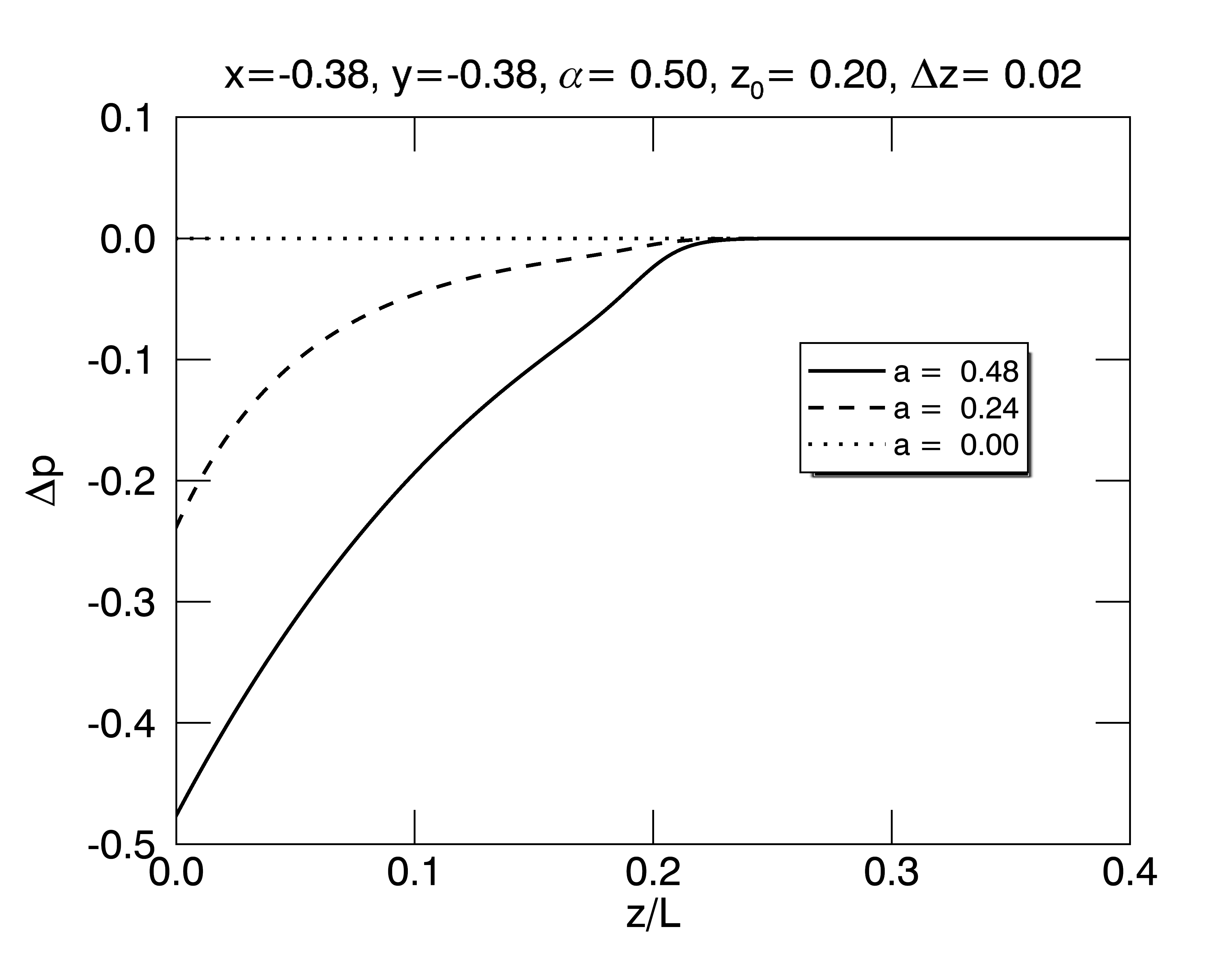
          (a)

   

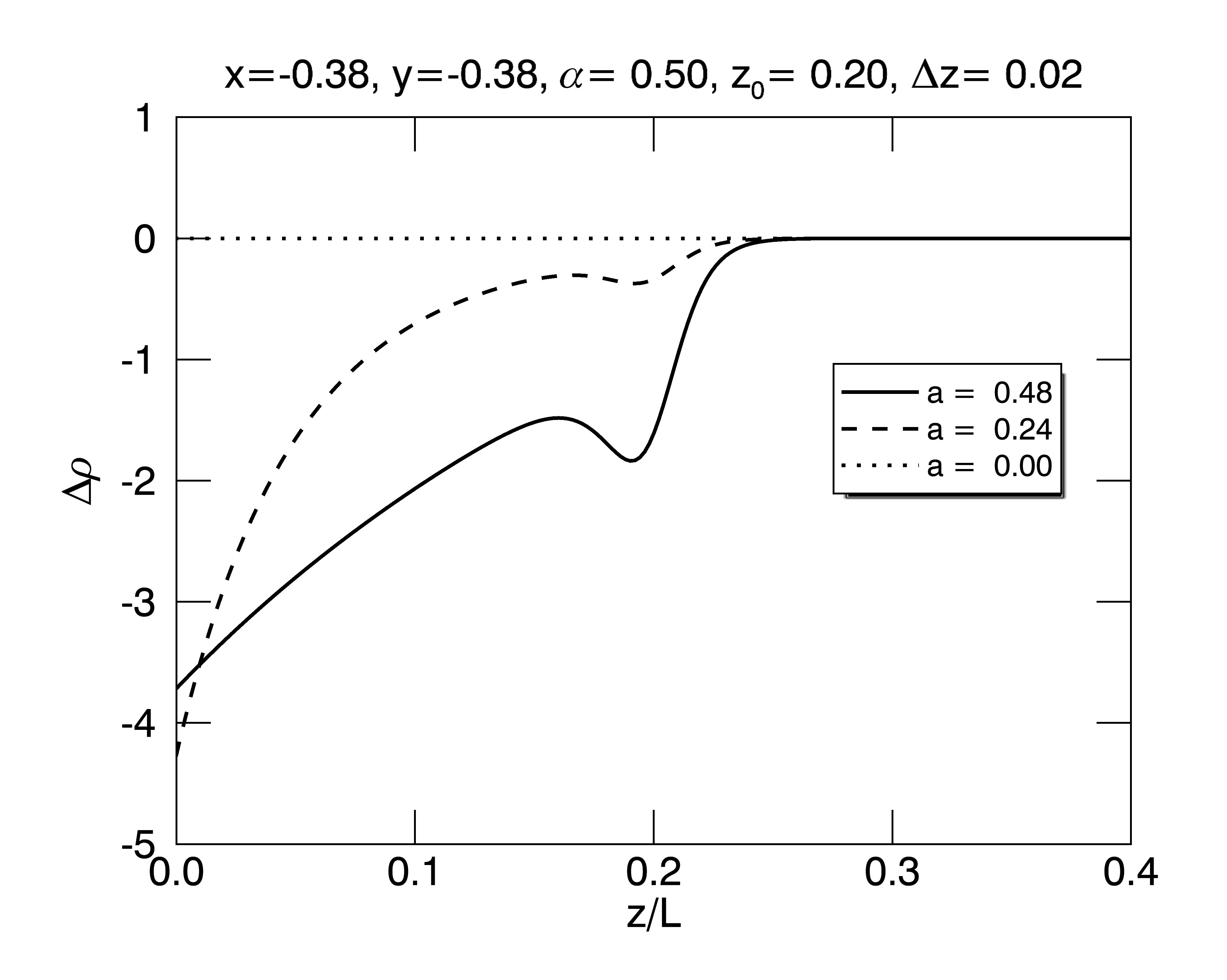
          (b)

Figure 7.: Plots of the variation with height $z$ of the pressure (panel (a)) and density (panel(b)) deviation from a stratified background atmosphere for $\alpha=0.5$, $z_{0}/L=0.2$ and $\Delta z=0.1z_{0}$, and three different values of $a$ ($a=0.0$, $0.24$ and $0.48$). The $x$- and $y$-coordinates of these plots are the position of the maximum value of $|B_{z}|$ on the lower boundary, $x/L=\mu_{x}/\pi\approx-0.38$, $y/L=\mu_{y}/\pi\approx-0.38$.fig:pandrho-lineplots

  

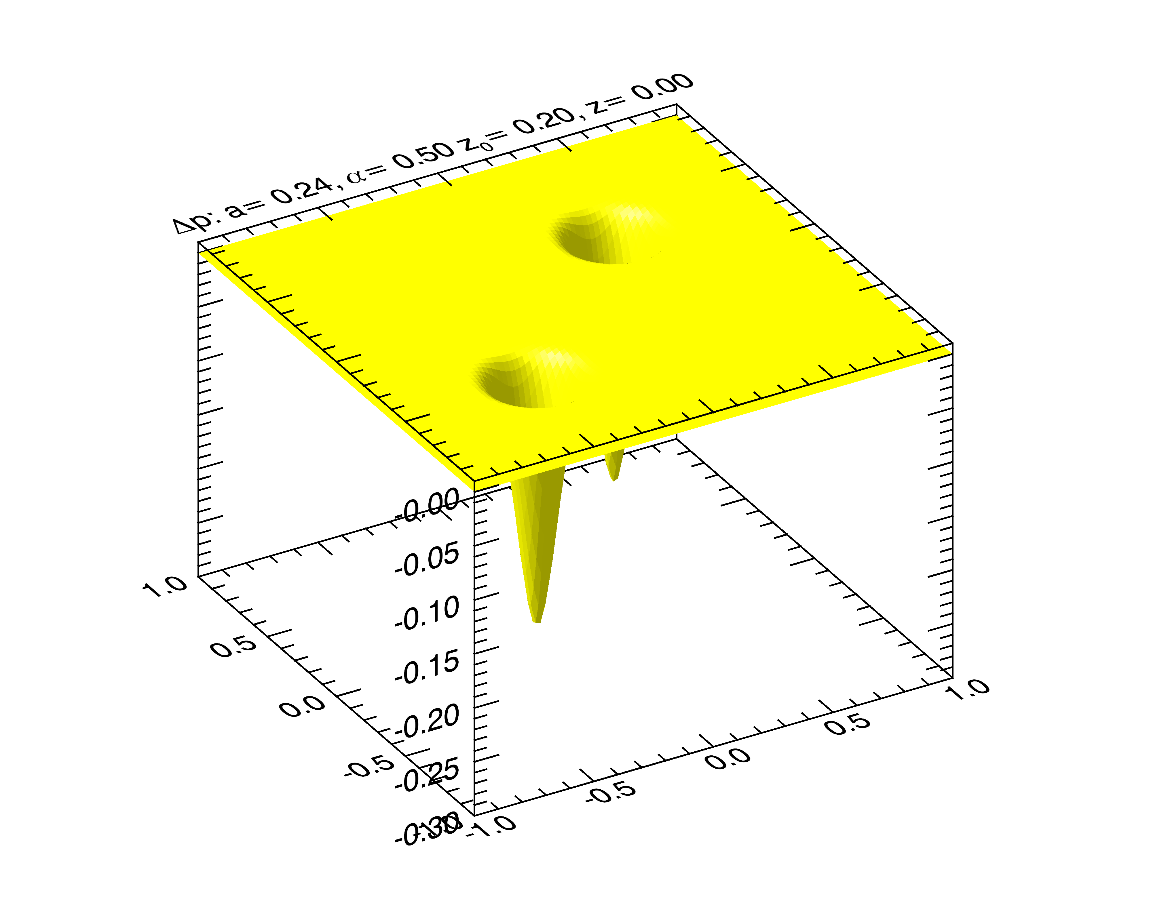
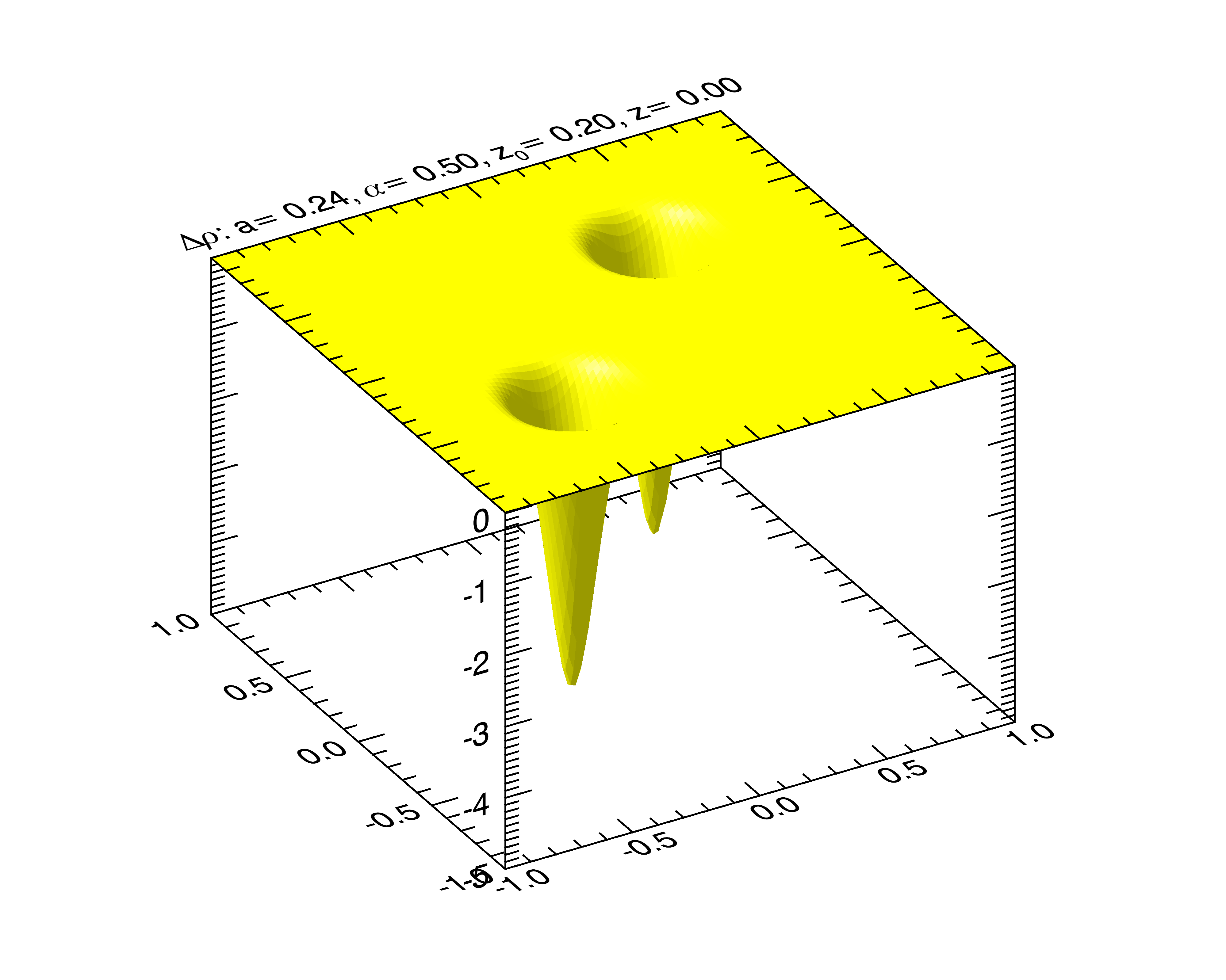
(a)                                      (b)

  

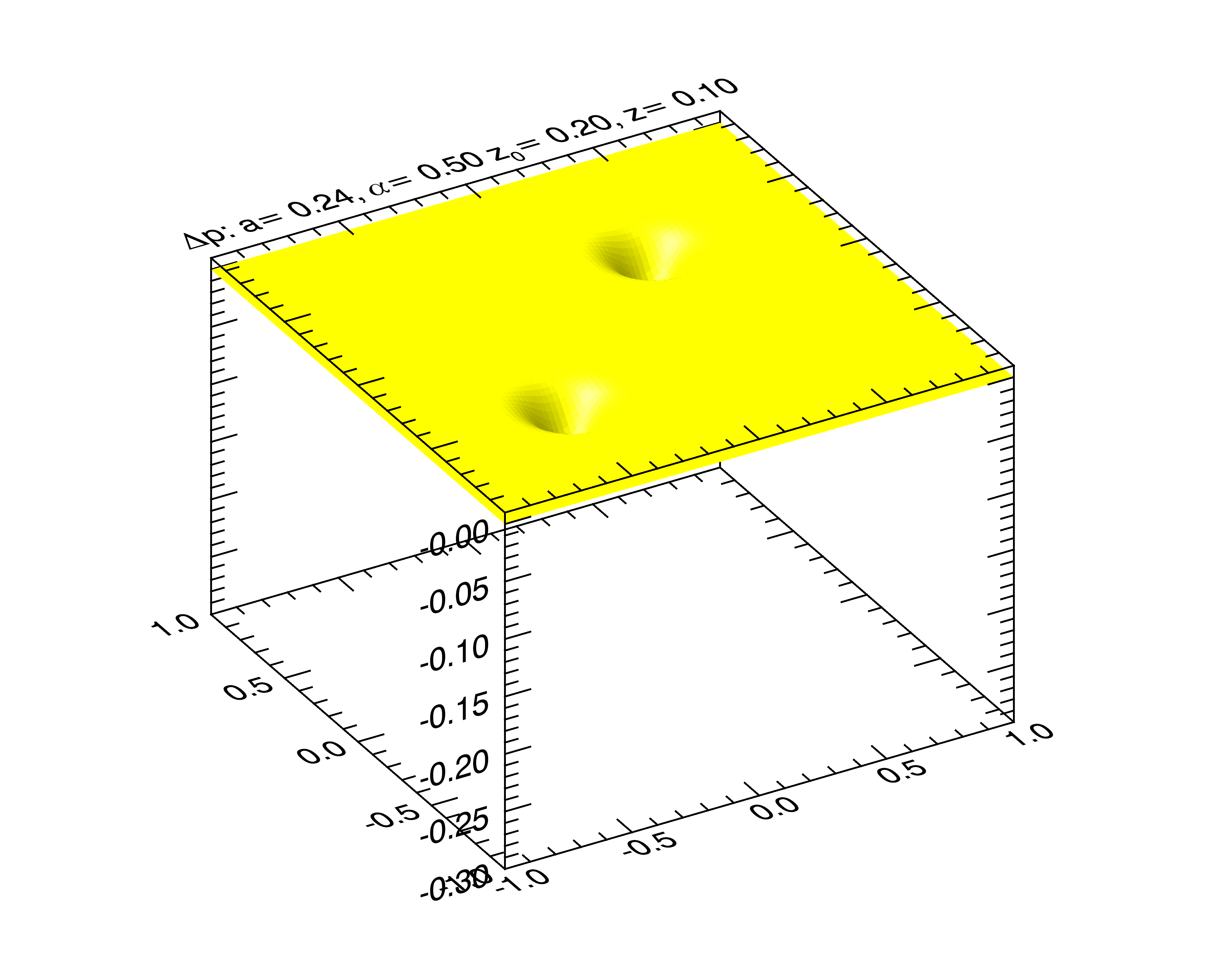
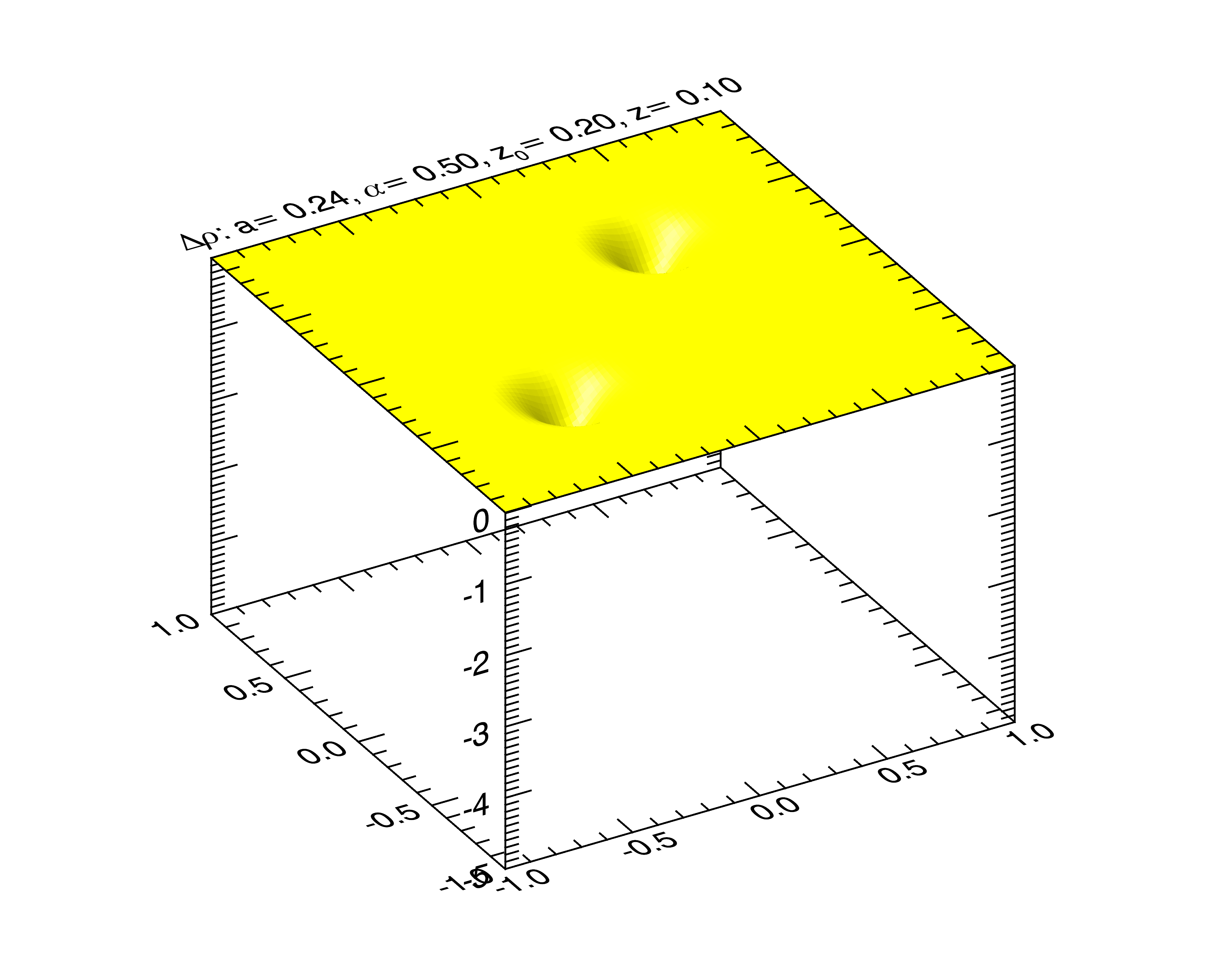
(c)                                      (d)

  

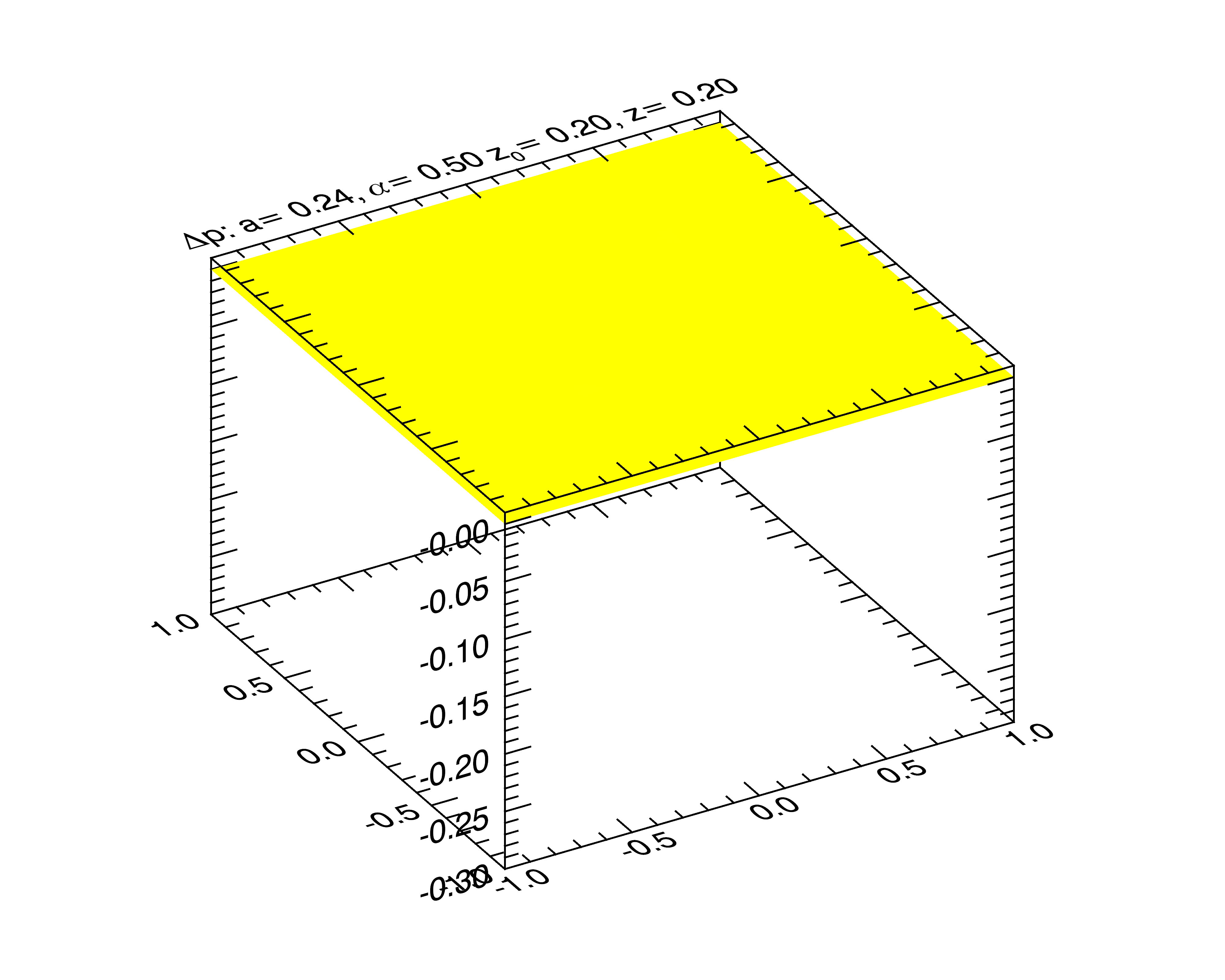
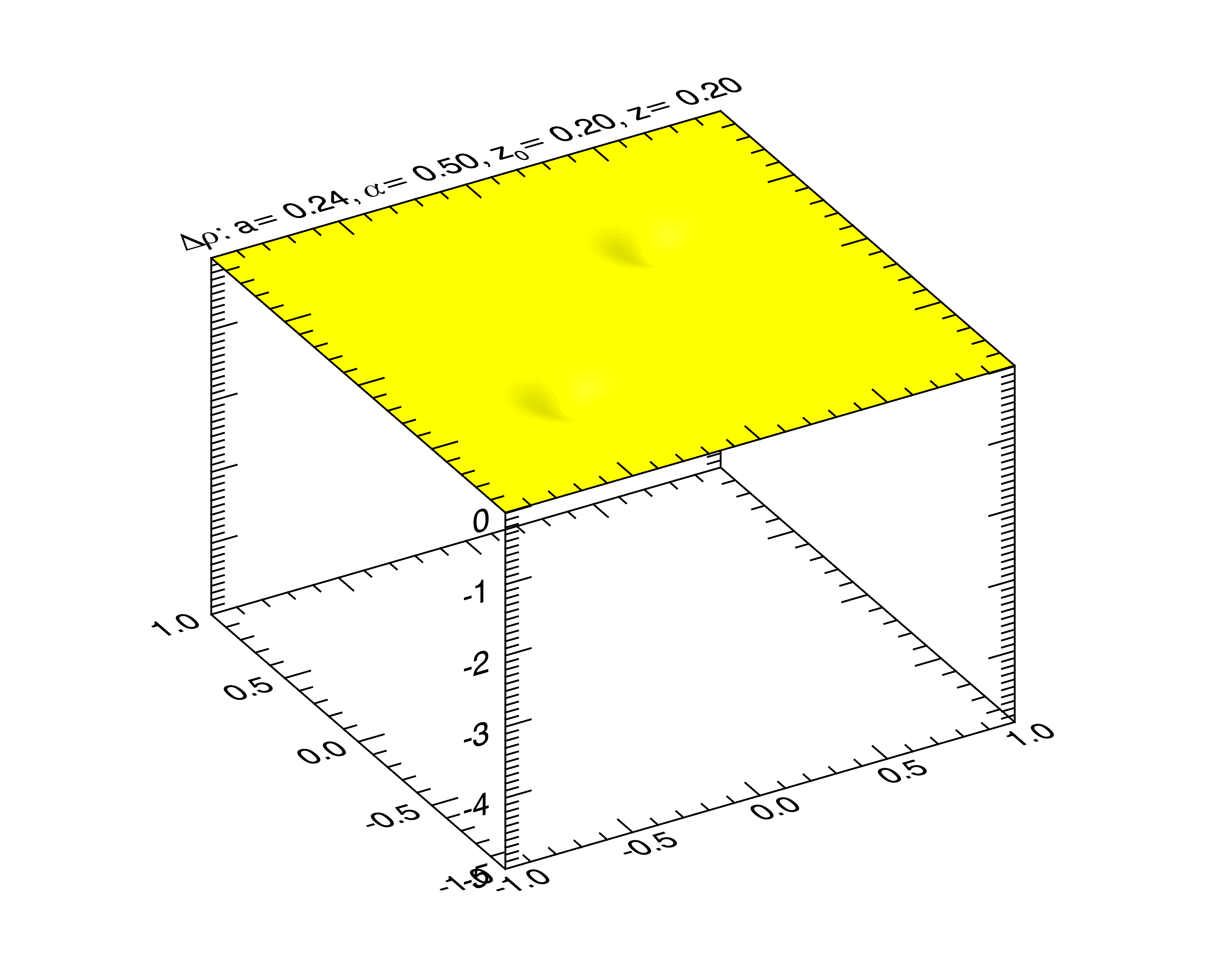
(e)                                      (f)

Figure 8.: Surface plots of $\Delta p$ and $\Delta\rho$ at the heights $z=0$ ((a) and (b)), $z=z_{0}/2$ ((c) and (d))and $z=z_{0}$ ((e) and (f)), showing the variation of pressure and density in the $x$- and $y$-directions. fig:pandrho-surfaces

In Figures fig:pandrho-lineplots and fig:pandrho-surfaces we show the spatial variation of

$$\Delta p=-f(z)\frac{B_{z}^{2}}{2\mu_{0}}\ilabel{eq:def-delp}$$ (30)

and

$$\Delta\rho=\frac{1}{g}\left(\frac{{\mathrm{d}}f}{{\mathrm{d}}z}\frac{B_{z}^{2}}{2\mu_{0}}+\frac{f}{\mu_{0}}{\mathbfit B}\cdot{\bf\nabla}B_{z}\right).\ilabel{eq:def-delrho}$$ (31)

In these two figures $\Delta p$ is normalised by $B_{\mathrm{max}}^{2}/\mu_{0}$, where $B_{\mathrm{max}}$ is the maximum value of $B_{z}$ at $z=0$, and $\Delta\rho$ is normalised by $B_{\mathrm{max}}^{2}/(\mu_{0}gL)$ Figure fig:pandrho-lineplots shows the variation of $\Delta p$ and $\Delta\rho$ with height for $0\leq z\leq 2z_{0}$ at the position of the maximum of $|B_{z}|$ on the lower boundary, i.e. $x=y=\tilde{\mu}_{x1}\approx-0.382$. We have chosen these $x$ and $y$-coordinates because one expects the largest variations of $\Delta p$ and $\Delta\rho$ to happen there. As one can see both $\Delta p$ and $\Delta\rho$ have negative values and they generally increase with $z$ from their lowest value at $z=0$ until approaching zero around $z=z_{0}$, as expected. The increase of the amplitude of $\Delta p$ and $\Delta\rho$ and their slower increase with $z$ with increasing value of $a$ is also obvious. The latter is caused by the Fourier modes, in particular the lowest order mode, to decrease less fast with height when $a$ increases. Although a detailed analysis is a bit more complicated, one can roughly regard the $z$ dependence of each mode as being given by $\exp(-2\gamma z)$ below and $\exp(-2\delta z)$ above $z\approx z_{0}$. As $a\to a_{\mathrm{max}}$ we have $\gamma\to 0$ for the lowest order mode and hence the mode decreases more slowly with $z$.

We also note that $\Delta\rho$ has a local maximum and minimum just below $z_{0}$. This is caused by the $\frac{{\mathrm{d}}f}{{\mathrm{d}}z}$ term in $\Delta\rho$, which is largest at $z_{0}$. This term becomes the larger the sharper the gradient of $f$ at $z=z_{0}$ is made, i.e. the smaller $\Delta z$ becomes (the derivative actually tends to a $\delta$-function in the limit $\Delta z\to 0$ in which case the $\tanh$-function tends to a step function). For this reason one should not attempt to make $\Delta z$ too small.

   

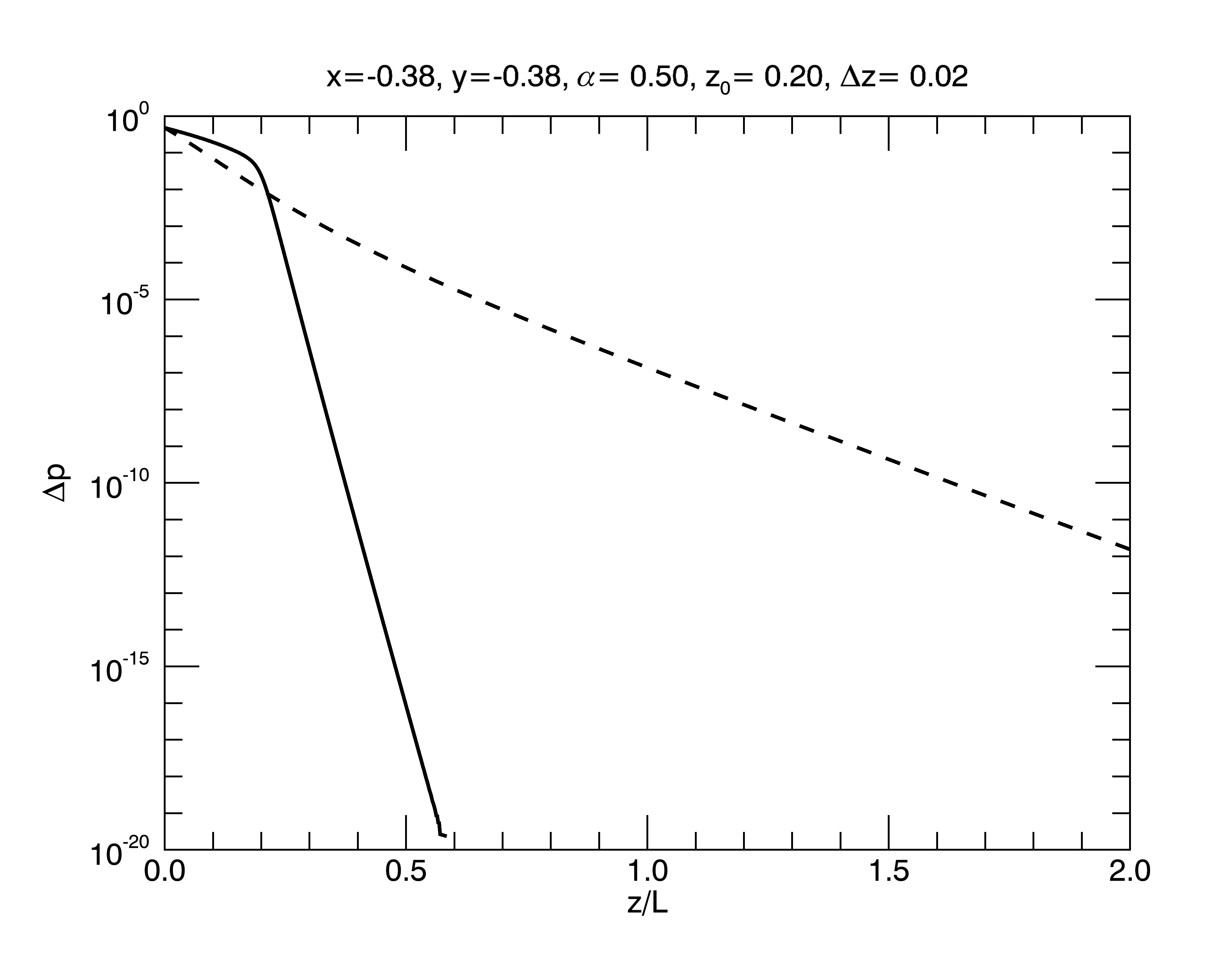
          (a)

   

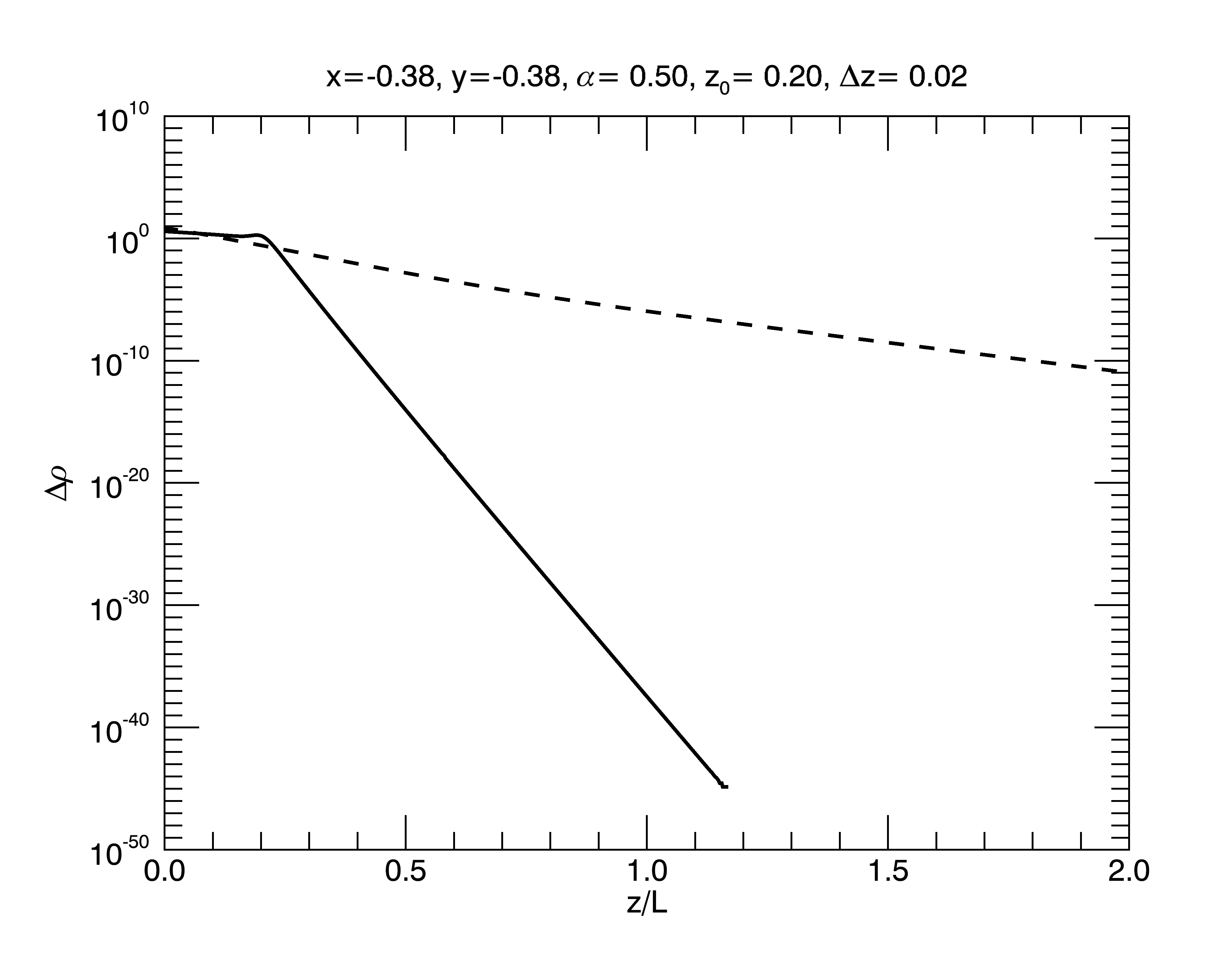
          (b)

Figure 9.: Comparison of the variation with height $z$ of the absolute values of the pressure (panel (a)) and density (panel(b)) deviation from a stratified background atmosphere for the solutions presented in this paper (solid lines) and for a solution with an exponential $f(z)$ (Low, 1991). The plots have a logarithmic $y$-axis to emphasize the difference of the quantities of the solutions, especially the much faster drop-off of the solutions presented in this paper above the transition height $z_{0}$. The parameters chosen for this plot are $\alpha=0.5$, $a=0.48$, $z_{0}/L=0.2$ and $\Delta z=0.1z_{0}$ for the solid line, whereas we have chosen $\bar{a}=0.96$ and $\kappa=1/z_{0}$ (see main text for definitions). The $x$- and $y$-coordinates of these plots are the position of the maximum value of $|B_{z}|$ on the lower boundary, $x/L=\mu_{x}/\pi\approx-0.38$, $y/L=\mu_{y}/\pi\approx-0.38$.fig:pandrho-comparison

To keep the pressure and density positive everywhere we need to make the background pressure $p_{0}(z)$ and the corresponding background density $\rho_{0}(z)=-\frac{1}{g}\frac{{\mathrm{d}}p_{0}}{{\mathrm{d}}z}$ positive and larger at every height $z$ than the minimum values of $\Delta p$ and $\Delta\rho$ for all $x$, $y$ values at the same height (see e.g. Wiegelmann et al., 2015). As one can see from Figures fig:pandrho-lineplots and fig:pandrho-surfaces for this new solution family this condition is only needed to be satisfied for $z<z_{0}$ in the case $b=1.0$ because the contributions to the pressure and the density by $\Delta p$ and $\Delta\rho$ become arbitrarily small very fast for $z>z_{0}$. In Figure fig:pandrho-comparison we show a comparison of variation with $z$ of the absolute values of $\Delta p$ and $\Delta\rho$ (again at $x=y=\tilde{\mu}_{x1}\approx-0.382$), for a solution of the family presented in this paper and a solution for $f(z)=\bar{a}\exp(-\kappa z)$ (Low, 1991). We remark that in order to start with the same pressure at $z=0$ one has to set $\bar{a}=2a$. We have also chosen the inverse length scale $\kappa=1/z_{0}$, corresponding to the height of the transition of the solutions presented in this paper from non-force-free to force-free. These plots clearly show that while for both sets of solutions the pressure and density deviations decrease rapidly for $z>z_{0}$, the decrease is much more rapid for our solutions, which, as already stated above, reduces the need for artificially adjusting the stratified background atmosphere in this region to avoid negative density or pressure values.

One could of course argue that by increasing $\kappa$, i.e. reducing the length scale over which the exponential $f(z)$ and hence the pressure and density deviations decay, one could in principle achieve a similar effect for the exponential $f(z)$. However, for this $f(z)$ this would also decrease the effect of the non-force-free part of the current density in the regions below $z_{0}$ and hence reduce the effect of the non-force-free part of the current density, which somewhat defeats the purpose of using such a magnetic field model for extrapolation in the first place. Because the solutions presented in this paper can guarantee a very rapid transition to a linear force-free magnetic field, but still allow us to control the region $z<z_{0}$ separately this problem does not arise in the new family of solutions.

5 Discussion and Conclusions

sec:discussion

We have presented a new family of three-dimensional MHS solutions based on the general theory originally developed by Low and co-workers (e.g. Low, 1985; Bogdan and Low, 1986; Low, 1991, 1992), although we have used the alternative mathematical formulation by Neukirch and Rastätter (1999). The main motivation for trying to find these solutions was that they are of potential importance for analytical non-force-free magnetic field extrapolation methods. The new family of solutions allows for the MHS nature of the equilibria to be limited to a domain below a specific pre-determined height with a smooth transition to a potential or linear force-free solution possible above height. This is achieved by choosing one of the fundamental free functions of the theory in the form of a hyperbolic tangent. It is important to emphasize that this is just one possibility of choosing the parameters for this equilibrium family and that MHS solutions in the full domain are also possible.

While such a transition is also possible with the free function mentioned above chosen in the form a decaying exponential function (e.g. Low, 1991, 1992; Aulanier et al., 1998, 1999; Wiegelmann et al., 2015, 2017), the new solution family allows much more control over the transition from the MHS domain to the non-MHS domain, in particular regarding the departures of the plasma pressure and density from a stratified atmosphere. This property can be of importance for keeping the plasma pressure and density of the solution positive and should make this equilibrium family interesting for magnetic field extrapolation purposes when a non-force-free layer has to be included. We emphasize that we do not regard these analytical extrapolation methods as replacements for numerical methods for non-force-free magnetic field extrapolation, but as a numerically relatively cheap complementary method, which could be used as an initial ”quick look” tool. Obviously, the limitations that arise from having to make a number of strong assumptions to allow analytical progress have to born in mind when applying these methods.

Appendix A Fourier Decomposition of Example Magnetic Field

app:fourier

Using the identity (e.g. Abramowitz and Stegun, 1965; Olver et al., 2010)

$$\exp[x\cos(y)]=\mbox{I}_{0}(x)+2\sum\limits_{n=1}^{\infty}\mbox{I}_{n}(x)\cos(ny),\ilabel{eq:expcos-in-I}$$ (32)

plus trigonometric identities, it is straightforward (albeit a bit tedious) to write the expression for $B_{z}(x,y,0)$ in Equation eq:magnetogram in the form

$$B_{z}(x,y,0) = \sum\limits_{n=1}^{\infty}\sum\limits_{m=1}^{\infty}[a_{nm}\sin(n\bar{x})\sin(m\bar{y})+b_{nm}\sin(n\bar{x})\cos(m\bar{y})+$$ (33)

$$\mbox{\hskip 42.67912pt}c_{nm}\cos(n\bar{x})\sin(m\bar{y})+d_{nm}\cos(n\bar{x})\cos(m\bar{y})+$$

$$\sum\limits_{n=1}^{\infty}[b_{n0}\sin(n\bar{x})+d_{n0}\cos(n\bar{x})]+$$

$$\sum\limits_{m=1}^{\infty}[c_{0m}\sin(m\bar{y})+d_{0m}\cos(m\bar{y})],$$

with

$$a_{nm} = \frac{B_{0}}{\pi^{2}}\left[I_{f1,nm}\sin(n\bar{\mu}_{x1})\sin(m\bar{\mu}_{y1})-I_{f2,nm}\sin(n\bar{\mu}_{x2})\sin(m\bar{\mu}_{y2})\right],$$ (34)

$$b_{nm} = \frac{B_{0}}{\pi^{2}}\left[I_{f1,nm}\sin(n\bar{\mu}_{x1})\cos(m\bar{\mu}_{y1})-I_{f2,nm}\sin(n\bar{\mu}_{x2})\cos(m\bar{\mu}_{y2})\right],$$ (35)

$$c_{nm} = \frac{B_{0}}{\pi^{2}}\left[I_{f1,nm}\cos(n\bar{\mu}_{x1})\sin(m\bar{\mu}_{y1})-I_{f2,nm}\cos(n\bar{\mu}_{x2})\sin(m\bar{\mu}_{y2})\right],$$ (36)

$$d_{nm} = \frac{B_{0}}{\pi^{2}}\left[I_{f1,nm}\cos(n\bar{\mu}_{x1})\cos(m\bar{\mu}_{y1})-I_{f2,nm}\cos(n\bar{\mu}_{x2})\cos(m\bar{\mu}_{y2})\right],$$ (37)

where the factors $I_{fi,nm}$ are defined as

$$I_{fi,nm}=\frac{\mbox{I}_{n}(\tilde{\kappa}_{xi})\mbox{I}_{m}(\tilde{\kappa}_{yi})}{2\mbox{I}_{0}(\tilde{\kappa}_{xi})\mbox{I}_{0}(\tilde{\kappa}_{yi})}\times\left\{\begin{array}[]{ll}1&\mbox{for $m=0$, $n>0$ or $n=0$, $m>0$ }\\ 2&\mbox{for $m>0$ and $n>0$}\end{array}\right..\ilabel{eq:I-f-def}$$ (38)

The corresponding series for $B_{z}$ is given by

$$B_{z}(x,y,0) = \sum\limits_{n=1}^{\infty}\sum\limits_{m=1}^{\infty}k_{nm}^{2}\bar{\Phi}_{nm}(0)[\bar{a}_{nm}\sin(n\bar{x})\sin(m\bar{y})+\bar{b}_{nm}\sin(n\bar{x})\cos(m\bar{y})+$$ (39)

$$\mbox{\hskip 42.67912pt}\bar{c}_{nm}\cos(n\bar{x})\sin(m\bar{y})+\bar{d}_{nm}\cos(n\bar{x})\cos(m\bar{y})]+$$

$$\sum\limits_{n=1}^{\infty}k_{n0}^{2}\bar{\Phi}_{nm}(0)[\bar{b}_{n0}\sin(n\bar{x})+\bar{d}_{n0}\cos(n\bar{x})]+$$

$$\sum\limits_{m=1}^{\infty}k_{0m}^{2}\bar{\Phi}_{nm}(0)[\bar{c}_{0m}\sin(m\bar{y})+\bar{d}_{0m}\cos(m\bar{y})],$$

with $\bar{\Phi}_{nm}(z)$ the solution of Equation eq:Phibar-eckart-equation for the wave vector

$$k^{2}_{nm}=\frac{\pi^{2}}{L^{2}}(n^{2}+m^{2}).$$ (40)

We remark that $n$ or $m$ are allowed to take on the value $0$, but not both at the same time. Comparing Equations eq:Bz_fourierexp and eq:Bz_fourierexp-sol one can easily see that $\bar{a}_{nm}=a_{nm}/(k_{nm}^{2}\bar{\Phi}_{nm}(0))$ etc.

Acknowledgments

For producing some of the figures in this paper the authors have used of the IDL routines for hypergeometric functions by Michele Cappellari (https://github.com/surftour/astrotools/blob/master/idlstuff/IDL_kin/jam_modelling/utils/hypergeometric2f1.pro and
http://www-astro.physics.ox.ac.uk/m̃xc/software/). TN acknowledges financial support by the UK’s Science and Technology Facilities Council (STFC), Consolidated Grants ST/K000950/1, ST/N000609/1 and ST/S000402/1 and would like to thank the colleagues at the Max-Planck-Institute for Solar System Research for their hospitality during his visits in 2014 and 2015 when the idea for this research originated. TW acknowledges financial support by DFG Grant WI 3211/4-1.

Disclosure of Potential Conflicts of Interest

The authors declare that they have no conflicts of interest.

References

- Abramowitz and Stegun (1965) Abramowitz, M., Stegun, I.A.: 1965, Handbook of Mathematical Functions, Dover Publications, New York.
- Al-Salti and Neukirch (2010) Al-Salti, N., Neukirch, T.: 2010, Three-dimensional solutions of the magnetohydrostatic equations: Rigidly rotating magnetized coronae in spherical geometry. A&A 520, A75. DOI. ADS.
- Al-Salti, Neukirch, and Ryan (2010) Al-Salti, N., Neukirch, T., Ryan, R.: 2010, Three-dimensional solutions of the magnetohydrostatic equations: rigidly rotating magnetized coronae in cylindrical geometry. A&A 514, A38. DOI. ADS.
- Alissandrakis (1981) Alissandrakis, C.E.: 1981, On the computation of constant alpha force-free magnetic field. A&A 100, 197. ADS.
- Aulanier et al. (1998) Aulanier, G., Démoulin, P., Schmieder, B., Fang, C., Tang, Y.H.: 1998, Magnetohydrostatic model of a bald-patch flare. Sol. Phys. 183, 369.
- Aulanier et al. (1999) Aulanier, G., Démoulin, P., Mein, N., Van Driel-Gesztelyi, L., Mein, P., Schmieder, B.: 1999, 3-D magnetic configurations supporting prominences. III. Evolution of fine structures observed in a filament channel. A&A 342, 867.
- Bagenal and Gibson (1991) Bagenal, F., Gibson, S.: 1991, Modeling the large-scale structure of the solar corona. J. Geophys. Res. 96, 17663. DOI. ADS.
- Bogdan and Low (1986) Bogdan, T.J., Low, B.C.: 1986, The three-dimensional structure of magnetostatic atmospheres. II - Modeling the large-scale corona. ApJ 306, 271.
- Chiu and Hilton (1977) Chiu, Y.T., Hilton, H.H.: 1977, Exact Green’s function method of solar force-free magnetic-field computations with constant alpha. I - Theory and basic test cases. ApJ 212, 873.
- De Rosa et al. (2009) De Rosa, M.L., Schrijver, C.J., Barnes, G., Leka, K.D., Lites, B.W., Aschwanden, M.J., Amari, T., Canou, A., McTiernan, J.M., Régnier, S., Thalmann, J.K., Valori, G., Wheatland, M.S., Wiegelmann, T., Cheung, M.C.M., Conlon, P.A., Fuhrmann, M., Inhester, B., Tadesse, T.: 2009, A Critical Assessment of Nonlinear Force-Free Field Modeling of the Solar Corona for Active Region 10953. ApJ 696, 1780. DOI. ADS.
- (11) NIST Digital Library of Mathematical Functions, http://dlmf.nist.gov/, Release 1.0.9 of 2014-08-29. Online companion to Olver et al. (2010). http://dlmf.nist.gov/.
- Gent, Fedun, and Erdélyi (2014) Gent, F.A., Fedun, V., Erdélyi, R.: 2014, Magnetohydrostatic Equilibrium. II. Three-dimensional Multiple Open Magnetic Flux Tubes in the Stratified Solar Atmosphere. ApJ 789, 42.
- Gent et al. (2013) Gent, F.A., Fedun, V., Mumford, S.J., Erdélyi, R.: 2013, Magnetohydrostatic equilibrium - I. Three-dimensional open magnetic flux tube in the stratified solar atmosphere. MNRAS 435, 689.
- Gibson and Bagenal (1995) Gibson, S.E., Bagenal, F.: 1995, Large-scale magnetic field and density distribution in the solar minimum corona. J. Geophys. Res. 100, 19865. DOI. ADS.
- Gibson, Bagenal, and Low (1996) Gibson, S.E., Bagenal, F., Low, B.C.: 1996, Current sheets in the solar minimum corona. J. Geophys. Res. 101, 4813. DOI. ADS.
- Gilchrist and Wheatland (2013) Gilchrist, S.A., Wheatland, M.S.: 2013, A Magnetostatic Grad-Rubin Code for Coronal Magnetic Field Extrapolations. Sol. Phys. 282, 283. DOI. ADS.
- Harvey (2012) Harvey, J.W.: 2012, Chromospheric Magnetic Field Measurements in a Flare and an Active Region Filament. Sol. Phys. 280, 69. DOI. ADS.
- Lagg et al. (2017) Lagg, A., Lites, B., Harvey, J., Gosain, S., Centeno, R.: 2017, Measurements of Photospheric and Chromospheric Magnetic Fields. Space Sci. Rev. 210, 37. DOI. ADS.
- Lanza (2008) Lanza, A.F.: 2008, Hot Jupiters and stellar magnetic activity. A&A 487, 1163. DOI. ADS.
- Lanza (2009) Lanza, A.F.: 2009, Stellar coronal magnetic fields and star-planet interaction. A&A 505, 339. DOI. ADS.
- Low (1982) Low, B.C.: 1982, Magnetostatic atmospheres with variations in three dimensions. ApJ 263, 952.
- Low (1984) Low, B.C.: 1984, Three-dimensional magnetostatic atmospheres - Magnetic field with vertically oriented tension force. ApJ 277, 415.
- Low (1985) Low, B.C.: 1985, Three-dimensional structures of magnetostatic atmospheres. I - Theory. ApJ 293, 31.
- Low (1991) Low, B.C.: 1991, Three-dimensional structures of magnetostatic atmospheres. III - A general formulation. ApJ 370, 427.
- Low (1992) Low, B.C.: 1992, Three-dimensional structures of magnetostatic atmospheres. IV - Magnetic structures over a solar active region. ApJ 399, 300.
- Low (1993a) Low, B.C.: 1993a, Three-dimensional structures of magnetostatic atmospheres. V - Coupled electric current systems. ApJ 408, 689.
- Low (1993b) Low, B.C.: 1993b, Three-dimensional structures of magnetostatic atmospheres. VI - Examples of coupled electric current systems. ApJ 408, 693.
- Low (2005) Low, B.C.: 2005, Three-dimensional Structures of Magnetostatic Atmospheres. VII. Magnetic Flux Surfaces and Boundary Conditions. ApJ 625, 451. DOI. ADS.
- MacTaggart et al. (2016) MacTaggart, D., Gregory, S.G., Neukirch, T., Donati, J.-F.: 2016, Magnetohydrostatic modelling of stellar coronae. MNRAS 456, 767. DOI. ADS.
- Mardia and Jupp (1999) Mardia, K., Jupp, P.E.: 1999, Directional Statistics, Wiley, Chichester, England.
- Metcalf et al. (1995) Metcalf, T.R., Jiao, L., McClymont, A.N., Canfield, R.C., Uitenbroek, H.: 1995, Is the Solar Chromospheric Magnetic Field Force-free? ApJ 439, 474. DOI. ADS.
- Nakagawa and Raadu (1972) Nakagawa, Y., Raadu, M.A.: 1972, On Practical Representation of Magnetic Field. Sol. Phys. 25, 127. DOI. ADS.
- Neukirch (1995) Neukirch, T.: 1995, On self-consistent three-dimensional solutions of the magnetohydrostatic equations. A&A 301, 628.
- Neukirch (1997a) Neukirch, T.: 1997a, 3D solar magnetohydrostatic structures. Phys. Chem. Earth 22, 405.
- Neukirch (1997b) Neukirch, T.: 1997b, Nonlinear self-consistent three-dimensional arcade-like solutions of the magnetohydrostatic equations. A&A 325, 847.
- Neukirch (2009) Neukirch, T.: 2009, Three-dimensional analytical magnetohydrostatic equilibria of rigidly rotating magnetospheres in cylindrical geometry. Geophys. Astrophys. Fluid Dyn. 103, 535. DOI. ADS.
- Neukirch and Rastätter (1999) Neukirch, T., Rastätter, L.: 1999, A new method for calculating a special class of self-consistent three-dimensional magnetoshydrostatic equilibria. A&A 348, 1000.
- Olver et al. (2010) Olver, F.W.J., Lozier, D.W., Boisvert, R.F., Clark, C.W. (eds.): 2010, NIST Handbook of Mathematical Functions, Cambridge University Press, New York, NY. Print companion to NIST Digital Library of Mathematical Functions.
- Osherovich (1985a) Osherovich, V.A.: 1985a, The eigenvalue approach in modelling solar magnetic structures. Aust. J. Phys. 38, 975.
- Osherovich (1985b) Osherovich, V.A.: 1985b, Quasi-potential magnetic fields in stellar atmospheres. I - Static model of magnetic granulation. ApJ 298, 235.
- Otto, Büchner, and Nikutowski (2007) Otto, A., Büchner, J., Nikutowski, B.: 2007, Force-free magnetic field extrapolation for MHD boundary conditions in simulations of the solar atmosphere. A&A 468, 313. DOI. ADS.
- Petrie (2000) Petrie, G.J.D.: 2000, Three-dimensional Equilibrium Solutions to the Magnetohydrodynamic Equations and their Application to Solar Coronal Structures. PhD thesis, School of Mathematics and Statistics, University of St. Andrews, North Haugh, St Andrews KY16 9SS. ADS.
- Petrie and Lothian (2003) Petrie, G.J.D., Lothian, R.M.: 2003, An investigation of the topology and structure of constant-alpha force-free fields. A&A 398, 287. DOI. ADS.
- Petrie and Neukirch (2000) Petrie, G.J.D., Neukirch, T.: 2000, The Green’s function method for non-force-free three-dimensional solutions of the magnetohydrostatic equations. A&A 356, 735.
- Priest (2014) Priest, E.R.: 2014, Magnetohydrodynamics of the Sun, Cambridge University Press, Cambridge, UK.
- Régnier (2013) Régnier, S.: 2013, Magnetic Field Extrapolations into the Corona: Success and Future Improvements. Sol. Phys. 288, 481. DOI. ADS.
- Ruan et al. (2008) Ruan, P., Wiegelmann, T., Inhester, B., Neukirch, T., Solanki, S.K., Feng, L.: 2008, A first step in reconstructing the solar corona self-consistently with a magnetohydrostatic model during solar activity minimum. A&A 481, 827. DOI. ADS.
- Seehafer (1978) Seehafer, N.: 1978, Determination of constant alpha force-free solar magnetic fields from magnetograph data. Sol. Phys. 58, 215. DOI. ADS.
- Wheatland (1999) Wheatland, M.S.: 1999, A Better Linear Force-free Field. ApJ 518, 948. DOI. ADS.
- Wiegelmann and Neukirch (2006) Wiegelmann, T., Neukirch, T.: 2006, An optimization principle for the computation of MHD equilibria in the solar corona. A&A 457, 1053. DOI. ADS.
- Wiegelmann and Sakurai (2012) Wiegelmann, T., Sakurai, T.: 2012, Solar Force-free Magnetic Fields. Living Rev. Sol. Phys. 9, 5. DOI. ADS.
- Wiegelmann, Thalmann, and Solanki (2014) Wiegelmann, T., Thalmann, J.K., Solanki, S.K.: 2014, The magnetic field in the solar atmosphere. A&A Rev. 22, 78. DOI. ADS.
- Wiegelmann et al. (2015) Wiegelmann, T., Neukirch, T., Nickeler, D.H., Solanki, S.K., Martínez Pillet, V., Borrero, J.M.: 2015, Magneto-static Modeling of the Mixed Plasma Beta Solar Atmosphere Based on Sunrise/IMaX Data. ApJ 815, 10. DOI. ADS.
- Wiegelmann et al. (2017) Wiegelmann, T., Neukirch, T., Nickeler, D.H., Solanki, S.K., Barthol, P., Gandorfer, A., Gizon, L., Hirzberger, J., Riethmüller, T.L., van Noort, M., Blanco Rodríguez, J., Del Toro Iniesta, J.C., Orozco Suárez, D., Schmidt, W., Martínez Pillet, V., Knölker, M.: 2017, Magneto-static Modeling from Sunrise/IMaX: Application to an Active Region Observed with Sunrise II. ApJS 229, 18. DOI. ADS.
- Wilson and Neukirch (2018) Wilson, F., Neukirch, T.: 2018, Three-dimensional solutions of the magnetohydrostatic equations for rigidly rotating magnetospheres in cylindrical coordinates. Geophys. Astrophys. Fluid Dyn. 112, 74. DOI. ADS.
- Zhao and Hoeksema (1993) Zhao, X., Hoeksema, J.T.: 1993, Unique determination of model coronal magnetic fields using photospheric observations. Sol. Phys. 143, 41. ADS.
- Zhao and Hoeksema (1994) Zhao, X., Hoeksema, J.T.: 1994, A coronal magnetic field model with horizontal volume and sheet currents. Sol. Phys. 151, 91. ADS.
- Zhao, Hoeksema, and Scherrer (2000) Zhao, X.P., Hoeksema, J.T., Scherrer, P.H.: 2000, Modeling the 1994 April 14 Polar Crown SXR Arcade Using Three-Dimensional Magnetohydrostatic Equilibrium Solutions. ApJ 538, 932. DOI. ADS.
- Zhu and Wiegelmann (2018) Zhu, X., Wiegelmann, T.: 2018, On the Extrapolation of Magnetohydrostatic Equilibria on the Sun. ApJ 866, 130. DOI. ADS.