A New Distribution-Free Concept for Representing, Comparing, and Propagating Uncertainty in Dynamical Systems with Kernel Probabilistic Programming

Abstract

This work presents the concept of kernel mean embedding and kernel probabilistic programming in the context of stochastic systems. We propose formulations to represent, compare, and propagate uncertainties for fairly general stochastic dynamics in a distribution-free manner. The new tools enjoy sound theory rooted in functional analysis and wide applicability as demonstrated in distinct numerical examples. The implication of this new concept is a new mode of thinking about the statistical nature of uncertainty in dynamical systems.

AND

1 Introduction

Classic stochastic control methods such as LQG hinge on the mathematical fact that the family of Gaussian distributions is closed under an affine transformation. This allows uncertainty to be propagated in a tractable manner under the Gaussianity assumption. Robust control methods, such as the classic tube model predictive control, also rely on the linearity of dynamics to propagate the polytopic uncertainty. However, when we move beyond those assumptions to the territories of nonlinear dynamics and non-Gaussian noise, uncertainty propagation becomes difficult or even intractable.

A central component in robust and stochastic control is how to represent the system uncertainty. To this end, point estimate, ellipsoidal uncertainty set, Gaussian distribution, or randomized computer simulations have been used in various applications. Along with those, a few families of uncertainty propagation methods have been proposed, e.g., generalized polynomial chaos approximation, Gaussian processes. The representation and propagation affect control as well as system identification. For example, a parameter estimation problem typically uses the likelihood function as its criterion for goodness-of-fit, which requires assuming the distribution family.

Consider an illustrative sketch in Figure 1. How can we measure the differences between system models? If the dynamical system of interest is deterministic (left), then we can simply compare the solutions of the systems in the sense of Euclidean distance.

Figure 1: An illustrative example of deterministic (left) and stochastic (right) dynamical systems. Notice the system in (right, red) is stochastic and bi-modal.

Now we consider Figure 1 (right), which illustrates the evolution of two stochastic dynamical systems (with arbitrary distribution). Due to the stochasticity, the solutions are distributions. Comparison in Euclidean distance is no longer feasible. How do we incorporate statistical information without imposing strong distributional assumptions? The question we address is how to represent, compare, and propagate the randomness in dynamical systems in a quantitative way.

This work proposes to embed uncertain state distributions into the reproducing kernel Hilbert spaces (RKHS), enabling quantification and algebraic operations therein. The main contributions of this work are the following.

• We introduce the RKHS embedding method of kernel probabilistic programming in the context of uncertain dynamical systems. The resulting formulations of representation, comparison, and propagation methods are our main contributions.

• Through distinct numerical examples, we demonstrate the flexible and distribution-free nature of our method as a unifying tool for dynamical systems.

• We propose a recursive reduced set method to propagate the system uncertainty by iteratively solving an optimization problem. This forms fixed-size kernel expansions rather than allowing the number of uncertainty realizations to explode over time.

1.0.1 Notation:

In this work, the state of uncertain dynamical systems are denoted by $x(\tau,\xi)$, where $\tau$ is time and $\xi$ is the uncertainty in the system, e.g., a disturbance process. The Stieltjes integral $\int\cdot\ dP$ denotes the integration w.r.t. either a continuous or a discrete probability measure $P$. Symbol $\mathcal{X}$ often denotes a nonempty set and $\mathcal{H}$ a reproducing kernel Hilbert space (RKHS). We write $\xi\sim P$ to denote that the random variable (RV) $\xi$ follows the distribution law $P$.

2 Background & related work

2.1 Uncertainty quantification in dynamical systems

Stochastic dynamical system refers to a system whose evolution is affected by non-deterministic disturbances. To illustrate our idea concretely, let us consider a simple example of stochastic ODE that was studied in Xiu and Karniadakis (2002):

$$\dot{x}(t)=\xi\ x,\quad x(0)=x_{0},$$ (1)

where the parameter $\xi$ is uncertain. This uncertainty may enter as (a) time-invariant, or, more generally (b) time-varying stochastic process. For a moment, let us consider case (a) and the parameter follows a certain distribution law $\xi\sim P_{\xi}$. This is hence an initial value problem (IVP) with uncertain parameter. The problem of quantifying the distribution of the solution $x(t,\xi)$ to the IVP (1) is typically referred to as the uncertainty quantification in dynamical systems.

One somewhat trivial approach of quantifying the solution is the Monte Carlo sampling that samples $\{\xi^{1},\xi^{2},\dots,\xi^{N}\}$ from the underlying distribution. Then we deterministically integrate the ODE with those realizations of the uncertain parameter to obtain solutions $\{x(t,\xi^{i})\}_{i=1}^{N},\ \forall t$. We may later extract the moment statistics of $x(t,\xi)$ by its Monte Carlo estimation.

In numerical analysis, one representative thread of works in uncertainty quantification is the generalized polynomial chaos (gPC) method. It expands the solution of IVP (1) as a series in orthogonal polynomial basis functions $\{\phi_{i}(\xi)\}_{i=1}^{N}$,

$$x(t,\xi)=\sum_{i=1}^{\infty}\alpha_{i}\phi_{i}(\xi).$$

This expansion is mathematically elegant in that the basis $\phi_{i}(\xi)$’s account for the stochasticity and the expansion coefficients $\alpha_{i}$’s are deterministic. From this point onward, we can either follow Galerkin’s method propagate the coefficients $\alpha_{i}$ through the dynamical systems as in Xiu and Karniadakis (2002), or, use the so-called stochastic collocation to numerically integrate the IVP (1) at certain collocation nodes $\{\xi^{1},\xi^{2},\dots,\xi^{N}\}$ as in Xiu (2009).

Another well-developed methodology in Bayesian statistics is the Gaussian process (GP). Intuitively, GP generalizes the Gaussian distribution to the distribution of functions. For example, dynamics described by a difference equation can be modeled by a GP prior, i.e., $x_{t+1}-x_{t}=f(x_{t})\sim\mathcal{GP}(\mu(x_{t}),\sigma(x_{t}))$ where $x_{t}$ is a shorthand for $x(t,\xi)$. Given data samples, it can be shown that the posterior predictive distribution for an unseen state is also Gaussian. This allows us to quantify the distribution of solution $x(t,\xi)$. We refer to Rasmussen and Williams (2006) for an accessible introduction.

Mathematically speaking, gPC and GP are both surrogate function classes enabled by function approximation theory. This paper does not focus on analyzing the function approximation aspect. Instead, the embedding method we shall propose in Section 3 calls for a shift in our ways of thinking about statistical distributions.

2.2 Goodness-of-fit measure for system identification

System identification studies how to construct mathematical models of dynamical systems from observed data. While this paper does not directly propose a system identification algorithm, we show how the proposed concept can impact how we analyze and compare the models in terms of goodness-of-fit. To give readers a concrete example of this new concept, we revisit the parameter and variability estimation (PVE) proposed by Mohammadi et al. (2015) in Section 4.2. This may be thought of as an alternative to the least square (LSQ) estimation, whose underlying assumption is that the system is following an additive Gaussian distribution with fixed variance, $y=f(x)+\xi,\ \xi\sim N(\bar{\xi}_{\mathrm{LSQ}},\sigma_{\mathrm{LSQ}}).$ In contrast, PVE is based on the robust optimization idea that the disturbance should lie within an ellipsoidal uncertainty set $\xi\in\mathcal{E}(\bar{\xi}_{\mathrm{PVE}},Z_{\mathrm{PVE}})$ but not making any assumptions on the distribution family. The PVE method then formulates the identification of the uncertain ellipsoid as a semidefinite programming (SDP) problem. More details are provided in that paper.

It can be relatively difficult to compare an LSQ point estimate (or MLE in general) with e.g. PVE because they do not share the same likelihood . This paper proposes such a unifying framework of comparing different system models’ goodness-of-fit.

2.3 Reproducing kernel Hilbert space (RKHS) embedding

A kernel is a real-valued bivariate function $k(\cdot,\cdot):\mathcal{X}\times\mathcal{X}\to\mathbb{R}$. It is said to be positive definite if $\sum_{i,j=1}^{n}\alpha_{i}\alpha_{j}k(x_{i},x_{j})\geq 0$ for any $n\in\mathbb{N}$, $(\alpha_{1},\ldots,\alpha_{n})\in\mathbb{R}^{n}$, and $(x_{1},\ldots,x_{n})\in\mathcal{X}^{n}$. In addition, it is a reproducing kernel of an RKHS $\mathcal{H}$ if (i) $\forall x\in\mathcal{X}$, $k(x,\cdot)\in\mathcal{H}$ and (ii) $\forall x\in\mathcal{X},f\in\mathcal{H}$, $f(x)=\langle f,k(x,\cdot)\rangle_{\mathcal{H}}$. The latter is known as the reproducing property of $\mathcal{H}$. Choosing $f=k(x^{\prime},\cdot)$ for some $x^{\prime}\in\mathcal{X}$ and applying the reproducing property yield the kernel trick

$$k(x,x^{\prime})=\langle k(x,\cdot),k(x^{\prime},\cdot)\rangle_{\mathcal{H}}=\langle\phi(x),\phi(x^{\prime})\rangle_{\mathcal{H}}.$$ (2)

That is, we can view the kernel evaluation $k(x,x^{\prime})$ as a generalized similarity measure between $x$ and $x^{\prime}$ after mapping them into the feature space $\mathcal{H}$. We refer to $\phi$ defined above as a canonical feature map associated with the kernel $k$. One of the most common kernels on $\mathbb{R}^{d}$ is the Gaussian kernel

$$k(x,x^{\prime})=\exp\left(-\frac{1}{2\sigma^{2}}\|x-x^{\prime}\|_{2}^{2}\right),\quad x,x^{\prime}\in\mathbb{R}^{d},$$ (3)

where $\sigma>0$ is a bandwidth parameter.

An important application of kernel methods is in representing probability measures via kernel mean embedding (KME) [Smola et al. (2007)]. This line of work can be thought of as a systematic way of endowing unstructured data with representations in a Hilbert space to provide the ability to perform algebraic operations therein. Mathematically, we define the KME of a random variable $X$ as follows.

Definition 2.1

(Kernel mean embedding) Given random variable $X\sim P$ and kernel $k$ for which $\mathbb{E}_{X}\sqrt{k(X,X)}<\infty$, we define the kernel mean embedding of $X$ as a function

$$\mu^{k}_{X}(\cdot)=\int k(x,\cdot)\ dP(x).$$

This function is a member of the RKHS, $\mu^{k}_{X}\in\mathcal{H}$ associated with the kernel $k$.

In the rest of the paper, we follow the convention in kernel machine learning to simply write the function $\mu^{k}_{X}(\cdot)$ as $\mu_{X}$ to emphasize that it is an element of the RKHS $\mathcal{H}$. It has been shown that if $k$ belongs to a class of kernels known as characteristic kernels, then $\mu_{X}$ uniquely determines the distribution $P$; see, e.g., Fukumizu et al. (2004); Sriperumbudur et al. (2010).

To help readers get a concrete understanding, we outline common kernels and the information their KME preserve in Table 1. We then give examples of the explicit forms of the KMEs.

Table 1: Common kernels and what statistical information their KME preserve. More examples can be found in Muandet et al. (2017)

Linear	$k(x,x^{\prime})=x^{\top}x^{\prime}$	Mean of distribution
Polynomial	$k(x,x^{\prime})=(x^{\top}x^{\prime}+1)^{p}$	Up to $p$-th moments
Gaussian	$k(x,x^{\prime})=\exp\left(-\frac{\|x-x^{\prime}\|_{2}^{2}}{2\sigma^{2}}\right)$	All information
Exponential	$k(x,x^{\prime})=\exp(x^{\top}x^{\prime})$	All information

2.3.1 Example (Second-order polynomial kernel embedding)

Suppose the kernel function in question is the polynomial kernel of order two $k(x,x^{\prime})=(x^{\top}x^{\prime}+1)^{2}$, the KME is given by

$$\begin{array}[]{ll}\mu_{X}&=\int k(x,\cdot)dP(x)=\int\left(x^{\top}(\cdot)+1\right)^{2}\ dP(x)\\ &=(\cdot)^{\top}\mathbb{E}{xx^{\top}}(\cdot)+2\mathbb{E}{x}^{\top}(\cdot)+1.\end{array}$$ (4)

This shows that the RKHS associated with this KME consists of quadratic functions whose coefficients preserve statistical information up to the second order (mean and variance), but not higher. In general, $p$-th order polynomial kernel embeddings preserve information up to the $p$-th order. A richer kernel embedding, e.g. Gaussian kernel embedding, may preserve information up to infinite order.

Remark Readers familiar with polynomial approximation may recognize that the integrand in (4) can be expanded in certain Wiener-Askey polynomial bases. However, our method differs from the philosophy of gPC expansion in that it does not seek to use finite-order truncation for approximating functions. Rather, we make use of the kernel trick (2) to represent similarity in data even in infinite-dimensional feature space. This gives rise to the power of kernel machine learning.

2.3.2 Example (Exponential kernel embedding)

Given the exponential kernel $k(x,x^{\prime})=e^{\langle x,x^{\prime}\rangle}$, the KME is

$$\mu_{X}=\int e^{\langle x,\cdot\rangle}dP(x).$$

This is the moment-generating function. Notably, replacing $x$ by $-x$ yields the Laplace transform.

The following result in Song (2008) gives the consistency of a sample-based estimator $\hat{\mu}_{X}$ for $\mu_{X}$.

Lemma 2.1

(Smola et al. (2007); Song (2008); estimator for KME) Let us denote by $X$ a random variable and $\{x^{i}\}_{i=1}^{N}$ its i.i.d samples. Then,

$$\hat{\mu}_{X}:=\frac{1}{N}\sum_{i=1}^{N}k(x^{i},\cdot)\to\mu_{X}$$ (5)

as $N\to\infty$ with probability $1$.

Furthermore, Schölkopf et al. (2015); Simon-Gabriel et al. (2016) proved the estimation consistency for KME of transformations of RVs in more general conditions. They term their approach kernel probabilistic programming (KPP).

Lemma 2.2

(KME consistency) Suppose $f:\mathcal{X}\to\mathcal{Z}$ is a continuous function, $k_{x},k_{z}$ are continuous kernels on $\mathcal{X}$ and $\mathcal{Z}$. Under mild conditions [cf. Theorem 1 of Simon-Gabriel et al. (2016)] , the following is true.

$$\text{If }\hat{\mu}^{k_{x}}_{X}\to\mu^{k_{x}}_{X},\text{ then }\hat{\mu}^{k_{z}}_{f(X)}\to\mu^{k_{z}}_{f(X)}.$$

Notably, we do not require samples to be i.i.d. This result equips us with algebraic tools to learn an embedding of $f(X)$ directly from that of $X$. In the rest of the paper, by KPP we mean the RKHS embedding method that performs algebraic operations on KMEs via transformations of random samples.

In the context of reinforcement learning, e.g., in Nishiyama et al. (2012); Grünewälder et al. (2012); Boots et al. (2013), RKHS embeddings of conditional distributions, which is different from ours, were used to learn dynamics. We share the common thread of using RKHS embeddings while differ in a few important aspects, e.g., our use of KPP, numerical integration for continuous-time systems. See Song et al. (2013) for more details and references.

3 Approach

3.1 Representing uncertainty with RKHS embeddings

KPP introduced in the last section gives us a powerful tool to represent distributions without any parametric assumption. In the context of dynamical systems, if we view the evolution of the system uncertainty as transformations of random variables (RV), then KPP naturally becomes a tool to propagate system uncertainty. An important motivation of our methodology is that it shall be distribution-free, i.e., it shall not impose assumptions on the uncertainty distributions (e.g., Gaussianity).

In a nutshell, we represent the distribution of $x(\tau,\xi)$, the state of the dynamical systems (continuous or discrete time), by its KME and the corresponding sample-based estimator given by

$$\begin{array}[]{cc}\mu_{x(\tau,\xi)}=\int k({x(\tau,\xi)},\cdot)dP(\xi),\\ \hat{\mu}_{x(\tau,\xi)}=\sum_{i=1}^{N}\alpha_{i}k({x(\tau,\xi^{i})},\cdot),\end{array}$$ (6)

where a simple choice is $\alpha_{i}=\frac{1}{N}$. As discussed in Section 2.3, KME with second-order polynomial kernel preserves (nominal state) and second (variance) order information commonly used in stochastic control. In this light, we may view our method as a generalization of Monte Carlo moment estimation.

3.2 Goodness-of-fit measure for uncertain system models

As suggested in Figure 1 (right), it may be difficult to quantitatively compare stochastic system models directly. For example, say we have identified an LSQ point estimate $\hat{\xi}_{1}$ and another estimation described by a distribution in uncertain parameter $\hat{\xi}_{2}\sim P_{2}$ based on two different system identification methods. We cannot simply compare the goodness-of-fit by comparing the likelihood objectives as they might differ for different identification methods. Furthermore, the parameter descriptions may also differ (e.g. point estimation vs. set description) In addition, can we be certain, in a quantitative manner, that the systems behave differently after the propagation through dynamics?

We summon the strength of KME to endow almost arbitrary data types the meaning of distance through the Hilbert space embedding. This allows us to compare systems by performing statistical two-sample tests [cf. Gretton et al. (2012)] using the simulation samples.

Given the state distribution embeddings of two different systems $\mu_{x_{t}},\mu_{y_{t}}$ computed as in (6), we may measure how different two stochastic systems are by straightforwardly computing their distance in the embedding Hilbert space, $\|\mu_{x_{t}}-\mu_{y_{t}}\|_{\mathcal{H}}.$ This quantity is also known as a maximum mean discrepancy (MMD). Using kernel trick (2) and the estimator in (6), we obtain the following.

Lemma 3.1

(Sample-based estimator for RKHS distance; MMD) Given two sets of samples $\{x_{i}\}_{i=1}^{M}$ and $\{y_{i}\}_{i=1}^{N}$ from simulations of two dynamical systems, a sample-based estimator for $\|\mu_{x_{t}}-\mu_{y_{t}}\|_{\mathcal{H}}$ is given by

$$\|\hat{\mu}_{x}- \hat{\mu}_{y}\|_{\mathcal{H}}^{2}=\frac{1}{M^{2}}\sum_{i,j=1}^{M}k(x_{i},x_{j})$$ (7)

$$- \frac{2}{MN}\sum_{i=1}^{M}\sum_{j=1}^{N}k(x_{i},y_{j})+\frac{1}{N^{2}}\sum_{i,j=1}^{N}k(y_{i},y_{j}),$$

where we omit time index $t$ for conciseness. More details can be found in Schölkopf et al. (2002).

We propose that the goodness-of-fit may again be straightforwardly measured by the RKHS distance $\|\mu_{x(\tau,\hat{\xi}_{1})}-\mu_{x(\tau,\hat{\xi}_{2})}\|_{\mathcal{H}},$ where $x(\tau,\hat{\xi}_{1})$ and $x(\tau,\hat{\xi}_{2})$ are two state distributions under two uncertain parameter descriptions.

This is powerful in that it can compare arbitrary (unknown) uncertain systems. We demonstrate this flexibility in Section 4.2.

3.3 Uncertainty propagation via KPP

We have thus far discussed the use of KME as representation and goodness-of-fit measure for uncertainty in stochastic systems. In this section, we propose to use KPP for uncertainty propagation, which is at the core of many stochastic control algorithms.

We first present two different views of uncertainty propagation in systems. From a statistical standpoint, they correspond to the diagonal and U-statistics estimation. In particular, the U-statistic estimator is known to have lower variance than the diagonal estimator but to require more samples. We then show a novel recursive application of the so-called reduced set method in propagating stochastic dynamics forward.

Direct propagation via KPP:

The main idea of this algorithm is simple: sample a realization of the uncertainty, and evolve the system as it is deterministic. The steps are presented in Algorithm 1. By doing so, we view the deterministic evolution as algebraic operations performed on the uncertainty.

Algorithm 1 Direct KPP for uncertainty propagation

1:  Given: initial state $x(0)$, (uncertain) dynamical system $f(x,t,\xi)$.

2:  Output: KME estimate $\hat{\mu}_{x(\tau,\xi)}$ at time $\tau$.

3:  Choose realization of the uncertain variable nodal set $\{\xi^{1},\xi^{2},\dots,\xi^{N}\}$ either via collocation or sampling.

4:  Evolve the deterministic system forward, either via difference equation or numerical integration, obtain the states $\{x(\tau,\xi^{i})\}_{i=1}^{N}$ at time $\tau$.

5:  Compute KME estimate $\hat{\mu}_{x(\tau,\xi)}$ by (6).

In Step 4, if the underlying system model is continuous-time, we rely on numerical integration to propagate the samples forward. Let us consider the integral of the dynamics function (deterministic or random) over the time period $[0,t],\ x(t,\xi)=x(0)+\int_{0}^{t}f(\tau,\xi)d\tau.$ In practice, this integral is often intractable. Numerical integration is performed to approximate its value, $\hat{x}(t,\xi,h)\approx x(t,\xi),$ where $h$ may denote the step size of an one-step numerical integration rule.

One immediate question is, how will the integration error affect the embedding estimate? I.e., is the following true?

$$\hat{\mu}_{\hat{x}(t,\xi,h)}\to\mu_{x(t,\xi)},\ \forall t.$$ (8)

By virtue of Lemma 2.2, we obtain the following result.

Lemma 3.2

(Consistency of KPP estimation with numerical integration) Suppose $k$ is a continuous positive-definite kernel, $\{\xi^{1},\xi^{2},\dots,\xi^{N}\}$ is chosen either via i.i.d sampling or collocation rules. The KPP estimator $\hat{\mu}_{\hat{x}(t,\xi)}$ produced by a one-step numerical integration rule with step size $h$ in Algorithm 1 is consistent, i.e.,

$$\hat{\mu}_{\hat{x}(t,\xi,h)}\to\mu_{x(t,\xi)},\forall t,\text{ as }N\to\infty,\ h\to 0.$$ (9)

The proof (given in the appendix) is a direct consequence of the consistency of numerical integration and that of the KPP estimator. Similar propagation methods are used in stochastic collocation in conjunction with gPC [Xiu (2009)]. In the above algorithm, the propagated samples are used to represent the distributions via the RKHS embeddings. In the next section, we shall see a non-trivial generalization of the above algorithm.

3.3.1 Recursive reduced set KPP for uncertainty propagation:

One nuance is encountered when considering more general descriptions of uncertainty other than the simple parameter uncertainty. For simplicity, let us restrict the discussion to discrete-time dynamics and assume that the uncertainty $\xi$ enters as discrete realizations $\{\xi_{t}^{i}\}$ of stochastic processes at each time $t$. In this case, the system state at time $t$ is a function of all previous-step uncertainties,

$$X(t)=G(x_{0},\xi_{1},\xi_{2},\dots,\xi_{t-1}).$$

From a statistical standpoint, this is a transformation of multiple RVs. To estimate the KME, one can either use the diagonal estimator which corresponds to the already-discussed Algorithm 1,

$$\mu^{d}_{X(t)}=\frac{1}{N}\sum_{i=1}^{N}k(G(x_{0},\xi_{1}^{i},\xi_{2}^{i},\dots,\xi_{t-1}^{i}),\cdot),$$

or the U-statistics estimator which delivers smaller variance

$$\mu^{U}_{X(t)}=\frac{1}{N^{t}}\sum_{i_{1}=1}^{N}\cdots\sum_{i_{t}=1}^{N}k(G(x_{0},\xi_{1}^{i_{1}},\xi_{2}^{i_{2}},\dots,\xi_{t}^{i_{t}}),\cdot).$$ (10)

The downside of the U-statistics estimator is that it may involve exponentially many samples of the uncertain random variable (disturbances). To relieve this sample complexity while still capturing the statistical distribution, Schölkopf et al. (2015) proposed to use the reduced set method to compute multi-step transformations of RV with only a subset of samples. Intuitively, the reduced set method seeks to find a (small) set of expansion points and weights $\{(x^{i},\alpha^{i})\}_{i=1}^{N_{R}}$ such that the expansion $\hat{\mu}^{R}_{x}=\sum_{i=1}^{N_{R}}\alpha^{i}k(x^{i},\cdot)$ approximates a U-statistics estimation such as in (10).

We propose the recursive reduced set kernel probabilistic programming for uncertainty propagation in Algorithm 2.

Algorithm 2 Recursive reduced set KPP for uncertainty propagation

1:  Given: initial state $x(0)$, (uncertain) dynamical system $x^{+}=f(x,t,\xi)$, desired size for reduced-set $N_{R}$Output: Reduced set expansion for KME at time $T$

$$\hat{\mu}^{R}_{x_{T}}=\sum_{i=1}^{N}\alpha_{T}^{i}k(x_{T}^{i},\cdot).$$

2:  loop

3:     At time $t$, given the reduced set expansion for embedding the current state distribution, sample $N_{\xi}$ realizations of the uncertain process

$$\xi_{t}^{j}\sim P_{\xi_{t}},j=1,\dots,N_{\xi}.$$

4:     Compute KME of next state with U-statistics

$$\hat{\mu}_{x_{t+1}}=\frac{1}{N}\sum_{i=1}^{N_{R}}\sum_{j=1}^{N_{\xi}}\alpha_{t}^{i}k(f(x_{t}^{i},\xi^{j}),\cdot).$$ (11)

5:     Construct the reduced set $\{(x_{t+1}^{i},\alpha_{t+1}^{i})\}_{i=1}^{N_{R}}$ for the next time step

$$\hat{\mu}^{R}_{x_{t+1}}=\sum_{i=1}^{N_{R}}\alpha_{t+1}^{i}k(x_{t+1}^{i},\cdot),$$ (12)

by minimizing the following optimization criterion

$$\|\hat{\mu}^{R}_{x_{t+1}}-\hat{\mu}_{x_{t+1}}\|_{\mathcal{H}}.$$ (13)

6:  end loop

Intuitively, at every time step, we look for a subset of all samples (of the U-statistics samples) to serve as new expansion points. One step of our recursion is similar to the basic idea of efficient quadrature rule [Gauss (1815)]. The optimization problem in Step 5 has two main tasks, finding the expansion points and weights $\{(x_{t+1}^{i},\alpha_{t+1}^{i})\}_{i=1}^{N}$ simultaneously. There is a wide range of techniques for treating this problem (see Chapter 18 of Schölkopf et al. (2002)) In Section 4, we give a numerical example as a proof of concept for this procedure.

4 Numerical experiments

We present numerical examples that vary in their uncertain system descriptions and types of tasks, showcasing the flexibility of the proposed framework.

4.1 Uncertain ODE

Let us revisit the example of stochastic ODE in (1),

$$\dot{x}(t)=\xi\ x,\quad x(0)=x_{0},$$

In this experiment, the uncertain $\xi$ is drawn from a mixture-of-Gaussian distribution. We then draw another $\xi^{\prime}$ from a unimodal Gaussian. Its mean and variance are chosen such that the first two moments match those of $\xi$, i.e.,

$$\begin{array}[]{ll}\xi\sim\mathrm{GMM},\ \xi^{\prime}\sim\mathrm{N}(m,\sigma)\\ \mathbb{E}\xi=\mathbb{E}\xi^{\prime},\ \mathbb{E}\xi^{2}=\mathbb{E}{\xi^{\prime}}^{2}.\end{array}$$ (14)

Their distributions are illustrated in Figure 2 (top).

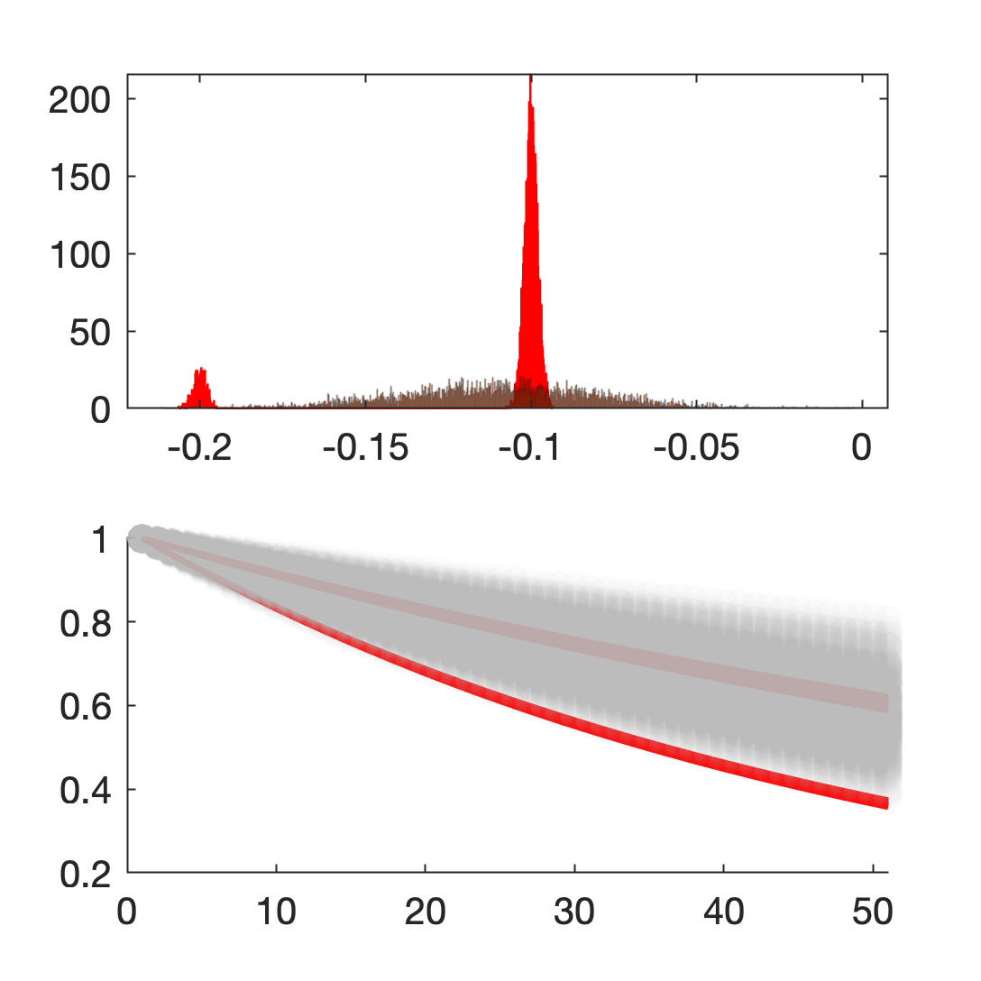
Figure 2: (top). Histogram approximating the uncertain parameter density for IVP example. (Red) the histogram represents the initial parameter $\xi\sim\mathrm{GMM}$, (Gray) the histogram represents $\ \xi^{\prime}\sim N(m,\sigma)$. The two distributions match up to the second moment. However, the GMM is skewed. (bottom). Two stochastic ODE states with parameter $\xi$ (red) and $\xi^{\prime}$ (gray). The states are obtained as a result of forward Euler integration.

We wish to answer: can we quantify the different behaviors of those systems without imposing distribution assumptions? To this end, we apply Algorithm 1 to obtain two sets of propagated system states $\{x(t,\xi^{i})\}_{i=1}^{N}$ and $\{x(t,{{\xi^{\prime}}^{i}})\}_{i=1}^{N}$. The state KME estimator $\hat{\mu}_{X_{t}}$ and $\hat{\mu}_{X_{t}^{\prime}}$ are computed using (6).

As illustrated in Figure 2 (bottom), the two moment-matched parameter distributions result in distinct system behaviors over time. To quantitatively compare the behaviors, we compute the RKHS-distance over time between those two embeddings $\|\hat{\mu}_{X_{t}}-\hat{\mu}_{X_{t}^{\prime}}\|_{\mathcal{H}}$ using (7).

To understand how different kernels preserve statistical properties of the system, we also plotted the embedding distances associated with polynomial kernel of order $1-4$ in Figure 3 (bottom). We clearly observe that different polynomial kernels capture different orders of moment information. Notably, the two system states seem to have similar means and therefore the first order polynomial kernel does not differentiate the two systems. As we increase the order of the polynomial kernel, the difference becomes evident.

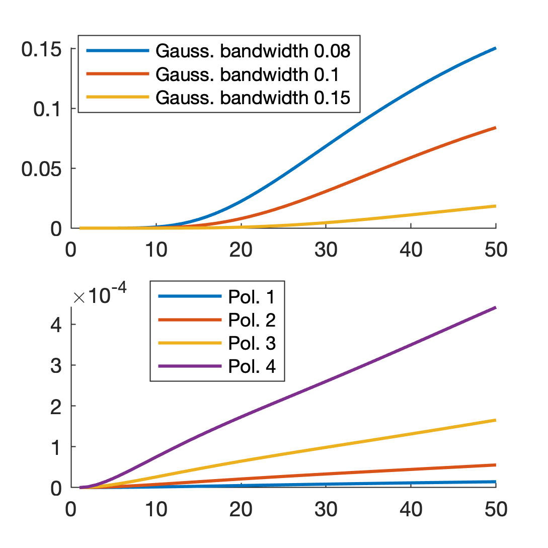
Figure 3: (top): RKHS distance over time between two embeddings $\|\hat{\mu}_{X_{t}}-\hat{\mu}_{X_{t}^{\prime}}\|_{\mathcal{H}}$ associated with Gaussian kernel of different bandwidth. (bottom): Embedding distances associated with polynomial kernel of order $1-4$.

We then show the Gaussian kernel embeddings in Figure 3 (top), where we vary the bandwidth parameter $\sigma$. It can be shown that the Gaussian kernel keeps track of statistical moments up to infinite order. If bandwidth is large, the kernel treats everything the same so RKHS distance is small. On the other hand, if bandwidth is small, the kernel treats everything as different. In the limiting case as the bandwidth $\to 0$, it can be shown the KME estimation reduces to the usual Monte Carlo estimation [cf. Section 3.3 in Schölkopf et al. (2015)].

4.2 Distribution-free goodness-of-fit for identification

To demonstrate the proposed technique is a good measure of goodness-of-fit for arbitrary uncertainty distributions, we apply it to PVE example in Mohammadi et al. (2015). Different from the uncertainty description in Section 4.1, this is typically a “worst-case” scenario where the model needs to account for the worst case realization of disturbances, described by ellipsoidal uncertainty sets.

In this example, the model to be identified is a time-varying autoregressive exogenous-input model (ARX) with variable parameter.

$$y_{k}=a^{1}y_{k-1}+a^{2}y_{k-2}+b^{1}u_{k-1}.$$

The uncertain time-varying parameters are $w=(a^{2},b^{1})$. To generate the data, we follow the setup of Mohammadi et al. (2015) to choose the true uncertain parameters $w^{i}$ uniformly randomly within the true ellipsoidal uncertainty set $\mathcal{E}(\bar{w},Z)$. The identification was performed according to that paper. As a result, we obtain the estimated ellipsoid $\mathcal{E}(w_{\text{PVE}},Z_{\text{PVE}})$ and the LSQ parameter $w_{\text{LSQ}}$ , as illustrated in Figure 4 (left).

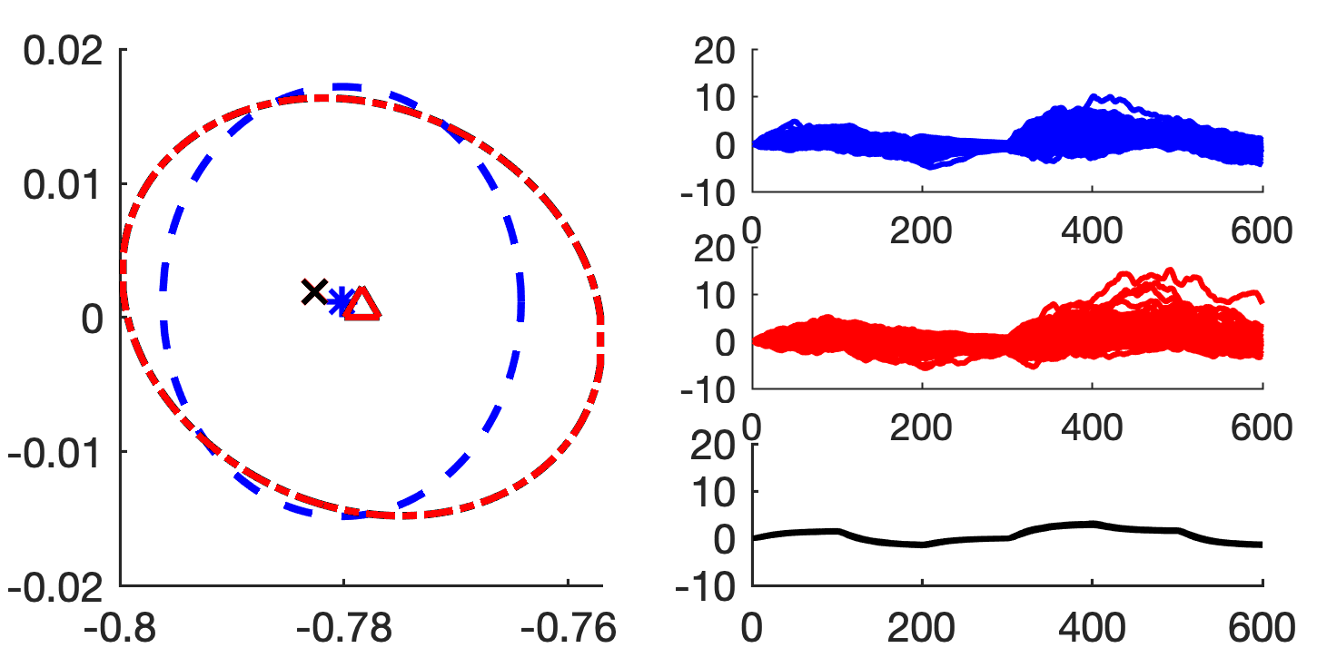
Figure 4: (left) plots the true uncertainty set (blue), estimated ellipsoidal uncertainty set (red), as well as the LSQ point estimate (black). (right) plots the result of evolving the system for 600 steps using true ellipsoid (blue), estimated variability ellipsoid using PVE (red), Gaussian distributed parameter variability from LSQ (black).

We evolve the system for 600 steps using the true model and those two different uncertain parameter models (PVE vs. Gaussian distributed parameter $w\sim\mathcal{N}(w_{\mathrm{LSQ}},Z_{\mathrm{LSQ}})$ resulting from the LSQ assumption, where $Z_{\mathrm{LSQ}}$ is estimated by the sample variance as in that paper). The resulting state trajectories are shown in Figure 4 (right). We apply Algorithm 1 and compute the RKHS distance $\|\hat{\mu}_{X(t,\hat{\xi}_{\mathrm{PVE/LSQ}})}-\hat{\mu}_{X(t,\xi^{*})}\|_{\mathcal{H}}$ between the embeddings of the estimated model and the true model. Figure 5 demonstrates that the PVE model (red) matches the true model better than the LSQ model (black) in the sense of RKHS metric. This comparison is performed under no distributional assumptions.

In that paper, it is obvious that LSQ did not deliver the parameter variability that fits the true generating distribution. However, one may ask, is the LSQ estimated parameter $\xi_{\mathrm{LSQ}}$ nonetheless able to deliver similar system behaviors? But there was no unified way to compare them. This paper provides a unifying framework to quantitatively answer this question.

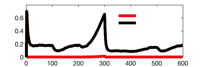
Figure 5: We show goodness-of-fit using $\|\hat{\mu}_{X(t,\hat{\xi}_{\mathrm{PVE}})}-\hat{\mu}_{X(t,\xi^{*})}\|_{\mathcal{H}}$ for estimated parameter variability using PVE (red), and $\|\hat{\mu}_{X(t,\hat{\xi}_{\mathrm{LSQ}})}-\hat{\mu}_{X(t,\xi^{*})}\|_{\mathcal{H}}$ for Gaussian-distributed parameter from LSQ estimation (black). They correspond to the system evolution over time in Figure 4 (right).

4.3 Recursive reduced set KPP for uncertainty propagation

Relying on the statistical consistency results in Section 2, uncertainty propagation can be performed straightforwardly using Algorithm 1. In this section, we demonstrate the use of Algorithm 2. As a proof of concept, let us consider a simple discrete-time stochastic system

$$x(t+1)=x(t)+w(t),w(t)\sim\mathrm{Uniform}\left(-\frac{1}{2},\,\,\,\frac{1}{2}\right)+0.1t.$$

We emphasize the distribution of $w(t)$ could be made fairly arbitrary (and non-stationary)— the proposed propagation method does not place restrictions on this distribution. The system evolution is illustrated in Figure 6 (left).

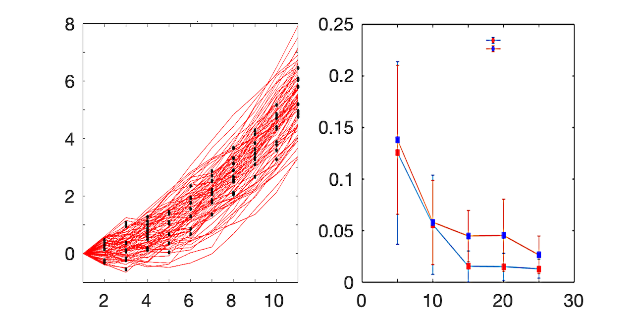
Figure 6: (left) Uncertainty propagation using reduced set method. The uncertainty is forward propagated for 10 steps, using the reduced set methods of size parameter 10. The red lines are Monte Carlo simulations of the system in question. The black dots are chosen reduced set to represent the state distribution at each time step. (right) Comparing approximation errors of the recursive reduced set algorithm (red, Alg. 2), $\|\hat{\mu}_{\tilde{x}_{t}}-\mu_{x_{t}}\|^{2}_{\mathcal{H}}$, with that of the diagonal estimate of KME (blue, Alg. 1)). The dynamics are run for 10 steps. Each method is run 10 times to produce the error bar plot. The state is sampled at time step $t=10$. In calculating the embedding , we use a Gaussian kernel with bandwidth $0.5$.

At every time step, Algorithm 2 is applied to find an embedding of the current state $\mu_{\tilde{x}_{t}}=\sum_{i\in\mathcal{R}}\alpha_{i}k(x_{t}^{i},\cdot)$, where $\mathcal{R}$ denotes the reduced-set indices. Then the dynamics is propagated forward again. Note we use the naive reduced set method following Simon-Gabriel et al. (2016) which simply samples expansion points $\{x_{t}^{i}\}$ from the full set and then solves a quadratic minimization problem for coefficients $\{\alpha^{i}\}$ as in Step 5. A more sophisticated method will be introduced in future work. As illustrated in Figure 6 (left), This procedure is repeated for 10 time steps. We compare the RKHS approximation error $\|\hat{\mu}_{\tilde{x}_{t}}-\mu_{x_{t}}\|^{2}_{\mathcal{H}}$ of the recursive reduced set method in Algorithm 2, against that of the diagonal estimate of Algorithm 1. While we do not know the true embedding $\mu_{x_{t}}$, we approximate it with a large-sample estimate using 500 samples. The approximation error in RKHS metric are illustrated in Figure 6 (right). We observe a faster convergence in both mean and variance by the recursive reduced set method in Algorithm 2.

5 Discussion

This paper proposed to use kernel probabilistic programming as a unifying tool for treating uncertainties in dynamical systems. We demonstrated concrete numerical procedures of propagating the uncertainty in dynamics. It is our on-going endeavor to investigate more sophisticated optimization procedures as well as mathematically rigorous analysis of convergence in Algorithm 2 with more general numerical integration. Another important direction is distributionally robust control design and state estimation using RKHS embeddings.

Compared with existing popular methods such as gPC or GP, RKHS embedding methods for dynamical systems are still in the early development. This paper serves as a call to action for their wider applications to robust and stochastic control.

We would like to thank Mario Zanon for providing the code to reproduce the PVE experiment.

Appendix A Proof of Lemma 9

We provide a proof for the consistency of Algorithm 1.

$$\begin{array}[]{ll}\|\hat{\mu}_{\hat{F}(x,\xi,t)}-\mu_{F(x,\xi,t)}\|=\|\hat{\mu}_{\hat{F}(x,\xi,t)}-\hat{\mu}_{F(x,\xi,t)}\\ +\hat{\mu}_{F(x,\xi,t)}-\mu_{F(x,\xi,t)}\|\\ \leq\|\hat{\mu}_{\hat{F}(x,\xi,t)}-\hat{\mu}_{F(x,\xi,t)}\|+\|\hat{\mu}_{F(x,\xi,t)}-\mu_{F(x,\xi,t)}\|\\ \leq C\cdot\|{\hat{F}(x,\xi,t)}-{F(x,\xi,t)}\|+\|\hat{\mu}_{F(x,\xi,t)}-\mu_{F(x,\xi,t)}\|\\ \to 0\end{array}$$ (15)

In the last inequality, The first term is due to the continuity of kernel $k$. In the last line, the first term converges to $0$ due to the consistency of numerical integration whereas the second term converges due to the consistency of KPP in Proposition 9.

The convergence rate is $\mathcal{O}(h^{p})+\mathcal{O}(\frac{1}{\sqrt{N}})$. The first term is the result of p-th order one-step numerical integration rule (e.g. RK-p) with step size $h$. The second term is triggered by The KPP estimator finite-sample convergence. $N$ is the sample size used by the KPP algorithm.

References

- Boots et al. (2013) Boots, B., Gordon, G., and Gretton, A. (2013). Hilbert space embeddings of predictive state representations. arXiv preprint arXiv:1309.6819.
- Campi et al. (2019) Campi, M.C., Garatti, S., and Prandini, M. (2019). Scenario optimization for mpc. In Handbook of Model Predictive Control, 445–463. Springer.
- Fukumizu et al. (2004) Fukumizu, K., Bach, F., and Jordan, M. (2004). Dimensionality reduction for supervised learning with reproducing kernel Hilbert spaces. Journal of Machine Learning Research, 5, 73–99.
- Gauss (1815) Gauss, C.F. (1815). Methodus nova integralium valores per approximationem inveniendi. apvd Henricvm Dieterich.
- Gretton et al. (2012) Gretton, A., Borgwardt, K., Rasch, M., Schölkopf, B., and Smola, A. (2012). A kernel two-sample test. Journal of Machine Learning Research, 13, 723–773.
- Grünewälder et al. (2012) Grünewälder, S., Lever, G., Baldassarre, L., Pontil, M., and Gretton, A. (2012). Modelling transition dynamics in MDPs with RKHS embeddings. In Proceedings of the 29th International Conference on Machine Learning, 535–542. Omnipress.
- Mohammadi et al. (2015) Mohammadi, A., Diehl, M., and Zanon, M. (2015). Estimation of uncertain ARX models with ellipsoidal parameter variability. 2015 European Control Conference, ECC 2015, (1), 1766–1771. 10.1109/ECC.2015.7330793.
- Muandet et al. (2017) Muandet, K., Fukumizu, K., Sriperumbudur, B., and Schölkopf, B. (2017). Kernel mean embedding of distributions: A review and beyond. Foundations and Trends in Machine Learning, 10(1-2), 1–141.
- Nishiyama et al. (2012) Nishiyama, Y., Boularias, A., Gretton, A., and Fukumizu, K. (2012). Hilbert space embeddings of POMDPs. In Proceedings of the 28th Conference on Uncertainty in Artificial Intelligence, 644–653.
- Rasmussen and Williams (2006) Rasmussen, C.E. and Williams, C.K. (2006). Gaussian processes for machine learning. Gaussian Processes for Machine Learning, by CE Rasmussen and CKI Williams. ISBN-13 978-0-262-18253-9.
- Schölkopf et al. (2015) Schölkopf, B., Muandet, K., Fukumizu, K., Harmeling, S., and Peters, J. (2015). Computing functions of random variables via reproducing kernel Hilbert space representations. Statistics and Computing, 25(4), 755–766. 10.1007/s11222-015-9558-5.
- Schölkopf et al. (2002) Schölkopf, B., Smola, A.J., Bach, F., et al. (2002). Learning with kernels: support vector machines, regularization, optimization, and beyond. MIT press.
- Scokaert and Mayne (1998) Scokaert, P.O. and Mayne, D.Q. (1998). Min-max feedback model predictive control for constrained linear systems. IEEE Transactions on Automatic control, 43(8), 1136–1142.
- Simon-Gabriel et al. (2016) Simon-Gabriel, C.J., Ścibior, A., Tolstikhin, I., and Schölkopf, B. (2016). Consistent kernel mean estimation for functions of random variables. Advances in Neural Information Processing Systems, 1(i), 1740–1748.
- Smola et al. (2007) Smola, A.J., Gretton, A., Song, L., and Schölkopf, B. (2007). A Hilbert space embedding for distributions. In Proceedings of the 18th International Conference on Algorithmic Learning Theory (ALT), 13–31. Springer-Verlag.
- Song (2008) Song, L. (2008). Learning via Hilbert Space Embedding of Distributions. Ph.D. thesis, The University of Sydney.
- Song et al. (2013) Song, L., Fukumizu, K., and Gretton, A. (2013). Kernel embeddings of conditional distributions: A unified kernel framework for nonparametric inference in graphical models. IEEE Signal Processing Magazine, 30(4), 98–111.
- Sriperumbudur et al. (2010) Sriperumbudur, B., Gretton, A., Fukumizu, K., Schölkopf, B., and Lanckriet, G. (2010). Hilbert space embeddings and metrics on probability measures. Journal of Machine Learning Research, 99, 1517–1561.
- Tempo et al. (2012) Tempo, R., Calafiore, G., and Dabbene, F. (2012). Randomized algorithms for analysis and control of uncertain systems: with applications. Springer Science & Business Media.
- Xiu (2009) Xiu, D. (2009). Fast numerical methods for stochastic computations: a review. Communications in computational physics, 5(2-4), 242–272.
- Xiu and Karniadakis (2002) Xiu, D. and Karniadakis, G.E. (2002). The wiener–askey polynomial chaos for stochastic differential equations. SIAM journal on scientific computing, 24(2), 619–644.