First hitting times to intermittent targets

Abstract

In noisy environments such as the cell, many processes involve target sites that are often hidden or inactive, and thus not always available for reaction with diffusing entities. To understand reaction kinetics in these situations, we study the first hitting time statistics of a Brownian particle searching for a target site that switches stochastically between visible and hidden phases. At high crypticity, an unexpected rate limited power-law regime emerges for the first hitting time density, which markedly differs from the classic $t^{-3/2}$ scaling for steady targets. Our problem admits an asymptotic mapping onto a mixed, or Robin, boundary condition. Similar results are obtained with non-Markov targets and particles diffusing anomalously.

Numerous phenomena are controlled by the time taken by a process to first reach a specified target state or conformation Redner (2001); Siegert (1951); Gardiner (2004). First passage processes allow us to understand diffusion controlled reactions Szabo et al. (1980); Cui et al. (2006), to predict the sizes of neuronal avalanches in neurocortical circuits Beggs and Plenz (2003) or the search strategies adopted by foraging animals Viswanathan et al. (2011); Kagan and Ben-Gal (2015). They are also supposed to govern the kinetics of many essential biological processes like antibody production or cell differentiation, which depend on how long it takes for fundamental steps to be completed, such as the first random encounter of two remote DNA segments Zhang and Dudko (2016); Chou and D’Orsogna (2014).

The theory of first passage processes has witnessed many recent developments Metzler et al. (2014), which usually consider fixed and perfectly absorbing targets. Naturally, in many cases, due to errors or imperfections in the binding or detection phase, reaction may occur only after several attempts. For instance, partial absorption is conveniently modeled through an absorption probability each time a random walker crosses a target region Majumdar and Bray (1998); Burkhardt (2000); Bray et al. (2013). In the Brownian limit this rule becomes equivalent to a radiation, or Robin, boundary condition, where the diffusive absorption flux is set proportional to the probability density at the target Redner (2001); Singer et al. (2008); Pal et al. (2018). Nevertheless, little is known on first passage problems with barriers or targets that follow some internal dynamicsBenichou et al. (1999); Bénichou et al. (2000); Rojo et al. (2011). A simple example, of interest here, is provided by switching processes between active and inactive states.

Stochastic switching processes are inherent in cell biology. Gene expression is only possible if a binding target site along the DNA chain is accessible to diffusive transcription factors McAdams and Arkin (1997); Tian and Burrage (2006). Instead of being continuous and smooth, transcription usually occurs in bursts separated by periods of inactivity during which no transcription is carried out Chubb and Liverpool (2010); Suter et al. (2011). Such transcriptional bursting is related to the chromatin remodeling state: when the chromatin is unfolded, the binding site is accessible for gene expression, whereas folded states do not allow transcription Munsky et al. (2012); Wu (1997); Eberharter and Becker (2002). The accessibility to the binding sites can be described by a Poisson distributed switching process, with fixed transitions rates between two states Munsky et al. (2012). In prokaryote cells such as E. coli, the time intervals between bursty (“on”) and silent (“off”) phases are exponentially distributed. These processes can have an average duration of minutes, the periods of inactivity being much longer than active periods Golding et al. (2005).

Switching between bistable states also characterizes DNA looping Wong et al. (2008) (the ability of distant sites on the chain to physically interact to regulate gene expression), where the time spent in the off-state can be also very long Chen et al. (2014). Similarly, ion channels stochastically transit between open and closed conformations, thus affecting transport through membranes, cell signaling or drug delivery Bressloff (2014); Reingruber and Holcman (2009). Studies on single ion-channels have shown that opening or closing events of the pore occur over characteristic dwell times ranging from 0.5 to hundreds of ms Kawano et al. (2013); Sakmann (2013). These times are comparable or much larger than the diffusion times of K⁺ or Ca²⁺ ions at the scale of a cell ($\tau_{D}\sim 0.1\ \mu$s) Donahue and Abercrombie (1988). Hence, first hitting times are likely to be limited by the channel state Lide (2004); Mashl et al. (2001).

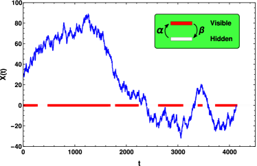
Figure 1: Brownian trajectory in the presence of an intermittent target located at the origin. The red segments represent the target in the visible state, separated by time intervals in the hidden state. The Brownian particle is absorbed when it reaches the target in the visible state for the first time.

In this Letter, we address the generic but largely unexplored question of a one-dimensional unbounded Brownian motion with diffusion coefficient $D$ and an intermittent target located at the origin, as illustrated in Figure 1. The target internal state is characterized by a time dependent binary variable $\sigma(t)$: when $\sigma=1$ the target is visible, meaning that the Brownian particle is absorbed upon encounter; when $\sigma=0$ the target is invisible or transparent, and the particle is not absorbed when crossing the origin. The target visibility randomly switches between these two states, which last for time intervals that are exponentially distributed. The target in state $\sigma=0$ changes to state $\sigma=1$ at rate $\alpha$, whereas the reverse transition occurs at rate $\beta$ (Fig. 1). Therefore, the mean duration of the visible (invisible) phase is $1/\beta$ ($1/\alpha$) and the probability to find the target in the visible state is $\alpha/(\alpha+\beta)$.

With one target, this problem bears similarities with an intermittent search (IS) strategy Bénichou et al. (2005, 2011), where the searcher becomes temporarily “blind”, the target being always visible. But unlike in IS, our particle does not adopt a different transport mode in the blind phase, it just keeps diffusing. For many targets with independent internal dynamics, the two problems differ even more.

A quantity of central interest here is $Q_{\sigma_{0}}(x,t)$, the probability that the particle has survived up to time $t$ given that its initial position was $x$, the initial target state being $\sigma(t=0)=\sigma_{0}$. We set $x>0$ in the following. Averaging over the initial target states defines the average survival probability, denoted as $Q_{\rm av}(x,t)$:

$$Q_{\rm av}(x,t)=\frac{\beta}{\alpha+\beta}Q_{0}(x,t)+\frac{\alpha}{\alpha+\beta}Q_{1}(x,t).$$ (1)

The first hitting time distribution (FHTD) $P_{i}$ is obtained from the usual identity $Q_{i}(x,t)=\int_{t}^{\infty}d\tau P_{i}(x,\tau)$ or

$$P_{i}(x,t)=-\frac{\partial Q_{i}(x,t)}{\partial t},$$ (2)

where $i\in\{0,1,{\rm av}\}$. Following a method applied to nonintermittent targets and Markov processes such as intermittent search Bénichou et al. (2011), run-an-tumble motion Malakar et al. (2018) or diffusion with resetting Evans and Majumdar (2018), we show in the Supplemental Material (SM) that the survival probabilities satisfy two coupled backward Fokker-Planck equations:

$$\frac{\partial Q_{0}(x,t)}{\partial t}= D\frac{\partial^{2}Q_{0}(x,t)}{\partial x^{2}}+\alpha\left[Q_{1}(x,t)-Q_{0}(x,t)\right]$$ (3)

$$\frac{\partial Q_{1}(x,t)}{\partial t}= D\frac{\partial^{2}Q_{1}(x,t)}{\partial x^{2}}+\beta\left[Q_{0}(x,t)-Q_{1}(x,t)\right].$$ (4)

These functions need to satisfy the boundary conditions

$$Q_{1}(x=0,t) = 0$$ (5)

$$\frac{\partial Q_{0}(x,t)}{\partial x}\Big{|}_{x=0} = 0.$$ (6)

Whereas Eq. (5) simply asserts that the target is absorbing in the visible state, relation (33) is a bit more subtle. It can be understood, for instance, by considering the case $\beta=0$ and a target in state $0$ at $t=0$, which therefore irreversibly transits to the visible state at rate $\alpha$. The calculation of $Q_{0}$ in this case is performed in the SM by using simple probabilistic arguments. One checks a posteriori that the solution fulfills condition (33). Similar arguments allow us to show that Eq. (33) holds in the general case $\beta>0$ as well (see the SM).

Let us define the Laplace transforms $\widetilde{Q}_{\sigma_{0}}(x,s)=\int^{\infty}_{0}Q_{\sigma_{0}}(x,t)e^{-st}dt$, which satisfy the following system

$$D\frac{\partial^{2}\widetilde{Q}_{0}(x,s)}{\partial x^{2}}+\alpha\widetilde{Q}_{1}(x,s)-(\alpha+s)\widetilde{Q}_{0}(x,s)=-1$$ (7)

$$D\frac{\partial^{2}\widetilde{Q}_{1}(x,s)}{\partial x^{2}}+\beta\widetilde{Q}_{0}(x,s)-(\beta+s)\widetilde{Q}_{1}(x,s)=-1$$ (8)

The general solutions are $\widetilde{Q}_{0}(x,s)=Ae^{\pm a\sqrt{s}}-\alpha Be^{\pm a\sqrt{s+\alpha+\beta}}/\beta+1/s$ and $\widetilde{Q}_{1}(x,s)=Ae^{\pm a\sqrt{s}}+Be^{\pm a\sqrt{s+\alpha+\beta}}+1/s$, where we have employed the notation

$$a=x/\sqrt{D}.$$ (9)

Thus, $\tau_{D}\equiv a^{2}$ is the typical diffusion time to reach the target region. With the boundary conditions (5)-(33) and noting that $Q_{\sigma_{0}}$ must remain finite as $a\rightarrow\infty$, one deduces

$$\widetilde{Q}_{i}(x,s)= -\frac{\alpha\sqrt{s+\alpha+\beta}}{\sqrt{s}\left(\alpha\sqrt{s+\alpha+\beta}+\beta\sqrt{s}\right)}\Bigg{(}\frac{e^{-a\sqrt{s}}}{\sqrt{s}}$$ (10)

$$-C_{i}\frac{e^{-a\sqrt{s+\alpha+\beta}}}{\sqrt{s+\alpha+\beta}}\Bigg{)}+\frac{1}{s}$$

where, again, $i=\{0,1,{\rm av}\}$ and the constants $C_{i}$ take the values $C_{0}=1$, $C_{1}=-\frac{\beta}{\alpha}$ and $C_{av}=0$.

The Laplace transform of the FHTD is deduced from the general relation $\widetilde{P}_{i}(x,s)=1-s\widetilde{Q}_{i}(x,s)$, which stems from Eq. (2). The solutions for $\widetilde{Q}_{i}$ or $\widetilde{P}_{i}$ do not seem to have simple inverses, nevertheless Eq. (47) can be inverted by means of the convolution theorem and the complete solution expressed in a rather lengthy integral form. This exact solution is given in the SM.

With the Laplace expressions (47) at hand, one easily checks that in the limit $\beta\rightarrow 0$, one recovers the well-known case of a target always in the visible state:

$$\widetilde{Q}_{{\rm av}}(x,s)\rightarrow\widetilde{Q}^{{\rm st}}(x,s)=\frac{1-e^{-a\sqrt{s}}}{s},$$ (11)

or $\widetilde{P}^{\rm st}(x,s)=e^{-a\sqrt{s}}$, where the label “st” stands for the standard case of a nonintermittent target Redner (2001). This expression is inverted as the Lévy-Smirnov distribution

$$P^{st}(a,t)=\frac{a}{\sqrt{4\pi t^{3}}}e^{-\frac{a^{2}}{4t}}\simeq\frac{a}{\sqrt{4\pi}}\ t^{-\frac{3}{2}}\ \ {\rm for}\ t\gg\tau_{D}.$$ (12)

For very large values of the two transition rates compared to the inverse diffusion time $1/a^{2}$, and keeping $\beta/\alpha$ constant, Eq. (47) shows that the three FHTDs also tend to that of the standard problem:

$${Q}_{i}(x,t)\rightarrow{Q}^{st}(x,t).$$ (13)

This result may seem counterintuitive, as it tells that at very high transition rates, the target is easily detectable by the Brownian particle, even if it is invisible most of the time, i.e., with $\beta/\alpha$ fixed to a large value. The fast absorption can be understood here by the recurrence of Brownian trajectories in $1d$: a particle crossing the origin re-crosses it many times within a short period. If, in the meantime, the target rapidly transits from one state to the other, as soon as it becomes visible, it will be hit by the nearby particle. A similar mechanism can explain the fast absorption of ligands that spend most of the time in a hidden state Reingruber and Holcman (2009).

We next comment on a key property which is not met with steady targets or in usual radiation boundary problems. In the limit of infinitely fast diffusion, $D\rightarrow\infty$ or $a\rightarrow 0$, a steady target is found immediately [$Q^{st}(a=0,t)=0$], since Brownian motion is recurrent in $1d$. In contrast, $Q_{\rm av}$ and $Q_{0}$ admit non-trivial limits for intermittent targets. Defining $Q^{I}_{i}(t)\equiv Q_{i}(a=0,t)$, the survival probability for any $a$ can be decomposed as:

$$Q_{i}(a,t)=Q^{I}_{i}(t)+Q^{D}_{i}(a,t)$$ (14)

where $i=\{0,{\rm av}\}$. By construction, $Q^{D}_{i}(a,t)$ vanishes as $a\rightarrow 0$ and represents the diffusion limited part of the survival probability, whereas $Q^{I}_{i}(t)$, which depends only on $\alpha$ and $\beta$, is the contribution limited by the target dynamics. This intermittent part arises from the fact that the target can be initially invisible and therefore undetectable while it remains so, no matter how fast diffusion occurs. $Q^{I}_{0}(t)$ is the probability that the particle starting right at the position of the initially invisible target, has still not hit it at $t$. Owing to Eq. (2), $P_{i}(a,t)$ can also be decomposed as $P^{I}_{i}(t)+P^{D}_{i}(a,t)$. From Eq. (47), one obtains in the Laplace domain

$$\widetilde{Q}^{I}_{0}(s)=\frac{\beta+\alpha}{\sqrt{s}(\alpha\sqrt{s+\alpha+\beta}+\beta\sqrt{s})},$$ (15)

whereas $\widetilde{Q}_{\rm av}^{I}(s)=\frac{\beta}{\alpha+\beta}\widetilde{Q}^{I}_{0}(s)$.

We now show how this intermittent contribution drastically affects the asymptotic properties of the FHTD, especially in the cryptic regime $\beta/\alpha\gg 1$. Since $\widetilde{Q}_{av}(a,s=0)=\infty$, the mean first hitting time is infinite like in the standard case, and we can deduce the large time behaviors from a small $s$ expansion. Approximating $\sqrt{s+\alpha+\beta}$ by $\sqrt{\alpha+\beta}$, Eq. (47) is recast as

$$\widetilde{Q}_{\rm av}(a,s)\simeq\frac{1}{s}\left(1-\frac{e^{-a\sqrt{s}}}{1+K\sqrt{s}}\right)$$ (16)

with $K=\beta/(\alpha\sqrt{\alpha+\beta})$. The right-hand-side of Eq. (16) can be exactly inverted Abramowitz and Stegun (1965) and combined with Eq. (2), yielding:

$$P_{\rm av}(a,t)\simeq \frac{1}{K\sqrt{\pi t}}\exp\left(-\frac{a^{2}}{4t}\right)$$ (17)

$$-\frac{1}{K^{2}}\operatorname{erfc}\left(\frac{\sqrt{t}}{K}+\frac{a}{2\sqrt{t}}\right)\exp\left(\frac{a}{K}+\frac{t}{K^{2}}\right).$$

Eq. (17) is valid for times larger than the target time-scale defined as $\tau_{ta}\equiv(\alpha+\beta)^{-1}$. It is very close to the exact solution obtained by convolution in the SM for all $t$ (see Fig. 2). Two scaling regimes emerge, as can be seen directly from Eq. (16) by setting $a\sqrt{s}\ll 1$:

1. For $K\sqrt{s}\ll 1$, one has $\widetilde{Q}_{\rm av}\simeq(a+K)/\sqrt{s}$, which is inverted as $Q_{\rm av}(a,t)\simeq(a+K)/\sqrt{\pi t}$. Hence, with Eq. (2), the asymptotic scaling (12) generalizes to

   $$P_{\rm av}(a,t)\simeq(a+K)/\sqrt{4\pi t^{3}}.$$ (18)

   

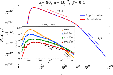
   Figure 2: Average first hitting time density in a cryptic case. The searcher starting position is $x=50$, and $D=1/2$. The crossover time $K^{2}$ is $\approx 10^{13}$ in this example. Inset: Average FHTD for $\alpha=10^{-4}$ and varying $\beta$. Symbols represent simulation results and lines the exact solution.

2. If $K\gg a$, an intermediate regime is possible, where $a\sqrt{s}\ll 1$ but $K\sqrt{s}\gg 1$ . In this case $\widetilde{Q}_{\rm av}\simeq\frac{1}{s}\left[1-1/(K\sqrt{s})\right]$, or $\widetilde{P}_{\rm av}=1-s\widetilde{Q}_{\rm av}\simeq 1/(K\sqrt{s})$. Hence,

   $$P_{\rm av}(a,t)\simeq 1/(K\sqrt{\pi t}).$$ (19)

Eq. (19) is one of our main results. From the above considerations, $\tau_{c}\equiv K^{2}$ sets a crossover time separating the standard $t^{-3/2}$ scaling (with a modified prefactor) from a new intermediate regime with exponent $-1/2$, holding in the range ${\rm max}(\tau_{ta},\tau_{D})\ll t\ll\tau_{c}$. This regime is intermittency dominated, as Eq. (19) does not involve $a$. Clearly, it can be observed only if $\tau_{c}/\tau_{ta}\gg 1$. As

$$\tau_{c}/\tau_{ta}=(\beta/\alpha)^{2},$$ (20)

the intermediate region exists for $\beta/\alpha\gg 1$, at high crypticity, and its extent rapidly increases with $\beta/\alpha$. As shown by Figure 2, this scaling law can span many decades, broadening considerably the FHTD and making the standard regime hard to reach. Meanwhile, $Q_{\rm av}(a,t)\simeq 1-(2/\sqrt{\pi})\sqrt{t/\tau_{c}}$ remains close to unity [see inset of Fig. 3-Left], i.e., target encounters are very rare.

At short times ($t\ll\tau_{ta}$), Eq. (17) is not valid and the FHTD can be deduced from a large $s$ expansion. Setting $a=0$ for simplicity, one gets from Eq. (15): $\widetilde{Q}^{I}_{\rm av}(s)\simeq\frac{\alpha}{(\alpha+\beta)s}\left[\frac{\beta}{\alpha}-\frac{\beta}{2s}+\frac{\beta(3\alpha+\beta)}{8s^{2}}+\cdots\right]$, which by inversion yields

$$P^{I}_{\rm av}(t)\simeq\frac{\alpha}{\alpha+\beta}\left[\delta(t)+\frac{\beta}{2}-\frac{\beta(3\alpha+\beta)}{8}t+\cdots\right].$$ (21)

The exact solution obtained in the SM is checked successfully with Monte Carlo simulations in Figure 2-Inset for several crypticity strengths. The intermediate regime is already noticeable at $\beta/\alpha\approx 10$. Note that biological systems are often cryptic and with $\tau_{c}\gg\tau_{D}$. Transcriptional bursting in prokaryotic cells is characterized by relatively short periods during which transcription is allowed, corresponding to $\beta/\alpha\approx 6$ Golding et al. (2005). Lactose repressors can also form long-tether DNA loops (that block transcription) at a rate $10$ times faster in than the loop$\rightarrow$unlooped transition Wong et al. (2008). The activity times $\tau_{c}$ in these examples are of the order of minutes, much larger than $\tau_{D}\sim 1$ s for a protein in a cell Goulian and Simon (2000). In presynaptic processes, the parametrized Hodgkin–Huxley model predicts a $\beta/\alpha$ of $\approx 4500$ for the switching rate to the inactivated state of Na⁺ channels at rest voltage ($50$ mV)Bressloff (2014); Ermentrout and Terman (2010).

Since the target switches between absorbing and hidden phases (the latter being equivalent to reflecting in the present geometry), one may wonder about a possible connection with diffusion in the presence of a mixed, or Robin, boundary condition (RBC). Let $p(z,t)$ be the probability density of the position $z\in[0,\infty)$ of a Brownian particle with a RBC at the origin, namely Singer et al. (2008):

$$\left.D\frac{\partial p}{\partial z}\right|_{z=0}=\kappa p(z=0,t),$$ (22)

where $\kappa$ is a positive constant. Eq. (22) is widely used in effective medium descriptions of spatially heterogeneous interfaces containing both reflecting and reactive zones Zwanzig (1990); Batsilas et al. (2003); Berezhkovskii et al. (2004). The exact survival probability in $1d$ of a particle starting at $z=x$ and obeying a RBC actually coincides with our Eq. (16) or (17) for all $t$, where $K$ must be replaced by $\sqrt{D}/\kappa$ Sano and Tachiya (1979); Pal et al. (2018). Consequently, as far as survival is concerned, both problems become equivalent at large times. We deduce the formula

$$\kappa=\frac{\alpha}{\beta}\sqrt{\alpha+\beta}\sqrt{D}.$$ (23)

As one may expect, the boundary is absorbing ($\kappa\rightarrow\infty$) when $\beta\rightarrow 0$ and reflecting ($\kappa\rightarrow 0$) when $\alpha\rightarrow 0$. Non trivially, it is also absorbing as $\alpha,\beta\rightarrow\infty$, $\beta/\alpha$ being fixed, as mentioned earlier. The two-state process thus provides a new, rigorous example of application of the RBC (22), extending the relevance of the latter to the study of fluctuating biophysical systems. Both problems differ for $t$ smaller than the target time-scale, though, as the RBC does not involve such a time-scale. A similar asymptotic analogy with the RBC was shown some time ago for diffusion into a partially absorbing medium Ben-Naim et al. (1993).

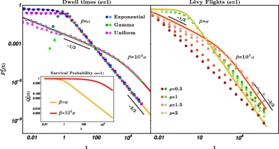
Figure 3: First hitting time density for a particle starting at the origin. Symbols represent simulation results and lines the exact solution obtained from Eq. (15). Left: Brownian particle and several distributions of activity/inactivity times: exponential, Gamma (with shape parameter $5$) and uniform. In each case, the mean time of the “off” (“on”) state is set to $1/\alpha$ ($1/\beta$, respectively). Right: Discrete Lévy flights of index $\mu$ and time-step $10^{-4}$, with an exponential target.

We discuss the generality of our findings when more complex processes come into play. On-off processes such as DNA looping or ion channel dynamics can be substantially non-Markov Colquhoun and Sakmann (1981); Liebovitch et al. (1987); Goychuk and Hänggi (2004). We have simulated targets with activity and inactivity times that were distributed non-exponentially in several ways. As shown by Figure 3-Left, the scaling regimes (18) and (19) still hold in those cases, and our previous solution remains quantitatively correct at large times [$t>$max$(1/\alpha,1/\beta$)].

The Brownian motion case can also be extended to anomalous transport. Given a Markovian target, we simulated searchers performing one step per time unit ($\Delta t\ll 1/\alpha$ and $1/\beta$), i.e., with position $X_{n}=\sum_{i=1}^{n}\ell_{i}$ with $t=n\Delta t$, and where the i.i.d. $\ell_{i}$’s follow a symmetric Lévy stable distribution of index $0<\mu<2$ Chambers et al. (1976). The process terminates when $X_{n}$ changes sign while the target is active. In the border case $\mu=2$, the distribution of the $\ell_{i}$’s was $\propto|\ell|^{-3}$. For $\beta\sim\alpha$, the FHTD for a particle starting at the origin (with $\sigma_{0}=0$) depends surprisingly little on $\mu$ and is close to the Brownian curve, see Fig. 3-Right. Although approximate, this independence is reminiscent of the universality of the Sparre Andersen theorem, valid for any unbiased continuous $1d$ process being absorbed when first crossing the origin Feller (2008). If $\beta\gg\alpha$, the process crosses the origin many times before absorption. The intermediate regime appears, as for Brownian motion. However, the corresponding exponent $\zeta_{\mu}$ continuously depends on $\mu$: $\zeta_{2}\approx-1/2$ whereas $\zeta_{1}\approx\zeta_{1/2}\approx-1$. Except for $\mu=2$, the $-3/2$ regime was not observed as it may settle at very large times.

In summary, we have shown that diffusive search processes can be severely affected by the intermittent switching dynamics of a target site, a situation often met in noisy complex media. A new, rate controlled scaling regime with exponent $-1/2$ emerges at high target crypticity, and the problem can be mapped onto a radiation boundary problem at large times. These results can be readily extended to higher spatial dimensions with the same formalism. Our findings point toward intermittent dynamics as a way of regulating first passage processes in the cell. They can also have implications in foraging ecology, where animals are able to be cryptic and undetectable by predators for long period of times by camouflaging themselves Stevens and Merilaita (2009), or adopting a subterranean lifestyle Edmunds (1990); Ruxton et al. (2004); Gendron and Staddon (1983); O’Brien et al. (1990). According to Eq. (23), to avoid predators and fulfill the constraint of spending a certain fraction of time outside, animals should space out consecutive exits in time, a behaviour actually observed in female ground squirrels Williams et al. (2014, 2016). Macroscopic search experiments with dynamical targets can be achieved by means of mobile robots with a limited sensing range and fixed sources emitting intermittent electromagnetic signals Song et al. (2011a, b). We finally mention that the decay of the survival probability in unconfined space plays an important role for the large volume scaling of the FHTD in confined environments Levernier et al. (2018). The intermediate regime for cryptic targets should thus have important consequences for confined walks Condamin et al. (2007).

We thank Germinal Cocho and PAPIIT-DGAPA through Grant IN108318 for support. G. M. V. thanks CONACYT for scholarship support. We thank O. Bénichou, P. Cluzel, A. Kundu, S. N. Majumdar, P. Miramontes, I. Pérez-Castillo, G. Schehr and F. J. Sevilla for fruitful discussions.

I Governing equations

We derive here the coupled backward Fokker-Planck equations satisfied by the survival probabilities $Q_{0,1}(x,t)$ and which read:

$$\frac{\partial Q_{0}(x,t)}{\partial t}=D\frac{\partial^{2}Q_{0}(x,t)}{\partial x^{2}}+\alpha[Q_{1}(x,t)-Q_{0}(x,t)]$$ (24)

$$\frac{\partial Q_{1}(x,t)}{\partial t}=D\frac{\partial^{2}Q_{1}(x,t)}{\partial x^{2}}+\beta[Q_{0}(x,t)-Q_{1}(x,t)]$$ (25)

We suppose that the Brownian particle starts from a position $x>0$ at time $t=0$, with the target in the initial state $\sigma_{0}=0$. We notice that during a small time interval $[0,\Delta t]$, the target can switch to the state $\sigma=1$ with probability $\alpha\Delta t$ or remain in $\sigma=0$ with probability $1-\alpha\Delta t$. Summing these two contributions, one obtains a relation for the quantity $Q_{0}(x,t+\Delta t)$:

$$Q_{0}(x,t+\Delta t)=\alpha\Delta t\int_{-\infty}^{\infty}d\xi P_{\Delta t}(\xi)Q_{1}(x+\xi,t)+(1-\alpha\Delta t)\int_{-\infty}^{\infty}d\xi P_{\Delta t}(\xi)Q_{0}(x+\xi,t)$$ (26)

At time $\Delta t$, the particle position is $x+\xi$, which serves as a new initial condition for the rest of the trajectory in the interval $[\Delta t,t+\Delta t]$, which is of duration $t$. The random displacement $\xi$ of the Brownian particle is drawn from the Gaussian distribution $P_{\Delta t}(\xi)$ with zero mean and variance $\langle\xi^{2}\rangle=2D\Delta t$. A Taylor expansion of the probabilities $Q_{0,1}(x+\xi,t)$ in powers of $\xi$ up to second order (the first non-zero average contribution) gives:

$$Q_{0,1}(x+\xi,t)=Q_{0,1}(x,t)+\xi\frac{\partial Q_{0,1}(x,t)}{\partial x}+\frac{\xi^{2}}{2}\frac{\partial^{2}Q_{0,1}(x,t)}{\partial x^{2}}+...$$ (27)

Similarly $Q_{0}(x,t+\Delta t)=Q_{0}(x,t)+\Delta t\frac{\partial Q_{0}(x,t)}{\partial t}+...$ After using the fact that $\langle\xi\rangle=0$ and $\langle\xi^{2}\rangle=2D\Delta t$, we group the terms of order $\Delta t$, take the limit $\Delta t\rightarrow 0$, and Eq. (24) is obtained. Eq. (25) is deduced from a similar reasoning, noting that now the probability to switch from the state $\sigma=1$ to $\sigma=0$ during the time interval $[0,\Delta t]$ is $\beta\Delta t$, whereas, with probability $1-\beta\Delta t$, the target will remain with $\sigma=1$.

II Boundary condition for $Q_{0}(x,t)$

We suppose that at $t=0$ the target site, which fixed at $x=0$, is in the dormant state $\sigma_{0}=0$. The probability that the target switches to the active state $\sigma=1$ for the first time at time $t^{\prime}$ is given by the exponential distribution with rate $\alpha$. If we choose $\beta=0$, once the target has switched to the active state, it will remain active for ever. Since the Brownian particle started at $x>0$ at $t=0$ and diffuses in the unbounded free space, it will be located at a Gaussianly distributed position $x^{\prime}$ at time $t^{\prime}$. This position $x^{\prime}$ represents a new initial position for the standard first passage problem with a permanent target. For $\beta=0$, the survival probability at time $t$ will thus be given by

$$Q_{0}(x,t)=\int_{0}^{\infty}dt^{\prime}\alpha e^{-\alpha t^{\prime}}\int_{-\infty}^{\infty}dx^{\prime}\frac{e^{-\frac{(x^{\prime}-x)^{2}}{4Dt^{\prime}}}}{\sqrt{4\pi Dt^{\prime}}}\times\begin{cases}1&\text{if $t^{\prime}>t$}\\ Q^{st}(x^{\prime},t-t^{\prime})&\text{if $t^{\prime}<t$}\end{cases}$$ (28)

where $Q^{st}(x,t)$ stands for the standard survival probability with a steady target. In Eq. (28), we have used the fact that the particle cannot be absorbed while the target is inactive ($t<t^{\prime}$), and the averages over $x^{\prime}$ and $t^{\prime}$ are taken. Let us also take the Laplace transform of Eq. (28), denoting $\widetilde{Q}_{0}(x,s)=\int_{0}^{\infty}dt\ e^{-st}Q_{0}(x,t)$. After changing the order of the integrals, we obtain

$$\widetilde{Q}_{0}(x,s)=\alpha\int_{0}^{\infty}dt^{\prime}e^{-\alpha t^{\prime}}\int_{-\infty}^{\infty}dx^{\prime}\frac{e^{-\frac{(x^{\prime}-x)^{2}}{4Dt^{\prime}}}}{\sqrt{4\pi Dt^{\prime}}}\left(\int_{0}^{t^{\prime}}dt\ e^{-st}+\int_{t^{\prime}}^{\infty}dt\ e^{-st}Q^{st}(x^{\prime},t-t^{\prime})\right)$$ (29)

The first integral of the second line of Eq. (29) is simply $\frac{1-e^{-st^{\prime}}}{s}$ and does not depend on $x^{\prime}$, thus, the integral over $x^{\prime}$ gives unity. For the second integral of the same line, we make a change of variable $u=t-t^{\prime}$ and obtain the Laplace transform of $Q^{st}(x,u)$ multiplied by a factor $e^{-st^{\prime}}$. Therefore:

$$\widetilde{Q}_{0}(x,s)= \alpha\int_{0}^{\infty}dt^{\prime}e^{-\alpha t^{\prime}}\Bigg{(}\frac{1-e^{-st^{\prime}}}{s}+e^{-st^{\prime}}\int_{-\infty}^{\infty}dx^{\prime}\frac{e^{-\frac{(x^{\prime}-x)^{2}}{4Dt^{\prime}}}}{\sqrt{4\pi Dt^{\prime}}}\widetilde{Q}^{st}(x^{\prime},s)\Bigg{)}$$ (30)

$$= \frac{1}{s+\alpha}+\alpha\int_{-\infty}^{\infty}dx^{\prime}\frac{e^{-|x^{\prime}-x|\sqrt{(s+\alpha)/D}}}{\sqrt{4D(s+\alpha)}}\widetilde{Q}^{st}(x^{\prime},s)$$

Given that $\widetilde{Q}^{st}(x^{\prime},s)=\frac{1-e^{-|x^{\prime}|\sqrt{s/D}}}{s}$ Redner (2001) we substitute this expression into Eq. (30) and obtain

$$\widetilde{Q}_{0}(x,s)=\frac{1}{s+\alpha}+\frac{\alpha}{2s{\sqrt{D(s+\alpha)}}}\int_{-\infty}^{\infty}dx^{\prime}e^{-|x^{\prime}-x|\sqrt{(s+\alpha)/D}}\left(1-e^{-|x^{\prime}|\sqrt{s/D}}\right)$$ (31)

After integrating in Eq. (31), we obtain

$$\widetilde{Q}_{0}(x,s)=\frac{1}{s}+\frac{\sqrt{s}e^{-x\sqrt{(s+\alpha)/D}}-\sqrt{s+\alpha}e^{-x\sqrt{s/D}}}{s\sqrt{s+\alpha}}.$$ (32)

This result coincides with Eq. (10) in the main text for the case $i=0$ and $\beta=0$. It is also easy to see that Eq. (32) satisfies the boundary condition

$$\frac{\partial\widetilde{Q}_{0}(x,s)}{\partial x}\Big{|}_{x=0}=0,$$ (33)

for any $s$, which implies that

$$\frac{\partial{Q}_{0}(x,t)}{\partial x}\Big{|}_{x=0}=0,$$ (34)

for any $t$. Hence, it is “as if” the boundary in $x=0$ was always reflective, given its initial reflecting state $\sigma=0$. This may look surprizing, since the target is actually reactive (absorbing) any time after the switch time $t^{\prime}$.

In the general case $\beta\neq 0$, the boundary condition can actually be derived in a similar way. As before, we suppose that the initial target state is $\sigma_{0}=0$. The particle starts from the position $x>0$ and freely diffuses until the first transition to the state $\sigma=1$ occurs, at a time $t^{\prime}$. During the interval $[0,t^{\prime}]$ the particle has reached the Gaussianly distributed position $x^{\prime}$. At this point, the deduction departs from the case of $\beta=0$; now, the survival probability function for times $t>t^{\prime}$ is no longer the standard survival probability but $Q_{1}(x^{\prime},t-t^{\prime})$, since a renewed diffusion process starts from $x^{\prime}$ with $\sigma_{0}=1$ at time $t^{\prime}$. Thus, the survival probability at time $t$ will be

$$Q_{0}(x,t)=\int_{0}^{\infty}dt^{\prime}\alpha e^{-\alpha t^{\prime}}\int_{-\infty}^{\infty}dx^{\prime}\frac{e^{-\frac{(x^{\prime}-x)^{2}}{4Dt^{\prime}}}}{\sqrt{4\pi Dt^{\prime}}}\times\begin{cases}1&\text{if $t^{\prime}>t$}\\ Q_{1}(x^{\prime},t-t^{\prime})&\text{if $t^{\prime}<t$}\end{cases}$$ (35)

In Eq. (35), $Q_{1}$ does not depend on the initial position $x$, thus the derivative with respect to $x$ will only apply to the exponential term in the integral. Evaluating $\partial Q_{0}(x,t)/\partial x$ in $x=0$ gives

$$\frac{\partial Q_{0}(x,t)}{\partial x}\Big{|}_{x=0}=\int_{0}^{\infty}dt^{\prime}\alpha e^{-\alpha t^{\prime}}\int_{-\infty}^{\infty}dx^{\prime}\frac{x^{\prime}e^{-\frac{x^{\prime 2}}{4Dt^{\prime}}}}{2Dt^{\prime}\sqrt{4\pi Dt^{\prime}}}\times\begin{cases}1&\text{if $t^{\prime}>t$}\\ Q_{1}(x^{\prime},t-t^{\prime})&\text{if $t^{\prime}<t$}\end{cases}$$ (36)

From the parity of the Gaussian function and of $Q_{1}$ with respect to $x^{\prime}$, namely, $Q_{1}(-x^{\prime},t-t^{\prime})=Q_{1}(x^{\prime},t-t^{\prime})$, we see that the integral over $x^{\prime}$ in Eq. (36) vanishes. Hence, we have shown that the boundary condition of Eq. (6) in the main text is valid for any $\beta$.

On the other hand, all the Monte Carlo simulations are in perfect agreement with the theoretical calculations, giving further support to the validity of the boundary conditions.

III Solution in the Laplace domain

In the Laplace domain, from Eqs. (24)-(25) we obtain the following system:

$$D\frac{\partial^{2}\widetilde{Q}_{0}(x,s)}{\partial x^{2}}+\alpha\widetilde{Q}_{1}(x,s)-(\alpha+s)\widetilde{Q}_{0}(x,s)=-1$$ (37)

$$D\frac{\partial^{2}\widetilde{Q}_{1}(x,s)}{\partial x^{2}}+\beta\widetilde{Q}_{0}(x,s)-(\beta+s)\widetilde{Q}_{1}(x,s)=-1$$ (38)

where the initial condition $Q_{\sigma}(x,t=0)=1$ has been used. The homogeneous part of Eqs. (37)-(38) admits solutions of the form $q_{0}e^{\lambda x}$ and $q_{1}e^{\lambda x}$ which satisfy

$$\begin{pmatrix}D\lambda^{2}-(\alpha+s)&\alpha\\ \beta&D\lambda^{2}-(\beta+s)\end{pmatrix}\begin{pmatrix}q_{0}\\ q_{1}\end{pmatrix}=0.$$ (39)

The eigenvalues are

$$\lambda_{1}=\pm\sqrt{\frac{s}{D}},\quad\lambda_{2}=\pm\sqrt{\frac{s+\alpha+\beta}{D}},$$ (40)

with their corresponding eigenstates:

$$v_{1}=\begin{pmatrix}1\\ 1\end{pmatrix},\quad v_{2}=\begin{pmatrix}-\frac{\alpha}{\beta}\\ 1\end{pmatrix}.$$ (41)

The inhomogeneous part of $\widetilde{Q}_{\sigma}$ is independent of $x$ and simply given by $1/s$ for $\sigma=0$ and $1$. Setting $x>0$, one notices that $\tilde{Q}_{\sigma}(x,s)$ must tend to $1/s$ as $x\rightarrow\infty$, since $Q_{\sigma}(x,t)$ remains equal to unity when the particle is very far from the target. Hence, only the negative eigenvalues are acceptable. One deduces

$$\tilde{Q}_{0}(x,s)=Ae^{-\sqrt{\frac{s}{D}}x}-\frac{\alpha}{\beta}Be^{-\sqrt{\frac{s+\alpha+\beta}{D}}x}+\frac{1}{s}$$ (42)

$$\tilde{Q}_{1}(x,s)=Ae^{-\sqrt{\frac{s}{D}}x}+Be^{-\sqrt{\frac{s+\alpha+\beta}{D}}x}+\frac{1}{s},$$ (43)

with $A$ and $B$ two constants. Let us use the notation

$$a=\frac{x}{\sqrt{D}}.$$ (44)

Enforcing the boundary condition $Q_{1}(x=0,t)=0$ as well as that given by Eq. (33) yields

$$A=-\frac{\alpha\sqrt{s+\alpha+\beta}}{s\left(\alpha\sqrt{s+\alpha+\beta}+\beta\sqrt{s}\right)}$$ (45)

$$B=-\frac{\beta}{\sqrt{s}\left(\alpha\sqrt{s+\alpha+\beta}+\beta\sqrt{s}\right)}.$$ (46)

The solutions are thus given by

$$\widetilde{Q}_{i}(a,s)=-\frac{\alpha\sqrt{s+\alpha+\beta}}{\sqrt{s}\left(\alpha\sqrt{s+\alpha+\beta}+\beta\sqrt{s}\right)}\Bigg{(}\frac{e^{-a\sqrt{s}}}{\sqrt{s}}-C_{i}\frac{e^{-a\sqrt{s+\alpha+\beta}}}{\sqrt{s+\alpha+\beta}}\Bigg{)}+\frac{1}{s}.$$ (47)

where $i=\{0,1,av\}$ and the constants $C_{i}$ take the values $C_{0}=1$, $C_{1}=-\frac{\beta}{\alpha}$ and $C_{av}=0$. Hence, the average survival probability, of particular interest in this study, reads

$$\widetilde{Q}_{av}(a,s)=\frac{1}{s}\left(1-\frac{\alpha\sqrt{s+\alpha+\beta}}{\alpha\sqrt{s+\alpha+\beta}+\beta\sqrt{s}}e^{-a\sqrt{s}}\right),$$ (48)

whereas $\widetilde{P}_{av}=1-s\widetilde{Q}_{av}$ is given by

$$\widetilde{P}_{av}(a,s)=\frac{\alpha\sqrt{s+\alpha+\beta}}{\alpha\sqrt{s+\alpha+\beta}+\beta\sqrt{s}}e^{-a\sqrt{s}},$$ (49)

IV Exact expressions for the $Q_{i}(x,t)$’s as convolutions

The general expressions (47)-(49) do not seem to admit exact inverse Laplace transforms in terms of elementary functions. We can nevertheless obtain $Q_{i}(a,t)$ by using the convolution theorem Spiegel (1965). To this end, we write Eq. (47) in terms of a product of two functions [Eqs. (50-51) below] and then determine its inverse through a convolution. We define:

$$f(s)=\frac{\sqrt{s}-\frac{\beta}{\alpha}\sqrt{s+\alpha+\beta}+\frac{\alpha+\beta}{\sqrt{s}}}{(\alpha-\beta)s+\alpha^{2}}$$ (50)

$$g_{i}(a,s)=\frac{e^{-a\sqrt{s}}}{\sqrt{s}}-C_{i}\frac{e^{-a\sqrt{s+\alpha+\beta}}}{\sqrt{s+\alpha+\beta}},$$ (51)

which are such that $Q_{i}(a,s)=1/s-\frac{\alpha^{2}}{\alpha+\beta}f(s)g_{i}(a,s)$. Denoting the inverse Laplace transforms of $f(s)$ and $g_{i}(a,s)$ as $F(t)$ and $G_{i}(a,t)$, respectively, we have:

$$Q_{i}(a,t)=1-\frac{\alpha^{2}}{\alpha+\beta}\int_{0}^{t}F(u)G_{i}(a,t-u)du.$$ (52)

The first hitting time distribution $P_{i}(a,t)$, is deduced from the general identity $P_{i}=-\partial Q_{i}/\partial t$, or:

$$P_{i}(a,t)=\frac{\alpha^{2}}{\alpha+\beta}\int_{0}^{t}F(u)\frac{\partial G_{i}(a,t-u)}{\partial t}du$$ (53)

where we have use the fact that $F(t)G_{i}(a,0^{+})=0$. The function $G_{i}(a,t)$ can be found by direct Laplace inversion Abramowitz and Stegun (1965):

$$G_{i}(a,t)=\frac{1}{\sqrt{\pi t}}e^{-\frac{a^{2}}{4t}}\left(1-C_{i}e^{-(\alpha+\beta)t}\right).$$ (54)

For $F(t)$, it is necessary to distinguish two cases: $\alpha=\beta$ and $\alpha\neq\beta$. By direct Laplace inversion we have Abramowitz and Stegun (1965)

where $\operatorname{erfi}(x)=-i\operatorname{erf}(ix)$ is the imaginary error function. In the main text, the exact first hitting time distribution (FHTD) are evaluated numerically using Eq. (53), (54) and (55).

References

- Redner (2001) S. Redner, A guide to first-passage processes (Cambridge University Press, Cambridge, England, 2001).
- Siegert (1951) A. J. Siegert, On the first passage time probability problem, Physical Review 81, 617 (1951).
- Gardiner (2004) C. Gardiner, Handbook of Stochastic Methods for Physics, Chemistry, and the Natural Sciences, Springer complexity (Springer, Berlin, 2004).
- Szabo et al. (1980) A. Szabo, K. Schulten, and Z. Schulten, First passage time approach to diffusion controlled reactions, The Journal of chemical physics 72, 4350 (1980).
- Cui et al. (2006) T. Cui, J. Ding, and J. Z. Chen, Mean first-passage times of looping of polymers with intrachain reactive monomers: Lattice Monte Carlo simulations, Macromolecules 39, 5540 (2006).
- Beggs and Plenz (2003) J. M. Beggsand D. Plenz, Neuronal avalanches in neocortical circuits, Journal of Neuroscience 23, 11167 (2003).
- Viswanathan et al. (2011) G. M. Viswanathan, M. G. Da Luz, E. P. Raposo, and H. E. Stanley, The physics of foraging: an introduction to random searches and biological encounters (Cambridge University Press, Cambridge, England, 2011).
- Kagan and Ben-Gal (2015) E. Kaganand I. Ben-Gal, Search and foraging: individual motion and swarm dynamics (Chapman and Hall/CRC, Boca Raton, FL, 2015).
- Zhang and Dudko (2016) Y. Zhangand O. K. Dudko, First-passage processes in the genome, Annual Review of Biophysics 45, 117 (2016).
- Chou and D’Orsogna (2014) T. Chouand M. R. D’Orsogna, First passage problems in biology, in First-Passage Phenomena and Their Applications (World Scientific, Singapore, 2014) pp. 306–345.
- Metzler et al. (2014) R. Metzler, G. Oshanin, and S. Redner (Eds.), First-passage phenomena and their applications (World Scientific, Singapore, 2014).
- Majumdar and Bray (1998) S. N. Majumdarand A. J. Bray, Persistence with partial survival, Physical Review Letters 81, 2626 (1998).
- Burkhardt (2000) T. W. Burkhardt, Dynamics of absorption of a randomly accelerated particle, Journal of Physics A: Mathematical and General 33, L429 (2000).
- Bray et al. (2013) A. J. Bray, S. N. Majumdar, and G. Schehr, Persistence and first-passage properties in nonequilibrium systems, Advances in Physics 62, 225 (2013).
- Singer et al. (2008) A. Singer, Z. Schuss, A. Osipov, and D. Holcman, Partially reflected diffusion, SIAM Journal on Applied Mathematics 68, 844 (2008).
- Pal et al. (2018) A. Pal, I. Pérez-Castillo, and A. Kundu, Motion of a brownian molecule in the presence of reactive boundaries, Physical Review E 100, 042128 (2019).
- Benichou et al. (1999) O. Benichou, B. Gaveau, and M. Moreau, Resonant diffusion in a linear network of fluctuating obstacles, Physical Review E 59, 103 (1999).
- Bénichou et al. (2000) O. Bénichou, M. Moreau, and G. Oshanin, Kinetics of stochastically gated diffusion-limited reactions and geometry of random walk trajectories, Physical Review E 61, 3388 (2000).
- Rojo et al. (2011) F. Rojo, P. A. Pury, and C. E. Budde, Intermittent pathways towards a dynamical target, Physical Review E 83, 011116 (2011).
- McAdams and Arkin (1997) H. H. McAdamsand A. Arkin, Stochastic mechanisms in gene expression, Proceedings of the National Academy of Sciences 94, 814 (1997).
- Tian and Burrage (2006) T. Tianand K. Burrage, Stochastic models for regulatory networks of the genetic toggle switch, Proceedings of the National Academy of Sciences 103, 8372 (2006).
- Chubb and Liverpool (2010) J. R. Chubband T. B. Liverpool, Bursts and pulses: insights from single cell studies into transcriptional mechanisms, Current Opinion in Genetics & Development 20, 478 (2010).
- Suter et al. (2011) D. M. Suter, N. Molina, D. Gatfield, K. Schneider, U. Schibler, and F. Naef, Mammalian genes are transcribed with widely different bursting kinetics, Science 332, 472 (2011).
- Munsky et al. (2012) B. Munsky, G. Neuert, and A. Van Oudenaarden, Using gene expression noise to understand gene regulation, Science 336, 183 (2012).
- Wu (1997) C. Wu, Chromatin remodeling and the control of gene expression, Journal of Biological Chemistry 272, 28171 (1997).
- Eberharter and Becker (2002) A. Eberharterand P. B. Becker, Histone acetylation: a switch between repressive and permissive chromatin: Second in review series on chromatin dynamics, EMBO Reports 3, 224 (2002).
- Golding et al. (2005) I. Golding, J. Paulsson, S. M. Zawilski, and E. C. Cox, Real-time kinetics of gene activity in individual bacteria, Cell 123, 1025 (2005).
- Wong et al. (2008) O. K. Wong, M. Guthold, D. A. Erie, and J. Gelles, Interconvertible lac repressor—DNA loops revealed by single-molecule experiments, PLoS Biology 6, e232 (2008).
- Chen et al. (2014) Y.-J. Chen, S. Johnson, P. Mulligan, A. J. Spakowitz, and R. Phillips, Modulation of DNA loop lifetimes by the free energy of loop formation, Proceedings of the National Academy of Sciences 111, 17396 (2014).
- Bressloff (2014) P. C. Bressloff, Stochastic processes in cell biology, Vol. 41 (Springer, 2014).
- Reingruber and Holcman (2009) J. Reingruberand D. Holcman, Gated narrow escape time for molecular signaling, Physical Review Letters 103, 148102 (2009).
- Kawano et al. (2013) R. Kawano, Y. Tsuji, K. Sato, T. Osaki, K. Kamiya, M. Hirano, T. Ide, N. Miki, and S. Takeuchi, Automated parallel recordings of topologically identified single ion channels, Scientific Reports 3, 1995 (2013).
- Sakmann (2013) B. Sakmann, Single-channel recording (Springer Science & Business Media, 1983).
- Donahue and Abercrombie (1988) B. Donahueand R. Abercrombie, Free diffusion coefficient of ionic calcium in cytoplasm, Cell Calcium 8, 437 (1988).
- Lide (2004) D. R. Lide, CRC handbook of chemistry and physics, Vol. 85 (CRC Press, Boca Raton, FL, 2004).
- Mashl et al. (2001) R. J. Mashl, Y. Tang, J. Schnitzer, and E. Jakobsson, Hierarchical approach to predicting permeation in ion channels, Biophysical Journal 81, 2473 (2001).
- Bénichou et al. (2005) O. Bénichou, M. Coppey, M. Moreau, P. Suet, and R. Voituriez, Optimal search strategies for hidden targets, Physical Review Letters 94, 198101 (2005).
- Bénichou et al. (2011) O. Bénichou, C. Loverdo, M. Moreau, and R. Voituriez, Intermittent search strategies, Reviews of Modern Physics 83, 81 (2011).
- Malakar et al. (2018) K. Malakar, V. Jemseena, A. Kundu, K. V. Kumar, S. Sabhapandit, S. N. Majumdar, S. Redner, and A. Dhar, Steady state, relaxation and first-passage properties of a run-and-tumble particle in one-dimension, Journal of Statistical Mechanics: Theory and Experiment 2018, 043215 (2018).
- Evans and Majumdar (2018) M. R. Evansand S. N. Majumdar, Run and tumble particle under resetting: a renewal approach, Journal of Physics A: Mathematical and Theoretical 51, 475003 (2018).
- Abramowitz and Stegun (1965) M. Abramowitzand I. A. Stegun, Handbook of mathematical functions: with formulas, graphs, and mathematical tables, Vol. 55 (Courier Corporation, Dover, New York, 1965).
- Goulian and Simon (2000) M. Goulianand S. M. Simon, Tracking single proteins within cells, Biophysical Journal 79, 2188 (2000).
- Ermentrout and Terman (2010) G. B. Ermentroutand D. H. Terman, Mathematical foundations of neuroscience, Vol. 35 (Springer Science & Business Media, New York, 2010).
- Zwanzig (1990) R. Zwanzig, Diffusion-controlled ligand binding to spheres partially covered by receptors: an effective medium treatment., Proceedings of the National Academy of Sciences 87, 5856 (1990).
- Batsilas et al. (2003) L. Batsilas, A. M. Berezhkovskii, and S. Y. Shvartsman, Stochastic model of autocrine and paracrine signals in cell culture assays, Biophysical Journal 85, 3659 (2003).
- Berezhkovskii et al. (2004) A. M. Berezhkovskii, Y. A. Makhnovskii, M. I. Monine, V. Y. Zitserman, and S. Y. Shvartsman, Boundary homogenization for trapping by patchy surfaces, The Journal of Chemical Physics 121, 11390 (2004).
- Sano and Tachiya (1979) H. Sanoand M. Tachiya, Partially diffusion-controlled recombination, The Journal of Chemical Physics 71, 1276 (1979).
- Ben-Naim et al. (1993) E. Ben-Naim, S. Redner, and G. Weiss, Partial absorption and “virtual” traps, Journal of Statistical Physics 71, 75 (1993).
- Colquhoun and Sakmann (1981) D. Colquhounand B. Sakmann, Fluctuations in the microsecond time range of the current through single acetylcholine receptor ion channels, Nature 294, 464 (1981).
- Liebovitch et al. (1987) L. S. Liebovitch, J. Fischbarg, and J. P. Koniarek, Ion channel kinetics: a model based on fractal scaling rather than multistate markov processes, Mathematical Biosciences 84, 37 (1987).
- Goychuk and Hänggi (2004) I. Goychukand P. Hänggi, Fractional diffusion modeling of ion channel gating, Physical Review E 70, 051915 (2004).
- Chambers et al. (1976) J. M. Chambers, C. L. Mallows, and B. Stuck, A method for simulating stable random variables, Journal of the American Statistical Association 71, 340 (1976).
- Feller (2008) W. Feller, An introduction to probability theory and its applications, Vol. 2 (John Wiley & Sons, New York, 2008).
- Stevens and Merilaita (2009) M. Stevensand S. Merilaita, Animal camouflage: current issues and new perspectives, Philosophical Transactions of the Royal Society of London B: Biological Sciences 364, 423 (2009).
- Edmunds (1990) M. Edmunds, The evolution of cryptic coloration, Insect Defenses: Adaptive Mechanisms and Strategies of Prey and Predators , 3 (1990).
- Ruxton et al. (2004) G. D. Ruxton, T. N. Sherratt, M. P. Speed, M. P. Speed, M. Speed, et al., Avoiding attack: the evolutionary ecology of crypsis, warning signals and mimicry (Oxford University Press, Oxford, 2004).
- Gendron and Staddon (1983) R. P. Gendronand J. E. Staddon, Searching for cryptic prey: the effect of search rate, The American Naturalist 121, 172 (1983).
- O’Brien et al. (1990) W. J. O’Brien, H. I. Browman, and B. I. Evans, Search strategies of foraging animals, American Scientist 78, 152 (1990).
- Williams et al. (2014) C. T. Williams, K. Wilsterman, A. D. Kelley, A. R. Breton, H. Stark, M. M. Humphries, A. G. McAdam, B. M. Barnes, S. Boutin, and C. L. Buck, Light loggers reveal weather-driven changes in the daily activity patterns of arboreal and semifossorial rodents, Journal of Mammalogy 95, 1230 (2014).
- Williams et al. (2016) C. T. Williams, K. Wilsterman, V. Zhang, J. Moore, B. M. Barnes, and C. L. Buck, The secret life of ground squirrels: accelerometry reveals sex-dependent plasticity in above-ground activity, Royal Society Open Science 3, 160404 (2016).
- Song et al. (2011a) D. Song, C.-Y. Kim, and J. Yi, Stochastic modeling of the expected time to search for an intermittent signal source under a limited sensing range, Robotics: Science and Systems VI , 275 (2011a).
- Song et al. (2011b) D. Song, C.-Y. Kim, and J. Yi, On the time to search for an intermittent signal source under a limited sensing range, IEEE Transactions on Robotics 27, 313 (2011b).
- Levernier et al. (2018) N. Levernier, O. Benichou, T. Guérin, and R. Voituriez, Universal first-passage statistics in aging media, Physical Review E 98, 022125 (2018).
- Condamin et al. (2007) S. Condamin, O. Bénichou, V. Tejedor, R. Voituriez, and J. Klafter, First-passage times in complex scale-invariant media, Nature 450, 77 (2007).
Supplemental Material: First hitting times to intermittent targets
Gabriel Mercado-Vásquez and Denis Boyer

References

- Redner (2001) S. Redner, A guide to first-passage processes (Cambridge University Press, Cambridge, England, 2001).
- Spiegel (1965) M. R. Spiegel, Laplace transforms (McGraw-Hill, New York, 1965).
- Abramowitz and Stegun (1965) M. Abramowitzand I. A. Stegun, Handbook of mathematical functions: with formulas, graphs, and mathematical tables, Vol. 55 (Courier Corporation, Dover, New York, 1965).