Analysis of a Model for Banded Vegetation Patterns in Semi-Arid Environments with Nonlocal Dispersal

Abstract

Vegetation patterns are a characteristic feature of semi-arid regions. On hillsides these patterns occur as stripes running parallel to the contours. The Klausmeier model, a coupled reaction-advection-diffusion system, is a deliberately simple model describing the phenomenon. In this paper, we replace the diffusion term describing plant dispersal by a more realistic nonlocal convolution integral to account for the possibility of long-range dispersal of seeds. Our analysis focuses on the rainfall level at which there is a transition between uniform vegetation and pattern formation. We obtain results, valid to leading order in the large parameter comparing the rate of water flow downhill to the rate of plant dispersal, for a negative exponential dispersal kernel. Our results indicate that both a wider dispersal of seeds and an increase in dispersal rate inhibit the formation of patterns. Assuming an evolutionary trade-off between these two quantities, mathematically motivated by the limiting behaviour of the convolution term, allows us to make comparisons to existing results for the original reaction-advection-diffusion system. These comparisons show that the nonlocal model always predicts a larger parameter region supporting pattern formation. We then numerically extend the results to other dispersal kernels, showing that the tendency to form patterns depends on the type of decay of the kernel.

1 Introduction

1.1 Ecological Background

Semi-arid environments are regions in which the level of rainfall is below a certain threshold, dependent on the mean temperature and spread of rainfall across the year [25, 37], creating a hostile environment for vegetation as plants compete for water. A characteristic feature of many of these semi-arid environments is self-organised patterns of vegetation. These occur due to a scale-dependent feedback, which is caused by the modification of the soil by the existing plants, creating a more favourable environment on a short range and the competition for water on a longer spatial distance [44]. On gentle slopes of a few percent gradient (0.2% to 2% [59]) striped patterns occur along the contours of the hill. Being wide and with large distances between them, these stripes are extremely difficult to detect from the ground. They were therefore first discovered using aerial photography in the 1950s in British Somaliland (today Somalia) [29, 17]. Since then, striped patterns have been observed on slopes in the Chihuahuan Desert in Mexico and the US [9, 34, 33], New South Wales in Australia [58, 12], Niger and other countries in the African Sahel [56, 66, 65] and many other regions as reviewed by [59, Table 1 and Figure 3]. Many ecologists studying these patterns reported that the vegetation bands slowly move uphill [59, 66, 33] with a migration speed varying between 0.2m and 1.5m per year [59]. They argue that the reason for this is that the rainwater, which often falls in form of torrential rain at irregular intervals [6], runs off the bare ground to the uphill edge of the vegetation band below, where it can infiltrate the ground more easily, providing a more favourable environment for plant growth on the uphill edge than on the downhill edge [65, 35]. Other authors observed stationary patterns [12], which they attribute to changes in the soil on bare ground that inhibits plant growth [12] and a skewed distribution of plant dispersal caused by seeds travelling downhill in the flow of the water [46, 57]. A more recent survey confirms the occurrence of both upward migration and static vegetation bands, by comparing satellite data from spy satellites used during the Cold War to more recent data [11]. Studying these patterns is of crucial importance as changes in the width of and distance between vegetation stripes may be an indicator for an imminent and irreversible switch to desertification [26, 42].

The long timescale in the evolution of patterned vegetation and the inability to generate it in laboratory settings limit the availability of observed data. Instead various different theoretical models have been developed [4]. These can be classified into two main groups; models based on plant to plant interactions, among other things including individual plant’s morphology such as its root network and shading [14, 15, 27, 64] and models focusing on water redistribution. The latter class of models are based on the Klausmeier model [23], on which we will focus here.

1.2 The Models

The nondimensionalised form of the Klausmeier model (see [23, 48] for details on the nondimensionalisation) is the reaction-advection-diffusion system

$$\frac{\partial u}{\partial t} =\overbrace{u^{2}w}^{\text{plant growth}}-\overbrace{Bu}^{\text{plant loss}}+\overbrace{\frac{\partial^{2}u}{\partial x^{2}}}^{\text{plant dispersal}},$$ (1.1a)

$$\frac{\partial w}{\partial t} =\underbrace{A}_{\text{rainfall}}-\underbrace{w}_{\text{evaporation}}-\underbrace{u^{2}w}_{\begin{subarray}{c}\text{water uptake}\\ \text{by plants}\end{subarray}}+\underbrace{\nu\frac{\partial w}{\partial x}}_{\begin{subarray}{c}\text{water flow}\\ \text{downhill}\end{subarray}}+\underbrace{d\frac{\partial^{2}w}{\partial x^{2}}}_{\begin{subarray}{c}\text{diffusion}\\ \text{of water}\end{subarray}}.$$ (1.1b)

Originally, this model did not include diffusion of water, but this term was added later and is now well established [61, 67, 22, 55]. This extended Klausmeier model will be referred to as the “local Klausmeier model” throughout the text. In the model, $u(x,t)$ represents the plant density, $w(x,t)$ the water density, $t>0$ the time and $x\in\mathbb{R}$ the space, where the positive direction is in the uphill direction of a one-dimensional domain of constant gradient. The system assumes constant rainfall, proportionality of water density to evaporation [45, 47] and correlation of plant growth to water uptake. The latter is assumed to be proportional to the water density and the plant density squared, because the water infiltration capacity of the soil depends on the presence of plants [59, 43]. The ground where vegetation stripes are situated is estimated to receive around 1.5 to 2.5 times as much water as the annual precipitation due to water running off the bare ground towards the vegetation stripes [9]. The parameters $A>0$, $B>0$, $\nu>0$ and $d>0$ represent rainfall, plant loss, the rate of the water flow in the downhill direction and the rate of water diffusion, respectively. Due to the nondimensionalisation they are however a combination of different ecological quantities. Parameter estimates are $A\in[0.1,3]$, $B\in[0.05,2]$ [23, 41] and $\nu=182.5$ [23]. The large size of $\nu$ compared to the other parameters reflects the slow speed of plant dispersal compared to water flow, and it allows an analysis of patterned solutions of (1.1) by obtaining results for the model to leading order in $\nu$, such as by [48, 49, 50, 51, 52, 53]. The model is deliberately kept simple. There are however a wide range of systems all based on the Klausmeier model (1.1) that take into account variable precipitation [24] and grazing [18, 60] and models that distinguish between the surface water density and the water density in the soil [18, 41, 15].

In (1.1), plant dispersal is modelled by a diffusion term. In reality, nonlocal processes are often involved, such as seed dispersal by wind or separated stages for plant growth and seed dispersal [39]. This can be modelled by integrodifferential equations [1, 38]. To do this, the change of the plant density $u(x,t)$ at a point $x$ that was caused by diffusion is replaced by the convolution integral

$$\int_{-\infty}^{\infty}\phi(x-y)\left(u(y,t)-u(x,t)\right){\operatorname{d}}y.$$

The kernel function $\phi(x,y)$ is a probability density function, describing the probability per unit length of seeds originating at the point $y$ being dispersed to point $x$ [39]. This approach is not only used in modelling plant dispersal but can, among others, be considered to model dispersal in general competition models [19, 10] showing an evolutionary advantage of nonlocal dispersal under certain boundary conditions [21], or models describing a single species subject to a unidirectional flow [28]. It is to assumed that seed dispersal only depends on the distance $x-y$ (i.e. assuming homogeneous and isotropic dispersion of seeds [32]). This kind of nonlocal seed dispersal is considered for example by [39, 40, 3] for modified versions of the Klausmeier model that consider soil water separately from surface water [18, 41]. Motivated by this, we will consider the “nonlocal Klausmeier model”

$$\frac{\partial u}{\partial t} =u^{2}w-Bu+C\left(\int_{-\infty}^{\infty}\phi(x-y)u(y,t){\operatorname{d}}y-u(x,t)\right),$$ (1.2a)

$$\frac{\partial w}{\partial t} =A-w-u^{2}w+\nu\frac{\partial w}{\partial x}+d\frac{\partial^{2}w}{\partial x^{2}}.$$ (1.2b)

The dispersal coefficient $C>0$, which scales the convolution term, describes the plant’s dispersal rate by taking into account the plant’s fecundity, seed mortality and germination rate and seed establishment ability [39].

If the kernel function $\phi(x)$ is decaying exponentially as $x\rightarrow\infty$, the local model can be obtained from the nonlocal model by setting $C=2/\sigma(a)^{2}$, where $\sigma(a)$ denotes the standard deviation of the dispersal kernel with scaling parameter $a$, and taking the limit as $a\rightarrow\infty$. To show this, write $\phi(x)=a\varphi(ax)$. Then, the integral in the dispersal term can be transformed to

$$\int_{-\infty}^{\infty}\phi(x-y)u(y,t){\operatorname{d}}y=\int_{-\infty}^{\infty}\varphi(z)u\left(x-\frac{z}{a},t\right){\operatorname{d}}z,$$

by using the change of variables $y=x-z/a$. Considering the Taylor expansion of $u(x-z/a,t)$ in $z/a$, an application of Watson’s lemma (i.e. integrating term-wise) gives

$$\int_{-\infty}^{\infty}\phi(x-y)u(y,t){\operatorname{d}}y\\ =u(x,t)-\frac{1}{a}\frac{\partial u}{\partial x}(x,t)\int_{-\infty}^{\infty}\varphi(z)z{\operatorname{d}}z+\frac{1}{2a^{2}}\frac{\partial^{2}u}{\partial x^{2}}(x,t)\int_{-\infty}^{\infty}\varphi(z)z^{2}{\operatorname{d}}z+O\left(\frac{1}{a^{3}}\right).$$ (1.3)

In this paper we will assume that the kernel $\phi$ is even with its mean located at $x=0$. Therefore the coefficient of the first order derivative in (1.3) is zero and thus

$$\int_{-\infty}^{\infty}\phi(x-y)u(y,t){\operatorname{d}}y=u(x,t)+\frac{\sigma(a)^{2}}{2}\frac{\partial^{2}u}{\partial x^{2}}(x,t)+O\left(\frac{1}{a^{3}}\right),$$

using $\varphi(x)=\phi(x/a)/a$ and the definition of the second moment of a probability distribution. Therefore, setting $C=2/\sigma(a)^{2}$ gives

$$C\left(\int_{-\infty}^{\infty}\phi(x-y)u(y,t){\operatorname{d}}y-u(x,t)\right)=\frac{\partial^{2}u}{\partial x^{2}}(x,t)+O\left(\frac{1}{a}\right)\rightarrow\frac{\partial^{2}u}{\partial x^{2}}(x,t),$$

as $a\rightarrow\infty$. This limiting behaviour will allow us to make comparisons between the local and the nonlocal model. Two kernel functions for which the derivation above holds true are the Laplacian

$$\phi(x)=\frac{a}{2}e^{-a|x|},$$ (1.4)

and the Gaussian distribution

$$\phi(x)=\frac{a_{g}}{\sqrt{\pi}}e^{-a_{g}^{2}x^{2}},$$ (1.5)

where $x\in\mathbb{R}$, and $a,a_{g}>0$ are the scale parameters of the distributions, respectively. The Laplacian kernel corresponds to plants (seeds) dispersing as a random walk with individual plants (seeds) settling at different random times [36, 7]. One main goal of this paper is to investigate how a change in the width of the kernel affects the tendency to form patterns. Closely related to this, a second main aspect we will address in this paper is a comparison between different dispersal kernels. In particular we will show that the type of decay (i.e. exponential or algebraic) has an influence on the tendency to form patterns. The Laplacian kernel is not only biologically relevant [36, 7, 20] but also allows us to obtain analytic results due to the form of its Fourier transform and will therefore be the main focus of this paper. Note that this kernel further allows a transformation from a nonlocal to a local model by introducing an additional variable [5, 16, 30], but in the interest of considering other dispersal kernels we will not use this approach. To investigate the effects of the kind of decay of the kernel, we will finally consider the power law distribution

$$\phi(x)=\frac{(b-1)a_{p}}{2\left(1+a_{p}|x|\right)^{b}},\quad b>3,$$ (1.6)

where $x\in\mathbb{R}$, and $a_{p}>0$, $b>0$ are the scale and shape parameters of the distribution, respectively. Note that for this kernel function the derivation of the local model above does not hold. For a review of other biologically relevant plant dispersal kernels see [7, Table 1].

The purpose of this paper is to gain an understanding of how the shape of the dispersal kernel in the nonlocal model (1.2) affects the tendency to form patterns. In particular, we will mainly focus on the maximum rainfall parameter $A_{\max}$ that supports the formation of patterns, or in other words, the lowest amount of precipitation that allows plants to form a homogeneous vegetation cover. This critical rainfall level will be determined using different approaches for the Laplacian kernel (1.4). While all those approaches provide the same information on $A_{\max}$, they all give different further insights into other properties of the model. In Section 2 we will investigate the model using linear stability analysis, obtaining information on the pattern wavelength alongside the upper bound on the rainfall. The constant uphill migration of the plants suggests studying the system in its travelling wave form. This will be done in Section 3, where the critical rainfall level can be deduced from the loci of a Hopf bifurcation. Finally, the asymptotic form of the model is studied in Section 4. All these approaches make use of the size of the parameter $\nu$ by obtaining conditions to leading order in $\nu$ as $\nu\rightarrow\infty$. A comparison to other dispersal kernels is shown in Section 5 using numerical simulations of the model. From these we will be able to deduce parametric trends on how the tendency to form patterns is affected by the width and the type of decay of the dispersal. Finally, we discuss our results from an ecological viewpoint in Section 6. Motivated by the discussion above, the analysis will be done in three different cases; the situation in which $C=2/\sigma(a)^{2}$, which allows us to compare our results for the Laplacian kernel to the corresponding results for the local model obtained by [48, 49, 50, 51, 52, 53], and the cases in which one of $C$ or $a$ is kept constant, while the other parameter is varied.

2 Linear Stability Analysis

In this section we will use linear stability analysis to investigate to occurrence of spatial patterns in the nonlocal Klausmeier model (1.2) with the Laplacian kernel (1.4). We will show that the maximum rainfall parameter $A_{\max}$ supporting pattern formation is $O_{s}(\nu^{1/2})$ ($f=O_{s}(\nu)\Longleftrightarrow f=O(\nu)$ and $f\neq o(\nu)$), and will obtain an explicit expression for it. This will show that both an increase in $a$ for $C$ being kept constant and an increase in $C$ for $a$ being kept constant yields an increase of $A_{\max}$, while under the assumption that $C=a^{2}$ an increase in $a$ (and thus $C$) results in a decrease of the critical value $A_{\max}$. Further this analysis will allow us to investigate the wavelength of the patterned solutions of the model.

The steady states of (1.2) are

$$(\overline{u}_{1},\overline{w}_{1}) =(0,A),\quad(\overline{u}_{2},\overline{w}_{2})=\left(\frac{2B}{A-\sqrt{A^{2}-4B^{2}}},\frac{A-\sqrt{A^{2}-4B^{2}}}{2}\right),$$

$$(\overline{u}_{3},\overline{w}_{3}) =\left(\frac{2B}{A+\sqrt{A^{2}-4B^{2}}},\frac{A+\sqrt{A^{2}-4B^{2}}}{2}\right),$$

where $(\overline{u}_{2},\overline{w}_{2})$ and $(\overline{u}_{3},\overline{w}_{3})$ only exist if $A\geq 2B$. The steady state $(\overline{u}_{1},\overline{w}_{1})$ describing extinction of plants $u$ is always stable, while $(\overline{u}_{3},\overline{w}_{3})$ is unstable for all choices of parameters, provided it exists. The steady state $(\overline{u},\overline{w}):=(\overline{u}_{2},\overline{w}_{2})$ is stable to spatially homogeneous perturbations if $B<2$. For $B>2$, it is only stable for sufficiently large values of $A$. Estimates of the parameters, however, suggest that $B<2$.

To investigate the possibility of spatial patterns, consider spatially heterogeneous perturbations $u=\overline{u}+\tilde{u}(x,t)$, $w=\overline{w}+\tilde{w}(x,t)$ proportional to $e^{\lambda t+ikx}$ for growth rate $\lambda\in\mathbb{C}$ and wavenumber $k>0$. Linearising the resulting system gives that $\lambda$ satisfies the dispersion relation

$$\lambda=\frac{1}{2}\left(C\left(\widehat{\phi}(k)-1\right)-dk^{2}+\alpha+\delta+i\nu k\pm\sqrt{R+iI}\right),$$

where $\widehat{\phi}(k)$ is the Fourier transform of $\phi$,

$$R =\left(C\left(\widehat{\phi}(k)-1\right)+dk^{2}\right)^{2}+2C\left(\widehat{\phi}(k)-1\right)(\alpha-\delta)$$

$$+\left(2\alpha d-2\delta d-\nu^{2}\right)k^{2}+4\gamma\beta+(\alpha-\delta)^{2},$$

and

$$I =-2\nu k\left(C\left(\widehat{\phi}(k)-1\right)+dk^{2}+\alpha-\delta\right).$$

For a Turing-Hopf bifurcation to occur, at least one eigenvalue needs to have positive real part. Therefore, the condition for patterns to form is

$$\Re(\lambda)=\frac{1}{2}\left(\alpha+\delta-dk^{2}+C\left(\widehat{\phi}(k)-1\right)+\frac{1}{\sqrt{2}}\left(\sqrt{R^{2}+I^{2}}+R\right)^{\frac{1}{2}}\right)>0.$$ (2.1)

To investigate this further for $\phi$ being the Laplacian kernel (1.4), we will make use of $\nu\gg 1$, by expanding (2.1) in $\nu$. With all other parameters $O_{s}(1)$ as $\nu\rightarrow\infty$, this gives

$$\Re(\lambda)=\alpha-\frac{Ck^{2}}{a^{2}+k^{2}}+O\left(\frac{1}{\nu^{2}}\right),$$ (2.2)

provided that $(a^{2}+k^{2})(\delta-\alpha-dk^{2})+Ck^{2}<0$. If this condition is not satisfied, the expansion is $\Re(\lambda)=-dk^{2}+\delta<0$ for any $k>0$. Substituting $k=0$ into (2.2), yields $\Re(\lambda)=\alpha>0$, which contradicts the stability of $(\overline{u},\overline{w})$ to spatially homogeneous perturbations. The occurrence of patterns is captured by assuming that $A$ is $O_{s}(\nu^{1/2})$. Expanding in $\nu\gg 1$ then gives

$$\Re(\lambda)=-{\frac{\left(-{B}^{5}{\nu}^{2}+{B}^{4}C{\nu}^{2}\right){k}^{4}+\left(-{B}^{5}{a}^{2}{\nu}^{2}+{A}^{4}B+{A}^{4}C\right){k}^{2}+{A}^{4}B{a}^{2}}{\left({B}^{4}{\nu}^{2}{k}^{2}+{A}^{4}\right)\left({a}^{2}+{k}^{2}\right)}}+O\left(\frac{1}{\nu}\right).$$ (2.3)

Therefore, $\Re(\lambda)>0$ if

$$q\left(k^{2}\right):=\left(-{B}^{5}{\nu}^{2}+{B}^{4}C{\nu}^{2}\right){k}^{4}+\left(-{B}^{5}{a}^{2}{\nu}^{2}+{A}^{4}B+{A}^{4}C\right){k}^{2}+{A}^{4}B{a}^{2}<0.$$

This polynomial in $k^{2}$ attains its minimum

$$q\left(k_{\min}^{2}\right)={\frac{-\left(B+C\right)^{2}{A}^{8}-2\,{B}^{5}{a}^{2}{\nu}^{2}\left(B-3C\right){A}^{4}-{B}^{10}{a}^{4}{\nu}^{4}}{4{B}^{4}{\nu}^{2}\left(B-C\right)}},$$ (2.4)

at

$$k_{\min}^{2}={\frac{-{B}^{5}{a}^{2}{\nu}^{2}+{A}^{4}B+{A}^{4}C}{2{B}^{4}{\nu}^{2}\left(B-C\right)}}.$$

Solving $q(k_{\min}^{2})<0$ for $A^{4}$ gives $A_{1}^{4}<A^{4}<A_{2}^{4}$, where $A_{1}^{4}<A_{2}^{4}$ are the roots of (2.4). Substituting $A_{1}^{4}$ into $k_{\min}^{2}$ gives $k_{\min}^{2}<0$, which contradicts $k_{\min}\in\mathbb{R}$. Therefore, the sufficient condition for patterns to occur is

$$A<A_{\max}=\left(\frac{3C-B-2\sqrt{2C}\sqrt{C-B}}{\left(B+C\right)^{2}}\right)^{\frac{1}{4}}a^{\frac{1}{2}}B^{\frac{5}{4}}\nu^{\frac{1}{2}},$$ (2.5)

valid to leading order in $\nu$ as $\nu\rightarrow\infty$. As expected, setting $C=a^{2}$ and taking the limit $a\rightarrow\infty$ yields the corresponding condition for the local model obtained by [52], which is

$$A<A_{\max}=\left(\sqrt{2}-1\right)^{\frac{1}{2}}B^{\frac{5}{4}}\nu^{\frac{1}{2}}.$$ (2.6)

2.1 Wavelength

It is of interest to investigate the wavelength of the patterns. While a rigorous analysis of this requires tools from nonlinear analysis, one can obtain some information about the wavelength from the results obtained in this section. For this we will assume that the patterns are dominated by the wavenumber giving the largest growth, that is the wavenumber $k_{\max}$ giving the maximum of $\Re(\lambda)$ given in (2.3). Differentiating $\Re(\lambda)$ with respect to $k^{2}$ shows that it obtains its maximum at

$$k_{\max}^{2}=-{\frac{{A}^{2}a\left(2{A}^{2}{B}^{2}a\nu\left(B-\frac{C}{2}\right)+\sqrt{2BC}\left(-{B}^{4}a^{2}\nu^{2}+{A}^{4}\right)\right)}{-{B}^{6}C{a}^{2}{\nu}^{3}+2{A}^{4}{B}^{3}\nu}}.$$

Therefore the wavelength $L$ is given by

$$L=\frac{2\pi}{k_{\max}}\\ =2\pi\left(\frac{-{B}^{6}C{a}^{2}{\nu}^{3}+2{A}^{4}{B}^{3}\nu}{{A}^{2}a\left({A}^{2}{B}^{2}a\nu\left(2B-C\right)+\sqrt{2}\sqrt{BC\left(-{B}^{2}a\nu+{A}^{2}\right)^{2}\left({B}^{2}a\nu+{A}^{2}\right)^{2}}\right)}\right)^{\frac{1}{2}}.$$ (2.7)

The wavelength $L$ is decreasing in the rainfall parameter $A$, decreasing in the dispersal parameter $a$ if the dispersal coefficient $C$ is fixed, increasing in $C$ when $a$ is kept constant, and increasing in $a$ if one sets $C=a^{2}$. Figure 2.1a shows the wavelength as it varies with the rainfall parameter $A$ for some fixed $B$, $C$, $a$ and $\nu$. Also note that when $C=a^{2}$, the wavelength (2.7) for the nonlocal model approaches the wavelength predicted by the local model as $a\rightarrow\infty$, as expected by the limiting behaviour of the nonlocal model. Combining these two results shows that the nonlocal model predicts a shorter distance between vegetation stripes than the local model with this setting of $C$. This is visualised in Figure 2.1b.

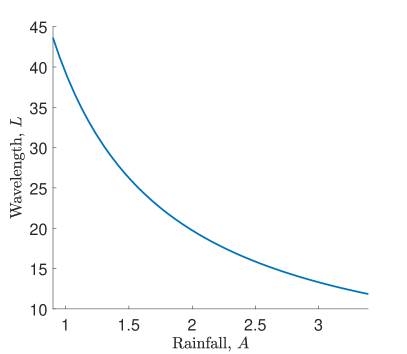
(a)

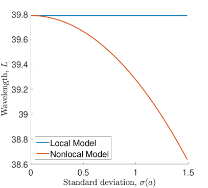
(b)

Figure 2.1: Variation in pattern wavelength with rainfall $A$ and standard deviation $\sigma(a)$. Part (a) shows the wavelength (2.7) of the patterns as it decreases with the rainfall $A$ for nonlocal model. The parameter values are $B=0.45$, $\nu=182.5$, $C=1$ and $a=1$. Part (b) compares the wavelength predicted from the nonlocal model with the setting $C=a^{2}$ as it varies with the dispersal parameter $a$ and compares it to the wavelength obtained from the local model. It shows that the nonlocal model predicts a shorter distance between the vegetation stripes, especially if the shape of the dispersal kernel is wide. However, the difference is very small (see the $y$-axis of the plot). The parameter values used for this are $A=1$, $B=0.45$, $\nu=182.5$

3 Travelling Wave Solutions

The constant uphill migration of the vegetation patterns suggests considering travelling waves. In this section we will investigate the travelling wave form of the nonlocal Klausmeier model (1.2). Pattern solutions of the original PDE model then correspond to periodic solutions of the travelling wave ODEs. From the equations in their travelling wave form we will not only be able to confirm the results on the maximum rainfall supporting pattern formation obtained by performing linear stability analysis in Section 2, but also deduce more information about the migration speed of the patterns. The nature of the patterned solutions fundamentally depends on the scaling of the migration speed $c$. The highest rainfall level supporting pattern formation occurs for $c=O_{s}(1)$. For this situation we determine conditions for Hopf bifurcations to occur; for the local Klausmeier model (1.1) the parameter range in the $A$-$c$ plane that supports pattern formation is bounded above by the locus of a Hopf bifurcation [54], and we anticipate the same for the nonlocal model.

Applying the travelling wave ansatz $u(x,t)=U(z)$, $w(x,t)=W(z)$, $z=x-ct$ to the nonlocal model (1.2), gives

$$\frac{{\operatorname{d}}U}{{\operatorname{d}}z} =-\frac{1}{c}\left(U^{2}W-BU+C\left(\int_{-\infty}^{\infty}\phi(z-z^{\prime})U(z^{\prime}){\operatorname{d}}z^{\prime}-U(z)\right)\right),$$

$$\frac{{\operatorname{d}}W}{{\operatorname{d}}z} =-\frac{1}{c+\nu}\left(A-W-U^{2}W+d\frac{{\operatorname{d}}^{2}W}{{\operatorname{d}}z^{2}}\right).$$

To investigate the occurrence of a Hopf bifurcation, consider perturbations $\tilde{U}(z)$, $\tilde{W}(z)$ proportional to $e^{\lambda z}$ of the steady state $(\overline{U},\overline{W})=(\overline{u},\overline{w})$. Setting $\phi$ to be the Laplacian kernel (1.4) and linearising the resulting system gives that $\lambda$ satisfies

$$\lambda^{5}+\alpha\lambda^{4}+\beta\lambda^{3}+\gamma\lambda^{2}+\delta\lambda+\varepsilon=0,$$ (3.1)

where

$$\alpha =\frac{d(B-C)+c(c+\nu)}{cd},$$

$$\beta =\frac{-2B^{2}\left(a^{2}cd-(B-C)(c+\nu)\right)-Ac\left(A+\sqrt{A^{2}-4B^{2}}\right)}{2B^{2}cd},$$

$$\gamma =\frac{-2B^{2}a^{2}\left(d+c(c+\nu)\right)+A(B+C)\left(A+\sqrt{A^{2}-4B^{2}}\right)-4B^{3}}{2B^{2}cd},$$

$$\delta =\frac{a^{2}\left(-2B^{3}(c+\nu)+Ac\left(A+\sqrt{A^{2}-4B^{2}}\right)\right)}{2B^{2}cd},$$

$$\varepsilon =\frac{a^{2}\left(-A\left(A+\sqrt{A^{2}-4B^{2}}\right)+4B^{2}\right)}{2B^{2}cd}.$$

To find conditions for a Hopf bifurcation to occur, set $\lambda=i\omega$, $\omega\in\mathbb{R}$. This splits (3.1) into its real and imaginary parts, which after solving for and eliminating $\omega^{2}$ gives the condition

$$\frac{\gamma\pm\sqrt{\gamma^{2}-4\alpha\varepsilon}}{2\alpha}=\frac{\beta\pm\sqrt{\beta^{2}-4\delta}}{2}.$$ (3.2)

The assumption $\omega\in\mathbb{R}$ requires that the left and right hand sides of this equation are both positive. This leads to an additional condition (3.5) that will be considered later. To further investigate (3.2), we expand it in $1/\nu$. This gives

$$\frac{((B-C)\operatorname{sign}(c)+B+C)a^{2}}{B-C}+O\left(\frac{1}{\nu}\right)=0.$$

For the first term of the expansion to be zero, one would require $B>C$ with one of the parameters being equal to zero, depending on the sign of $c$. This is, however, not possible due to the positivity assumptions on the parameters. Investigating the next term of the expansion suggests using the scaling $A=O_{s}(\nu^{1/2})$. Applying this scaling to (3.2), expanding in $\nu\gg 1$ and then solving for $c$ shows that a Hopf bifurcation exists at

$$c_{\pm}=\left(\frac{B}{2A^{2}}+\frac{A^{2}(2B-C)}{2\left(-B^{4}a^{2}\nu^{2}+A^{4}\right)}\right.\\ \pm\left.\left(\frac{B^{2}}{4A^{4}}+\frac{3BC}{2\left(-B^{4}a^{2}\nu^{2}+A^{4}\right)}+\frac{4B^{6}a^{2}\nu^{2}-4A^{4}BC+A^{4}C^{2}}{4\left(-B^{4}a^{2}\nu^{2}+A^{4}\right)^{2}}\right)^{\frac{1}{2}}\right)\nu B^{2},$$ (3.3)

to leading order in $\nu$ as $\nu\rightarrow\infty$. Since the migration speed $c\in\mathbb{R}$, this requires

$$A<A_{\max}=\left(\frac{3C-B-2\sqrt{2C}\sqrt{C-B}}{\left(B+C\right)^{2}}\right)^{\frac{1}{4}}a^{\frac{1}{2}}B^{\frac{5}{4}}\nu^{\frac{1}{2}},$$ (3.4)

and $C>B$. This is the same condition as (2.5) obtained in Section 2.

In deriving this condition we assumed that the terms in (3.2) were positive. By applying the scaling $A=O_{s}(\nu^{1/2})$ and expanding in $\nu\gg 1$, this yields the bounds

$$\max\left\{0,\frac{B^{2}(B-C)\nu}{A^{2}}\right\}<c<\frac{B^{3}\nu}{A^{2}},$$ (3.5)

to leading order in $\nu$. This condition is satisfied if $C>B$. In the case of $C=a^{2}$ it holds if $a>\sqrt{B}$.

Setting $C=a^{2}$ and taking the limit $a\rightarrow\infty$ in both (3.3) and (3.4) gives, as expected by the considerations on the limiting behaviour of the model, the corresponding conditions obtained by [52] for the local model. Further the right hand side of (3.4) is decreasing for all $a>\sqrt{B}$ in the setting $C=a^{2}$. Combined with the observation that it approaches the corresponding condition for the local model as $a\rightarrow\infty$, this shows that pattern formation is more likely in the nonlocal model with the tendency to form patterns increasing as the dispersal parameter $a$ decreases, i.e. as the width of the kernel $\phi$ increases. Figure 3.1a shows this for some fixed parameter values.

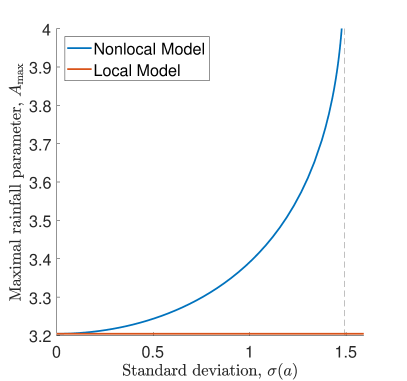
(a)

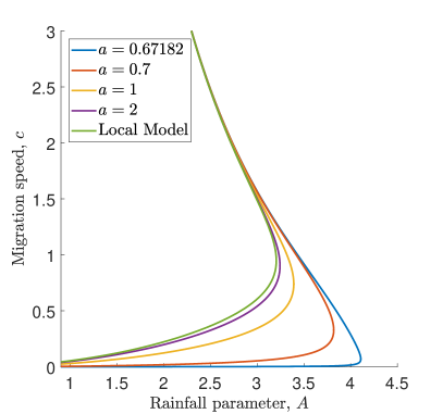
(b)

Figure 3.1: Variation in the loci of the Hopf bifurcation and maximum rainfall parameter $A_{\max}$ with kernel width in the case $C=a^{2}$. The plot in (a) compares the upper bound (2.5) on the rainfall parameter $A$ of the nonlocal model using the Laplacian kernel with $C=a^{2}$ with condition (2.6) obtained for the local model. Note that one requires $a>\sqrt{B}$ for $A_{\max}\in\mathbb{R}$ in the case of the nonlocal model. Part (b) compares the loci (3.3) of the Hopf bifurcations of the nonlocal model for different values of the dispersal parameter $a$ to the locus of the local model obtained by [52]. The parameter values used in both figures are $B=0.45$, $\nu=182.5$

Finally, Figure 3.1b combines these considerations by showing the loci (3.3) of the Hopf bifurcations of the nonlocal model for different values of the dispersal parameter $a$ in the $A$-$c$ plane and compares it to the corresponding locus of the local model. As shown previously, this implies that in the nonlocal model a larger parameter region supports pattern formation, especially as the dispersal parameter $a$ is decreased, i.e. as the width of the kernel is increased. This means that the nonlocal model predicts that plants which disperse their seeds over a larger distance will undergo a change from homogeneous vegetation to patterns at a higher level of rainfall than those plants with a narrower and diffusion-like dispersal, as the amount of rainfall is gradually decreased.

If $C\neq a^{2}$, it is not appropriate to compare the nonlocal model to the local model. However, one can still investigate how a change in the dispersal parameter $a$ affects the tendency to form patterns in this situation. We will first consider the case in which $C$ is constant. In this situation (3.4) yields that the highest rainfall parameter supporting pattern formation $A_{\max}$ is proportional to $a^{1/2}$. This means that if the dispersal kernel gets narrower, a larger range of the rainfall parameter $A$ supports pattern formation. This is visualised in Figure 3.2a, which shows the maximum rainfall parameter $A_{\max}$ plotted against the dispersal parameter $a$ and in Figure 3.2b, which visualises the location of the Hopf bifurcation (3.3), where $C$ is constant. This is contrary to the behaviour observed in the case of $C=a^{2}$, where a narrower kernel gave less tendency to form patterns.

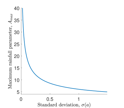
(a)

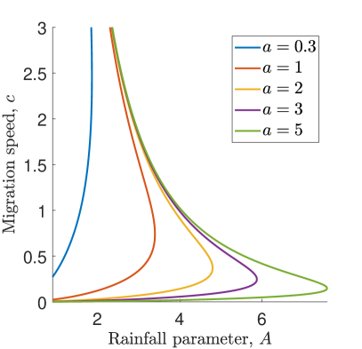
(b)

Figure 3.2: Variation in the loci of the Hopf bifurcation and maximum rainfall parameter $A_{\max}$ with kernel width in the case of constant $C$. The plot in (a) shows how upper bound $A_{\max}$ given in (3.4) of the rainfall parameter $A$ that supports pattern formation in the nonlocal model using the Laplacian kernel varies as the dispersal parameter $a$ is changed. Here $C=1$ is fixed. Part (b) shows the loci (3.3) of the Hopf bifurcations of the nonlocal model with the Laplacian kernel for different values of the dispersal parameter $a$, where the dispersal coefficient $C$ is constant. The parameter values used here are $B=0.45$, $C=1$, $\nu=182.5$

Investigating the final case, i.e. the one of fixed $a$ and varying $C$, shows that the critical rainfall parameter $A_{\max}$ is decreasing with increasing $C$ for all $C>B$. This shows that the more the plants invest in their dispersal, the less likely is the formation of patterns. Similar to the previous two cases, the change in $A_{\max}$ is visualised in Figure 3.3a and the loci of the Hopf bifurcations in the $A$-$c$ plane is shown in Figure 3.3b.

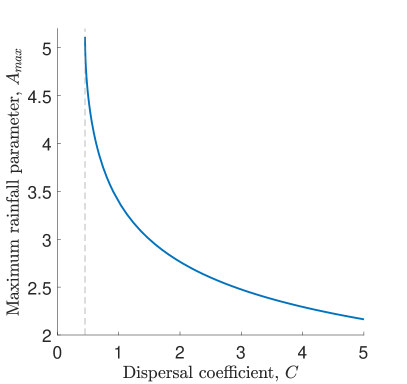
(a)

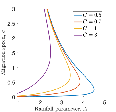
(b)

Figure 3.3: Variation in the loci of the Hopf bifurcation and maximum rainfall parameter $A_{\max}$ with kernel width in the case of constant $a$. The plot in (a) shows how upper bound $A_{\max}$ given in (3.4) of the rainfall parameter $A$ that supports pattern formation in the nonlocal model with Laplacian kernel varies as the dispersal coefficient $C$ is changed. Here $a=1$ is fixed. Note that $C>B$ is required for $A_{\max}\in\mathbb{R}$. Part (b) shows the loci (3.3) of the Hopf bifurcations in the same situation. The parameter values used here are $B=0.45$, $C=1$, $\nu=182.5$

4 Asymptotic Analysis of the Integro-PDE Model

In the previous sections we have applied different techniques to the model (1.2) to find conditions for pattern formation in their leading order form. In this section we will confirm these by first obtaining the leading order form of the Integro-PDE model and then deducing conditions for Hopf bifurcations from it.

Applying the rescalings $u=AB^{-1}u^{*}$, $w=A^{-1}B^{2}w^{*}$, $t=B^{-1}t^{*}$, $c=Bc^{*}$, $\nu=A^{2}B^{-2}\Gamma^{-1}$, $B^{-1}C=D$ to (1.2) gives

$$\frac{\partial u}{\partial t} =u^{2}w-u+D\left(\int_{-\infty}^{\infty}\phi(x-y)u(y,t){\operatorname{d}}y-u(x,t)\right),$$

$$B\nu^{-1}\frac{\partial w}{\partial t} =\Gamma\left(1-u^{2}w\right)-\nu^{-1}w+\frac{\partial w}{\partial x}+d\nu^{-1}\frac{\partial^{2}w}{\partial x^{2}},$$

where the ^∗’s were dropped for brevity. Again assuming that $A=O_{s}(\nu^{1/2})$, the leading order form in $\nu$ of this is

$$\frac{\partial u}{\partial t} =u^{2}w-u+D\left(\int_{-\infty}^{\infty}\phi(x-y)u(y,t){\operatorname{d}}y-u(x,t)\right),$$

$$0 =\Gamma\left(1-u^{2}w\right)+\frac{\partial w}{\partial x}.$$

Applying the travelling wave ansatz $u(x,t)=U(z)$, $w(x,t)=W(z)$, $z=x-ct$, gives

$$-c\frac{{\operatorname{d}}U}{{\operatorname{d}}z} =U^{2}W-U+D\left(\int_{-\infty}^{\infty}\phi(z-z^{\prime})U(z^{\prime}){\operatorname{d}}z^{\prime}-U(z)\right),$$

$$0 =\Gamma\left(1-U^{2}W\right)+\frac{{\operatorname{d}}W}{{\operatorname{d}}z}.$$

This system has a unique steady state given by $(\overline{U},\overline{W})=(1,1)$. Consider small perturbations $\tilde{U}$, $\tilde{W}$ of the steady state that are proportional to $e^{\lambda z}$. Letting $\phi$ to be the Laplacian kernel (1.4) and linearising the resulting system yields that $\lambda$ satisfies

$$\lambda^{4}+\overline{\alpha}\lambda^{3}+\overline{\beta}\lambda^{2}+\overline{\gamma}\lambda+\overline{\delta}=0,$$ (4.1)

where

$$\overline{\alpha}=\frac{1-D-\Gamma c}{c},\quad\overline{\beta}=\frac{\Gamma(1-D)-a^{2}c}{c},\quad\overline{\gamma}=\frac{a^{2}(\Gamma c-1)}{c},\quad\overline{\delta}=-\frac{\Gamma a^{2}}{c}.$$

To find conditions for a Hopf bifurcation to occur, again set $\lambda=i\omega$, $\omega\in\mathbb{R}$. Analogous to the preceding sections, this allows splitting (4.1) into its real and imaginary parts, which after solving for $\omega^{2}$, assuming that $\omega\neq 0$, gives

$$\frac{\overline{\beta}\pm\sqrt{\overline{\beta}^{2}-4\overline{\delta}}}{2}=\frac{\overline{\gamma}}{\overline{\alpha}},$$ (4.2)

as the leading order condition for a Hopf bifurcation to occur. The restriction $\omega\in\mathbb{R}$, implies the additional requirement

$$\max\left\{0,\frac{1-D}{\Gamma}\right\}<c<\frac{1}{\Gamma}.$$ (4.3)

If $c>0$, then $\overline{\delta}<0$ and thus one needs to choose the plus sign on the left hand side in (4.2). Solving for $c$ gives

$$c_{\pm}={\frac{\left(D-3\right){\Gamma}^{2}+{a}^{2}\pm\sqrt{\left(D+1\right)^{2}{\Gamma}^{4}-2{a}^{2}\left(3D-1\right){\Gamma}^{2}+{a}^{4}}}{2{\Gamma}\left({a}^{2}-\Gamma^{2}\right)}}.$$ (4.4)

To satisfy (4.3), one requires $C>B$ and

$$\Gamma<\left(\frac{3D-1+2\sqrt{2D(D-1)}}{(D+1)^{2}}\right)^{\frac{1}{2}}a.$$ (4.5)

Therefore, the steady state $(\overline{U},\overline{W})=(1,1)$ undergoes a Hopf bifurcation if (4.3), (4.4) and (4.5) are satisfied. Substituting the rescalings used at the beginning of this section into these three conditions gives the same conditions (3.5), (3.3) and (3.4) that were obtained form the travelling wave equations in Section 3.

5 Numerical Simulations

So far, we have only considered one particular form of dispersal kernel in the nonlocal Klausmeier model (1.2). In this section we will solve the model numerically for different kernel functions and use the solutions to estimate the maximum rainfall parameter giving patterns for each kernel. The simulations will show that the parametric trends that were obtained for the Laplacian kernel carry over to other kernel functions, i.e. a wider dispersal kernel and a higher dispersal rate decrease the tendency to form patterns, while under the assumption that $C=2/\sigma(a)^{2}$, an increase in kernel width causes an increase in the size of the parameter region giving patterns. Our numerical simulations will further show that the tendency to form patterns depends on the type of decay of the dispersal kernel.

In the analysis performed in previous sections, we considered the model on an infinite domain. To mimic this in the simulations, we will consider a subdomain centred in a larger domain with the following initial conditions; outside the smaller subdomain the system’s initial state will be set to the steady state, while on the subdomain a random perturbation will be added. The idea of this is to choose the outer domain large enough so that any conditions imposed on the boundary of this domain (which are set to be periodic in our simulations) do no affect the solution on the inner subdomain in the finite time that is considered in the simulation. The solution is then only considered on the subdomain on which a perturbation was introduced. To solve the Integro-PDE system (1.2), it is first transformed into an ODE system by discretising its space domain and then solved by the built-in MATLAB ODE solver ode15s. A significant simplification is made by computing the convolution term using the fast Fourier transform, as it reduces the number of operations required to find the convolution from $O(M^{2})$ to $O(M\log(M))$ in each step (e.g. [8]), where $M$ is the number of points of the space domain. Figure 5.1 shows typical solutions obtained by this method; in Figure 5.1a the rainfall was chosen large enough for the solution to converge to the steady state, while for Figure 5.1b parameters that produce a patterned solution of the nonlocal Klausmeier model using the Laplacian kernel were used.

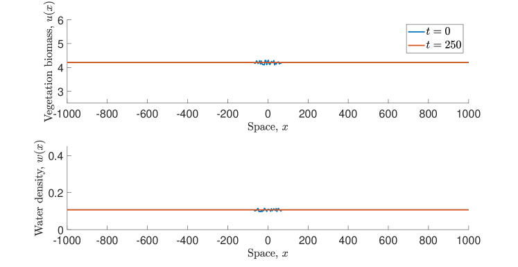
(a)

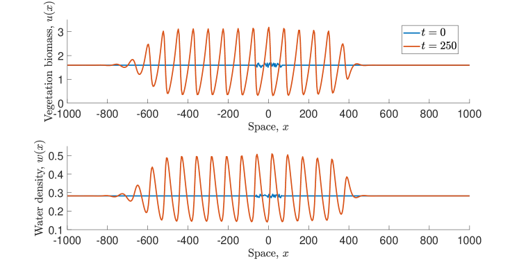
(b)

Figure 5.1: Numerical solution of the nonlocal Klausmeier model (1.2) using the Laplacian kernel (1.4) for different rainfall levels. In (a) $A=2$ yields convergence to the coexisting steady state from which the system is perturbed initially. Part (b) displays a patterned solution obtained by setting $A=1$. The other parameter values used in both simulations are $B=0.45$, $\nu=50$, $d=100$, $a=2$, $C=4$ and the number of space points is $M=2^{9}$

Using these simulations, we set up a scheme, based on the amplitude of the oscillation of the solution of the nonlocal Klausmeier model (1.2) relative to the steady state that approximates the critical rainfall parameter $A_{\max}$, that is the maximum rainfall parameter supporting pattern formation, for different kernel functions $\phi(x)$. Unlike in the simulation results shown in Figure 5.1, we run the simulations over a shorter amount of time (up to $t=30$), as we are only interested in the onset of spatial patterns rather than in any of their properties. The kernel functions used in our simulations are those introduced in Section 1, i.e. the Laplacian (1.4), the Gaussian (1.5) and the power law kernel (1.6). Note that the standard deviations $\sigma(a)$ are given by $\sigma(a)=\sqrt{2}/a$ for the Laplacian kernel, $\sigma(a_{g})=1/(\sqrt{2}\,a_{g})$ for the Gaussian kernel and $\sigma(a_{p})=\sqrt{2}/(\sqrt{b^{2}-5b+6}\,a_{p})$ for the power law kernel, provided $b>3$. If the shape parameter of the power law kernel is $b\leq 3$, its standard deviation is infinite and a meaningful comparison to other kernel functions cannot be performed based on their standard deviations. In our simulations we consider both $b=3.1$ and $b=4$. As in previous sections, we will consider the case in which $C=2/\sigma(a)^{2}$, motivated by the limiting behaviour of the nonlocal model, and the cases in which either $C$ or $a$ is assumed to be constant and the other parameter is varied.

Figure 5.2a shows the results of our simulations in the case of $C$ being constant. The trend that a narrower dispersal kernel requires a higher level of rainfall to form homogeneous vegetation, which was predicted by the leading order form (3.4) of $A_{\max}$ for the Laplacian kernel, carries over to the other kernels used in the simulations. Further one can observe that the power law distributions which have algebraic decay give a larger value of $A_{\max}$ than those with exponential decay if the standard deviation is sufficiently large ($\sigma(a)\gtrapprox 0.3$), while for narrower kernels the opposite is true. While the results of our simulations for the Laplacian kernel and the corresponding leading order form of $A_{\max}$ fit well for sufficiently large values of the standard deviation $\sigma(a)$, the fit is poorer for narrower kernel functions (see Figure 5.2b for a comparison). The reason for this is the relatively small choice of $\nu=50$, which was taken to improve the speed of the simulations. Solutions for larger $\nu$ indicate that the relative difference between $A_{\max}$ in our simulations and in the analytical approximation decreases (slowly) with increasing $\nu$.

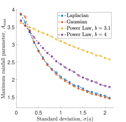
(a)

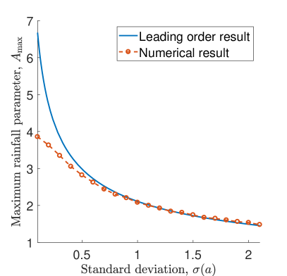
(b)

Figure 5.2: Illustration of the results of our numerical scheme to approximate the maximum rainfall parameter $A_{\max}$ in the case of constant $C$. Part (a) shows the results of our simulations in the case of $C$ being constant. We have determined the maximum rainfall parameter giving patterns for the Laplacian kernel (1.4), the Gaussian kernel (1.5) and the power law kernel (1.6) for both $b=3.1$ and $b=4$, at $\sigma(a)=\{0.1,0.2,\dots 2.1\}$. The parameter values used in these simulations are $B=0.45$, $C=1$, $\nu=50$, $d=1$. Part (b) compares the simulation results obtained for the Laplacian kernel to the corresponding condition (3.4) valid to leading order in $\nu$

We repeat the same scheme in the setting of $C=2/\sigma(a)^{2}$ for the same kernel functions. The results of this are shown in Figure 5.3. Considering the type of decay of the kernel functions, the results of it are similar to the simulations of the case of $C$ being constant. One can observe that the distributions with algebraic decay yield a larger value of $A_{\max}$ than the distributions with exponential decay if the kernel is sufficiently wide, while for narrow kernels the opposite is true. Further, considering one specific kernel on its own, a narrower dispersal kernel now gives a lower value of the maximum rainfall parameter supporting pattern formation. This is in contrast to the case in which $C$ was kept constant but in accord with the leading order form (3.4) of $A_{\max}$. As before, it can also be observed from the simulations of the model using the Laplacian kernel that for the choice of $\nu=50$, the numerical simulations are a good approximation of the leading order result only for sufficiently wide kernels.

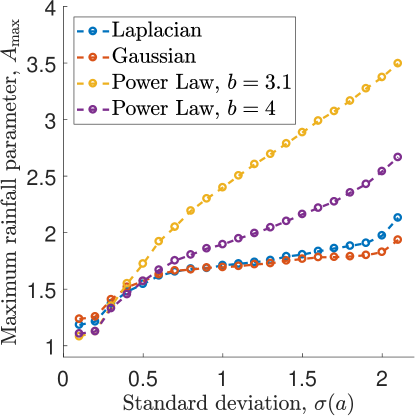
Figure 5.3: Illustration of the results of our numerical scheme to approximate the maximum rainfall parameter $A_{\max}$ in the case of $C=2/\sigma(a)^{2}$. We have considered the Laplacian kernel (1.4), the Gaussian kernel (1.5) and the power law kernel (1.6) for both $b=3.1$ and $b=4$ and determined the value of the maximum rainfall parameter giving patterns $A_{\max}$ at $\sigma(a)=\{0.1,0.2,\dots 2.1\}$ for each kernel function in the case of $C=2/\sigma(a)^{2}$. The parameters used in this simulation are $B=0.45$, $\nu=50$, $d=1$

Finally, we apply the same scheme to the case of fixed dispersal parameter $a$ and varying dispersal coefficient $C$ (Figure 5.4). As in the previous cases, the trends of the simulations of other kernel functions are again in alignment with the leading order result (3.4) for the Laplacian kernel. An increase in dispersal rate $C$ causes a decrease in $A_{\max}$ for each of the dispersal kernels considered in our simulations. Further, the comparison of kernels with algebraic and exponential decay depends on the choice of standard deviation $\sigma(a)$, as indicated by the previous simulations in which the standard deviation was varied. Figure 5.4b shows that for a small standard deviation ($\sigma(a)=0.2$ in this case), the kernels with exponential decay predict that a higher level of rainfall is required to form a uniform vegetation cover than those with algebraic decay. If the standard deviation is sufficiently large, the opposite trend is observed. This is visualised in Figure 5.4a, where the standard deviation was set to $\sigma(a)=1$.

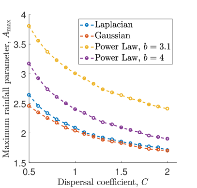
(a)

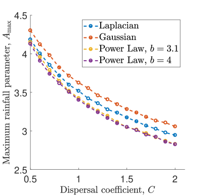
(b)

Figure 5.4: Illustration of the results of our numerical scheme to approximate the maximum rainfall parameter $A_{\max}$ in the case of constant $a$. We have considered the Laplacian kernel (1.4), the Gaussian kernel (1.5) and the power law kernel (1.6) for both $b=3.1$ and $b=4$ and determined the value of the maximum rainfall parameter giving patterns $A_{\max}$ at $C=\{0.5,0.6,\dots 2\}$ for each kernel function, with $a$ being fixed. In (a), the standard deviation was chosen as $\sigma(a)=1$, in (b) as $\sigma(a)=0.2$. The other parameters used in this simulation are $B=0.45$, $\nu=50$, $d=1$

6 Discussion

The main results of this paper are given by (3.3) and (3.5), which give an upper bound for the parameter region in the $A$-$c$ plane supporting pattern formation, valid to leading order in $\nu$, for the nonlocal Klausmeier model (1.2) with the Laplacian kernel (1.4). In particular this gives the upper bound $A_{\max}$, defined in (3.4), on the rainfall parameter, again valid to leading order in $\nu$. In other words, $A_{\max}$ represents the lowest level of rainfall that allows plants to form a homogeneous vegetation cover, while lower amounts of water only support banded vegetation. These results hold under the assumptions that the migration speed $c$ is $O_{s}(1)$ and that the parameter region supporting pattern formation is bounded above by the loci of Hopf bifurcations, which was shown by [54] for the local Klausmeier model (1.1). While the simple nature of the Klausmeier model makes it impossible to deduce any quantitative conclusions from these results, they do give a good insight into the parametric trends of the model. These trends fundamentally depend on the assumption made on the factor $C$ scaling the convolution term in the nonlocal model.

In this paper we considered three different cases of the coefficient $C$ in the nonlocal Klausmeier model; that of choosing it to be constant, the one of varying $C$ for fixed dispersal parameter $a$ and that of setting $C=2/\sigma(a)^{2}$. In the case of $C$ being fixed, a change in the dispersal parameter $a$ only affects the width of the dispersal kernel, but leaves the term scaling the nonlocal plant dispersal term unchanged. It can be immediately concluded from (3.4) that the threshold $A_{\max}$ increases as the kernel width decreases. This increase in the size of the parameter region supporting pattern formation is also visualised in Figure 3.2b. This means that the wider plants disperse their seeds, the less water they require to form a homogeneous vegetation cover. In particular, our results show that if plant dispersal is wide enough, the location of the Hopf bifurcation bounding the pattern forming parameter region completely lies in the region that only supports the trivial steady state describing complete desertification. In this case, the assumptions taken in this paper predict that no striped vegetation can occur. Plants either form a homogeneous vegetation cover or disappear completely.

The expression given by (3.4) is only valid for the Laplacian kernel (1.4) and to leading order in $\nu$. The numerical simulations in Section 5 allow us to compare this condition to those for other kernel functions that have been suggested by studies on plant dispersal (see [7] for an overview). Our results suggest that the maximum rainfall level giving patterned vegetation depends on the width and therefore also on the type of decay of the dispersal kernel. It can be seen from Figures 5.2a and 5.3 that those probability distributions that decay algebraically predict a larger pattern-giving parameter region for some fixed standard deviation than those decaying exponentially under all the different assumptions taken on $C$ in this paper, if the dispersal kernel is sufficiently wide. If the kernel is narrow, the opposite behaviour is observed. Further, the simulations show that $A_{\max}$ for each individual kernel is decreasing as the width of the kernel is increased if one assumes that $C$ is constant. This is in accord with the behaviour of the leading order form (3.4) of the Laplacian kernel. Combining these observations, we can conclude that the narrower a plant’s seed dispersal is, the more water is required to avoid the formation of patterns. Nevertheless, field data shows that plants in semi-arid ecosystems tend to establish narrow dispersal kernels [13, 62]. This is, however, only a side effect of other adaptations such as seed containers protecting seeds from flooding and predation [13]. Simulations show that short range dispersal yields a higher mean biomass in those ecosystems than a long distance spread of seeds [39]. Combining this with the results of this paper shows that the shortening of dispersal ranges of plants in semi-arid environments increases their tendency to self-organise into patterns.

If one assumes that the width of the dispersal kernel is fixed and plant’s dispersal rate is changed, (3.4) shows that, under the assumption that the dispersal of seeds fits the Laplacian kernel, the more the species invests in its dispersal rate, the less water it requires to form a homogeneous vegetation cover. For the other dispersal kernels we have considered, the same behaviour is shown in our simulations. Those simulations also show the same trend regarding the type of decay of the dispersal kernels as the simulations in the case of fixed $C$ and varying range of dispersal. For wider dispersal kernels, those plants whose kernel functions decay algebraically have a higher tendency to form patterns than those plants dispersing their seeds according to an exponentially decaying kernel. For sufficiently narrow kernels, the opposite observation can be made.

The final choice of $C$ assumes that it is correlated with the standard deviation of the dispersal kernel as $C=2/\sigma(a)^{2}$. This choice is of particular significance because it leads to the local Klausmeier model being a limiting case of the nonlocal model using either the Laplacian or the Gaussian kernel. This allows us to compare our results to the corresponding results obtained for the local model by [52]. This choice is motivated purely mathematically and we are not aware of any evidence that the dispersal coefficient $C$ is correlated with the seed distribution range in such a way. However, experiments have shown that plants’ rate of dispersal increases in semi-arid environments [2], e.g. by the production of more but smaller seeds [63] as well as that plants develop short range dispersal of seeds [13, 62]. The analysis of the previous two cases has shown that an increase in the dispersal coefficient reduces the critical level of rainfall required to form a homogeneous vegetation cover, while the establishment of a narrow dispersal kernel increases this threshold. Therefore, this could be seen as an evolutionary trade-off.

The leading order results on quantities such as $A_{\max}$ or the wavelength, obtained in Sections 2 and 3, resemble the limiting behaviour of this case. Apart from the limiting case, the results for the nonlocal model using the Laplacian kernel behave monotonically as the width of the dispersal kernel is changed. In particular, the results on the loci of the Hopf bifurcation and the maximum rainfall parameter giving patterns allow us to make the crucial observation that the nonlocal model predicts a larger range of parameters supporting pattern formation. Our results further show that the size of the parameter region giving patterns is larger for a wider dispersal kernel, which makes the dispersal term less influential, i.e. it decreases the plant’s dispersal rate, due to the assumption $C=a^{2}$. This is most strikingly illustrated by Figure 3.1b, which shows the increase of this region as the scale parameter $a$ of the kernel decreases. Under this assumption on the dispersal rate and the kernel width, our simulation results show that establishing short range dispersal increases plants’ ability to form a homogeneous vegetation cover. This is further illustrated by Figure 6.1, which shows shows the contours of $A_{\max}$ and the suggested evolutionary trade-off $C=2/\sigma(a)^{2}$. The latter crosses the contours as the standard deviation is varied and thereby shows that an increase in kernel width yields an increase in the maximum rainfall parameter supporting pattern formation.

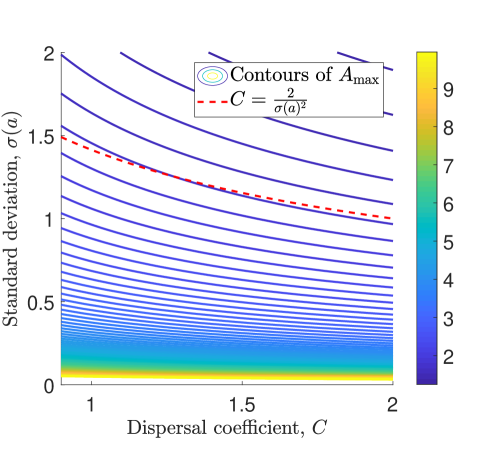
Figure 6.1: Contour plot of $A_{\max}$. This plot shows the contours of (3.4) as solid lines with the colours indicating the level of $A_{\max}$. The red dotted line is the suggested trade-off $C=2/\sigma(a)^{2}$, which was mathematically motivated by the limiting behaviour of the convolution integral

In this paper we have also investigated the distance between the striped vegetation patches to leading order in $\nu$. It is of immense importance to have an understanding of the wavelength of the patterns as it might give an indication of whether the ecosystem is close to complete desertification. The results of this study show that the wavelength monotonically increases as the amount of rainfall decreases, before reaching a critical threshold, where patterns disappear and complete desertification takes over. While it is important to emphasise again that the simplifications assumed in deducing the Klausmeier model do not allow us to gain any quantitative information, we have shown how the wavelength is affected by changes in the width of the dispersal kernel or in the plant’s dispersal rate. Interestingly, in the case of $C=2/\sigma(a)^{2}$, the wavelength predicted by the nonlocal model using the Laplacian kernel does not differ much from the wavelength predicted by the local model, even for wide dispersal kernels (see the $y$-axis in Figure 2.1b). This suggests that one could make predictions on the possibility of desertification without having any information on the range of plant dispersal under the assumption that the dispersal coefficient $C$ is correlated with the standard deviation of the dispersal kernel in such a way.

The pattern solutions of the Klausmeier model fundamentally depend on how the migration speed $c$ scales with the parameter $\nu$, describing the rate of the water flow downhill. In this paper we have only considered the case $c=O_{s}(1)$ and the patterns forming in the vicinity of the Turing-Hopf bifurcation. For the local Klausmeier model results have been obtained for a wide range of migration speeds [49, 50, 51, 52, 53]. One natural extension of this work would be to do a similar comprehensive study of the whole parameter range for the nonlocal model. This would give insights into the existence and form of patterns away from the bifurcation point.

Another natural area for future work would be to consider other more realistic models for vegetation patterns. A number of such models and their underlying mechanisms and scale dependent feedbacks are reviewed by [31]. Some of these models already include nonlocal dispersal via convolution integrals [3, 39, 40], and in others [18, 41] such a term could be added in place of plant diffusion. While these as well as the model considered in this paper assume an isotropic dispersal of plants, this simplification can be removed by including either advection of plants [57, 46] or an asymmetric dispersal kernel [57]. Similar to the relation between diffusion and the convolution with a symmetric kernel, both the advection and the diffusion terms arise from the convolution term with an asymmetric kernel. In this case the coefficient of the first order derivative in (1.3) is non-zero. Finally, some models use a nonlocal term for the water uptake and thus also for plant growth, reflecting the extensive root networks of plants in semi-arid regions [14, 15]. Investigation of these models using an approach similar to that in the current paper would be of interest but would be particularly challenging because of the added complexity.

References

- [1] E. J. Allen, L. J. S. Allen, and X. Gilliam. Dispersal and competition models for plants. J. Math. Biol., 34(4):455–481, 1996. 10.1007/BF00167944.
- [2] J. Aronson, J. Kigel, and A. Shmida. Reproductive allocation strategies in desert and mediterranean populations of annual plants grown with and without water stress. Oecologia, 93(3):336–342, 1993. 10.1007/BF00317875.
- [3] M. Baudena and M. Rietkerk. Complexity and coexistence in a simple spatial model for arid savanna ecosystems. Theor. Ecol., 6(2):131–141, 2013. 10.1007/s12080-012-0165-1.
- [4] F. Borgogno, P. D’Odorico, F. Laio, and L. Ridolfi. Mathematical models of vegetation pattern formation in ecohydrology. Rev. Geophys., 47:RG1005, 2009. 10.1029/2007RG000256.
- [5] N. F. Britton. Spatial structures and periodic travelling waves in an integro-differential reaction-diffusion population model. SIAM J. Appl. Math., 50(6):1663–1688, 1990. 10.1137/0150099.
- [6] J. Bromley, J. Brouwer, A. Barker, S. Gaze, and C. Valentine. The role of surface water redistribution in an area of patterned vegetation in a semi-arid environment, south-west Niger. J. Hydrol., 198(1):1 – 29, 1997. 10.1016/S0022-1694(96)03322-7.
- [7] J. M. Bullock, L. M. González, R. Tamme, L. Götzenberger, S. M. White, M. Pärtel, and D. A. P. Hooftman. A synthesis of empirical plant dispersal kernels. J. Ecol., 105(1):6–19, 2017. 10.1111/1365-2745.12666.
- [8] J. W. Cooley, P. A. W. Lewis, and P. D. Welch. The fast Fourier transform and its applications. IEEE Trans. Educ., 12(1):27–34, 1969. 10.1109/TE.1969.4320436.
- [9] A. Cornet, J. Delhoume, and C. Montaña. Dynamics of striped vegetation patterns and water balance in the Chihuahuan Desert, pages 221–231. SPB Academic Publishing, The Hague, 1988.
- [10] C. Cosner, J. Dávila, and S. Martínez. Evolutionary stability of ideal free nonlocal dispersal. J. Biol. Dyn., 6(2):395–405, 2012. 10.1080/17513758.2011.588341. PMID: 22873597.
- [11] V. Deblauwe. Modulation des structures de végétation auto-organisées en milieu aride, 2010.
- [12] D. Dunkerley and K. Brown. Oblique vegetation banding in the Australian arid zone: implications for theories of pattern evolution and maintenance. J. Arid. Environ., 51(2):163 – 181, 2002. 10.1006/jare.2001.0940.
- [13] S. Ellner and A. Shmida. Why are adaptations for long-range seed dispersal rare in desert plants? Oecologia, 51(1):133–144, 1981. 10.1007/BF00344663.
- [14] E. Gilad, J. von Hardenberg, A. Provenzale, M. Shachak, and E. Meron. Ecosystem engineers: From pattern formation to habitat creation. Phys. Rev. Lett., 93:098105, 2004. 10.1103/PhysRevLett.93.098105.
- [15] E. Gilad, J. von Hardenberg, A. Provenzale, M. Shachak, and E. Meron. A mathematical model of plants as ecosystem engineers. J. Theor. Biol., 244(4):680 – 691, 2007. j.jtbi.2006.08.006.
- [16] S. A. Gourley, M. A. J. Chaplain, and F. A. Davidson. Spatio-temporal pattern formation in a nonlocal reaction-diffusion equation. Dyn. Syst., 16(2):173–192, 2001. 10.1080/14689360116914.
- [17] C. F. Hemming. Vegetation arcs in Somaliland. J. Ecol., 53(1):57–67, 1965. 10.2307/2257565.
- [18] R. HilleRisLambers, M. Rietkerk, F. van den Bosch, H. H. T. Prins, and H. de Kroon. Vegetation pattern formation in semi-arid grazing systems. Ecology, 82(1):50–61, 2001. 10.2307/2680085.
- [19] V. Hutson, S. Martinez, K. Mischaikow, and G. Vickers. The evolution of dispersal. J. Math. Biol., 47(6):483–517, 2003. 10.1007/s00285-003-0210-1.
- [20] W. C. Johnson. Estimating dispersibility of acer, fraxinus and tilia in fragmented landscapes from patterns of seedling establishment. Landsc. Ecol., 1(3):175–187, 1988. 10.1007/BF00162743.
- [21] C.-Y. Kao, Y. Lou, and W. Shen. Random dispersal vs non-local dispersal. Discret. Contin. Dyn. Syst., 26(2):551–596, 2010. 10.3934/dcds.2010.26.551.
- [22] B. J. Kealy and D. J. Wollkind. A nonlinear stability analysis of vegetative Turing pattern formation for an interaction–diffusion plant-surface water model system in an arid flat environment. Bull. Math. Biol., 74(4):803–833, 2012. 10.1007/s11538-011-9688-7.
- [23] C. A. Klausmeier. Regular and irregular patterns in semiarid vegetation. Science, 284(5421):1826–1828, 1999. 10.1126/science.284.5421.1826.
- [24] A. Kletter, J. von Hardenberg, E. Meron, and A. Provenzale. Patterned vegetation and rainfall intermittency. J. Theor. Biol., 256(4):574 – 583, 2009. 10.1016/j.jtbi.2008.10.020.
- [25] W. Köppen. Das geographische System der Klimate, volume 1 of Handbuch der Klimatologie. Verlag von Gebrüder Borntlaeger, Berlin, 1936.
- [26] S. Kéfi, M. Rietkerk, C. L. Alados, Y. Pueyo, V. Papanastasis, A. ElAich, and P. de Ruiter. Spatial vegetation patterns and imminent desertification in Mediterranean arid ecosystems. Nature, 449(7159):213–217, 2007. 10.1038/nature06111.
- [27] R. Lefever, N. Barbier, P. Couteron, and O. Lejeune. Deeply gapped vegetation patterns: On crown/root allometry, criticality and desertification. J. Theor. Biol., 261(2):194 – 209, 2009. 10.1016/j.jtbi.2009.07.030.
- [28] F. Lutscher, E. Pachepsky, and M. A. Lewis. The effect of dispersal patterns on stream populations. SIAM J. Appl. Math., 47(4):749–772, 2005. 10.1137/s0036139904440400.
- [29] W. A. Macfadyen. Vegetation patterns in the semi-desert plains of British Somaliland. The Geographical Journal, 116(4/6):199–211, 1950. 10.2307/1789384.
- [30] S. M. Merchant and W. Nagata. Selection and stability of wave trains behind predator invasions in a model with non-local prey competition. IMA J. Appl. Math., 80(4):1155–1177, 2015. 10.1093/imamat/hxu048.
- [31] E. Meron. Pattern-formation approach to modelling spatially extended ecosystems. Ecol. Model., 234:70 – 82, 2012. 10.1016/j.ecolmodel.2011.05.035. Modelling clonal plant growth: From Ecological concepts to Mathematics.
- [32] D. C. Mistro, L. A. D. Rodrigues, and A. B. Schmid. A mathematical model for dispersal of an annual plant population with a seed bank. Ecol. Model., 188(1):52–61, 2005. 10.1016/j.ecolmodel.2005.05.010. Special Issue on Theoretical Ecology and Mathematical Modelling: Problems and Methods.
- [33] C. Montaña. The colonization of bare areas in two-phase mosaics of an arid ecosystem. J. Ecol., 80(2):315–327, 1992. 10.2307/2261014.
- [34] C. Montaña, J. Lopez-Portillo, and A. Mauchamp. The response of two woody species to the conditions created by a shifting ecotone in an arid ecosystem. J. Ecol., 78(3):789–798, 1990. 10.2307/2260899.
- [35] C. Montaña, J. Seghieri, and A. Cornet. Vegetation Dynamics: Recruitment and Regeneration in Two-Phase Mosaics, pages 132–145. Springer, New York, 2001. 10.1007/978-1-4613-0207-0_7.
- [36] M. Neubert, M. Kot, and M. Lewis. Dispersal and pattern formation in a discrete-time predator-prey model. Theor. Popul. Biol., 48(1):7–43, 1995. 10.1006/tpbi.1995.1020.
- [37] M. C. Peel, B. L. Finlayson, and T. A. McMahon. Updated world map of the Köppen-Geiger climate classification. Hydrol. Earth Syst. Sci., 11(5):1633–1644, 2007. 10.5194/hess-11-1633-2007.
- [38] J. A. Powell and N. E. Zimmermann. Multiscale analysis of active seed dispersal contributes to resolving Reid’s Paradox. Ecology, 85(2):490–506, 2004. 10.1890/02-0535.
- [39] Y. Pueyo, S. Kéfi, C. L. Alados, and M. Rietkerk. Dispersal strategies and spatial organization of vegetation in arid ecosystems. Oikos, 117(10):1522–1532, 2008. 10.1111/j.0030-1299.2008.16735.x.
- [40] Y. Pueyo, S. Kéfi, R. Díaz-Sierra, C. Alados, and M. Rietkerk. The role of reproductive plant traits and biotic interactions in the dynamics of semi-arid plant communities. Theor. Popul. Biol., 78(4):289 – 297, 2010. 10.1016/j.tpb.2010.09.001.
- [41] M. Rietkerk, M. C. Boerlijst, F. van Langevelde, R. HilleRisLambers, J. van de Koppel, L. Kumar, H. H. T. Prins, and A. M. de Roos. Self‐organization of vegetation in arid ecosystems. Am. Nat., 160(4):524–530, 2002. 10.1086/342078.
- [42] M. Rietkerk, S. C. Dekker, P. C. de Ruiter, and J. van de Koppel. Self-organized patchiness and catastrophic shifts in ecosystems. Science, 305(5692):1926–1929, 2004. 10.1126/science.1101867.
- [43] M. Rietkerk, P. Ketner, J. Burger, B. Hoorens, and H. Olff. Multiscale soil and vegetation patchiness along a gradient of herbivore impact in a semi-arid grazing system in West Africa. Plant Ecol., 148(2):207–224, 2000. 10.1023/A:1009828432690.
- [44] M. Rietkerk and J. van de Koppel. Regular pattern formation in real ecosystems. Trends Ecol. Evol., 23(3):169 – 175, 2008. 10.1016/j.tree.2007.10.013.
- [45] I. Rodriguez-Iturbe, A. Porporato, L. Ridolfi, V. Isham, and D. R. Coxi. Probabilistic modelling of water balance at a point: the role of climate, soil and vegetation. Proc. R. Soc. Lond. A, 455(1990):3789–3805, 1999. 10.1098/rspa.1999.0477.
- [46] P. M. Saco, G. R. Willgoose, and G. R. Hancock. Eco-geomorphology of banded vegetation patterns in arid and semi-arid regions. Hydrol. Earth Syst. Sci., 11(6):1717–1730, 2007. 10.5194/hess-11-1717-2007.
- [47] G. D. Salvucci. Estimating the moisture dependence of root zone water loss using conditionally averaged precipitation. Water Resour. Res., 37(5):1357–1365, 2001. 10.1029/2000WR900336.
- [48] J. A. Sherratt. An analysis of vegetation stripe formation in semi-arid landscapes. J. Math. Biol., 51(2):183–197, 2005. 10.1007/s00285-005-0319-5.
- [49] J. A. Sherratt. Pattern solutions of the Klausmeier model for banded vegetation in semi-arid environments I. Nonlinearity, 23(10):2657–2675, 2010. 10.1088/0951-7715/23/10/016.
- [50] J. A. Sherratt. Pattern solutions of the Klausmeier model for banded vegetation in semi-arid environments II: patterns with the largest possible propagation speeds. Proc. R. Soc. Lond. A, 467(2135):3272–3294, 2011. 10.1098/rspa.2011.0194.
- [51] J. A. Sherratt. Pattern solutions of the Klausmeier model for banded vegetation in semi-arid environments III: The transition between homoclinic solutions. Physica D, 242(1):30 – 41, 2013. 10.1016/j.physd.2012.08.014.
- [52] J. A. Sherratt. Pattern solutions of the Klausmeier model for banded vegetation in semiarid environments IV: Slowly moving patterns and their stability. SIAM J. Appl. Math., 73(1):330–350, 2013. 10.1137/120862648.
- [53] J. A. Sherratt. Pattern solutions of the Klausmeier model for banded vegetation in semiarid environments V: The transition from patterns to desert. SIAM J. Appl. Math., 73(4):1347–1367, 2013. 10.1137/120899510.
- [54] J. A. Sherratt and G. J. Lord. Nonlinear dynamics and pattern bifurcations in a model for vegetation stripes in semi-arid environments. Theor. Popul. Biol., 71(1):1–11, 2007. 10.1016/j.tpb.2006.07.009.
- [55] K. Siteur, E. Siero, M. B. Eppinga, J. D. Rademacher, A. Doelman, and M. Rietkerk. Beyond Turing: The response of patterned ecosystems to environmental change. Ecol. Complexity, 20:81 – 96, 2014. 10.1016/j.ecocom.2014.09.002.
- [56] J. M. Thiery, J.-M. D’Herbès, and C. Valentin. A model simulating the genesis of banded vegetation patterns in Niger. J. Ecol., 83(3):497–507, 1995. 10.2307/2261602.
- [57] S. Thompson and G. Katul. Secondary seed dispersal and its role in landscape organization. Geophys. Res. Lett., 36(2), 2009. 10.1029/2008GL036044. L02402.
- [58] D. J. Tongway and J. A. Ludwig. Vegetation and soil patterning in semi-arid mulga lands of Eastern Australia. Aust. J. Ecol., 15(1):23–34, 1990. 10.1111/j.1442-9993.1990.tb01017.x.
- [59] C. Valentin, J. d’Herbès, and J. Poesen. Soil and water components of banded vegetation patterns. CATENA, 37(1–2):1–24, 1999. 10.1016/S0341-8162(99)00053-3.
- [60] J. van de Koppel, M. Rietkerk, F. van Langevelde, L. Kumar, C. A. Klausmeier, J. M. Fryxell, J. W. Hearne, J. van Andel, N. de Ridder, A. Skidmore, L. Stroosnijder, and H. H. T. Prins. Spatial heterogeneity and irreversible vegetation change in semiarid grazing systems. Am. Nat., 159(2):209–218, 2002. 10.1086/324791.
- [61] S. van der Stelt, A. Doelman, G. Hek, and J. D. M. Rademacher. Rise and fall of periodic patterns for a generalized Klausmeier–Gray–Scott model. J. Nonlinear. Sci., 23(1):39–95, 2013. 10.1007/s00332-012-9139-0.
- [62] K. van Rheede van Oudtshoorn and M. W. van Rooyen. Dispersal Biology of Desert Plants. Adaptations of Desert Organisms. Springer, Berlin Heidelberg, 2013.
- [63] S. Volis. Correlated patterns of variation in phenology and seed production in populations of two annual grasses along an aridity gradient. Evol. Ecol., 21(3):381–393, 2007. 10.1007/s10682-006-9108-x.
- [64] J. von Hardenberg, A. Y. Kletter, H. Yizhaq, J. Nathan, and E. Meron. Periodic versus scale-free patterns in dryland vegetation. Proc. R. Soc. Lond. B, 277(1688):1771–1776, 2010. 10.1098/rspb.2009.2208.
- [65] L. P. White. Vegetation stripes on sheet wash surfaces. J. Ecol., 59(2):615–622, 1971. 10.2307/2258335.
- [66] G. A. Worrall. The Butana grass patterns. J. Soil Sci., 10(1):34–53, 1959. 10.1111/j.1365-2389.1959.tb00664.x.
- [67] Y. R. Zelnik, S. Kinast, H. Yizhaq, G. Bel, and E. Meron. Regime shifts in models of dryland vegetation. Philos. Trans. R. Soc. London, Ser. A, 371(2004):20120358, 2013. 10.1098/rsta.2012.0358.