Fractional hypocoercivity

Abstract

This paper is devoted to kinetic equations without confinement. We investigate the large time behaviour induced by collision operators with fat tailed local equilibria. Such operators have an anomalous diffusion limit. In the appropriate scaling, the macroscopic equation involves a fractional diffusion operator so that the optimal decay rate is determined by a fractional Nash type inequality. At kinetic level we develop an $\mathrm{L}^{2}$-hypocoercivity approach and establish a rate of decay compatible with the fractional diffusion limit.

Keywords: Hypocoercivity; linear kinetic equations; fat tail equilibrium; Fokker-Planck operator; anomalous diffusion; fractional diffusion limt; scattering operator; transport operator; micro/macro decomposition; Fourier modes decomposition; fractional Nash inequality; algebraic decay rates
Mathematics Subject Classification (2020): Primary: 82C40; Secondary: 76P05; 35K65; 35Q84; 35P15.

1 Introduction and main results

We study the decay rates of the solutions in the kinetic equation

$$\partial_{t}f+v\cdot\nabla_{x}f=\mathsf{L}f\,,\quad f(0,x,v)=f^{\mathrm{in}}(x,v)$$ (1)

when the local equilibrium $F$ has a fat tail given for some $\gamma>0$ by

$$\forall\,v\in{\mathbb{R}}^{d},\quad F(v)=\frac{c_{\gamma}}{\left\langle v\right\rangle^{d+\gamma}}\quad\mbox{where}\quad\left\langle v\right\rangle:=\sqrt{1+|v|^{2}}\,.$$ (2)

In (1), the distribution function $f(t,x,v)$ depends on a position variable $x\in{\mathbb{R}}^{d}$, on a velocity variable $v\in{\mathbb{R}}^{d}$, and on time $t\geq 0$. The collision operator $\mathsf{L}$ acts only on the $v$ variable and, by assumption, its null space is spanned by $F$. In (2) the normalization constant is $c_{\gamma}=\pi^{-d/2}\,\Gamma\big{(}(d+\gamma)/2\big{)}/\Gamma(\gamma/2)$ and associated to the measure

$$\mathrm{d}\mu=F^{-1}(v)\,\mathrm{d}v\,,$$

we define a scalar product and a norm respectively by

$$\left\langle f,g\right\rangle:=\int_{{\mathbb{R}}^{d}}{\bar{f}\,g}\,\mathrm{d}\mu\quad\mbox{and}\quad\|f\|^{2}:=\int_{{\mathbb{R}}^{d}}{|f|^{2}}\,\mathrm{d}\mu$$ (3)

for functions $f$ and $g$ of the variable $v\in{\mathbb{R}}^{d}$. Here $\bar{f}$ denotes the complex conjugate of $f$, as we shall later allow for complex valued functions. For any $k\in{\mathbb{R}}$, we define

$${\left|\kern-1.07639pt\left|\kern-1.07639pt\left|f\right|\kern-1.07639pt\right|\kern-1.07639pt\right|}_{k}:=\|{f}\|_{\mathrm{L}^{1}(\mathrm{d}x\,\mathrm{d}v)\cap\mathrm{L}^{2}(\left\langle v\right\rangle^{k}\,\mathrm{d}x\,\mathrm{d}\mu)}:=\left(\|{f}\|_{\mathrm{L}^{1}(\mathrm{d}x\,\mathrm{d}v)}^{2}+\|{f}\|_{\mathrm{L}^{2}(\left\langle v\right\rangle^{k}\,\mathrm{d}x\,\mathrm{d}\mu)}^{2}\right)^{1/2}\,.$$

We consider three examples of linear collision operators and define for each of them an associated parameter $\beta$, to be discussed later:
$\rhd$ the Fokker-Planck operator with $\beta:=2$ and local equilibrium $F$

$$\mathsf{L}_{1}f:=\nabla_{v}\cdot\left(F\,\nabla_{v}\big{(}F^{-1}f\big{)}\right).$$

$\rhd$ the linear Boltzmann operator, or scattering collision operator

$$\mathsf{L}_{2}f:=\int_{{\mathbb{R}}^{d}}\mathrm{b}(\cdot,v^{\prime})\,\Big{(}f(v^{\prime})\,F(\cdot)-f(\cdot)\,F(v^{\prime})\Big{)}\,\mathrm{d}v^{\prime}\,,$$

with positive, locally bounded collision frequency

$$\nu(v):=\int_{{\mathbb{R}}^{d}}\mathrm{b}(v,v^{\prime})\,F(v^{\prime})\,\mathrm{d}v^{\prime}\underset{|v|\to+\infty}{\sim}|v|^{-\beta}$$ (4)

for a given $\beta\in{\mathbb{R}}$, and local mass conservation, that is,

$$\int_{{\mathbb{R}}^{d}}\big{(}\mathrm{b}(v,v^{\prime})-\mathrm{b}(v^{\prime},v)\big{)}\,F(v^{\prime})\,\mathrm{d}v^{\prime}=0\,.$$ (5)

We assume the existence of a constant $Z>0$ such that, for any $v,\,v^{\prime}\in{\mathbb{R}}^{d}$,

$$\mathrm{b}(v,v^{\prime})\geq\frac{1}{Z}\left\langle v\right\rangle^{-\beta}\left\langle v^{\prime}\right\rangle^{-\beta}\,.$$ (6)

We also assume that for any $k\in(0,\gamma+\beta)$,

$$\mathcal{C}_{\mathrm{b}}(k):=\sup_{v\in{\mathbb{R}}^{d}}\left\langle v\right\rangle^{\beta}\int_{{\mathbb{R}}^{d}}\mathrm{b}(v^{\prime},v)\left\langle v^{\prime}\right\rangle^{k}\,F(v^{\prime})\,\mathrm{d}v^{\prime}<+\infty\,,$$ (7)

$$\mathcal{C}_{\mathrm{b}}:=\iint_{{\mathbb{R}}^{d}\times{\mathbb{R}}^{d}}\frac{\mathrm{b}(v^{\prime},v)^{2}}{\nu(v^{\prime})\,\nu(v)}FF^{\prime}\,\mathrm{d}v\,\mathrm{d}v^{\prime}<+\infty\,.$$ (8)

All these assumptions are verified for instance by the collision kernel $\mathrm{b}$ such that

either $$\mathrm{b}(v,v^{\prime}) =Z^{-1}\left\langle v^{\prime}\right\rangle^{-\beta}\left\langle v\right\rangle^{-\beta} \mbox{with}\quad|\beta|\leq\gamma\,,$$

or $$\mathrm{b}(v,v^{\prime}) =|v^{\prime}-v|^{-\beta} \mbox{with}\quad\beta\in[0,d/2)\,.$$

$\rhd$ the fractional Fokker-Planck operator

$$\mathsf{L}_{3}f:=\Delta_{v}^{\sigma/2}f+\nabla_{v}\cdot\left(E\,f\right)$$

with $0<\sigma<2$, $\beta:=\sigma-\gamma$ and a radial friction force $E=E(v)$ as a solution of

$$\mathsf{L}_{3}F=\Delta_{v}^{\sigma/2}F+\nabla_{v}\cdot\left(E\,F\right)=0\,.$$ (9)

It turns out from a technical result exposed in Appendix A that such a friction force then behaves like $\left\langle v\right\rangle^{-\beta}v$ at infinity.

We shall say that Assumption  (H) holds if $\mathsf{L}$ is one of the three operators corresponding to the cases $\mathsf{L}=\mathsf{L}_{1}$, $\mathsf{L}=\mathsf{L}_{2}$, or $\mathsf{L}=\mathsf{L}_{3}$, with corresponding assumptions and parameter $\beta$.

Observe that due to total mass conservation, an initial data with finite total mass will necessary go to zero as $t$ goes to infinity since there is no global equilibrium state with finite mass except from zero. The aim of this paper is thus to derive rates of decay to zero. We shall use the notation $\beta_{+}=\max(0,\beta)$ and the convention $1/0_{+}=+\infty$. Let

$$\alpha:=\begin{cases}\frac{\gamma+\beta}{1+\beta}\in(0,2)\quad&\mbox{if}\quad\gamma<2+\beta\,,\\ 2\,\quad\quad&\mbox{if}\quad\gamma\geq 2+\beta\,.\end{cases}$$ (10)

Theorem 1.1

Let $d\geq 2$, $\beta\in{\mathbb{R}}$, $\gamma>{\max\{0,-\beta\}}$, $\alpha$ given by (10) and $k\in[0,\gamma)$. Under Assumption (H), let us consider a solution $f$ to (1) with initial condition $f^{\mathrm{in}}\in\mathrm{L}^{1}(\mathrm{d}x\,\mathrm{d}v)\cap\mathrm{L}^{2}\big{(}\left\langle v\right\rangle^{k}\mathrm{d}x\,\mathrm{d}\mu\big{)}$. If $\gamma\neq 2+\beta$ or if $\gamma=2+\beta$ and $\frac{k}{\beta_{+}}>\frac{d}{2}$, then

$$\forall\,t\geq 0\,,\quad\|{f(t,\cdot,\cdot)}\|_{\mathrm{L}^{2}(\mathrm{d}x\,\mathrm{d}\mu)}^{2}\leq\frac{C}{(1+t)^{\tau}}\,{\left|\kern-1.07639pt\left|\kern-1.07639pt\left|f^{\mathrm{in}}\right|\kern-1.07639pt\right|\kern-1.07639pt\right|}_{k}^{2}\quad\mbox{with}\quad\tau=\min\big{\{}\tfrac{d}{\alpha},\tfrac{k}{\beta_{+}}\big{\}}\,.$$

In the critical case $\gamma=2+\beta$, and with either $k=0$ if $\beta<0$, or $k>0$ if $\beta\geq 0$, and under the additional condition $\frac{k}{\beta_{+}}\leq\frac{d}{2}$ if $d\geq 3$,

$$\forall\,t\geq 2\,,\quad\|{f(t,\cdot,\cdot)}\|_{\mathrm{L}^{2}(\mathrm{d}x\,\mathrm{d}\mu)}^{2}\leq\frac{C}{(t\,\log t)^{d/2}}\,{\left|\kern-1.07639pt\left|\kern-1.07639pt\left|f^{\mathrm{in}}\right|\kern-1.07639pt\right|\kern-1.07639pt\right|}_{k}^{2}\,.$$

In the above estimates, $C>0$ is a constant which does not depend on $f^{\mathrm{in}}$.

In Theorem 1.1, the case $\gamma>\beta+2$ gives rise to a decay rate corresponding to a standard, i.e., non-fractional diffusion regime, with $\alpha=2$, as we shall see later. For legibility, we state the $d=1$ case separately.

Theorem 1.2

Let $d=1$, $\beta\in{\mathbb{R}}$, ${\gamma>\max\{0,-\beta\}}$, $\alpha$ given by (10) and $k\in[0,\gamma)$. Under Assumption (H), let us consider a solution $f$ of (1) with initial condition $f^{\mathrm{in}}\in\mathrm{L}^{1}(\mathrm{d}x\,\mathrm{d}v)\cap\mathrm{L}^{2}\big{(}\left\langle v\right\rangle^{k}\mathrm{d}x\,\mathrm{d}\mu\big{)}$. If $\gamma\neq 2+\beta$, then the estimate

$$\forall\,t\geq 0\,,\quad\|{f(t,\cdot,\cdot)}\|_{\mathrm{L}^{2}(\mathrm{d}x\,\mathrm{d}\mu)}^{2}\leq\frac{C}{(1+t)^{\tau}}\,{\left|\kern-1.07639pt\left|\kern-1.07639pt\left|f^{\mathrm{in}}\right|\kern-1.07639pt\right|\kern-1.07639pt\right|}_{k}^{2}$$

holds

• for any $\tau<\tfrac{k+\gamma}{k\,\alpha-\,\gamma+\,\beta\,(\alpha+1)}$ if $\beta>1$, $\gamma\in(1,\beta)$, $k\in\left(\tfrac{\gamma}{\alpha},\gamma\right)$,

• with $\tau=\min\big{\{}\tfrac{d}{\alpha},\tfrac{k}{\beta_{+}}\big{\}}$ in the other cases.

In the case $\gamma=2+\beta$, then

$$\forall\,t\geq 2\,,\quad\|{f(t,\cdot,\cdot)}\|_{\mathrm{L}^{2}(\mathrm{d}x\,\mathrm{d}\mu)}^{2}\leq\frac{C}{(t\,\log t)^{d/2}}\,{\left|\kern-1.07639pt\left|\kern-1.07639pt\left|f^{\mathrm{in}}\right|\kern-1.07639pt\right|\kern-1.07639pt\right|}_{k}^{2}\,,$$

with either $k=0$ if $\beta<0$, or $k>0$ if $\beta\geq 0$.
In the above estimates, $C>0$ is a constant which does not depend on $f^{\mathrm{in}}$.

See Figures 1, 2 and 3 for a representation of the regions of the parameters respectively in dimensions $d=3$, $d=2$ and $d=1$.

If $d\geq 2$ and $\beta\geq 0$, the threshold between the region with decay rate $O(t^{-k/\beta})$, with $k<\gamma$ but close enough to $\gamma$, and the region with decay rate $O(t^{-d/\alpha})$ is obtained by solving $\frac{d}{\alpha}=\frac{k}{\beta}$ in the limit case $k=\gamma$. The corresponding curve is given by $\beta\mapsto\gamma_{\star}(\beta)$ defined as

$$\begin{array}[]{rl}\textstyle\gamma_{\star}(\beta):=\max\left\{\frac{1}{2}\left(\sqrt{(4\,d+1)\,\beta^{2}+4\,d\,\beta}-\beta\right),\frac{d}{2}\,\beta\right\}&\text{if}\quad d\geq 3\,,\\[8.0pt] \textstyle\gamma_{\star}(\beta)=\frac{1}{2}\left(\sqrt{\beta\,(9\,\beta+8)}-\beta\right)&\text{if}\quad d=2\,.\end{array}$$ (11)

If $d\geq 3$, notice that $\gamma_{\star}(\beta)=\big{(}\sqrt{(4\,d+1)\,\beta^{2}+4\,d\,\beta}-\beta\big{)}/2$ if $\beta\in[0,4/(d-2)]$ and $\gamma_{\star}(\beta)=\frac{d}{2}\,\beta$ if $\beta\geq 4/(d-2)$. See Figures 1 and 2. If $d=1$, the results when $\gamma<2+\beta$ slightly differs from the case $d\geq 2$ and

$$\textstyle\gamma_{\star}(\beta)=\frac{1}{2}\left(\sqrt{(5\,\beta+4)\,\beta}-\beta\right)\quad\text{if}\quad\beta\in[0,1],$$

while a new intermediate rate appears when $\beta\geq 1$ and $\gamma\in(1,\beta)$.

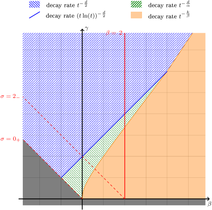
Figure 1: As $t\to+\infty$, decay rates are at most $O(t^{-k/\beta})$ if $-\beta<0<k<\gamma$ sufficiently close to $\gamma$ and $\gamma<\gamma_{\star}(\beta)$, with $\gamma_{\star}$ given by (11), and otherwise either $O(t^{-d/\alpha})$ if $\max\{0,-\beta\}<\gamma<2+\beta$ or $O(t^{-d/2})$ if $\gamma>\max\{2+\beta,-\beta\}$. The picture corresponds to $d=3$. In Case $\mathsf{L}=\mathsf{L}_{3}$, $\gamma$ is limited to the strip enclosed between the two dashed red lines.

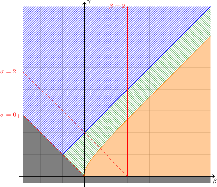
Figure 2: Decay rates depending on $\beta$ and $\gamma$ in dimension $d=2$, as $t\to+\infty$. The caption convention is the same as for Figure 1. When $\beta\geq 0$, the upper threshold of the region with decay rate $O(t^{-k/\beta})$, with $k$ close enough to $\gamma$, is $\gamma=\gamma_{\star}(\beta)$.

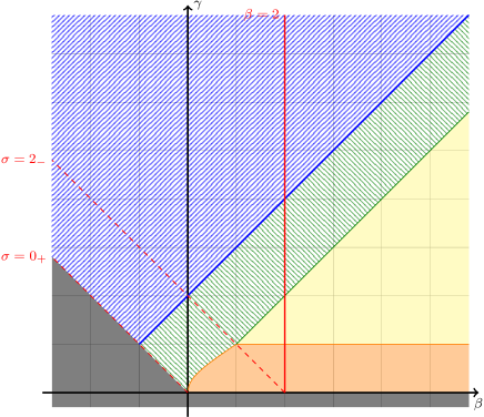
Figure 3: Decay rates depending on $\beta$ and $\gamma$ in dimension $d=1$, as $t\to+\infty$. When $\beta\geq 0$, $k$ is chosen arbitrarily close to $\gamma$. The caption convention is the same as for Figure 1 except for $1<\gamma<\beta$ which corresponds to the intermediate decay rate $\tau<\frac{2\gamma}{\gamma\left(\alpha-1\right)+\beta\left(\alpha+1\right)}$ indicated in Theorem 1.1.

The large time decay rates are governed by the scaling properties of (1). According to mellet_fractional_2011 ; MR2588245 (more references will be given later), a local equilibrium with fat tail implies that the diffusion limit involves a fractional diffusion operator. As in bouin_hypocoercivity_2017 , the key idea is that the (fractional) diffusion limit determines the rate of decay. Let us explain how the exponent $\alpha$ arises through a formal analysis in the case of the simple scattering operator $\mathsf{L}=\mathsf{L}_{2}$ corresponding to

$$\mathrm{b}(v,v^{\prime})=Z^{-1}\left\langle v\right\rangle^{-\beta}\left\langle v^{\prime}\right\rangle^{-\beta}\,,\quad Z:=\int_{{\mathbb{R}}^{d}}{\left\langle v\right\rangle^{-\beta}F(v)}\,\mathrm{d}v\,,\quad\beta\in{\mathbb{R}}\,.$$

Let us investigate the diffusion limit as $\varepsilon\to 0^{+}$ of the scaled kinetic equation written in terms of the Fourier variable $\xi$ corresponding to the macroscopic position variable $\varepsilon\,x$ :

$$\varepsilon^{\alpha}\,\partial_{t}\widehat{f}+i\,\varepsilon\,v\cdot\xi\,\widehat{f}=\mathsf{L}\widehat{f}\,.$$ (12)

The exponent $\alpha$, which determines the macroscopic time scale, is to be chosen. By the local mass conservation property, $\int_{{\mathbb{R}}^{d}}{\mathsf{L}f}\,\mathrm{d}v=0$, the spatial density, defined as

$$\rho_{f}(t,x):=\int_{{\mathbb{R}}^{d}}{f(t,x,v)}\,\mathrm{d}v\,,$$ (13)

solves in Fourier variables the continuity equation

$$\partial_{t}\widehat{\rho}_{f}+i\,\varepsilon^{1-\alpha}\int_{{\mathbb{R}}^{d}}{v\cdot\xi\,\widehat{f}}\,\mathrm{d}v=0\,.$$ (14)

The fractional diffusion limit $\varepsilon\to 0^{+}$ can be obtained by a formal Hilbert expansion as in Puel_2011 , in which only the case $\beta=0$ is covered, or as in MR3535408 , where the collision frequency is $|v|^{-\beta}$. Here we use a more direct computation.

Rewriting the scattering operator as

$$\mathsf{L}\widehat{f}=\left\langle v\right\rangle^{-\beta}\left(\mathsf{r}_{f}\,\frac{F}{Z}-\widehat{f}\right)\quad\mbox{with}\quad\mathsf{r}_{f}(t,\xi):=\int_{{\mathbb{R}}^{d}}{\left\langle v^{\prime}\right\rangle^{-\beta}\,\widehat{f}(t,\xi,v^{\prime})}\,\mathrm{d}v^{\prime}\,,$$

the kinetic equation (12) takes the form

$$\left(\left\langle v\right\rangle^{-\beta}+i\,\varepsilon\,v\cdot\xi\right)\widehat{f}=\left\langle v\right\rangle^{-\beta}\,\mathsf{r}_{f}\,\frac{F}{Z}-\varepsilon^{\alpha}\,\partial_{t}\widehat{f}\,.$$

The flux term in the continuity equation (14) can be rewritten as

$$i\,\varepsilon^{1-\alpha}\int_{{\mathbb{R}}^{d}}{v\cdot\xi\,\widehat{f}}\,\mathrm{d}v=\mathsf{b}_{\varepsilon}\frac{\mathsf{r}_{f}}{Z}-i\,\varepsilon\int_{{\mathbb{R}}^{d}}{\frac{v\cdot\xi\,\partial_{t}\widehat{f}}{\left\langle v\right\rangle^{-\beta}+i\,\varepsilon\,v\cdot\xi}}\,\mathrm{d}v\,,$$ (15)

with

$$\mathsf{b}_{\varepsilon}:=i\,\varepsilon^{1-\alpha}\int_{{\mathbb{R}}^{d}}{\frac{\left\langle v\right\rangle^{-\beta}\,v\cdot\xi\,F}{\left\langle v\right\rangle^{-\beta}+i\,\varepsilon\,v\cdot\xi}}\,\mathrm{d}v=\varepsilon^{2-\alpha}\int_{{\mathbb{R}}^{d}}{\frac{\left\langle v\right\rangle^{-\beta}\,(v\cdot\xi)^{2}\,F}{\left\langle v\right\rangle^{-2\,\beta}+\varepsilon^{2}\,(v\cdot\xi)^{2}}}\,\mathrm{d}v\,.$$ (16)

The second representation is due to the evenness of $F$. Recalling (2), we observe that the formal limit of the integral is finite for $\gamma>2+\beta$ and, by rotational symmetry, of the form $\kappa\,|\xi|^{2}$, for some $\kappa>0$. In this case the appropriate macroscopic time scale is diffusive, i.e., $\alpha=2$, and the macroscopic limit is the heat equation for the limiting spatial density $\rho_{0}$, written in Fourier variables,

$$\partial_{t}\widehat{\rho}_{0}+\kappa\,|\xi|^{2}\,\widehat{\rho}_{0}=0\,.$$

Here we use that formally $\lim_{\varepsilon\to 0}f=\rho_{0}\,F$, and therefore $\lim_{\varepsilon\to 0}\mathsf{r}_{f}=Z\,\widehat{\rho}_{0}$, and assume that the last term in (15) is a perturbation, which tends to zero.

Now let us consider the case $\gamma<2+\beta$. The computation of the asymptotic behaviour of $\mathsf{b}_{\varepsilon}$ is a bit tedious in this case. First note that in this case $\mathsf{b}_{\varepsilon}<\infty$ requires $\min\{1,\gamma\}+\beta>0$, which we assume in the following. With the coordinate change $v=(\varepsilon\,|\xi|)^{-1/(1+\beta)}\,w$, we obtain

$$\mathsf{b}_{\varepsilon}\approx\varepsilon^{\frac{\gamma+\beta}{1+\beta}-\alpha}\,|\xi|^{\frac{\gamma+\beta}{1+\beta}}\,\kappa\,,\quad\kappa:=c_{\gamma}\int_{{\mathbb{R}}^{d}}\frac{|w|^{-\beta-\gamma-d}\,(w\cdot\mathsf{e})^{2}}{|w|^{-2\,\beta}+(w\cdot\mathsf{e})^{2}}\,\mathrm{d}w$$

as $\varepsilon\to 0^{+}$, with $\mathsf{e}=\xi/|\xi|$. By rotational symmetry, $\kappa$ is independent from $\mathsf{e}\in\mathbb{S}^{d-1}$. The appropriate choice of the macroscopic time scale is now such that $\mathsf{b}_{\varepsilon}$ has a finite positive limit, which determines $\alpha$ as in (10). Our assumptions on $\beta$ and $\gamma$ imply $0<\alpha<2$. The macroscopic limit is the fractional heat equation

$$\partial_{t}\widehat{\rho}_{0}+\kappa\,|\xi|^{\alpha}\,\widehat{\rho}_{0}=0\,.$$ (17)

In the general case, $\alpha\leq 2$ covers the two cases, $\gamma\geq 2+\beta$ and $\gamma<2+\beta$, with a standard macroscopic limit when $\alpha=2$, and a fractional diffusion limit when $\alpha<2$. If $\rho$ solves (17), then

$$\frac{d}{dt}\|{\,\widehat{\rho}\,}\|_{\mathrm{L}^{2}(\mathrm{d}x)}^{2}=-\,2\,\kappa\,\|{\,|\xi|^{\frac{\alpha}{2}}\,\widehat{\rho}\,}\|_{\mathrm{L}^{2}(\mathrm{d}\xi)}^{2}\,.$$

Using the fractional Nash inequality

$$\|{\rho}\|_{\mathrm{L}^{2}(\mathrm{d}x)}\leq\mathcal{C}_{\mbox{Nash}}\,\|{\rho}\|_{\mathrm{L}^{1}(\mathrm{d}x)}^{\frac{\alpha}{d+\alpha}}\,\|{\,|\xi|^{\frac{\alpha}{2}}\,\widehat{\rho}\,}\|_{\mathrm{L}^{2}(\mathrm{d}\xi)}^{\frac{d}{d+\alpha}}\,,$$ (18)

and Plancherel’s identity, we obtain $\|{\rho(t,\cdot)}\|_{\mathrm{L}^{2}(\mathrm{d}x)}=O\big{(}t^{-d/\alpha}\big{)}$ as $t\to+\infty$. The proof of (18) can be found in Nash58 if $\alpha=2$ and the extension to the case $\alpha<2$ is straightforward. This heuristic analysis is responsible for the rates $\tau=d/\alpha$ of the solution of (1), at least under appropriate $\left\langle v\right\rangle\!{}^{k}$ moment conditions. At formal level, the decay estimates of the solution of (12) are uniform as $\varepsilon\to 0$. See Section 6.3 for additional comments.

For $\mathsf{L}=\mathsf{L}_{1}$ and $\mathsf{L}=\mathsf{L}_{3}$, we want to keep the same value for $\alpha$ as for $\mathsf{L}=\mathsf{L}_{2}$. This implicitly defines $\beta$. Technically, what matters is the Lyapunov function property, namely the fact that there exist three positive constant $a$, $b$ and $R$, a real parameter $\beta$, and a (smooth) positive Lyapunov function $F=F(v)$ on ${\mathbb{R}}^{d}$ such that

$$-\mathsf{L}F\leq\left(a\,\mathbbm{1}_{B_{R}}-b\left\langle v\right\rangle^{-\beta}\right)F$$

where $\mathsf{L}$ is a self-adjoint operator associated with a Dirichlet integral on the space of square integrable functions on ${\mathbb{R}}^{d}$ with respect to some probability measure. Details can be found for instance in bakry_rate_2008 . In integral form, this Lyapunov function property is used in Lemma 3, responsible for the interpolation inequality of Proposition 2, and finally for the decay rates of Theorems 1.1 and 1.2.

The expression of $\alpha$ can also be related with the macroscopic diffusion limit for $\mathsf{L}=\mathsf{L}_{1}$ and $\mathsf{L}=\mathsf{L}_{3}$. This is not as simple as for $\mathsf{L}=\mathsf{L}_{2}$ and we shall omit this computation here, even at formal level. The interested reader is invited to refer to bouin2020quantitative for such a justification.

Let us conclude this introduction by a brief review of the literature. Fractional diffusion limits of kinetic equations attracted a considerable interest in the recent years. The microscopic jump processes are indeed easy to encode in kinetic equations and the diffusion limit provides a simple procedure to justify the use of fractional operators at macroscopic level. Formal derivations are known for a long time, see for instance SCALAS_2003 , but rigorous proofs are more recent. In the case of linear scattering operators like those of Case $\mathsf{L}=\mathsf{L}_{2}$, we refer to mellet_fractional_2011 ; mellet_fractional_2010 ; Puel_2011 ; ben_abdallah_anomalous_2011 for some early results and to MR2588245 for a closely related work on Markov chains. Numerical schemes which are asymptotically preserving have been obtained in MR3470742 ; MR3535408 . Beyond the classical paper degond_diffusion_2000 , we also refer to mellet_fractional_2011 ; mellet_fractional_2010 ; Puel_2011 ; ben_abdallah_anomalous_2011 for a discussion of earlier results on standard, i.e., non-fractional, diffusion limits. Concerning the generalized Fokker-Planck operators of Case $\mathsf{L}=\mathsf{L}_{1}$, such that local equilibria have fat tails, the problem has recently been studied in MR3922536 in dimension $d=1$ by spectral methods and, from a probabilistic point of view, in fournier_one_2018 . Depending on the range of the exponents, various regimes corresponding to Brownian processes, stable processes or integrated symmetric Bessel processes are obtained and described in fournier_one_2018 as well as the threshold cases (some were already known, see for instance cattiaux2019diffusion ). Higher dimensional results have recently been obtained in fournier2018anomalous . Concerning Case $\mathsf{L}=\mathsf{L}_{3}$, the fractional diffusion limit of the fractional Vlasov-Fokker-Planck equation, or Vlasov–Lévy–Fokker–Planck equation, has been studied in cesbron_anomalous_2012 ; Aceves_Sanchez_2019 ; 2019arXiv191111535A when the friction force is proportional to the velocity. Here our Case $\mathsf{L}=\mathsf{L}_{3}$ is slightly different, as we pick forces giving rise to collision frequencies of the order of $|v|^{-\beta}$ as $|v|\to+\infty$. We refer to bouin2020quantitative for new results, a recent overview and further references.

In the homogeneous case, that is, when there is no $x$-dependence, it is classical to introduce a function $\Phi(v)=-\log F(v)$, where $F$ denotes the local equilibrium but is not necessarily of the form (2), and classify the possible behaviors of the solution $f$ to (1) according to the growth rate of $\Phi$. Assume that the collision operator is either the generalized Fokker-Planck operator of Case $\mathsf{L}=\mathsf{L}_{1}$ or the scattering operator of Case $\mathsf{L}=\mathsf{L}_{2}$. Schematically, if

$$\Phi(v)=\left\langle v\right\rangle^{\zeta}\,,$$

we obtain that $\|{f(t,\cdot)-M\,F}\|_{\mathrm{L}^{2}(\mathrm{d}\mu)}$ decays exponentially if $\zeta\geq 1$, with $M=\int_{{\mathbb{R}}^{d}}{f}\,\mathrm{d}v$. In the range $\zeta\in(0,1)$, the Poincaré inequality of Case $\mathsf{L}=\mathsf{L}_{1}$ has to be replaced by a weak Poincaré or a weighted Poincaré inequality: see rockner_weak_2001 ; kavian_fokker-planck_2015 ; BDLS and rates of convergence are typically algebraic in $t$. Summarizing, the lowest is the rate of growth of $\Phi$ as $|v|\to+\infty$, the slowest is the rate of convergence of $f$ to $M\,F$. Now let us focus on the limiting case as $\zeta\to 0^{+}$. The turning point precisely occurs for the minimal growth which guarantees that $F$ is integrable, at least for solutions of the homogeneous equation with initial data in $\mathrm{L}^{1}(\mathrm{d}v)$. Hence, if we consider

$$\Phi(v)=\eta\,\log\left\langle v\right\rangle,$$

with $\eta<d$, then diffusive effects win over confinement and the unique local equilibrium with finite mass is $0$. To measure the sharp rate of decay of $f$ towards $0$, one can replace the Poincaré inequality and the weak Poincaré or the weighted Poincaré inequalities by weighted Nash inequalities. See bouin_diffusion_2019 for details. In this paper, we consider the case $\eta=d+\gamma>d$, which guarantees that $F$ is integrable. Standard diffusion limits can be invoked if $\gamma>2+\beta$, but here we are also interested in the regime corresponding to fractional diffusion limits, with $\gamma\leq 2+\beta$.

As explained in Section 1, standard diffusion limits provide an interesting insight into the micro/macro decomposition which is the key of the $\mathrm{L}^{2}$-hypocoercive approach of dolbeault_hypocoercivity_2015 . Another parameter can be taken into account: the confinement in the spatial variable $x$. In presence of a confining potential $V=V(x)$ with sufficient growth and when $F$ has fast decay, typically for $\zeta\geq 1$, the rate of convergence is found to be exponential. A milder growth of $V$ gives a slower convergence rate as analyzed in cao_kinetic_2018 . If $e^{-V}$ is not integrable, the diffusion wins in the hypocoercive picture, and the rate of convergence of a finite mass solution of (1) towards $0$ can be captured by Nash and related Caffarelli-Kohn-Nirenberg inequalities: see bouin_hypocoercivity_2017 ; bouin_diffusion_2019 .

A typical regime for fractional diffusion limits is given by local equilibria with fat tails which behave according to (2) with $\gamma\in(0,2+\beta)$: $F$ is integrable but has no standard diffusion limit. Whenever fractional diffusion limits can be obtained, it was expected that rates of convergence can also be obtained by an adapted $\mathrm{L}^{2}$-hypocoercive approach. In this paper, we shall consider only the case $V=0$ and measure the decay rate. In view of lafleche_fractional_2020 (also see references therein), it is natural to expect that a fractional Nash type approach has to play the central role, and this is indeed what happens. The mode-by-mode hypocoercivity estimate shows that rates are of the order of $|\xi|^{\alpha}$ as $\xi\to 0$ which results in the expected time decay. In this direction, let us mention that the spectral information associated with $|\xi|^{\alpha}$ is very natural in connection with the fractional heat equation as was recently observed in ben-artzi_weak_2018 . As far as we know, asymptotic rates for (1) have not been studied so far, to the exception of the very recent results of 2019arXiv191111535A which deal with the Vlasov–Lévy–Fokker–Planck equation in the case of a spatial variable in the flat torus $\mathbb{T}^{d}$ by an $\mathrm{H}^{1}$-hypocoercivity method and the simplest version ($\beta=0$) of the scattering collision operator: see Section 6.2 for more details. A preliminary version of the present paper can be found in LaflechePhD2019 .

2 Outline of the method

2.1 Decay rates of the homogeneous solution

If $f$ is an homogeneous solution of (1), that is, a function independent from $x\in{\mathbb{R}}^{d}$, with initial datum $f^{\mathrm{in}}\in\mathrm{L}^{1}_{+}(\mathrm{d}v)\cap\mathrm{L}^{2}(\mathrm{d}\mu)$ such that $\int_{{\mathbb{R}}^{d}}{f^{\mathrm{in}}}\,\mathrm{d}v=1$, then

$$\frac{\mathrm{d}}{\mathrm{d}t}\,\|f-F\|^{2}=2\left\langle f,\mathsf{L}f\right\rangle\,.$$

It is natural to ask whether such an estimate proves the convergence of the solution $f(t,\cdot)$ to $F$ as $t\to+\infty$ and provides a rate of convergence. Let us assume that $\mathsf{L}$ is a self-adjoint operator on $\mathrm{L}^{2}(\mathrm{d}\mu)$ such that, for some $k\in(0,\gamma)$,
(i) the interpolation inequality

$$\int_{{\mathbb{R}}^{d}}{|g|^{2}}\,\mathrm{d}\mu\leq\mathcal{C}\,\Big{(}-\left\langle g,\mathsf{L}g\right\rangle\Big{)}^{\frac{1}{1+a}}\left(\int_{{\mathbb{R}}^{d}}{|g|^{2}\left\langle v\right\rangle^{k}}\,\mathrm{d}\mu\right)^{\frac{a}{1+a}}$$ (19)

holds for some $a>0$ and $\mathcal{C}>0$, if $\int_{{\mathbb{R}}^{d}}{g}\,\mathrm{d}\mu=0$,
(ii) there is a constant $\mathcal{C}_{k}$ such that

$$\forall\,t\geq 0\,,\quad\int_{{\mathbb{R}}^{d}}{|f(t,\cdot)|^{2}\left\langle v\right\rangle^{k}}\,\mathrm{d}\mu\leq\mathcal{C}_{k}\int_{{\mathbb{R}}^{d}}{\left|f^{\mathrm{in}}\right|^{2}\left\langle v\right\rangle^{k}}\,\mathrm{d}\mu\,.$$

Then  an elementary computation shows the algebraic decay rate

$$\forall\,t\geq 0\,,\quad\|f(t,\cdot)-F\|^{2}\leq\left(\|f^{\mathrm{in}}-F\|^{-2\,a}+\kappa\,a\,t\right)^{-1/a}$$

with $\kappa=2\,\mathcal{C}^{-(1+a)}\,\big{(}\mathcal{C}_{k}\int_{{\mathbb{R}}^{d}}{|f^{\mathrm{in}}|^{2}\left\langle v\right\rangle^{k}}\,\mathrm{d}\mu\big{)}^{-a}$. Note that the exponent $a$ depends on $k$. This result is an indication that also in the general spatially non-homogeneous case of (1), we cannot expect a better rate of convergence. The main difficulty there is to understand the interplay of the transport operator $v\cdot\nabla_{x}$ and of the collision operator $\mathsf{L}$, which is the main issue of this paper.

2.2 Non-homogeneous solutions: mode-by-mode analysis

Let us consider the measure $\mathrm{d}\mu=F^{-1}(v)\,\mathrm{d}v$ and the Fourier transform of $f$ in $x$ defined by

$$\widehat{f}(t,\xi,v):=\frac{1}{(2\pi)^{d/2}}\int_{{\mathbb{R}}^{d}}e^{-\,i\,x\cdot\xi}f(t,x,v)\,\mathrm{d}x\,.$$

If $f$ solves (1), then the equation satisfied by $\widehat{f}$ is

$$\partial_{t}\widehat{f}+\mathsf{T}\widehat{f}=\mathsf{L}\widehat{f}\,,\quad\widehat{f}(0,\xi,v)=\widehat{f}^{\mathrm{in}}(\xi,v)$$

where $\mathsf{T}$ is the transport operator in Fourier variables given by

$$\mathsf{T}\widehat{f}=i\,v\cdot\xi\,\widehat{f}\,,$$

and $\xi\in{\mathbb{R}}^{d}$ can be seen as a parameter, so that for each Fourier mode $\xi$, $\mathsf{T}$ is a multiplication operator and we can study the decay of $t\mapsto\widehat{f}(t,\xi,\cdot)$. For this reason, we call it a mode-by-mode analysis, as in bouin_hypocoercivity_2017 .

For any given $\xi\in{\mathbb{R}}^{d}$, taken as a parameter, we consider $(t,v)\mapsto\widehat{f}(t,\xi,v)$ on the complex valued Hilbert space $\mathrm{L}^{2}(\mathrm{d}\mu)$ with scalar product and norm given by (3). We define the orthogonal projection $\mathsf{\Pi}$ on the subspace generated by $F$ by

$$\mathsf{\Pi}\,f=\rho_{f}\,F\,,$$

where $\rho_{f}$ is given by (13) and observe that the property

$$\mathsf{\Pi}\mathsf{T}\mathsf{\Pi}=0$$

holds as a consequence of the radial symmetry of $F$. Let us define the operator

$$\mathsf{A}_{\xi}:=\frac{1}{\left\langle v\right\rangle^{2}}\,\mathsf{\Pi}\,\frac{\left(-\,i\,v\cdot\xi\right)\left\langle v\right\rangle^{\beta}}{1+\left\langle v\right\rangle^{2\,|1+\beta|}|\xi|^{2}}\,,$$

and the entropy functional by

$$\mathsf{H}_{\xi}[f]:=\|\widehat{f}\|^{2}+\delta\,\mathop{\mathrm{Re}}\left\langle\mathsf{A}_{\xi}\widehat{f},\widehat{f}\right\rangle\,.$$

The definition of $\mathsf{A}_{\xi}$ is reminiscent of the computation of $\mathsf{b}_{\varepsilon}$ in (16), with $\varepsilon=1$. In the case $\mathsf{L}=\mathsf{L}_{2}$ and $\beta\geq-1$, we can indeed notice that

$$\mathsf{A}_{\xi}\mathsf{T\,\Pi}=\frac{1}{\left\langle v\right\rangle^{2}}\,\mathsf{\Pi}\,\frac{\left(v\cdot\xi\right)^{2}\left\langle v\right\rangle^{\beta}}{1+\left\langle v\right\rangle^{2\,|1+\beta|}|\xi|^{2}}\,\mathsf{\Pi}=\frac{1}{\left\langle v\right\rangle^{2}}\,\mathsf{\Pi}\,\frac{\left\langle v\right\rangle^{-\beta}\left(v\cdot\xi\right)^{2}}{\left\langle v\right\rangle^{-2\,\beta}+\left\langle v\right\rangle^{2}|\xi|^{2}}\,\mathsf{\Pi}\,.$$

Compared with the expression $\mathsf{b}_{1}$, there are two minor differences: the $\left\langle v\right\rangle^{-2}$ factor is needed for technical reasons, in order to compute $\left\langle v\right\rangle$ moments and in particular $\mathsf{I}_{1}$ and $\mathsf{I}_{2}$ in Section 5.3; in the denominator of the symbol, $\left\langle v\right\rangle^{-2\,\beta}+(v\cdot\xi)^{2}$ is replaced by $\left\langle v\right\rangle^{-2\,\beta}+\left\langle v\right\rangle^{2}|\xi|^{2}$ which has similar scaling properties as $|v|\to+\infty$ but offers simpler integration properties. Moreover, the same definition for $\mathsf{A}_{\xi}$ can be used in the cases $\mathsf{L}=\mathsf{L}_{1}$ and $\mathsf{L}=\mathsf{L}_{3}$. The first elementary result is the observation that $\mathsf{A}_{\xi}$ is a bounded operator and that $\mathsf{H}_{\xi}[f]$ is equivalent to $\|f\|^{2}$ if $\delta>0$ is not too large.

Lemma 1

With the above notation, for any $\delta\in(0,2)$ and $f\in\mathrm{L}^{2}(\mathrm{d}\mu)$, we have

$$|\left\langle\mathsf{A}_{\xi}f,f\right\rangle|\leq\frac{1}{2}\,\|f\|^{2}\quad\mbox{and}\quad\left(2-\delta\right)\|f\|^{2}\leq 2\,\mathsf{H}_{\xi}[f]\leq\left(2+\delta\right)\|f\|^{2}\,.$$

We shall use the notation

$$\varphi(\xi,v):=\frac{\left\langle v\right\rangle^{\beta}}{1+\left\langle v\right\rangle^{2\,|1+\beta|}|\xi|^{2}}\quad\mbox{and}\quad\psi(v):=\left\langle v\right\rangle^{-2},$$

and may notice that $\mathsf{A}_{\xi}\widehat{f}=\psi\,\mathsf{\Pi}\mathsf{T}^{*}\,\varphi\,\widehat{f}$, where $\mathsf{T}^{*}$ denotes the dual of $\mathsf{T}$ acting on $\mathrm{L}^{2}(\mathrm{d}\mu)$.

Proof (Proof of Lemma 1)

With these definitions, we obtain $|\psi|\leq 1$ and $\left|(v\cdot\xi)\,\varphi(\xi,v)\right|\leq 1/2$, so that the Cauchy-Schwarz inequality yields

$$\left|\left\langle\mathsf{A}_{\xi}f,f\right\rangle\right|^{2}\leq\int_{{\mathbb{R}}^{d}}|\psi(v)|^{2}\,|f(\xi,v)|^{2}\,\mathrm{d}v\int_{{\mathbb{R}}^{d}}|(v\cdot\xi)\,\varphi(\xi,v)|^{2}\,|f(\xi,v)|^{2}\,\mathrm{d}v\leq\frac{1}{4}\,\|f\|^{4}\,,$$

which completes the proof of Lemma 1.  ∎

We observe that if $f$ solves (1), then

$$\frac{\mathrm{d}}{\mathrm{d}t}\mathsf{H}_{\xi}[\widehat{f}]=-\mathsf{D}_{\xi}[\widehat{f}]:=\,2\,\langle\mathsf{L}\widehat{f},\widehat{f}\rangle-\delta\,\mathsf{R}_{\xi}[\widehat{f}]$$

where $\mathsf{R}_{\xi}[\widehat{f}]=-\,\frac{\mathrm{d}}{\mathrm{d}t}\mathop{\mathrm{Re}}\,\langle\mathsf{A}_{\xi}\widehat{f},\widehat{f}\rangle$. Our goal is to relate $\mathsf{H}_{\xi}[\widehat{f}]$ and $\mathsf{D}_{\xi}[\widehat{f}]$. Any decay rate of $\mathsf{H}_{\xi}[\widehat{f}]$ obtained by a Grönwall estimate gives us a decay rate for $\|f\|^{2}$ by Lemma 1 and, using an inverse Fourier transform, in $\mathrm{L}^{2}(\mathrm{d}x\,\mathrm{d}\mu)$.

More notation will be needed. Let us define the weighted norms

$$\|{g}\|_{k}^{2}:=\int_{{\mathbb{R}}^{d}}|g|^{2}\left\langle v\right\rangle^{k}\mathrm{d}\mu\,,$$

so that in particular $\|g\|=\|{g}\|_{0}$. A crucial observation, which will be used repeatedly, is the fact that for any constant $\kappa>0$,

$$\|{g-\kappa\,F}\|_{k}^{2}=\|{g}\|_{k}^{2}+\kappa^{2}\int_{{\mathbb{R}}^{d}}\left\langle v\right\rangle^{k}F\,\mathrm{d}v-2\,\kappa\int_{{\mathbb{R}}^{d}}\left\langle v\right\rangle^{k}g\,\mathrm{d}v\geq\|{(1-\mathsf{\Pi}_{k})\,g}\|_{k}^{2}$$

where

$$\mathsf{\Pi}_{k}\,g:=\frac{\int_{{\mathbb{R}}^{d}}\left\langle v\right\rangle^{k}g\,\mathrm{d}v}{\int_{{\mathbb{R}}^{d}}\left\langle v\right\rangle^{k}F\,\mathrm{d}v}\,F\,.$$

This is easily shown by optimizing the left-hand side of the inequality on $\kappa\in{\mathbb{R}}$. Notice that $\mathsf{\Pi}_{0}=\mathsf{\Pi}$.

The parameters $\beta$ and $\gamma$ are chosen as in Theorems 1.1 and 1.2 while $\alpha$ is given by (10): $\alpha=\frac{\gamma+\beta}{1+\beta}$ if $\gamma<2+\beta$ and $\alpha=2$ if $\gamma\geq 2+\beta$. For simplicity, we shall not keep track of all constants and simply write that $\mathsf{a}\lesssim\mathsf{b}$ and $\mathsf{a}\gtrsim\mathsf{b}$ if there is a positive constant $\mathsf{c}$ such that, respectively, $\mathsf{a}\leq\mathsf{b}\,\mathsf{c}$ and $\mathsf{a}\geq\mathsf{b}\,\mathsf{c}$. We also define $\omega_{d}:=|\mathbb{S}^{d-1}|$ where $\mathbb{S}^{d-1}$ denotes the unit sphere in ${\mathbb{R}}^{d}$.

2.3 Outline of the method and key intermediate estimates

Assume that $f$ is a finite mass solution of (1) on ${\mathbb{R}}_{+}\times{\mathbb{R}}^{d}\times{\mathbb{R}}^{d}$. Our goal is to relate

$$\mathsf{H}[f]:=\int_{{\mathbb{R}}^{d}}\mathsf{H}_{\xi}[\widehat{f}]\,\mathrm{d}\xi$$

and

$$-\,\frac{\mathrm{d}}{\mathrm{d}t}\mathsf{H}[f]=-\,2\,\iint_{{\mathbb{R}}^{d}\times{\mathbb{R}}^{d}}{f\,\mathsf{L}f}\,\mathrm{d}x\,\mathrm{d}\mu+\delta\int_{{\mathbb{R}}^{d}}\mathsf{R}_{\xi}[\widehat{f}]\,\mathrm{d}\xi$$

by a differential inequality and use a Grönwall estimate. According to Lemma 1, the decay rate of $\|f\|^{2}$ is the same as for $\mathsf{H}_{\xi}[\widehat{f}]$. Under Assumption (H), we consider a solution $f$ of (1) with initial condition $f^{\mathrm{in}}\in\mathrm{L}^{1}(\mathrm{d}x\,\mathrm{d}v)\cap\mathrm{L}^{2}(\mathrm{d}x\,\mathrm{d}\mu)$. The main steps of our method are as follows:

$\rhd$ The solution is bounded in a weighted $\mathrm{L}^{2}$ space. We shall prove the following result in Section 3.

Proposition 1

Assume that (H) holds. Let $d\geq 1$, $\gamma>0$, $\gamma+\beta\geq 0$, $k\in(0,\gamma)$ and $f$ be a solution of (1) with initial condition $f^{\mathrm{in}}\in\mathrm{L}^{2}(\left\langle v\right\rangle^{k}\mathrm{d}x\,\mathrm{d}\mu)$. Then, there exists a positive constant $\mathcal{C}_{k}$ depending on $d$, $\gamma$, $\beta$ and $k$ such that

$$\forall\,t\geq 0\,,\quad\|{f(t,\cdot,\cdot)}\|_{\mathrm{L}^{2}(\left\langle v\right\rangle^{k}\mathrm{d}x\,\mathrm{d}\mu)}\leq\mathcal{C}_{k}\,\|{f^{\mathrm{in}}}\|_{\mathrm{L}^{2}(\left\langle v\right\rangle^{k}\mathrm{d}x\,\mathrm{d}\mu)}\,.$$

$\rhd$ The collision term controls the distance to the local equilibrium. We have the following microscopic coercivity estimate.

Proposition 2

Let $d\geq 1$, $\gamma>0$, $\gamma+\beta\geq 0$, $\eta\in[-\beta,\gamma)$ and $k\in(0,\gamma)$. Assume that $\beta=\,2$ if $\mathsf{L}=\mathsf{L}_{1}$, that Assumptions (5)–(8) hold if $\mathsf{L}=\mathsf{L}_{2}$, and that $\sigma\in(0,2)$, $\beta=\sigma-\gamma$ if $\mathsf{L}=\mathsf{L}_{3}$. Then there exists a positive constant $\mathcal{C}$ depending on $\|{f}\|_{\mathrm{L}^{2}(\mathrm{d}x\,\mathrm{d}\mu)}$ such that for any $f\in\mathrm{L}^{2}(\left\langle v\right\rangle^{k}\mathrm{d}x\,\mathrm{d}\mu)$,

$$\mathcal{C}\,\|{(1-\mathsf{\Pi}_{\eta})f}\|_{\mathrm{L}^{2}(\mathrm{d}x\,\left\langle v\right\rangle^{\eta}\mathrm{d}\mu)}^{2\,\frac{k+\beta}{k-\eta}}\,\|{f}\|_{\mathrm{L}^{2}(\mathrm{d}x\,\left\langle v\right\rangle^{k}\mathrm{d}\mu)}^{-\,2\,\frac{\eta+\beta}{k-\eta}}\leq-\iint_{{\mathbb{R}}^{d}\times{\mathbb{R}}^{d}}{f\,\mathsf{L}f}\,\mathrm{d}x\,\mathrm{d}\mu\,.$$

This estimate is the extension of (19) to the non-homogeneous case. The proof is done in Section 4. We shall use Proposition 2 with $\eta=-\beta$ if $\gamma>\beta$ and for some $\eta\in(-\,\gamma,0)$ if $\gamma\leq\beta$. The case $\eta\geq 0$ is needed only in Step 4 of the proof of Proposition 3.

$\rhd$ Our proofs require the computation of a large number of coefficients and various estimates which are collected in Sections 5.1 and 5.2.

$\rhd$ A microscopic coercivity estimate is established in Section 5.3, which goes as follows. Let us define the function

$$\mathcal{L}(\xi):=\frac{|\xi|^{\alpha}}{\left\langle\xi\right\rangle^{\alpha}}\quad\mbox{if}\quad\gamma\neq 2+\beta\,,\quad\mathcal{L}(\xi):=\frac{|\xi|^{2}\,\big{|}\log|\xi|\big{|}}{1+|\xi|^{2}\,\log|\xi|}\quad\mbox{if}\quad\gamma=2+\beta\,.$$

Proposition 3

Let $\gamma>\max\{0,-\beta\}$ and $\eta\in(-\,\gamma,\gamma)$ such that $\eta\geq-\beta$. Under Assumption (H), there exists a positive, bounded function $\xi\mapsto\mathcal{K}(\xi)$ such that

$$\mathsf{R}_{\xi}[\widehat{f}]\gtrsim\mathcal{L}(\xi)\,\|\mathsf{\Pi}\widehat{f}\|^{2}-\mathcal{K}(\xi)\,\|{(1-\mathsf{\Pi})\widehat{f}}\|_{\eta}^{2}\,.$$

In Section 5.4, inspired by fractional Nash inequalities, we deduce from Proposition 3 an estimate on the distance in the direction which is orthogonal to the local equilibria.

Corollary 1

Under Assumption (H), we have

$$\int_{{\mathbb{R}}^{d}}\mathsf{R}_{\xi}[\widehat{f}]\,\mathrm{d}\xi\;\gtrsim\;\|{\mathsf{\Pi}f}\|_{\mathrm{L}^{2}(\mathrm{d}x\,\mathrm{d}\mu)}^{2\,(1+\frac{\alpha}{d})}-{\left|\kern-1.07639pt\left|\kern-1.07639pt\left|(1-\mathsf{\Pi})f\right|\kern-1.07639pt\right|\kern-1.07639pt\right|}_{-\beta}^{2}\quad\mbox{if}\quad\gamma\neq 2+\beta\,,$$

$$\int_{{\mathbb{R}}^{d}}\mathsf{R}_{\xi}[\widehat{f}]\,\mathrm{d}\xi\;\gtrsim\;\|{\mathsf{\Pi}f}\|_{\mathrm{L}^{2}(\mathrm{d}x\,\mathrm{d}\mu)}^{2\,(1+\frac{\alpha}{d})}\,\log\left(\frac{\;\|{\mathsf{\Pi}f}\|_{\mathrm{L}^{2}(\mathrm{d}x\,\mathrm{d}\mu)}}{\;\|{f}\|_{\mathrm{L}^{1}(\mathrm{d}x\,\mathrm{d}\mu)}}\right)-{\left|\kern-1.07639pt\left|\kern-1.07639pt\left|(1-\mathsf{\Pi})f\right|\kern-1.07639pt\right|\kern-1.07639pt\right|}_{-\beta}^{2}\\ \mbox{if}\quad\gamma=2+\beta\,.$$

The proof is a straightforward consequence of Lemma 14 if $\gamma\neq 2+\beta$ and of Lemma 15 if $\gamma=2+\beta$. See details in Section 5.4 and 5.5.

2.4 Sketch of the proof of the main results

The difficult part of the paper is the proof of Propositions 1, 2 and 3, and Corollary 1. If $\gamma\leq\beta$, we have to take $\eta\neq-\beta$ and use additional interpolation estimates: see Section 6. Otherwise, the proof of Theorems 1.1 and 1.2 is not difficult if $\gamma>\beta$ and can be done as follows.

Under Assumption (H), a solution of (1) is such that

$$-\,\frac{\mathrm{d}}{\mathrm{d}t}\mathsf{H}[f]=-2\iint_{{\mathbb{R}}^{d}\times{\mathbb{R}}^{d}}{f\,\mathsf{L}f}\,\mathrm{d}x\,\mathrm{d}\mu-\delta\int_{{\mathbb{R}}^{d}}\mathsf{R}_{\xi}[\widehat{f}]\,\mathrm{d}\xi\,.$$

Let us assume that $\gamma\neq 2+\beta$ and $\gamma>\beta$. We rely on Proposition 2.
$\bullet$ If $\beta\leq 0$, with $\eta=-\beta$, we find that

$$\int_{{\mathbb{R}}^{d}}\mathsf{R}_{\xi}[\widehat{f}]\,\mathrm{d}\xi\gtrsim\|{\mathsf{\Pi}f}\|_{\mathrm{L}^{2}(\mathrm{d}x\,\mathrm{d}\mu)}^{2\,(1+\frac{\alpha}{d})}-{\left|\kern-1.07639pt\left|\kern-1.07639pt\left|(1-\mathsf{\Pi})f\right|\kern-1.07639pt\right|\kern-1.07639pt\right|}_{-\beta}^{2}\,.$$

We obtain

$$-\,\frac{\mathrm{d}}{\mathrm{d}t}\mathsf{H}[f] \gtrsim(1-\delta)\,{\left|\kern-1.07639pt\left|\kern-1.07639pt\left|(1-\mathsf{\Pi})f\right|\kern-1.07639pt\right|\kern-1.07639pt\right|}_{-\beta}^{2}+\delta\,\|{\mathsf{\Pi}f}\|_{\mathrm{L}^{2}(\mathrm{d}x\,\mathrm{d}\mu)}^{2\,(1+\frac{\alpha}{d})}$$

$$\gtrsim(1-\delta)\,\|{(1-\mathsf{\Pi})f}\|_{\mathrm{L}^{2}(\mathrm{d}x\,\mathrm{d}\mu)}^{2}+\delta\,\|{\mathsf{\Pi}f}\|_{\mathrm{L}^{2}(\mathrm{d}x\,\mathrm{d}\mu)}^{2\,(1+\frac{\alpha}{d})}$$

$$\gtrsim\mathsf{H}[f]^{2\,(1+\frac{\alpha}{d})}$$

using the simple observation that $\|{(1-\mathsf{\Pi})f}\|_{-\beta}^{2}\geq\|{(1-\mathsf{\Pi})f}\|_{\mathrm{L}^{2}(\mathrm{d}\mu)}^{2}$ if $\beta\leq 0$.
$\bullet$ If $\beta\in(0,\gamma)$ and $2+\beta\neq\gamma>\beta$, again with $\eta=-\beta$, we find that

$$-\,\frac{\mathrm{d}}{\mathrm{d}t}\mathsf{H}[f]\gtrsim(1-\delta){\left|\kern-1.07639pt\left|\kern-1.07639pt\left|(1-\mathsf{\Pi})f\right|\kern-1.07639pt\right|\kern-1.07639pt\right|}_{-\beta}^{2}+\delta\,\|{\mathsf{\Pi}f}\|_{\mathrm{L}^{2}(\mathrm{d}x\,\mathrm{d}\mu)}^{2\,(1+\frac{\alpha}{d})}\,.$$

Using Hölder’s inequality

$$\|(1-\mathsf{\Pi})f\|^{2}\leq\|{(1-\mathsf{\Pi})f}\|_{-\beta}^{\frac{2\,k}{k+\beta}}\,\|{(1-\mathsf{\Pi})f}\|_{k}^{\frac{\beta-2}{k+\beta}}\,,$$

we conclude that

$$-\,\frac{\mathrm{d}}{\mathrm{d}t}\mathsf{H}[f]\gtrsim(1-\delta)\|{(1-\mathsf{\Pi})f}\|_{\mathrm{L}^{2}(\mathrm{d}x\,\mathrm{d}\mu)}^{2\,(1+\frac{\beta}{k})}+\delta\,\|{\mathsf{\Pi}f}\|_{\mathrm{L}^{2}(\mathrm{d}x\,\mathrm{d}\mu)}^{2\,(1+\frac{\alpha}{d})}\,.$$

$\bullet$ If $d\geq 1$, $\beta\geq 0$ and $\gamma=2+\beta$, $\alpha=2$ but there is a logarithmic correction in the expression of $\int_{{\mathbb{R}}^{d}}\mathsf{R}_{\xi}[\widehat{f}]\,\mathrm{d}\xi$, which is responsible for the $O(\log t)$ correction of Theorems 1.1 and 1.2 in case $\gamma=2+\beta$ as $t\to+\infty$.
$\bullet$ For integrability reasons, the case $\gamma\leq\beta$ requires further estimates involving some $\eta\in(-\,\gamma,0)$ that will be dealt with in Sections 4.4 and 6.1. Except in this case, the proof of Theorems 1.1 and 1.2 is complete.

3 Estimates in weighted $\mathrm{L}^{2}$ spaces

In this section, we assume that $\beta\geq 0$.

3.1 A result in weighted $\mathrm{L}^{2}$ spaces

Let us prove Proposition 1, i.e., the propagation of weighted norms $\mathrm{L}^{2}(\left\langle v\right\rangle^{k}\mathrm{d}x\,\mathrm{d}\mu)$ with power law of order $k\in(0,\gamma)$.

The conservation of weighted norms has also been used in BDLS when $F$ has a sub-exponential form. In that case, any value of $k$ was authorized, and this was implicitly a consequence of the fact that such a local equilibrium $F$ had finite weighted norms $\mathrm{L}^{2}(\left\langle v\right\rangle^{k}\mathrm{d}x\,\mathrm{d}\mu)$ for any $k\in{\mathbb{R}}_{+}$. For a local equilibrium given by (2), there is a limitation on $k$ as we cannot expect a global propagation of higher moments than those of $F$.

For any function $h\in\mathrm{L}^{2}(\left\langle v\right\rangle^{k}\mathrm{d}x\,\mathrm{d}\mu)$, one can notice that

$$\|{h}\|_{\mathrm{L}^{2}(\left\langle v\right\rangle^{k}\mathrm{d}x\,\mathrm{d}\mu)}=\|{F^{-1}h}\|_{\mathrm{L}^{2}(F\left\langle v\right\rangle^{k}\mathrm{d}x\,\mathrm{d}v)}\,.$$

In other words, it is equivalent to control the semi-group $e^{(\mathsf{L}-\mathsf{T})t}$ in $\mathrm{L}^{2}(\left\langle v\right\rangle^{k}\mathrm{d}x\,\mathrm{d}\mu)$ and $F^{-1}\,e^{(\mathsf{L}-\mathsf{T})t}$ in $\mathrm{L}^{2}(F\left\langle v\right\rangle^{k}\mathrm{d}x\,\mathrm{d}v)$. Since $\mathrm{L}^{2}(\left\langle v\right\rangle^{k}F\,\mathrm{d}x\,\mathrm{d}v)$ is a space interpolating between $\mathrm{L}^{1}(F\left\langle v\right\rangle^{k}\mathrm{d}x\,\mathrm{d}v)$ and $\mathrm{L}^{\infty}(\mathrm{d}x\,\mathrm{d}v)$ (see (stein_interpolation_1958, , Theorem (2.9))), we shall establish the result of Proposition 1 by proving that $F^{-1}\,e^{(\mathsf{L}-\mathsf{T})t}$ is bounded onto $\mathrm{L}^{\infty}(\mathrm{d}x\,\mathrm{d}v)$ in Section 3.2 and onto $\mathrm{L}^{1}(F\left\langle v\right\rangle^{k}\mathrm{d}x\,\mathrm{d}v)$ in Section 3.5. In order to prove this last estimate, as in kavian_fokker-planck_2015 ; lafleche_fractional_2020 ; BDLS , we shall use a Lyapunov function method in Section 3.3 and a splitting of the operator in Section 3.4.

3.2 The boundedness in $\mathrm{L}^{\infty}(\mathrm{d}x\,\mathrm{d}v)$

Lemma 2

Let $d\geq 1$ and $\gamma>0$. If (H) holds, then

$$\forall\,t\geq 0\,,\quad\|{F^{-1}e^{t(\mathsf{L}-\mathsf{T})}}\|_{\mathrm{L}^{\infty}(\mathrm{d}x\,\mathrm{d}v)\to\mathrm{L}^{\infty}(\mathrm{d}x\,\mathrm{d}v)}\leq 1\,,$$

where the norm $\|{\cdot}\|_{X\to Y}$ denotes the operator norm for an operator with domain $X$ and codomain $Y$.

Proof

This is a consequence of the maximum principle in Case $\mathsf{L}=\mathsf{L}_{1}$. In Case $\mathsf{L}=\mathsf{L}_{2}$, $h^{\#}(t,x,v)=F^{-1}(v)\,f(t,x+v\,t,v)$ solves

$$\partial_{t}h^{\#}+\nu(v)\,h^{\#}=\int_{{\mathbb{R}}^{d}}\mathrm{b}(v,v^{\prime})\,F(v^{\prime})\,h^{\#}(t,x,v^{\prime})\,\mathrm{d}v^{\prime}\,,$$

which is clearly a positivity preserving equation. The positivity of

$$(t,x,v)\mapsto\|{h(0,\cdot,\cdot)}\|_{\mathrm{L}^{\infty}(\mathrm{d}x\,\mathrm{d}v)}-h^{\#}(t,x,v)$$

is also preserved, as it solves the same equation, which proves the claim. Case $\mathsf{L}=\mathsf{L}_{3}$ is less standard as it relies on the maximum principle for fractional operators. As this is out of the scope of the present paper, we will only sketch the main steps of a proof. First of all, the results of lafleche_fractional_2020 can be adapted to $E$ as defined by (9), thus proving that the evolution according to $\partial_{t}-F\,\mathsf{L}_{3}(F^{-1}\cdot)$ preserves $\mathrm{L}^{\infty}$ bounds. This is also the case of $\partial_{t}-\mathsf{T}$. We can then conclude using a time-splitting approximation scheme of evolution and a Trotter formula.  ∎

3.3 A Lyapunov function method

The boundedness of the operator $F^{-1}e^{t(\mathsf{L}-\mathsf{T})}$ in $\mathrm{L}^{1}(F\left\langle v\right\rangle^{k}\mathrm{d}x\,\mathrm{d}v)$ is equivalent to the boundedness of the operator $e^{t(\mathsf{L}-\mathsf{T})}$ in $\mathrm{L}^{1}(\left\langle v\right\rangle^{k}\mathrm{d}x\,\mathrm{d}v)$. To obtain such a bound, we rely on a Lyapunov function estimate.

Lemma 3

Let $d\geq 1$, $\beta\geq 0$ and $\gamma>0$. If (H) holds, then for any $k\in[0,\gamma+\beta)$, there exists $(a,b,R)\in{\mathbb{R}}\times{\mathbb{R}}_{+}\times{\mathbb{R}}_{+}$ such that for any $f\in\mathrm{L}^{1}(\left\langle v\right\rangle^{k}\mathrm{d}x\,\mathrm{d}v)$,

$$\iint_{{\mathbb{R}}^{d}\times{\mathbb{R}}^{d}}\tfrac{f}{|f|}\,\mathsf{L}f\,\left\langle v\right\rangle^{k}\mathrm{d}x\,\mathrm{d}v\leq\iint_{{\mathbb{R}}^{d}\times{\mathbb{R}}^{d}}\left(a\,\mathds{1}_{B_{R}}-b\left\langle v\right\rangle^{-\beta}\right)|f|\left\langle v\right\rangle^{k}\mathrm{d}x\,\mathrm{d}v\,.$$

As a special case corresponding to $k=0$, we have $\iint_{{\mathbb{R}}^{d}\times{\mathbb{R}}^{d}}\tfrac{f}{|f|}\,\mathsf{L}f\,\mathrm{d}x\,\mathrm{d}v\leq 0$.

Here by convention, we shall write that $\tfrac{f}{|f|}=0$ if $f=0$.

Proof

First assume that $f\geq 0$. Then one may write,

$$\iint_{{\mathbb{R}}^{d}\times{\mathbb{R}}^{d}}\mathsf{L}f\,\left\langle v\right\rangle^{k}\mathrm{d}x\,\mathrm{d}v=\iint_{{\mathbb{R}}^{d}\times{\mathbb{R}}^{d}}\mathsf{L}f\,F\left\langle v\right\rangle^{k}\mathrm{d}x\,\mathrm{d}\mu\\ =\iint_{{\mathbb{R}}^{d}\times{\mathbb{R}}^{d}}\mathsf{L}^{*}(F\left\langle v\right\rangle^{k})\,f\,\mathrm{d}x\,\mathrm{d}\mu\,.$$

$\bullet$ In Case $\mathsf{L}=\mathsf{L}_{1}$, we notice that $\mathsf{L}$ is self-adjoint on $\mathrm{L}^{2}(\mathrm{d}\mu)$, recall that $\beta=2$ and compute

$$F^{-1}\,\mathsf{L}_{1}\big{(}F\left\langle\cdot\right\rangle^{k}\big{)}(v) =\left\langle v\right\rangle^{d+\gamma}\nabla_{v}\cdot\left(\left\langle v\right\rangle^{-d-\gamma}\nabla_{v}\left\langle v\right\rangle^{k}\right)$$

$$=k\left\langle v\right\rangle^{d+\gamma}\,\nabla_{v}\cdot\left(\left\langle v\right\rangle^{-d-\gamma+k-2}v\right)$$

$$=k\left(d+\gamma-k+2\right)\left\langle v\right\rangle^{k-4}-k\left(\gamma+2-k\right)\left\langle v\right\rangle^{k-2}$$

and obtain the result for any $k<\gamma+\beta=\gamma+2$.

$\bullet$ In Case $\mathsf{L}=\mathsf{L}_{2}$, by Assumption (5) one obtains that

$$F^{-1}\,\mathsf{L}_{2}^{*}\big{(}F\left\langle\cdot\right\rangle^{k}\big{)}(v) =\int_{{\mathbb{R}}^{d}}\mathrm{b}(v^{\prime},v)\left(\left\langle v^{\prime}\right\rangle^{k}F(v^{\prime})-\left\langle v\right\rangle^{k}F(v^{\prime})\right)\mathrm{d}v^{\prime}$$

$$=\left(\int_{{\mathbb{R}}^{d}}\mathrm{b}(v^{\prime},v)\frac{\left\langle v^{\prime}\right\rangle^{k}}{\left\langle v\right\rangle^{k}}\,F(v^{\prime})\,\mathrm{d}v^{\prime}-\nu(v)\right)\left\langle v\right\rangle^{k}\,.$$

By Assumption (7), $\mathcal{C}_{\mathrm{b}}(k)=\sup_{v\in{\mathbb{R}}^{d}}\left\langle v\right\rangle^{\beta}\int_{{\mathbb{R}}^{d}}\mathrm{b}(v^{\prime},v)\left\langle v^{\prime}\right\rangle^{k}F(v^{\prime})\,\mathrm{d}v^{\prime}$ is finite for any $k\in(0,\gamma+\beta)$, and as a consequence, we know that

$$\quad\forall\,v\in{\mathbb{R}}^{d}\,,\quad\nu(v)\leq\int_{{\mathbb{R}}^{d}}\mathrm{b}(v^{\prime},v)\left\langle v^{\prime}\right\rangle^{k}F(v^{\prime})\,\mathrm{d}v^{\prime}\leq\mathcal{C}_{\mathrm{b}}(k)\left\langle v\right\rangle^{-\beta}.$$

This yields

$$F^{-1}\,\mathsf{L}_{2}^{*}\big{(}F\,\left\langle\cdot\right\rangle^{k}\big{)}(v)\leq\left(\frac{\mathcal{C}_{\mathrm{b}}(b)}{\left\langle v\right\rangle^{k}}-\frac{\nu(v)}{\left\langle v\right\rangle^{-\beta}}\right)\left\langle v\right\rangle^{-\beta}\,.$$

We conclude that Inequality (3) holds for any $k\in(0,\gamma+\beta)$ by Assumption (4).

$\bullet$ In Case $\mathsf{L}=\mathsf{L}_{3}$, it is elementary to compute $\mathsf{L}_{3}^{*}$ and observe that

$$F^{-1}\,\mathsf{L}_{3}^{*}\big{(}F\,\left\langle\cdot\right\rangle^{k}\big{)}(v) =\Delta_{v}^{\sigma/2}\left\langle v\right\rangle^{k}-E(v)\,\cdot\nabla_{v}\left\langle v\right\rangle^{k}$$

$$=\left[\left\langle v\right\rangle^{-k}\Delta_{v}^{\sigma/2}\left\langle v\right\rangle^{k}-k\left(v\cdot E\right)\left\langle v\right\rangle^{-2}\right]\left\langle v\right\rangle^{k},$$

$$\leq\left[\left\langle v\right\rangle^{-k}\Delta_{v}^{\sigma/2}\left\langle v\right\rangle^{k}-C\,\left\langle v\right\rangle^{-\beta}\right]\left\langle v\right\rangle^{k},$$

where the estimate $k\left(v\cdot E\right)\left\langle v\right\rangle^{-2}\geq C\,\left\langle v\right\rangle^{-\beta}$ for some $C>0$ arises as a consequence of Proposition 7. According to (biler_blowup_2009, , Lemma 3.1) (also see biler_blowup_2010 ; lafleche_fractional_2020 ), we have

$$\forall\,v\in{\mathbb{R}}^{d}\,,\quad\Delta_{v}^{\sigma/2}\left\langle v\right\rangle^{k}\lesssim\left\langle v\right\rangle^{k-\sigma}\,,$$

under the condition that $k<\sigma=\gamma+\beta$. This again completes the proof of Inequality (3).

When $f$ changes sign, it is possible to reduce the problem to the case $f\geq 0$ as follows. In Case $\mathsf{L}=\mathsf{L}_{1}$, we use Kato’s inequality to assert that

$$\frac{f}{|f|}\,\Delta_{v}f\leq\Delta_{v}|f|$$

in the sense of Radon measures (see (MR333833, , Lemma A) or, for instance, (brezis_katos_2004, , Theorem 1.1)). Case $\mathsf{L}=\mathsf{L}_{2}$ relies on the elementary observation that

$$\iint_{{\mathbb{R}}^{d}\times{\mathbb{R}}^{d}}\tfrac{f}{|f|}\,\mathsf{L}_{2}f\left\langle v\right\rangle^{k}\mathrm{d}v\,\mathrm{d}v^{\prime} =\iint_{{\mathbb{R}}^{d}\times{\mathbb{R}}^{d}}\mathrm{b}(v,v^{\prime})\,f^{\prime}\,\frac{f}{|f|}\,F\left\langle v\right\rangle^{k}\mathrm{d}v\,\mathrm{d}v^{\prime}-\int_{{\mathbb{R}}^{d}}\nu\,|f|\,\mathrm{d}v$$

$$\leq\iint_{{\mathbb{R}}^{d}\times{\mathbb{R}}^{d}}\mathrm{b}(v,v^{\prime})\,|f^{\prime}|\,F\left\langle v\right\rangle^{k}\mathrm{d}v\,\mathrm{d}v^{\prime}-\int_{{\mathbb{R}}^{d}}\nu\,|f|\,\mathrm{d}v\,.$$

In Case $\mathsf{L}=\mathsf{L}_{3}$, the result follows from Kato’s inequality extended to the fractional Laplacian as follows. Let us consider $\varphi_{\varepsilon}(s)=\sqrt{\varepsilon^{2}+s^{2}}$ and notice that

$$\left(\Delta_{v}^{\sigma/2}\varphi_{\varepsilon}(f)\right)(v)-\varphi_{\varepsilon}^{\prime}(f(v))\left(\Delta_{v}^{\sigma/2}f\right)(v)\\ =C_{d,\sigma}\iint_{{\mathbb{R}}^{d}}\frac{\varphi_{\varepsilon}(f(v^{\prime}))-\varphi_{\varepsilon}(f(v))-\varphi_{\varepsilon}^{\prime}(f(v))\,(f(v^{\prime})-f(v))}{|v^{\prime}-v|^{d+\sigma}}\,\mathrm{d}v\geq 0$$

because $\varphi_{\varepsilon}$ is convex since $\varphi_{\varepsilon}^{\prime\prime}(s)=\varepsilon^{2}\,(\varepsilon^{2}+s^{2})^{-3/2}$ and according for example to (landkof_foundations_1972, , Chapter 2)

$$C_{d,\sigma}=-\,\frac{2^{\sigma}}{\pi^{d/2}}\,\frac{\Gamma\big{(}\frac{d+\sigma}{2}\big{)}}{\Gamma\big{(}-\frac{\sigma}{2}\big{)}}>0\,.$$ (20)

By passing to the limit as $\varepsilon\to 0$, we obtain

$$\frac{f}{|f|}\,\Delta_{v}^{\sigma/2}f\leq\Delta_{v}^{\sigma/2}|f|\,.$$

In all cases, with $\mathsf{L}=\mathsf{L}_{i}$, $i=1$, $2$, $3$, we have

$$\int_{{\mathbb{R}}^{d}}\frac{f}{|f|}\,\mathsf{L}f\left\langle v\right\rangle^{k}\mathrm{d}x\,\mathrm{d}v\leq\int_{{\mathbb{R}}^{d}}\left(\mathsf{L}|f|\right)\left\langle v\right\rangle^{k}\mathrm{d}x\,\mathrm{d}v$$

and the problem is reduced to the case of a nonnegative distribution function $f$.  ∎

3.4 A splitting of the evolution operator

We rely on the strategy of gualdani_factorization_2017 ; kavian_fokker-planck_2015 ; mischler_exponential_2016 by writing $\mathsf{L}-\mathsf{T}$ as the sum of a dissipative part $\mathsf{C}$ and a bounded part $\mathsf{B}$ such that $\mathsf{L}-\mathsf{T}=\mathsf{B}+\mathsf{C}$.

Lemma 4

Under the assumptions of Lemma 3, let $(k,k_{*})\in(0,\gamma)\times(0,\gamma+\beta)$ be such that $k_{*}>k+\beta$, $a=\max\{a_{k},a_{k_{*}}\}$, $R=\min\big{\{}R_{k},R_{k_{*}}\big{\}}$, $\mathsf{C}:=a\,\mathds{1}_{B_{R}}$ and $\mathsf{B}:=\mathsf{L}-\mathsf{T}-\mathsf{C}$. Then for any $t\in{\mathbb{R}}_{+}$, we have:

1. $\|\mathsf{C}\|_{\mathrm{L}^{1}(\mathrm{d}x\,\mathrm{d}\mu)\to\mathrm{L}^{1}\left(\left\langle v\right\rangle^{k_{*}}\,\mathrm{d}x\,\mathrm{d}\mu\right)}\leq a\,(1+R^{2})^{k_{*}/2}$,

2. $\|e^{t\mathsf{B}}\|_{\mathrm{L}^{1}\left(\left\langle v\right\rangle^{k}\mathrm{d}x\,\mathrm{d}\mu\right)\to\mathrm{L}^{1}\left(\left\langle v\right\rangle^{k}\mathrm{d}x\,\mathrm{d}\mu\right)}\leq 1$,

3. $\|e^{t\mathsf{B}}\|_{\mathrm{L}^{1}\left(\left\langle v\right\rangle^{k_{*}}\,\mathrm{d}x\,\mathrm{d}\mu\right)\to\mathrm{L}^{1}\left(\left\langle v\right\rangle^{k}\mathrm{d}x\,\mathrm{d}\mu\right)}\leq c\left(1+t\right)^{\frac{k-k_{*}}{\beta}}$ for some $c>0$.

Proof

Property (i) is a consequence of the definition of $\mathsf{C}$. Property (ii) follows from Lemma 3. Indeed, for any $g\in\mathrm{L}^{1}(\left\langle v\right\rangle^{k}\mathrm{d}x\,\mathrm{d}v)$,

$$\iint_{{\mathbb{R}}^{d}\times{\mathbb{R}}^{d}}\kern-2.0pt\frac{g}{|g|}\,\mathsf{B}\,g\,\left\langle v\right\rangle^{k}\mathrm{d}x\,\mathrm{d}v \leq\iint_{{\mathbb{R}}^{d}\times{\mathbb{R}}^{d}}\kern-2.0pt\left(a_{k}\,\mathds{1}_{B_{R_{k}}}\kern-4.5pt-a\,\mathds{1}_{B_{R}}\!-b_{k}\left\langle v\right\rangle^{-\beta}\right)|g|\left\langle v\right\rangle^{k}\mathrm{d}x\,\mathrm{d}v$$

$$\leq-\,b_{k}\,\|{g}\|_{\mathrm{L}^{1}\left(\left\langle v\right\rangle^{k-\beta}\mathrm{d}x\,\mathrm{d}v\right)}\,.$$

To prove (iii), define $g:=e^{t\mathsf{B}}\,g^{\mathrm{in}}$. By Hölder’s inequality, we get

$$\|{g}\|_{\mathrm{L}^{1}\left(\left\langle v\right\rangle^{k}\mathrm{d}v\,\mathrm{d}x\right)}\leq\|{g}\|_{\mathrm{L}^{1}\left(\left\langle v\right\rangle^{k-\beta}\,\mathrm{d}x\,\mathrm{d}v\right)}^{\frac{k_{*}-k}{k_{*}-k+\beta}}\,\|{g^{\mathrm{in}}}\|_{\mathrm{L}^{1}\left(\left\langle v\right\rangle^{k_{*}}\,\mathrm{d}x\,\mathrm{d}v\right)}^{\frac{\beta}{k_{*}-k+\beta}}$$

and, as a consequence of the above contraction property,

$$\iint_{{\mathbb{R}}^{d}\times{\mathbb{R}}^{d}}\frac{g}{|g|}\,\mathsf{B}\,g\left\langle v\right\rangle^{k}\mathrm{d}x\,\mathrm{d}v\leq-\,b_{k}\,\left(\|{g}\|_{\mathrm{L}^{1}\left(\left\langle v\right\rangle^{k}\mathrm{d}v\,\mathrm{d}x\right)}\right)^{1+\frac{\beta}{k_{*}-k}}\,\|{g^{\mathrm{in}}}\|_{\mathrm{L}^{1}\left(\left\langle v\right\rangle^{k_{*}}\,\mathrm{d}x\,\mathrm{d}v\right)}^{-\,\frac{\beta}{k_{*}-k}}\,,$$

so that by Grönwall’s lemma, we obtain

$$\|{g}\|_{\mathrm{L}^{1}(\left\langle v\right\rangle^{k}\mathrm{d}x\,\mathrm{d}v)} \leq\left(\|{g^{\mathrm{in}}}\|_{\mathrm{L}^{1}(\left\langle v\right\rangle^{k}\mathrm{d}x\,\mathrm{d}v)}^{-\,\frac{\beta}{k_{*}-k}}+\tfrac{b_{k}\,\beta}{k_{*}-k}\,\|{g^{\mathrm{in}}}\|_{\mathrm{L}^{1}(\left\langle v\right\rangle^{k_{*}}\mathrm{d}x\,\mathrm{d}v)}^{-\,\frac{\beta}{k_{*}-k}}\,t\right)^{\!-\,\frac{k_{*}-k}{\beta}}$$

$$\leq\left(1+\tfrac{k_{*}-k}{b_{k}\,\beta}\,t\right)^{-\frac{k_{*}-k}{\beta}}\,\|{g^{\mathrm{in}}}\|_{\mathrm{L}^{1}(\left\langle v\right\rangle^{k_{*}}\mathrm{d}x\,\mathrm{d}v)}\,.$$

∎

3.5 The boundedness in $\mathrm{L}^{1}(F\left\langle v\right\rangle^{k}\mathrm{d}x\,\mathrm{d}v)$

Lemma 5

Let $d\geq 1$, $\gamma>0$ and $\beta\geq 0$, $k\in(0,\gamma)$ and assume that (H) holds. There exists a positive constant $\mathcal{C}_{k}$ such that, for any solution $f$ of (1) with initial condition $f^{\mathrm{in}}\in\mathrm{L}^{1}(\left\langle v\right\rangle^{k}\mathrm{d}x\,\mathrm{d}v)$,

$$\forall\,t\geq 0\,,\quad\|{f(t,\cdot,\cdot)}\|_{\mathrm{L}^{1}(\left\langle v\right\rangle^{k}\mathrm{d}x\,\mathrm{d}v)}\leq\mathcal{C}_{k}\,\|{f^{\mathrm{in}}}\|_{\mathrm{L}^{1}(\left\langle v\right\rangle^{k}\mathrm{d}x\,\mathrm{d}v)}\,.$$

Proof

Let us consider the Duhamel formula

$$e^{t(\mathsf{L}-\mathsf{T})}=e^{t\mathsf{B}}+\int_{0}^{t}\mathsf{e}^{(t-s)\mathsf{B}}\,\mathsf{C}\,e^{s(\mathsf{L}-\mathsf{T})}\,\mathrm{d}s\,.$$

By Lemma 3, we know that

$$\|e^{t(\mathsf{L}-\mathsf{T})}\|_{\mathrm{L}^{1}(\left\langle v\right\rangle^{k}\mathrm{d}x\,\mathrm{d}v)\to\mathrm{L}^{1}(\left\langle v\right\rangle^{k}\mathrm{d}x\,\mathrm{d}v)}\leq a\,(1+R^{2})^{k_{*}/2}\,.$$

Using the estimates of Lemma 4, we get

$$\|e^{t(\mathsf{L}-\mathsf{T})}\|_{\mathrm{L}^{1}(\left\langle v\right\rangle^{k}\mathrm{d}x\,\mathrm{d}v)\to\mathrm{L}^{1}(\left\langle v\right\rangle^{k}\mathrm{d}x\,\mathrm{d}v)}\leq 1+a\,c\,(1+R^{2})^{k_{*}/2}\int_{0}^{t}\left(1+s\right)^{-\frac{k_{*}-k}{\beta}}\mathrm{d}s\,,$$

which is bounded uniformly in time with the choice $k_{*}-k>\beta$.  ∎

4 Interpolation inequalities

We refer to wang_simple_2014 for a general strategy for proving (19) which applies in particular to $\mathsf{L}_{3}$ in the case $\mathsf{L}=\mathsf{L}_{3}$. However, for the operators considered in this paper, direct estimates can be obtained as follows.

4.1 Hardy-Poincaré inequality and consequences

Lemma 6

Let $d\geq 1$ and $\gamma>0$. We have the Hardy-Poincaré inequality

$$\forall\,h\in\mathrm{L}^{2}(\left\langle v\right\rangle^{-2}F\,\mathrm{d}v)\,,\quad\int_{{\mathbb{R}}^{d}}{|\nabla_{v}h|^{2}\,F}\,\mathrm{d}v\geq 2\,(d+\gamma)\int_{{\mathbb{R}}^{d}}{|h-\overline{h}_{-2}|^{2}\left\langle v\right\rangle^{-2}F}\,\mathrm{d}v$$

with $\overline{h}_{-2}:=\frac{\int_{{\mathbb{R}}^{d}}{h\left\langle v\right\rangle^{-2}F}\,\mathrm{d}v}{\int_{{\mathbb{R}}^{d}}{\left\langle v\right\rangle^{-2}F}\,\mathrm{d}v}$.

See MR2481073 for a proof. We deduce the following interpolation inequality.

Corollary 2

Let $d\geq 1$, $\gamma>0$ and $k\in(0,\gamma)$. There exists a positive constant $\mathcal{C}_{1}$ such that, for any $f\in\mathrm{L}^{2}(\left\langle v\right\rangle^{k}\mathrm{d}x\,\mathrm{d}\mu)$ such that $\nabla_{v}h\in\mathrm{L}^{2}(\mathrm{d}x\,\mathrm{d}\mu)$ where $h=f/F$, we have the inequality

$$\mathcal{C}_{1}\,\|{(1-\mathsf{\Pi})f}\|_{\mathrm{L}^{2}(\mathrm{d}x\,\mathrm{d}\mu)}^{2+\frac{4}{k}}\leq\left(\iint_{{\mathbb{R}}^{d}\times{\mathbb{R}}^{d}}{|\nabla_{v}h|^{2}\,F}\,\mathrm{d}x\,\mathrm{d}v\right)\,\|{f}\|_{\mathrm{L}^{2}(\left\langle v\right\rangle^{k}\mathrm{d}x\,\mathrm{d}\mu)}^{\frac{4}{k}}\,.$$

Proof

Let $\overline{h}_{0}:=\int_{{\mathbb{R}}^{d}}{h\,F}\,\mathrm{d}v$ and observe that

$$\int_{{\mathbb{R}}^{d}}{|h-\overline{h}_{0}|^{2}\,F}\,\mathrm{d}v=\inf_{H\in{\mathbb{R}}}\int_{{\mathbb{R}}^{d}}{|h-H|^{2}\,F}\,\mathrm{d}v\leq\int_{{\mathbb{R}}^{d}}{|h-\overline{h}_{-2}|^{2}\,F}\,\mathrm{d}v\,.$$

Setting $g=h-\overline{h}_{-2}$, we deduce on the one hand from the Cauchy-Schwarz inequality that

$$\iint_{{\mathbb{R}}^{d}\times{\mathbb{R}}^{d}}{|h-\overline{h}_{-2}|^{2}\,F}\,\mathrm{d}x\,\mathrm{d}v=\iint_{{\mathbb{R}}^{d}\times{\mathbb{R}}^{d}}{|g|^{2}\,F}\,\mathrm{d}x\,\mathrm{d}v\\ \leq\left(\iint_{{\mathbb{R}}^{d}\times{\mathbb{R}}^{d}}{|g|^{2}\,\frac{F}{\left\langle v\right\rangle^{2}}}\,\mathrm{d}x\,\mathrm{d}v\right)^{\frac{k}{k+2}}\left(\iint_{{\mathbb{R}}^{d}\times{\mathbb{R}}^{d}}{|g|^{2}\left\langle v\right\rangle^{k}F}\,\mathrm{d}x\,\mathrm{d}v\right)^{\frac{2}{k+2}},$$

and we deduce that

$$|g|^{2}\leq\frac{1}{2}\left(|h|^{2}+\overline{h}_{-2}^{2}\right)\leq\frac{1}{2}\left(|h|^{2}+\frac{\overline{h}_{0}^{2}}{\int_{{\mathbb{R}}^{d}}{\left\langle v\right\rangle^{-2}F}\,\mathrm{d}v}\right)$$

using $\left\langle v\right\rangle\geq 1$ and the definition of $\overline{h}_{-2}$ on the other hand. Collecting these estimates with the result of Lemma 6 shows that

$$\frac{2^{1+\frac{2}{k}}\,(d+\gamma)\,\|{(1-\mathsf{\Pi})f}\|_{\mathrm{L}^{2}(\mathrm{d}x\,\mathrm{d}\mu)}^{2+\frac{4}{k}}}{\left(\|{f}\|_{\mathrm{L}^{2}(\left\langle v\right\rangle^{k}\mathrm{d}x\,\mathrm{d}\mu)}^{2}+\mathsf{c}_{k}\,\|{\mathsf{\Pi}f}\|_{\mathrm{L}^{2}(\mathrm{d}x\,\mathrm{d}\mu)}^{2}\right)^{\frac{2}{k}}}\leq\int_{{\mathbb{R}}^{d}}{|\nabla_{v}h|^{2}\,F}\,\mathrm{d}v$$

where $\mathsf{c}_{k}:=\int_{{\mathbb{R}}^{d}}{\left\langle v\right\rangle^{k}F}\,\mathrm{d}v/\int_{{\mathbb{R}}^{d}}{\left\langle v\right\rangle^{-2}F}\,\mathrm{d}v$. This completes the proof after observing that

$$\|{\mathsf{\Pi}f}\|_{\mathrm{L}^{2}(\mathrm{d}x\,\mathrm{d}\mu)}\leq\|{f}\|_{\mathrm{L}^{2}(\mathrm{d}x\,\mathrm{d}\mu)}\leq\|{f}\|_{\mathrm{L}^{2}(\left\langle v\right\rangle^{k}\mathrm{d}x\,\mathrm{d}\mu)}\,.$$

∎

4.2 A gap inequality for the scattering operator

Let $\mathsf{L}=\mathsf{L}_{2}$ be the scattering operator of Case $\mathsf{L}=\mathsf{L}_{2}$.

Lemma 7

Let $\gamma>\max\{0,-\beta\}$. Assume that (5) and (7) hold. Then we have

$$\iint_{{\mathbb{R}}^{d}\times{\mathbb{R}}^{d}}\mathrm{b}(v,v^{\prime})\left(h-h^{\prime}\right)^{2}\,F\,F^{\prime}\,\mathrm{d}v\,\mathrm{d}v^{\prime}\geq\Lambda\int_{{\mathbb{R}}^{d}}{\left|h-\overline{h}_{-\beta}\right|^{2}\left\langle v\right\rangle^{-\beta}\,F}\,\mathrm{d}v$$

for any $h\in\mathrm{L}^{2}(\mathrm{d}v)$, with $\Lambda:=\frac{2}{Z}\int_{{\mathbb{R}}^{d}}{F\left\langle v\right\rangle^{-\beta}}\,\mathrm{d}v$ and $\overline{h}_{-\beta}:=\frac{\int_{{\mathbb{R}}^{d}}{h\,F\left\langle v\right\rangle^{-\beta}}\,\mathrm{d}v}{\int_{{\mathbb{R}}^{d}}{F\left\langle v\right\rangle^{-\beta}}\,\mathrm{d}v}$.

Notice that here we do not assume (7) or (8), and consider any $\beta+\gamma>0$.

Proof

Using (5), we have

$$2\iint_{{\mathbb{R}}^{d}\times{\mathbb{R}}^{d}}\mathrm{b}(v,v^{\prime})\left(h^{\prime}-h\right)h\,F\,F^{\prime}\,\mathrm{d}v\,\mathrm{d}v^{\prime}\\ =\iint_{{\mathbb{R}}^{d}\times{\mathbb{R}}^{d}}\mathrm{b}(v,v^{\prime})\,\left(2\,h^{\prime}h-h^{2}\right)\,F\,F^{\prime}\,\mathrm{d}v\,\mathrm{d}v^{\prime}-\iint_{{\mathbb{R}}^{d}\times{\mathbb{R}}^{d}}\mathrm{b}(v^{\prime},v)\,h^{2}F\,F^{\prime}\,\mathrm{d}v\,\mathrm{d}v^{\prime}\,.$$

Exchanging variables $v$ and $v^{\prime}$ gives

$$-\iint_{{\mathbb{R}}^{d}\times{\mathbb{R}}^{d}}\mathrm{b}(v,v^{\prime})\left(h^{\prime}-h\right)h\,F\,F^{\prime}\,\mathrm{d}v\,\mathrm{d}v^{\prime}\\ =\frac{1}{2}\iint_{{\mathbb{R}}^{d}\times{\mathbb{R}}^{d}}\mathrm{b}(v,v^{\prime})\left(h-h^{\prime}\right)^{2}\,F\,F^{\prime}\,\mathrm{d}v\,\mathrm{d}v^{\prime}\,.$$

By assumption (7), we know that $\mathrm{b}(v,v^{\prime})\geq Z^{-1}\left\langle v\right\rangle^{-\beta}\left\langle v^{\prime}\right\rangle^{-\beta}$ and observe that

$$\iint_{{\mathbb{R}}^{d}\times{\mathbb{R}}^{d}}\left\langle v\right\rangle^{-\beta}\left\langle v^{\prime}\right\rangle^{-\beta}\left(h-h^{\prime}\right)^{2}\,F\,F^{\prime}\,\mathrm{d}v\,\mathrm{d}v^{\prime}\\ =2{\int_{{\mathbb{R}}^{d}}{F\left\langle v\right\rangle^{-\beta}}\,\mathrm{d}v}\int_{{\mathbb{R}}^{d}}{\frac{|f|^{2}}{F}\left\langle v\right\rangle^{-\beta}}\,\mathrm{d}\mu-2\left(\int_{{\mathbb{R}}^{d}}{f\left\langle v\right\rangle^{-\beta}}\,\mathrm{d}v\right)^{2}\\ =2\int_{{\mathbb{R}}^{d}}{F\left\langle v\right\rangle^{-\beta}}\,\mathrm{d}v\int_{{\mathbb{R}}^{d}}{\left|\frac{f}{F}-\frac{\int_{{\mathbb{R}}^{d}}{f\left\langle v\right\rangle^{-\beta}}\,\mathrm{d}v}{\int_{{\mathbb{R}}^{d}}{F\left\langle v\right\rangle^{-\beta}}\,\mathrm{d}v}\right|^{2}\left\langle v\right\rangle^{-\beta}\,F}\,\mathrm{d}v\\ =\Lambda\,Z\int_{{\mathbb{R}}^{d}}{\left|h-\overline{h}_{-\beta}\right|^{2}\left\langle v\right\rangle^{-\beta}\,F}\,\mathrm{d}v\,.$$

∎

Next we deduce the following interpolation inequality.

Corollary 3

Under the assumptions of Lemma 7, for any $k\in(0,\gamma)$, there exists a positive constant $\mathcal{C}_{2}$ such that, for any $f\in\mathrm{L}^{2}(\left\langle v\right\rangle^{k}\mathrm{d}x\,\mathrm{d}\mu)$,

$$\mathcal{C}_{2}\,\|{(1-\mathsf{\Pi})f}\|_{\mathrm{L}^{2}(\mathrm{d}x\,\mathrm{d}\mu)}^{2+2\,\frac{\beta}{k}} \leq\left(-\iint_{{\mathbb{R}}^{d}\times{\mathbb{R}}^{d}}{f\,\mathsf{L}_{2}f}\,\mathrm{d}x\,\mathrm{d}\mu\right)\|{f}\|_{\mathrm{L}^{2}(\left\langle v\right\rangle^{k}\mathrm{d}x\,\mathrm{d}\mu)}^{2\,\frac{\beta}{k}}\quad\mbox{if}\quad\beta>0\,,$$

$$\mathcal{C}_{2}\,\|{(1-\mathsf{\Pi})f}\|_{\mathrm{L}^{2}(\mathrm{d}x\,\mathrm{d}\mu)}^{2} \leq-\iint_{{\mathbb{R}}^{d}\times{\mathbb{R}}^{d}}{f\,\mathsf{L}_{2}f}\,\mathrm{d}x\,\mathrm{d}\mu\quad\mbox{if}\quad\beta\leq 0\,.$$

Proof

With $h=f/F$, we recall that, as a consequence of Lemma 7,

$$-\int_{{\mathbb{R}}^{d}}{f\,\mathsf{L}_{2}f}\,\mathrm{d}\mu=\iint_{{\mathbb{R}}^{d}\times{\mathbb{R}}^{d}}\kern-4.0pt\mathrm{b}(v,v^{\prime})\left(h-h^{\prime}\right)^{2}\,F\,F^{\prime}\,\mathrm{d}v\,\mathrm{d}v^{\prime}\geq\frac{\Lambda}{2}\int_{{\mathbb{R}}^{d}}{|g|^{2}\left\langle v\right\rangle^{-\beta}\,F}\,\mathrm{d}v\,,$$

with $g:=h-\overline{h}_{-\beta}$. Moreover, we observe that

$$\int_{{\mathbb{R}}^{d}}{|h-\overline{h}_{0}|^{2}\,F}\,\mathrm{d}v=\inf_{H\in{\mathbb{R}}}\int_{{\mathbb{R}}^{d}}{|h-H|^{2}\,F}\,\mathrm{d}v\leq\int_{{\mathbb{R}}^{d}}{|g|^{2}\,F}\,\mathrm{d}v.$$ (21)

Hence, if $\beta\leq 0$, the result follows from the fact that $\left\langle v\right\rangle^{-\beta}\geq 1$.

Assume next that $\beta>0$. We deduce from (21) and the Cauchy-Schwarz inequality that

$$\|{(1-\mathsf{\Pi})f}\|_{\mathrm{L}^{2}(\mathrm{d}x\,\mathrm{d}\mu)}^{2}=\iint_{{\mathbb{R}}^{d}\times{\mathbb{R}}^{d}}{|h-\overline{h}_{0}|^{2}\,F}\,\mathrm{d}x\,\mathrm{d}v\leq\iint_{{\mathbb{R}}^{d}\times{\mathbb{R}}^{d}}{|g|^{2}\,F}\,\mathrm{d}x\,\mathrm{d}v\\ \leq\left(\iint_{{\mathbb{R}}^{d}\times{\mathbb{R}}^{d}}{|g|^{2}\left\langle v\right\rangle^{-\beta}\,F}\,\mathrm{d}x\,\mathrm{d}v\right)^{\frac{k}{k+\beta}}\left(\iint_{{\mathbb{R}}^{d}\times{\mathbb{R}}^{d}}{|g|^{2}\left\langle v\right\rangle^{k}F}\,\mathrm{d}x\,\mathrm{d}v\right)^{\frac{\beta}{k+\beta}}.$$

and to control the last factor we notice that

$$|g|^{2}\leq\frac{1}{2}\left(|h|^{2}+\overline{h}_{-\beta}^{2}\right)\leq\frac{1}{2}\left(|h|^{2}+\frac{\overline{h}^{2}}{\int_{{\mathbb{R}}^{d}}{|g|^{2}\left\langle v\right\rangle^{-\beta}F}\,\mathrm{d}v}\right)$$

using $\left\langle v\right\rangle\geq 1$ and the definition of $\overline{h}_{-\beta}$. Collecting these estimates with the result of Lemma 7 completes the proof.  ∎

4.3 Fractional Fokker-Planck operator: an interpolation inequality

Let us compute $\int_{{\mathbb{R}}^{d}}{f\,\mathsf{L}_{3}f}\,\mathrm{d}\mu$. We recall that in Case $\mathsf{L}=\mathsf{L}_{3}$, $\mathsf{L}_{3}f=\Delta_{v}^{\sigma/2}f+\nabla_{v}\cdot\left(E\,f\right)$. With $h=f/F$, we have

$$\int_{{\mathbb{R}}^{d}}{f\,\Delta_{v}^{\sigma/2}f}\,\mathrm{d}\mu=C_{d,\sigma}\iint_{{\mathbb{R}}^{d}\times{\mathbb{R}}^{d}}{\frac{h^{2}-h\,h^{\prime}}{|v-v^{\prime}|^{d+\sigma}}\,F}\,\mathrm{d}v\,\mathrm{d}v^{\prime}.$$

On the other hand, we know that $h\,\nabla_{v}\cdot(f\,E)=h\,\nabla_{v}\cdot(h\,F\,E)=\frac{1}{2}\,\nabla_{v}(h^{2})\cdot(F\,E)+h^{2}\,\nabla_{v}\cdot(F\,E)$ and after an integration by parts, we obtain

$$\int_{{\mathbb{R}}^{d}}{h\,\nabla_{v}\cdot(f\,E)}\,\mathrm{d}v=\frac{1}{2}\int_{{\mathbb{R}}^{d}}{h^{2}\,\nabla_{v}\cdot(F\,E)}\,\mathrm{d}v=\frac{1}{2}\int_{{\mathbb{R}}^{d}}{h^{2}\,\Delta^{\sigma/2}F}\,\mathrm{d}v\,.$$

After exchanging the variables $v$ and $v^{\prime}$, we arrive at

$$\int_{{\mathbb{R}}^{d}}{h\,\nabla_{v}\cdot(f\,E)}\,\mathrm{d}v=-\,\frac{C_{d,\sigma}}{2}\iint_{{\mathbb{R}}^{d}\times{\mathbb{R}}^{d}}{\frac{h^{2}-(h^{\prime})^{2}}{|v-v^{\prime}|^{d+\sigma}}\,F}\,\mathrm{d}v\,\mathrm{d}v^{\prime}.$$

Altogether, this means that

$$-\int_{{\mathbb{R}}^{d}}{f\,\mathsf{L}_{3}f}\,\mathrm{d}\mu=\frac{C_{d,\sigma}}{2}\!\iint_{{\mathbb{R}}^{d}\times{\mathbb{R}}^{d}}{\frac{|h-h^{\prime}|^{2}}{|v-v^{\prime}|^{d+\sigma}}\,F}\,\mathrm{d}v\,\mathrm{d}v^{\prime}\\ =\frac{C_{d,\sigma}}{4}\!\iint_{{\mathbb{R}}^{d}\times{\mathbb{R}}^{d}}{\frac{|h-h^{\prime}|^{2}}{|v-v^{\prime}|^{d+\sigma}}\,(F+F^{\prime})}\,\mathrm{d}v\,\mathrm{d}v^{\prime}\,.$$

Corollary 4

Let $d\geq 1$, $\gamma>0$, $\sigma\in(0,2)$, $\beta=\sigma-\gamma$ and $k\in(0,\gamma)$. With the notation of Corollary 3, there exists a positive constant $\mathcal{C}_{3}$ such that, for any $f\in\mathrm{L}^{2}(\left\langle v\right\rangle^{k}\mathrm{d}x\,\mathrm{d}\mu)$, we have the inequality

$$\mathcal{C}_{3}\,\|{(1-\mathsf{\Pi})f}\|_{\mathrm{L}^{2}(\mathrm{d}x\,\mathrm{d}\mu)}^{2+2\,\frac{\beta}{k}} \leq\left(-\iint_{{\mathbb{R}}^{d}\times{\mathbb{R}}^{d}}{f\,\mathsf{L}_{3}f}\,\mathrm{d}x\,\mathrm{d}\mu\right)\|{f}\|_{\mathrm{L}^{2}(\left\langle v\right\rangle^{k}\mathrm{d}x\,\mathrm{d}\mu)}^{2\,\frac{\beta}{k}}\quad\mbox{if}\quad\beta>0\,,$$

$$\mathcal{C}_{3}\,\|{(1-\mathsf{\Pi})f}\|_{\mathrm{L}^{2}(\mathrm{d}x\,\mathrm{d}\mu)}^{2} \leq-\iint_{{\mathbb{R}}^{d}\times{\mathbb{R}}^{d}}{f\,\mathsf{L}_{3}f}\,\mathrm{d}x\,\mathrm{d}\mu\quad\mbox{if}\quad\beta\leq 0\,.$$

Proof

From the elementary estimate

$$\forall\,(v,v^{\prime})\in{\mathbb{R}}^{d}\times{\mathbb{R}}^{d}\,,\quad\left\langle v\right\rangle^{-\beta}\left\langle v^{\prime}\right\rangle^{-\beta}F\,F^{\prime}\leq\kappa\,\frac{F+F^{\prime}}{|v-v^{\prime}|^{d+\sigma}}$$

with $\kappa=c_{\gamma}\,\sup_{(v,v^{\prime})\in{\mathbb{R}}^{d}\times{\mathbb{R}}^{d}}\frac{\left\langle v\right\rangle^{d+\gamma}+\left\langle v^{\prime}\right\rangle^{d+\gamma}}{\left\langle v\right\rangle^{d+\sigma}\left\langle v^{\prime}\right\rangle^{d+\sigma}}\,|v-v^{\prime}|^{d+\sigma}$, we deduce that

$$-\int_{{\mathbb{R}}^{d}}{f\,\mathsf{L}_{2}f}\,\mathrm{d}\mu\leq-\,\kappa\int_{{\mathbb{R}}^{d}}{f\,\mathsf{L}_{3}f}\,\mathrm{d}\mu$$

and conclude by Corollary 3 with $\mathcal{C}_{3}=\mathcal{C}_{2}/\kappa$.  ∎

As a side result, let us observe that we obtain a fractional Poincaré inequality as in (wang_functional_2015, , Corollary 1.2, (1)), with an explicit constant, that goes as follows.

Corollary 5

Under the same assumptions as in Corollary 4,

$$-\int_{{\mathbb{R}}^{d}}{f\,\mathsf{L}_{3}f}\,\mathrm{d}\mu\geq\kappa\,\Lambda\int_{{\mathbb{R}}^{d}}{\left|h-\overline{h}_{-\beta}\right|^{2}\left\langle v\right\rangle^{-\beta}F}\,\mathrm{d}v$$

where $\kappa$ is as in the proof of Corollary 4 and $\Lambda$ is the constant of Lemma 7.

4.4 Convergence to the local equilibrium: microscopic coercivity

We can summarize Lemma 6, Lemma 7 and Corollary 5 as

$$\mathcal{C}\,\|{f-\overline{h}_{-\beta}\,F}\|_{-\beta}^{2}\leq-\left\langle f\,,\mathsf{L}f\right\rangle$$

for positive constant $\mathcal{C}$, where $\overline{h}_{-\beta}=\int_{{\mathbb{R}}^{d}}{h\,F\left\langle v\right\rangle^{-\beta}}\,\mathrm{d}v/\int_{{\mathbb{R}}^{d}}{F\left\langle v\right\rangle^{-\beta}}\,\mathrm{d}v$ and $h=f/F$. Here $\mathsf{L}=\mathsf{L}_{1}$, $\mathsf{L}_{2}$ or $\mathsf{L}_{3}$ respectively in Cases $\mathsf{L}=\mathsf{L}_{1}$, $\mathsf{L}=\mathsf{L}_{2}$ or $\mathsf{L}=\mathsf{L}_{3}$. In the homogeneous case, an additional Hölder inequality establishes Inequality (19) of Section 1. The same strategy can be applied in the non-homogeneous case after integrating with respect to $x\in{\mathbb{R}}^{d}$.

Proof (Proof of Proposition 2)

It is a straightforward consequence of Proposition 1 on the one hand, and of Corollaries 2, 3 and 4 if, respectively, $\mathsf{L}=\mathsf{L}_{1}$, $\mathsf{L}_{2}$ or $\mathsf{L}_{3}$.  ∎

As an alternative formulation of Proposition 2 and in preparation for the case $\gamma\leq\beta$ (see Section (6.1)), let us collect some additional observations. The inequality

$$\|{(1-\mathsf{\Pi})f}\|_{\eta}^{2}\leq\left(-\left\langle f,\mathsf{L}f\right\rangle\right)^{\theta}\,\|{(1-\mathsf{\Pi})f}\|_{k}^{2\,(1-\theta)}$$

with $\theta=\frac{k-\eta}{k+\beta}$ can be rewritten with $\mathsf{x}_{\zeta}:=\|{(1-\mathsf{\Pi})f}\|_{\zeta}^{2}$ and $\mathsf{z}:=-\left\langle f,\mathsf{L}f\right\rangle$ as

$$\mathsf{x}_{\eta}\leq\mathsf{z}^{\theta}\,\mathsf{x}_{k}^{1-\theta}=\left(R^{-1/\theta}\,\mathsf{z}\right)^{\theta}\left(R^{1/(1-\theta)}\mathsf{x}_{k}\right)^{1-\theta}\leq\theta\,R^{-1/\theta}\,\mathsf{z}+(1-\theta)\,R^{1/(1-\theta)}\mathsf{x}_{k}$$

for any $R>0$, by Young’s inequality. This amounts to

$$\mathsf{z}\geq\frac{1}{\theta}\,R^{\frac{1}{\theta}}\,\mathsf{x}_{\eta}-\frac{1-\theta}{\theta}\,R^{\frac{1}{\theta}+\frac{1}{1-\theta}}\,\mathsf{x}_{k}=r\,\mathsf{x}_{\eta}-(1-\theta)\,\theta^{\frac{\theta}{1-\theta}}\,r^{\frac{1}{1-\theta}}\,\mathsf{x}_{k}\,.$$

An integration with respect to $x$ shows the following result.

Corollary 6

Let $\theta=\frac{k-\eta}{k+\beta}$. Under the assumptions of Proposition 2, we have

$$-\int_{{\mathbb{R}}^{d}}{\left\langle f,\mathsf{L}f\right\rangle}\,\mathrm{d}x\geq r\,\|{(1-\mathsf{\Pi})f}\|_{\mathrm{L}^{2}(\mathrm{d}x\,\left\langle v\right\rangle^{\eta}\mathrm{d}v)}^{2}\\ -(1-\theta)\,\theta^{\frac{\theta}{1-\theta}}\,r^{\frac{1}{1-\theta}}\,\|{(1-\mathsf{\Pi})f}\|_{\mathrm{L}^{2}(\mathrm{d}x\,\left\langle v\right\rangle^{k}\mathrm{d}v)}^{2}$$ (22)

for any $f\in\mathrm{L}^{2}(\left\langle v\right\rangle^{k}\mathrm{d}x\,\mathrm{d}\mu)$ and for any $r>0$.

5 Hypocoercivity estimates

We start by defining some coefficients. With the notation $\|{g}\|_{\eta}^{2}:=\!\int_{{\mathbb{R}}^{d}}{|g|^{2}\left\langle v\right\rangle^{\eta}}\,\mathrm{d}\mu$, we define $\mu_{\mathsf{L}}$ and $\lambda_{\mathsf{L}}$ by

$$\mu_{\mathsf{L}}(\xi):=\|{\mathsf{L}^{*}\big{(}(v\cdot\xi)\,\varphi(\xi,v)\,F\big{)}}\|_{-\eta}^{2}\,\quad\lambda_{\mathsf{L}}:=\|{\mathsf{L}^{*}(\psi\,F)}\|_{-\eta}^{2}\,,$$

for some parameter $\eta\in(-\,\gamma,\gamma)$, where $\mathsf{L}^{*}$ denotes the dual of $\mathsf{L}$ in $\mathrm{L}^{2}(\mathrm{d}\mu)$, and

$$\begin{array}[]{l}\lambda_{k}:=\int_{{\mathbb{R}}^{d}}{|v\cdot\xi|^{k}\left\langle v\right\rangle^{-2}F}\,\mathrm{d}v=\left\langle F,\,|\mathsf{T}|^{k}\,\psi\,F\right\rangle\,,\\[4.0pt] \mu_{k}:=\int_{{\mathbb{R}}^{d}}{|v\cdot\xi|^{k}\,\varphi(v)\,F}\,\mathrm{d}v=\left\langle F,\,|\mathsf{T}|^{k}\,\varphi\right\rangle\,,\\[4.0pt] \tilde{\lambda}_{k}:=\left\||v\cdot\xi|^{k}\,\psi\,F\right\|_{-\eta}\,,\\[4.0pt] \tilde{\mu}_{k}:=\left\||v\cdot\xi|^{k}\,\varphi\,F\right\|_{-\eta}\,.\end{array}$$ (23)

Notice that only the case $\eta=-\beta$ will be needed if $\gamma>\beta$. When $\gamma\leq\beta$, we shall assume that $\eta\in(-\,\gamma,0)$. See Section 6.1 for consequences.

5.1 Quantitative estimates of $\mu_{\mathsf{L}}$ and $\lambda_{\mathsf{L}}$

Proposition 4

Under Assumption (H), if $\eta\in(-\,\gamma,\gamma)$ is such that $\eta\geq-\beta$, then $\lambda_{\mathsf{L}}$ is finite and

$$\forall\,\xi\in{\mathbb{R}}^{d}\,,\quad\mu_{\mathsf{L}}(\xi)\lesssim\frac{|\xi|^{\alpha}}{\left\langle\xi\right\rangle^{\alpha}}\,.$$

5.1.1 Generalized Fokker-Planck operators

Lemma 8

With $\mathsf{L}=\mathsf{L}_{1}$, we have

$$\mu_{\mathsf{L}}\lesssim|\xi|^{\min\left\{2,\frac{\gamma+4+\eta}{3}\right\}}\,\mathds{1}_{|\xi|\leq 1}+|\xi|^{-2}\,\mathds{1}_{|\xi|\geq 1}\quad\mbox{and}\quad\lambda_{\mathsf{L}}\lesssim 1\,.$$

We recall that $\mathsf{L}_{1}$ is self-adjoint.

Proof

Let us start by estimating $\mu_{\mathsf{L}}$. With

$$F^{-1}\,\mathsf{L}\big{(}(v\cdot\xi)\,\varphi\,F\big{)} =\nabla_{v}\cdot\Big{(}F\,\nabla_{v}\,\big{(}(v\cdot\xi)\,\varphi\big{)}\Big{)}$$

$$=\Delta_{v}\big{(}(v\cdot\xi)\,\varphi\big{)}-(d+\gamma)\,\frac{v}{\left\langle v\right\rangle^{2}}\cdot\nabla_{v}\big{(}(v\cdot\xi)\,\varphi\big{)}$$

and $\nabla_{v}\big{(}(v\cdot\xi)\,\varphi\big{)}=\varphi\,\xi+(v\cdot\xi)\,\nabla_{v}\varphi$, $\Delta_{v}\big{(}(v\cdot\xi)\,\varphi\big{)}=2\,\xi\cdot\nabla_{v}\varphi+(v\cdot\xi)\,\Delta_{v}\varphi$, we end up with

$$F^{-1}\,\mathsf{L}\big{(}(v\cdot\xi)\,\varphi\big{)}=2\,\xi\cdot\nabla_{v}\varphi+(v\cdot\xi)\left(\Delta_{v}\varphi-\frac{(d+\gamma)}{\left\langle v\right\rangle^{2}}\,\big{(}\varphi+v\cdot\nabla_{v}\varphi\big{)}\right)\,.$$

We recall that $\beta=2$ and

$$\varphi(\xi,v)=\frac{\left\langle v\right\rangle^{2}}{A(\xi,v)}\quad\mbox{where}\quad A(\xi,v):=1+\left\langle v\right\rangle^{6}|\xi|^{2}\,,$$

so that

$$\nabla_{v}\varphi=\left(2\,A^{-1}-6\left\langle v\right\rangle^{6}|\xi|^{2}A^{-2}\right)v=2\left(1-2\left\langle v\right\rangle^{6}|\xi|^{2}\right)\frac{v}{A^{2}}$$

and

$$\xi\cdot\nabla_{v}\varphi=2\left(1-2\left\langle v\right\rangle^{6}|\xi|^{2}\right)\frac{v\cdot\xi}{A^{2}}\,,\quad v\cdot\nabla_{v}\varphi=2\left(1-2\left\langle v\right\rangle^{6}|\xi|^{2}\right)\frac{|v|^{2}}{A^{2}}\,.$$

Using $\left\langle v\right\rangle^{6}|\xi|^{2}\leq A$, we can readily estimate

$$\left|\xi\cdot\nabla_{v}\varphi\right|\lesssim|v\cdot\xi|A^{-1},\quad\left|v\cdot\nabla_{v}\varphi\right|\lesssim\left\langle v\right\rangle^{2}A^{-1}\,.$$

The last part to estimate is

$$\Delta_{v}\varphi =2\left(1-2\left\langle v\right\rangle^{6}|\xi|^{2}\right)\nabla_{v}\cdot\left(\frac{v}{A^{2}}\right)+2\,\nabla_{v}\cdot\left(1-2\left\langle v\right\rangle^{6}|\xi|^{2}\right)\frac{v}{A^{2}}$$

$$=\frac{2}{A^{2}}\left(1-2\left\langle v\right\rangle^{6}|\xi|^{2}\right)\left(d+12\,|v|^{2}\left\langle v\right\rangle^{4}|\xi|^{2}\,A^{-1}\right)-24\,|v|^{2}\left\langle v\right\rangle^{4}|\xi|^{2}\,A^{-2}\,,$$

from which we deduce that

$$\left|\Delta_{v}\varphi\right|\lesssim A^{-1}\,.$$

Combining previous estimates, we thus end up with

$$\left|F^{-1}\,\mathsf{L}\big{(}(v\cdot\xi)\,\varphi\big{)}\right| \lesssim|v\cdot\xi|\,A^{-1}\,.$$

This provides us with the estimate

$$\mu_{\mathsf{L}}(\xi)=\|{\mathsf{L}\left((v\cdot\xi)\,\varphi(\xi,\cdot)\,F\right)}\|_{\mathrm{L}^{2}(\left\langle v\right\rangle^{-\eta}\mathrm{d}\mu)}^{2}\lesssim\int_{{\mathbb{R}}^{d}}\frac{|v\cdot\xi|^{2}}{\big{(}1+\left\langle v\right\rangle^{6}|\xi|^{2}\big{)}^{2}}\frac{\mathrm{d}v}{\left\langle v\right\rangle^{d+\gamma+\eta}}$$

which allows us to conclude by elementary computations. Similar computations will be detailed in the proof of Lemma 11.

Next we have to estimate $\lambda_{\mathsf{L}}$. After recalling that $\psi=\left\langle v\right\rangle^{-2}$, we observe that

$$\left|F^{-1}\,\mathsf{L}\left(\psi\,F\right)\right|=\Big{|}\Delta_{v}\psi-(d+\gamma)\,\frac{v}{\left\langle v\right\rangle^{2}}\cdot\nabla_{v}\psi\Big{|}$$

is a bounded quantity. Since $\left\langle v\right\rangle^{-\eta}F\in\mathrm{L}^{1}({\mathbb{R}}^{d})$, we conclude that $\lambda_{\mathsf{L}}$ is bounded. $\square$

5.1.2 Scattering collision operators

Lemma 9

Assume that (H) holds. With $\mathsf{L}=\mathsf{L}_{2}$, we have

$$\mu_{\mathsf{L}}\lesssim|\xi|^{\min\left\{1,1+\frac{\gamma+\eta-2}{|1+\beta|}\right\}}\,\mathds{1}_{|\xi|<1}+|\xi|^{-2}\,\mathds{1}_{|\xi|\geq 1}\quad\mbox{and}\quad\lambda_{\mathsf{L}}\lesssim 1\,.$$

Proof

To estimate $\mu_{\mathsf{L}}$, we write

$$F^{-1}\,\mathsf{L}^{*}\left((v\cdot\xi)\,\varphi\,F\right) =\int_{{\mathbb{R}}^{d}}\mathrm{b}(v^{\prime},v)\,\big{(}(v^{\prime}\cdot\xi)\,\varphi(v^{\prime})-(v\cdot\xi)\,\varphi(v)\big{)}\,F(v^{\prime})\,\mathrm{d}v^{\prime}$$

$$=\int_{{\mathbb{R}}^{d}}\mathrm{b}(v^{\prime},v)\,(v^{\prime}\cdot\xi)\,\varphi(v^{\prime})\,F(v^{\prime})\,\mathrm{d}v^{\prime}-(v\cdot\xi)\,\varphi(v)\,\nu(v).$$

The Cauchy-Schwarz inequality yields

$$\int_{{\mathbb{R}}^{d}}\left|\int_{{\mathbb{R}}^{d}}\mathrm{b}(v^{\prime},v)\,(v^{\prime}\cdot\xi)\,\varphi(v^{\prime})\,F^{\prime}\,\mathrm{d}v^{\prime}\right|^{2}\left\langle v\right\rangle^{-\eta}F\,\mathrm{d}v$$

$$\leq\int_{{\mathbb{R}}^{d}}\left(\int_{{\mathbb{R}}^{d}}\big{|}(v^{\prime}\cdot\xi)\,\varphi(v^{\prime})\big{|}^{2}\left\langle v\right\rangle^{-\beta}F^{\prime}\,\mathrm{d}v^{\prime}\right)\left(\int_{{\mathbb{R}}^{d}}\frac{\mathrm{b}(v^{\prime},v)^{2}}{\nu(v^{\prime})}F^{\prime}\,\mathrm{d}v^{\prime}\right)\left\langle v\right\rangle^{-\eta}F\,\mathrm{d}v$$

$$\leq\mathcal{C}_{\mathrm{b}}\int_{{\mathbb{R}}^{d}}\big{|}\nu(v)\,(v\cdot\xi)\,\varphi(v)\big{|}^{2}\left\langle v\right\rangle^{-\eta}F\,\mathrm{d}v\,,$$

where, by Assumption (7), $\mathcal{C}_{\mathrm{b}}=\iint_{{\mathbb{R}}^{d}\times{\mathbb{R}}^{d}}\frac{\mathrm{b}(v^{\prime},v)^{2}}{\nu(v^{\prime})\,\nu(v)}FF^{\prime}\,\mathrm{d}v\,\mathrm{d}v^{\prime}$ is finite. Hence

$$\int_{{\mathbb{R}}^{d}}\big{|}\nu(v)\,(v\cdot\xi)\,\varphi\big{|}^{2}\left\langle v\right\rangle^{-\eta}F\,\mathrm{d}v\leq C\int_{{\mathbb{R}}^{d}}\frac{|v\cdot\xi|^{2}}{\big{(}1+\left\langle v\right\rangle^{2\,|1+\beta|}\,|\xi|^{2}\big{)}^{2}}\frac{\mathrm{d}v}{\left\langle v\right\rangle^{d+\gamma+\eta}}$$

for some positive constant $C$, which provides us with the result.

The estimate for $\lambda_{\mathsf{L}}$ arises from

$$F^{-1}\,\mathsf{L}^{*}\left(\psi\,F\right) =\int_{{\mathbb{R}}^{d}}\mathrm{b}(v^{\prime},v)\,\big{(}\psi(v^{\prime})-\psi(v)\big{)}\,F(v^{\prime})\,\mathrm{d}v^{\prime}$$

$$=\int_{{\mathbb{R}}^{d}}\mathrm{b}(v^{\prime},v)\,\psi(v^{\prime})\,F(v^{\prime})\,\mathrm{d}v^{\prime}-\nu(v)\,\psi(v)\,.$$

Again, the Cauchy-Schwarz inequality yields

$$\left|\int_{{\mathbb{R}}^{d}}\mathrm{b}(v^{\prime},v)\,\psi(v^{\prime})\,F^{\prime}\,\mathrm{d}v^{\prime}\right|^{2} \leq\int_{{\mathbb{R}}^{d}}|\psi(v^{\prime})|^{2}\left\langle v^{\prime}\right\rangle^{-\beta}F^{\prime}\,\mathrm{d}v^{\prime}\int_{{\mathbb{R}}^{d}}\frac{\mathrm{b}(v^{\prime},v)^{2}}{\nu(v^{\prime})}F^{\prime}\,\mathrm{d}v^{\prime}$$

$$\leq\mathcal{C}_{\mathrm{b}}\left|\nu(v)\,\psi(v)\right|^{2}\,,$$

so that $\left|F^{-1}\,\mathsf{L}^{*}\left(\psi\,F\right)\right|\leq\big{(}\mathcal{C}_{\mathrm{b}}^{1/2}+1\big{)}\,\left|\nu(v)\,\psi(v)\right|$. It follows from

$$\int_{{\mathbb{R}}^{d}}|\nu(v)\,\psi(v)|^{2}\left\langle v\right\rangle^{-\eta}F\,\mathrm{d}v\leq C\int_{{\mathbb{R}}^{d}}\frac{\mathrm{d}v}{\left\langle v\right\rangle^{d+\gamma+\eta+2\,\beta+4}}$$

that $\lambda_{\mathsf{L}}\lesssim 1$ because $\gamma+\eta+2\,\beta+4>\gamma+\beta+\eta+\beta>0$.  ∎

5.1.3 Fractional Fokker-Planck operators

Lemma 10

For any $\sigma\in(0,2)$, we have

$$|\Delta^{\sigma/2}\big{(}(v\cdot\xi)\,\varphi\big{)}|\lesssim|\xi|^{\frac{\alpha}{2}}\,\mathds{1}_{|\xi|\leq 1}+\mathds{1}_{|\xi|\geq 1}\,.$$

Proof

Let us introduce the notation

$$\forall\,v\in{\mathbb{R}}^{d},\quad m(v):=(v\cdot\xi)\,\varphi(v)$$

and estimate the fractional Laplacian by $I_{1}+I_{2}$ where

$$I_{1}:=\int_{|v-v^{\prime}|<\left\langle v\right\rangle/2}\frac{m(v^{\prime})-m(v)-(v^{\prime}-v)\cdot\nabla m(v)}{|v-v^{\prime}|^{d+\sigma}}\,\mathrm{d}v^{\prime}\,,$$

$$I_{2}:=\int_{|v-v^{\prime}|\geq\left\langle v\right\rangle/2}\frac{m(v^{\prime})-m(v)}{|v-v^{\prime}|^{d+\sigma}}\,\mathrm{d}v^{\prime}\,.$$

$\bullet$ Step 1 : a bound of $I_{1}$.

We perform a second order Taylor expansion. From

$$\nabla_{v}\varphi =\left(\beta+(\beta-2\,|1+\beta|)\left\langle v\right\rangle^{2\,|1+\beta|}|\xi|^{2}\right)\left\langle v\right\rangle^{-\beta-2}\varphi^{2}\,v\,,$$

we deduce that $|\nabla_{v}\varphi|\lesssim\left\langle v\right\rangle^{-1}\varphi$. In order to estimate the Hessian of $\varphi$, we write

$$\left|\nabla_{v}^{2}\varphi(v)\right| =\left|\nabla_{v}\left(\left(\beta+(\beta-2\,|1+\beta|)\left\langle v\right\rangle^{2\,|1+\beta|}|\xi|^{2}\right)\left\langle v\right\rangle^{-\beta-2}\varphi^{2}\,v\right)\right|$$

$$\lesssim\left\langle v\right\rangle^{-2}\varphi^{2}+\left\langle v\right\rangle^{-1}\left|\nabla_{v}\varphi\right|\,,$$

from which we deduce that $|\nabla^{2}_{v}\varphi|\lesssim\left\langle v\right\rangle^{-2}\varphi$. It turns out that

$$\left|\nabla_{v}^{2}\big{(}(v\cdot\xi)\,\varphi\big{)}\right|\lesssim\left|\nabla_{v}\varphi(v)\right||\xi|+|v\cdot\xi|\left|\nabla^{2}_{v}\left(\varphi(v)\right)\right|\lesssim|\xi|\left\langle v\right\rangle^{-1}\varphi$$

because $\nabla_{v}\big{(}(v\cdot\xi)\,\varphi(v)\big{)}=\varphi(v)\,\xi+(v\cdot\xi)\,\nabla_{v}\varphi(v)$. Therefore,

$$\left|I_{1}\right|\leq\int_{|z|\leq\left\langle v\right\rangle/2}\frac{\|{\nabla_{v}^{2}m}\|_{\mathrm{L}^{\infty}(B(v,\left\langle v\right\rangle/2))}}{|z|^{d+\sigma-2}}\,\mathrm{d}z\\ \leq\frac{2^{\sigma-2}\,\omega_{d}\,|\xi|}{(2-\sigma)\left\langle v\right\rangle^{\sigma-2}}\,\|{\left\langle\cdot\right\rangle^{-1}\varphi}\|_{\mathrm{L}^{\infty}(B(v,\left\langle v\right\rangle/2))}\lesssim\frac{|\xi|\,\varphi(v)}{(2-\sigma)\left\langle v\right\rangle^{\sigma-1}}$$

because $\left\langle v^{\prime}\right\rangle$ is comparable to $\left\langle v\right\rangle$ uniformly on $B(v,\left\langle v\right\rangle/2)$.

$\bullet$ Step 2: a bound of $I_{2}$.

We distinguish two cases, $|\xi|\leq 1$ and $|\xi|\geq 1$.

$\bullet$ Assume that $|\xi|\geq 1$. We estimate $I_{2}$ by the three integrals

$$\int_{\begin{subarray}{c}|v-v^{\prime}|\geq\left\langle v\right\rangle/2\\ |v^{\prime}|<\left\langle v\right\rangle\end{subarray}}\frac{\left|m(v^{\prime})\right|}{|v-v^{\prime}|^{d+\sigma}}\,\mathrm{d}v^{\prime}\,,\quad\int_{\begin{subarray}{c}|v-v^{\prime}|\geq\left\langle v\right\rangle/2\\ |v^{\prime}|\geq\left\langle v\right\rangle\end{subarray}}\frac{\left|m(v^{\prime})\right|}{|v-v^{\prime}|^{d+\sigma}}\,\mathrm{d}v^{\prime}\\ \mbox{and}\quad\int_{|v-v^{\prime}|\geq\left\langle v\right\rangle/2}\frac{\left|m(v)\right|}{|v-v^{\prime}|^{d+\sigma}}\,\mathrm{d}v^{\prime}$$

so that

$$|I_{2}| \leq\frac{2^{d+\sigma}}{\left\langle v\right\rangle^{d+\sigma}}\,\|{m}\|_{\mathrm{L}^{1}(B_{0}(\left\langle v\right\rangle))}+\frac{2^{\sigma}\omega_{d}\,\|{m}\|_{\mathrm{L}^{\infty}(B_{0}^{c}(\left\langle v\right\rangle))}}{\sigma\left\langle v\right\rangle^{\sigma}}+\frac{2^{\sigma}\omega_{d}\left|m(v)\right|}{\sigma\left\langle v\right\rangle^{\sigma}}$$

$$\lesssim\left\langle v\right\rangle^{-\sigma}\left(\left\langle v\right\rangle^{-d}\,\|{m}\|_{\mathrm{L}^{1}(B_{0}(\left\langle v\right\rangle))}+\|{m}\|_{\mathrm{L}^{\infty}(B_{0}^{c}(\left\langle v\right\rangle))}+\left|m(v)\right|\right).$$

To proceed further, we have to estimate $\left\langle v\right\rangle^{-d}\,\|{m}\|_{\mathrm{L}^{1}(B_{0}(\left\langle v\right\rangle))}$ and $\|{m}\|_{\mathrm{L}^{\infty}(B_{0}^{c}(\left\langle v\right\rangle))}$ for any $v\in{\mathbb{R}}^{d}$ and this is where $|\xi|\geq 1$ will help. Let us observe that

$$\left\langle v\right\rangle^{-d}\|{m}\|_{\mathrm{L}^{1}(B_{0}(\left\langle v\right\rangle))}\leq\left\{\begin{array}[]{ll}\left\langle v\right\rangle^{-d}|\xi|^{-1}&\mbox{ if }-\beta+2\,|1+\beta|-1>d\,,\\[2.0pt] \left\langle v\right\rangle^{-d}\left\langle v\right\rangle^{d+1+\beta-2\,|1+\beta|}|\xi|^{-1}&\mbox{ if }-\beta+2\,|1+\beta|-1<d\,,\\[2.0pt] 2\,|\xi|\left\langle v\right\rangle\varphi(v)&\mbox{ if }-\beta+2\,|1+\beta|-1<d\,.\end{array}\right.$$

For any $v^{\prime}\in B_{0}^{c}(\left\langle v\right\rangle)$, we have

$$|(v^{\prime}\cdot\xi)\,\varphi(v^{\prime})|\leq\left\langle v^{\prime}\right\rangle|\xi|\frac{\left\langle v^{\prime}\right\rangle^{\beta}}{1+\left\langle v^{\prime}\right\rangle^{2\,|1+\beta|}|\xi|^{2}}\leq\frac{\left\langle v^{\prime}\right\rangle^{1+\beta}|\xi|}{1+\left\langle v^{\prime}\right\rangle^{2\,|1+\beta|}|\xi|^{2}}\\ \leq\frac{\left\langle v\right\rangle^{1+\beta}|\xi|}{1+\left\langle v\right\rangle^{2\,|1+\beta|}|\xi|^{2}}=\left\langle v\right\rangle\,|\xi|\,\varphi(v)\,,$$

where we have used that $\left\langle v^{\prime}\right\rangle\mapsto\frac{\left\langle v^{\prime}\right\rangle^{1+\beta}|\xi|}{1+\left\langle v^{\prime}\right\rangle^{2\,|1+\beta|}|\xi|^{2}}$ is decreasing for $\left\langle v^{\prime}\right\rangle\geq\left\langle v\right\rangle$. Indeed, when $1+\beta\leq 0$ this is straightforward and when $1+\beta\geq 0$ it results from the fact that $\left\langle v^{\prime}\right\rangle^{|1+\beta|}|\xi|\geq 1$ because $|\xi|\geq 1$. Hence

$$|I_{2}|\lesssim\left\{\begin{array}[]{ll}\left\langle v\right\rangle^{-\sigma}\left(\left\langle v\right\rangle^{-d}\,|\xi|^{-1}+\left\langle v\right\rangle\,|\xi|\,\varphi(v)\right)&\mbox{ if }-\beta+2\,|1+\beta|-1>d\,,\\[2.0pt] \left\langle v\right\rangle^{-\sigma}\left\langle v\right\rangle|\xi|\,\varphi(v)&\mbox{ if }-\beta+2\,|1+\beta|-1<d\,.\end{array}\right.$$

$\bullet$ Assume now that $|\xi|<1$. Let us write

$$\left|I_{2}\right|\leq\int_{|z|\geq\left\langle v\right\rangle/2}\sup_{|v-v^{\prime}|>\left\langle v\right\rangle/2}\left(\frac{|m(v)-m(v^{\prime})|}{|v-v^{\prime}|^{\ell}}\right)\frac{\,\mathrm{d}z}{|z|^{d+\sigma-\ell}}\\ \leq\frac{2^{\sigma-\ell}\,\omega_{d}}{(\sigma-\ell)\left\langle v\right\rangle^{\sigma-\ell}}\,\sup_{|v-v^{\prime}|>\left\langle v\right\rangle/2}\left(\frac{|m(v)-m(v^{\prime})|}{|v-v^{\prime}|^{\ell}}\right)$$

where $\ell$ will be chosen later. The next step is to estimate the $\ell-$Hölder semi-norm of $m$. For $1+\beta>0$ and any $w\in{\mathbb{R}}^{d}$, we may write

$$|m(w)|\leq|\xi|\left\langle w\right\rangle\varphi=\frac{\left\langle w\right\rangle^{1+\beta}|\xi|}{1+\left\langle w\right\rangle^{2\,|1+\beta|}|\xi|^{2}}\\ \leq|\xi|^{\frac{\alpha}{2}}\left\langle w\right\rangle^{\frac{\alpha(1+\beta)}{2}}\frac{\left\langle w\right\rangle^{\frac{(1+\beta)(2-\alpha)}{2}}\,|\xi|^{\frac{2-\alpha}{2}}}{1+\left\langle w\right\rangle^{2\,|1+\beta|}|\xi|^{2}}\lesssim|\xi|^{\frac{\alpha}{2}}\left\langle w\right\rangle^{\ell}\,,$$

with $\ell=\alpha(1+\beta)/2\in(0,1)$. For any $(v,v^{\prime})$ such that $|v-v^{\prime}|>\left\langle v\right\rangle/2$, we deduce that

$$|m(v)-m(v^{\prime})|\lesssim|\xi|^{\frac{\alpha}{2}}\left(2\left\langle v\right\rangle^{\ell}+|v^{\prime}-v|^{\ell}\right)\lesssim|\xi|^{\frac{\alpha}{2}}\,|v-v^{\prime}|^{\ell}\,,$$

and finally obtain

$$\left|I_{2}\right|\leq|\xi|^{\frac{\alpha}{2}}\frac{2^{\sigma-\ell}\omega_{d}}{(\sigma-\ell)\left\langle v\right\rangle^{\sigma-\ell}}\,.$$

In the case $1+\beta\leq 0$, the estimate can be performed exactly as for $|\xi|\geq 1$ and we do not repeat the argument.  ∎

Proposition 5

Let $\gamma>|\beta|$. With $\mathsf{L}=\mathsf{L}_{3}$, we have

$$\mu_{\mathsf{L}}\lesssim|\xi|^{\alpha}\,\mathds{1}_{|\xi|\leq 1}+\mathds{1}_{|\xi|\geq 1}\,.$$

Proof

We recall that $F^{-1}\,\mathsf{L}^{*}(F\,\cdot)=\Delta_{v}^{\sigma/2}-E\,\cdot\nabla_{v}$ and compute

$$\mu_{\mathsf{L}}^{2}=\int_{{\mathbb{R}}^{d}}\left|\Delta_{v}^{\sigma/2}\big{(}(v\cdot\xi)\,\varphi\big{)}-E\,\cdot\nabla_{v}\big{(}(v\cdot\xi)\,\varphi\big{)}\right|^{2}\frac{\,\mathrm{d}v}{\left\langle v\right\rangle^{d+\gamma+\eta}}\\ \leq 2\int_{{\mathbb{R}}^{d}}\left|\Delta_{v}^{\sigma/2}\big{(}(v\cdot\xi)\,\varphi\big{)}\right|^{2}\frac{\,\mathrm{d}v}{\left\langle v\right\rangle^{d+\gamma+\eta}}\\ +2\int_{{\mathbb{R}}^{d}}\left|E\,\cdot\nabla_{v}\big{(}(v\cdot\xi)\,\varphi\big{)}\right|^{2}\frac{\,\mathrm{d}v}{\left\langle v\right\rangle^{d+\gamma+\eta}}\,.$$

We have to estimate the two integrals of the latter right-hand side. The first one follows from Lemma 10. As for the second one, using Proposition 7, we obtain

$$\left|E\cdot\nabla_{v}\big{(}(v\cdot\xi)\,\varphi\big{)}\right| \lesssim\left|E\cdot\xi\,\varphi\right|+\left|(v\cdot\xi)\,E\cdot\nabla_{v}\varphi\right|$$

$$\lesssim|v\cdot\xi|\left\langle v\right\rangle^{-\beta}\varphi+|v\cdot\xi|\,\varphi\left\langle v\right\rangle^{-2}\left\langle v\right\rangle^{-\beta}|v|^{2}$$

$$\lesssim|v\cdot\xi|\left\langle v\right\rangle^{-\beta}\varphi\,,$$

so that

$$\|{E\cdot\nabla_{v}\big{(}(v\cdot\xi)\,\varphi\big{)}}\|_{\mathrm{L}^{2}(\left\langle v\right\rangle^{-\eta}F\,\mathrm{d}v)}^{2}\lesssim\int_{{\mathbb{R}}^{d}}\frac{|v\cdot\xi|^{2}}{(1+\left\langle v\right\rangle^{2\,|1+\beta|}|\xi|^{2})^{2}}\frac{\,\mathrm{d}v}{\left\langle v\right\rangle^{d+\gamma+\eta}}\\ \lesssim|\xi|^{\alpha+\frac{\beta+\eta}{1+\beta}}\,\mathds{1}_{|\xi|\leq 1}+\mathds{1}_{|\xi|\geq 1}\,.$$

∎

Proposition 6

Let $\gamma\geq(-\beta)_{+}$ and consider $\mathsf{L}=\mathsf{L}_{3}$. There exists a constant $C>0$, independent of $\xi$, such that

$$\lambda_{\mathsf{L}}\leq C\,.$$

Proof

We follow the same steps as in the proof of Proposition 5. We have

$$\lambda_{\mathsf{L}}^{2} =\int_{{\mathbb{R}}^{d}}\big{(}\Delta_{v}^{\sigma/2}\,\psi-E\,\cdot\nabla_{v}\psi\big{)}^{2}\,\frac{\,\mathrm{d}v}{\left\langle v\right\rangle^{d+\gamma+\eta}}$$

$$\leq 2\int_{{\mathbb{R}}^{d}}\big{|}\Delta_{v}^{\sigma/2}\,\psi\big{|}^{2}\,\frac{\,\mathrm{d}v}{\left\langle v\right\rangle^{d+\gamma+\eta}}+2\int_{{\mathbb{R}}^{d}}\left|E\,\cdot\nabla_{v}\psi\right|^{2}\,\frac{\,\mathrm{d}v}{\left\langle v\right\rangle^{d+\gamma+\eta}}\,.$$

Since $\Delta_{v}^{\sigma/2}\psi$ is a bounded function, the first integral of the right-hand side is bounded because $\gamma+\eta>0$. For the second integral, we simply observe that

$$\int_{{\mathbb{R}}^{d}}\left|E\,\cdot\nabla_{v}\psi\right|^{2}\,\frac{\,\mathrm{d}v}{\left\langle v\right\rangle^{d+\gamma+\eta}}\leq\int_{{\mathbb{R}}^{d}}\frac{|v|^{2}\,\mathrm{d}v}{\left\langle v\right\rangle^{d+\gamma+\eta+2\,\beta+8}}$$

is bounded because $\gamma+\eta+2\,\beta+6=(\gamma+\beta)+(\eta+\beta)+6>0$.  ∎

5.2 Quantitative estimates of $\mu_{2}$ and $\tilde{\mu}_{k}$

We recall that the coefficient $\mu_{2}$ and $\tilde{\mu}_{k}$ have been defined in (23). The coefficients $\tilde{\mu}_{1}$ and $\tilde{\mu}_{2}$ are well defined when $-\beta\leq\eta<\gamma$ since $-(\beta+1)+\left|\beta+1\right|=2\,(-\beta-1)_{+}$ so that, for any $k\leq 2$,

$$\eta+\gamma-2\,\beta+4\,|1+\beta|=\left(\eta+\beta\right)+\left(\gamma+\beta\right)+8\,(-\beta-1)_{+}+4>2\,k\,.$$

The notation $a\simeq b$ means that there exists a constant $C>0$ such that $a/C\leq b\leq C\,a$. Our first result investigates the dependence of $\mu_{2}$ and $\tilde{\mu}_{k}$ in $\xi\in{\mathbb{R}}^{d}$.

Lemma 11

For $-\beta\leq\eta<\gamma$ with $\gamma>0$, the coefficient $\mu_{2}$ is bounded from above and below for large values of $|\xi|$ and satisfies

$$\mu_{2}(\xi) \underset{\xi\to 0}{\simeq}|\xi|^{\min\left\{2,2+\frac{\gamma-\beta-2}{|1+\beta|}\right\}} \quad\mbox{if}\quad\gamma\neq 2+\beta\,,$$

$$\mu_{2}(\xi) \underset{\xi\to 0}{\sim}-\,\frac{1}{d\left|1+\beta\right|}\,|\xi|^{2}\,\log|\xi| \quad\mbox{if}\quad\gamma=2+\beta\,.$$

If $\eta+\gamma-2\,\beta+4\,|1+\beta|>2\,k$, then $\tilde{\mu}_{k}(\xi)\underset{|\xi|\to+\infty}{\simeq}|\xi|^{k-2}$ and

$$\tilde{\mu}_{k}(\xi) \underset{\xi\to 0}{\simeq}|\xi|^{\min\left\{k,k+\frac{\gamma+\eta-2\,\beta-2k}{2\,|1+\beta|}\right\}} \quad\mbox{if}\quad\gamma-2\,\beta+\eta\neq 2\,k\,,$$

$$\tilde{\mu}_{k}(\xi) \underset{\xi\to 0}{\simeq}-\,|\xi|^{k}\,\log|\xi| \quad\mbox{if}\quad\gamma-2\,\beta+\eta=2\,k\,.$$

Proof

We start by considering $\xi\to 0$. Let $c:=|1+\beta|\geq 0$. If $\gamma>2+\beta$, then

$$\mu_{2}(\xi)\underset{\xi\to 0}{\sim}|\xi|^{2}\int_{{\mathbb{R}}^{d}}\frac{c_{\gamma}\left|v_{1}\right|^{2}}{\left\langle v\right\rangle^{d+\gamma-\beta}}\,\mathrm{d}v\,.$$

$\bullet$ If $\gamma<2+\beta$, then $1+\beta>0$ and $c>0$. With the change of variables $v=u\,|\xi|^{-1/c}$, we observe that

$$\mu_{2}(\xi)\underset{\xi\to 0}{\sim}|\xi|^{2+\frac{\gamma-\beta-2}{c}}\int_{{\mathbb{R}}^{d}}\frac{|u_{1}|^{2}}{1+|u|^{2\,c}}\frac{c_{\gamma}\,\mathrm{d}u}{|u|^{d+\gamma-\beta}}$$

using $\left\langle u\,|\xi|^{-1/c}\right\rangle\underset{\xi\to 0}{\sim}|u|\,|\xi|^{-1/c}$ for any $u\in{\mathbb{R}}^{d}\backslash\{0\}$.
$\bullet$ If $\gamma=2+\beta$ and $\gamma+\beta>0$, then $1+\beta>0$, $c=1+\beta$ is positive and

$$\mu_{2}=|\xi|^{2}\int_{{\mathbb{R}}^{d}}\frac{c_{\gamma}\left|v_{1}\right|^{2}}{1+\left\langle v\right\rangle^{2\,c}|\xi|^{2}}\frac{\mathrm{d}v}{\left\langle v\right\rangle^{d+2}}\,.$$

With the change of variables $v=u\,|\xi|^{-1/c}$, we have that

$$I_{0}:=\int_{|v|\geq|\xi|^{-\frac{1}{c}}}\frac{|v_{1}|^{2}}{1+\left\langle v\right\rangle^{2\,c}|\xi|^{2}}\frac{\mathrm{d}v}{\left\langle v\right\rangle^{d+2}}\underset{\xi\to 0}{\sim}\int_{|u|\geq 1}\frac{|u_{1}|^{2}}{1+|u|^{2\,c}}\frac{\mathrm{d}u}{|u|^{d+2}}$$

is finite. Using the invariance under rotation with respect to $\xi\in{\mathbb{R}}^{d}$,

$$d\int_{|v|<|\xi|^{-\frac{1}{c}}}\frac{|v_{1}|^{2}}{1+\left\langle v\right\rangle^{2\,c}|\xi|^{2}}\frac{\mathrm{d}v}{\left\langle v\right\rangle^{d+2}}=\int_{|v|<|\xi|^{-\frac{1}{c}}}\frac{|v|^{2}}{1+\left\langle v\right\rangle^{2\,c}|\xi|^{2}}\frac{\mathrm{d}v}{\left\langle v\right\rangle^{d+2}}$$

can be splitted, using $|v|^{2}=\left\langle v\right\rangle^{2}-1$, into

$$-\int_{|v|<|\xi|^{-\frac{1}{c}}}\frac{1}{1+\left\langle v\right\rangle^{2\,c}|\xi|^{2}}\frac{\mathrm{d}v}{\left\langle v\right\rangle^{d+2}}\underset{\xi\to 0}{\sim}-\int_{{\mathbb{R}}^{d}}\frac{\mathrm{d}v}{\left\langle v\right\rangle^{d+2}}$$

and

$$\int_{|v|<|\xi|^{-\frac{1}{c}}}\frac{1}{1+\left\langle v\right\rangle^{2\,c}|\xi|^{2}}\frac{\mathrm{d}v}{\left\langle v\right\rangle^{d}}=\int_{|v|<|\xi|^{-\frac{1}{c}}}\frac{\mathrm{d}v}{\left\langle v\right\rangle^{d}}-\int_{|v|<|\xi|^{-\frac{1}{c}}}\frac{1}{1+\left\langle v\right\rangle^{-2\,c}|\xi|^{-2}}\frac{\mathrm{d}v}{\left\langle v\right\rangle^{d}}$$

using $\frac{1}{1+X}=1-\frac{1}{1+1/X}$ with $X=\left\langle v\right\rangle^{2\,c}|\xi|^{2}$.

$$\int_{|v|<|\xi|^{-\frac{1}{c}}}\frac{\mathrm{d}v}{\left\langle v\right\rangle^{d}}\underset{\xi\to 0}{\sim}-\,\frac{\omega_{d}}{c}\,\log|\xi|$$

and

$$\int_{|v|<|\xi|^{-\frac{1}{c}}}\frac{1}{1+\left\langle v\right\rangle^{-2\,c}|\xi|^{-2}}\frac{\mathrm{d}v}{\left\langle v\right\rangle^{d}}\underset{\xi\to 0}{\sim}\int_{|u|<1}\frac{|u|^{2c}}{1+|u|^{2c}}\frac{\mathrm{d}u}{|u|^{d}}$$

by the change of variables $v=|\xi|^{-1/c}\,u$. After collecting terms, this yields

$$\mu_{2}\underset{\xi\to 0}{\sim}-\,\frac{\omega_{d}}{c\,d}\,|\xi|^{2}\,\log|\xi|\,.$$

On the other hand, when $|\xi|\to+\infty$, we have

$$\mu_{2}(\xi)=\int_{{\mathbb{R}}^{d}}\frac{|v\cdot\xi|^{2}\left\langle v\right\rangle^{-\beta}}{\left\langle v\right\rangle^{-2\,\beta}+\left\langle v\right\rangle^{2}\,|\xi|^{2}}\frac{c_{\gamma}\,\mathrm{d}v}{\left\langle v\right\rangle^{d+\gamma}}\underset{|\xi|\to+\infty}{\sim}\int_{{\mathbb{R}}^{d}}\frac{c_{\gamma}\left|v_{1}\right|^{2}}{\left\langle v\right\rangle^{d+\gamma+2+\beta}}\,\mathrm{d}v\,.$$

The claim on $\mu_{2}$ is now completed. All other estimates follow from similar computations and we shall omit further details.  ∎

The coefficients $\lambda_{0}$, $\lambda_{1}$, $\tilde{\lambda}_{0}$ and $\tilde{\lambda}_{1}$ have also been defined in (23). Our second technical estimate goes as follows.

Lemma 12

The coefficients $\lambda_{0}$ and $\lambda_{1}$ are well defined for any $\gamma>0$. The coefficients $\tilde{\lambda}_{0}$ and $\tilde{\lambda}_{1}$ are also well defined if $\gamma>0$ and $\eta>-\,\gamma$.

The proof is straightforward and left to the reader.

5.3 A macroscopic coercivity estimate

We recall that $\mathsf{R}_{\xi}[\widehat{f}]=-\,\frac{\mathrm{d}}{\mathrm{d}t}\mathop{\mathrm{Re}}\,\langle\mathsf{A}_{\xi}\widehat{f},\widehat{f}\rangle$ if $f$ solves (1) where

$$\mathsf{A}_{\xi}=\frac{1}{\left\langle v\right\rangle^{2}}\,\mathsf{\Pi}\,\frac{\left(-\,i\,v\cdot\xi\right)\left\langle v\right\rangle^{\beta}}{1+\left\langle v\right\rangle^{2\,|1+\beta|}\,|\xi|^{2}}=\psi\,\mathsf{\Pi}\mathsf{T}^{*}\,\varphi\,\widehat{f}$$

with $\varphi(\xi,v)=\frac{\left\langle v\right\rangle^{\beta}}{1+\left\langle v\right\rangle^{2\,|1+\beta|}\,|\xi|^{2}}$ and $\psi(v):=\left\langle v\right\rangle^{-2}$. In this section, our goal is to establish an estimate of $\mathsf{R}_{\xi}[\widehat{f}]$. In this section, we use the notation (23) and prove Proposition 3.

Proof (Proof of Proposition 3)

Since $\varphi$ and $\psi$ commute with $\mathsf{T}$ and $\mathsf{\Pi}\mathsf{T}\mathsf{\Pi}=0$, we get

$$\mathsf{A}_{\xi}\,\mathsf{\Pi}=-\,\psi\,\mathsf{\Pi}\mathsf{T}\mathsf{\Pi}\,\varphi=0,\quad\mathsf{A}_{\xi}^{*}\mathsf{T}\mathsf{\Pi}=\varphi\,\mathsf{T}\mathsf{\Pi}\mathsf{T}\mathsf{\Pi}\,\psi=0\,.$$

Moreover, $\mathsf{L}\mathsf{\Pi}=0$. With these identities, using the micro-macro decomposition $\widehat{f}=\mathsf{\Pi}\widehat{f}+(1-\mathsf{\Pi})\widehat{f}$, we find that

$$\mathsf{R}_{\xi}[\widehat{f}]:=\mathsf{I}_{1}+\mathsf{I}_{2}+\mathsf{I}_{3}+\mathsf{I}_{4}+\mathsf{I}_{5}+\mathsf{I}_{6}+\mathsf{I}_{7}$$

where

$$\mathsf{I}_{1}:=\left\langle\mathsf{A}_{\xi}\,\mathsf{T}\mathsf{\Pi}\widehat{f},\mathsf{\Pi}\widehat{f}\right\rangle\,,\!\quad\mathsf{I}_{2}:=\left\langle\mathsf{A}_{\xi}\,\mathsf{T}\mathsf{\Pi}\widehat{f},(1-\mathsf{\Pi})\widehat{f}\right\rangle\,,\!\quad\mathsf{I}_{3}:=\left\langle\mathsf{A}_{\xi}\,\mathsf{T}(1-\mathsf{\Pi})\widehat{f},\mathsf{\Pi}\widehat{f}\right\rangle\,,$$

$$\mathsf{I}_{4}:=\left\langle\mathsf{A}_{\xi}\,\mathsf{T}(1-\mathsf{\Pi})\widehat{f},(1-\mathsf{\Pi})\widehat{f}\right\rangle\,,\quad\mathsf{I}_{5}:=\left\langle\mathsf{A}_{\xi}(1-\mathsf{\Pi})\widehat{f},\mathsf{T}(1-\mathsf{\Pi})\widehat{f}\right\rangle\,,$$

$$\mathsf{I}_{6}:=-\left\langle\mathsf{A}_{\xi}\,\mathsf{L}(1-\mathsf{\Pi})\widehat{f},\widehat{f}\right\rangle\,,\quad\mathsf{I}_{7}:=-\left\langle\mathsf{A}_{\xi}(1-\mathsf{\Pi})\widehat{f},\mathsf{L}(1-\mathsf{\Pi})\widehat{f}\right\rangle\,.$$

$\bullet$ Step 1: macroscopic coercivity.

Since $\int_{{\mathbb{R}}^{d}}{F}\,\mathrm{d}v=1$ and $\mathsf{\Pi}\widehat{f}(\xi,v)=\rho_{\widehat{f}}(\xi)\,F(v)$, we first notice that

$$|\rho_{\widehat{f}}(\xi)|^{2}=\int_{{\mathbb{R}}^{d}}|\rho_{\widehat{f}}(\xi)\,F|^{2}\,\mathrm{d}\mu=\|\mathsf{\Pi}\widehat{f}\|^{2}\,.$$

and

$$\mathsf{I}_{1}=\left\langle\mathsf{A}_{\xi}\,\mathsf{T}F,F\right\rangle|\rho_{\widehat{f}}|^{2}=\left\langle\psi\,\mathsf{\Pi}\,|\mathsf{T}|^{2}\,\varphi\,F,F\right\rangle\,\|\mathsf{\Pi}\widehat{f}\|^{2}=\lambda_{0}\,\mu_{2}\,\|\mathsf{\Pi}\widehat{f}\|^{2}$$

by definition of $\mathsf{A}_{\xi}$.

$\bullet$ Step 2: micro-macro terms.

By definition of $\mathsf{A}_{\xi}$,

$$\mathsf{I}_{2}=\big{\langle}{\psi\,\mathsf{\Pi}\mathsf{T}^{*}\,\varphi\,\mathsf{T}\mathsf{\Pi}\widehat{f},(1-\mathsf{\Pi})\widehat{f}}\big{\rangle}=\left\langle F,|\mathsf{T}|^{2}\,\varphi\,F\right\rangle\,\rho_{\widehat{f}}\,\big{\langle}\psi\,F,(1-\mathsf{\Pi})\widehat{f}\,\big{\rangle}$$

can be estimated using $|\rho_{\widehat{f}}|=\|\mathsf{\Pi}\widehat{f}\|$ and the Cauchy-Schwarz inequality

$$\big{\langle}\psi\,F,(1-\mathsf{\Pi})\widehat{f}\,\big{\rangle}\leq\|{\psi\,F}\|_{-\eta}\,\|{(1-\mathsf{\Pi})\widehat{f}}\|_{\eta}$$

by

$$\left|\mathsf{I}_{2}\right|\leq\tilde{\lambda}_{0}\,\mu_{2}\,\|\mathsf{\Pi}\widehat{f}\|\,\|{(1-\mathsf{\Pi})\widehat{f}}\|_{\eta}\,.$$

By similar estimates, we obtain

$$\left|\mathsf{I}_{3}\right| \leq\lambda_{0}\,\tilde{\mu}_{2}\,\|\mathsf{\Pi}\widehat{f}\|\,\|{(1-\mathsf{\Pi})\widehat{f}}\|_{\eta}\,,$$

$$\left|\mathsf{I}_{4}\right| \leq\tilde{\lambda}_{0}\,\tilde{\mu}_{2}\,\|{(1-\mathsf{\Pi})\widehat{f}}\|_{\eta}^{2}\,,$$

$$\left|\mathsf{I}_{5}\right| \leq\tilde{\lambda}_{1}\,\tilde{\mu}_{1}\,\|{(1-\mathsf{\Pi})\widehat{f}}\|_{\eta}^{2}\,.$$

To get a bound on $\mathsf{I}_{6}$, we use the fact that $\mathsf{T}^{*}=-\mathsf{T}$ to obtain

$$\mathsf{I}_{6} =\left\langle\psi\,\mathsf{\Pi}\mathsf{T}\varphi\,\mathsf{L}(1-\mathsf{\Pi})\widehat{f},\widehat{f}\right\rangle=\left\langle F,\mathsf{T}\varphi\,\mathsf{L}(1-\mathsf{\Pi})\widehat{f}\right\rangle\left\langle F\,\psi,\widehat{f}\right\rangle$$

$$=-\left\langle\mathsf{L}^{*}\mathsf{T}\,\varphi\,F,(1-\mathsf{\Pi})\widehat{f}\right\rangle\left\langle F\,\psi,\widehat{f}\right\rangle\,.$$

By the micro-macro decomposition $\widehat{f}=\mathsf{\Pi}\widehat{f}+(1-\mathsf{\Pi})\widehat{f}$, we have

$$\left\langle F\,\psi,\widehat{f}\right\rangle=\lambda_{0}\,\rho_{\widehat{f}}+\left\langle F\,\psi,(1-\mathsf{\Pi})\widehat{f}\right\rangle$$

and the Cauchy-Schwarz inequality gives

$$\left\langle\mathsf{L}^{*}\mathsf{T}\,\varphi\,F,(1-\mathsf{\Pi})\widehat{f}\right\rangle\leq\mu_{\mathsf{L}}\,\|{(1-\mathsf{\Pi})\widehat{f}}\|_{\eta}\,.$$

This yields

$$\left|\mathsf{I}_{6}\right|\leq\lambda_{0}\,\mu_{\mathsf{L}}\,\|\mathsf{\Pi}\widehat{f}\|\,\|{(1-\mathsf{\Pi})\widehat{f}}\|_{\eta}+\tilde{\lambda}_{0}\,\mu_{\mathsf{L}}\,\|{(1-\mathsf{\Pi})\widehat{f}}\|_{\eta}^{2}\,.$$

In the same way, we get

$$\left|\mathsf{I}_{7}\right| \leq\lambda_{\mathsf{L}}\,\tilde{\mu}_{1}\,\|{(1-\mathsf{\Pi})\widehat{f}}\|_{\eta}^{2}\,.$$

$\bullet$ Step 3: cross terms.

With $X:=\|\mathsf{\Pi}\widehat{f}\|$ and $Y:=\|{(1-\mathsf{\Pi})\widehat{f}}\|_{\eta}$, we collect all above estimates into

$$\mathsf{R}_{\xi}[\widehat{f}]\leq-\lambda_{0}\,\mu_{2}\,X^{2} +\left(\tilde{\lambda}_{0}\,\mu_{2}+\lambda_{0}\,\tilde{\mu}_{2}+\lambda_{0}\,\mu_{\mathsf{L}}\right)XY$$

$$+\left(\tilde{\lambda}_{0}\,\tilde{\mu}_{2}+\tilde{\lambda}_{1}\,\tilde{\mu}_{1}+\tilde{\lambda}_{0}\,\mu_{\mathsf{L}}+\lambda_{\mathsf{L}}\,\tilde{\mu}_{1}\right)Y^{2}\,,$$

which by Young’s inequality leads to

$$\mathsf{R}_{\xi}[\widehat{f}]\leq\left(\frac{a}{2}\left(\tilde{\lambda}_{0}\,\mu_{2}+\lambda_{0}\,\tilde{\mu}_{2}+\lambda_{0}\,\mu_{\mathsf{L}}\right)-\lambda_{0}\,\mu_{2}\right)X^{2}\\ +\left(\tilde{\lambda}_{0}\,\tilde{\mu}_{2}+\tilde{\lambda}_{1}\,\tilde{\mu}_{1}+\tilde{\lambda}_{0}\,\mu_{\mathsf{L}}+\lambda_{\mathsf{L}}\,\tilde{\mu}_{1}+\frac{\tilde{\lambda}_{0}\,\mu_{2}+\lambda_{0}\,\tilde{\mu}_{2}+\lambda_{0}\,\mu_{\mathsf{L}}}{2\,a}\right)Y^{2}\,.$$

With the choice

$$a=\frac{\lambda_{0}\,\mu_{2}}{\tilde{\lambda}_{0}\,\mu_{2}+\lambda_{0}\,\tilde{\mu}_{2}+\lambda_{0}\,\mu_{\mathsf{L}}}\,,$$

we get

$$\mathsf{R}_{\xi}[\widehat{f}]\leq-\,\frac{1}{2}\,\lambda_{0}\,\mu_{2}\,\|\mathsf{\Pi}\widehat{f}\|^{2}+\mathcal{K}(\xi)\,\|{(1-\mathsf{\Pi})\widehat{f}}\|_{\eta}^{2}\,,$$

with

$$\mathcal{K}(\xi)=\tilde{\lambda}_{0}\,\tilde{\mu}_{2}+\tilde{\lambda}_{1}\,\tilde{\mu}_{1}+\tilde{\lambda}_{0}\,\mu_{\mathsf{L}}+\lambda_{\mathsf{L}}\,\tilde{\mu}_{1}+\frac{\left(\tilde{\lambda}_{0}\,\mu_{2}+\lambda_{0}\,\tilde{\mu}_{2}+\lambda_{0}\,\mu_{\mathsf{L}}\right)^{2}}{2\,\lambda_{0}\,\mu_{2}}\,.$$

$\bullet$ Step 4: A uniform bound on $\mathcal{K}(\xi)$.

According to Lemma 12, $\lambda_{0}$ and $\tilde{\lambda}_{0}$ are independent of $\xi$ and take finite positive values, so that

$$\mathcal{K}(\xi)\lesssim\tilde{\mu}_{2}+\tilde{\lambda}_{1}\,\tilde{\mu}_{1}+\mu_{\mathsf{L}}+\lambda_{\mathsf{L}}\,\tilde{\mu}_{1}+\mu_{2}+\frac{\tilde{\mu}_{2}^{2}}{\mu_{2}}+\frac{\mu_{\mathsf{L}}^{2}}{\mu_{2}}\,.$$

We also deduce from their definitions in (23) that $\mu_{2}$, $\tilde{\mu}_{2}$, $|\xi|\,\tilde{\mu}_{1}$ and $\tilde{\lambda}_{1}/|\xi|$ have finite, positive limits as $|\xi|\to+\infty$. By Proposition 4, $\mu_{\mathsf{L}}$ and $\lambda_{\mathsf{L}}$ are bounded from above, so that

$$\forall\,\xi\in{\mathbb{R}}^{d}\;\mbox{such that}\;|\xi|\geq 1\,,\quad\mathcal{K}(\xi)\lesssim 1+\mu_{\mathsf{L}}+\frac{\lambda_{\mathsf{L}}}{|\xi|}+\mu_{\mathsf{L}}^{2}\lesssim 1\,.$$

It remains to investigate the behaviour of $\mathcal{K}(\xi)$ as $\xi\to 0$ and we shall distinguish two main cases:
$\bullet$ if $1+\beta>0$, under the assumption that $\gamma\neq 2+\beta$, $\gamma+\eta-2\beta\neq 4$ and $\gamma+\eta-2\beta\,\neq 2$, for some positive constants $C_{1}$, $C_{2}$, $\widetilde{C}_{1}$, $\widetilde{C}_{2}$, we have

$$\mu_{2}\underset{\xi\to 0}{\sim}C_{2}\,|\xi|^{\alpha}\,,\quad\tilde{\mu}_{2}\underset{\xi\to 0}{\sim}\widetilde{C}_{2}\,|\xi|^{\min\left\{2,\frac{\gamma+2\beta+\eta}{2\,(1+\beta)}\right\}}\,,$$

$$\tilde{\mu}_{1}\underset{\xi\to 0}{\sim}C_{1}\,|\xi|^{\min\left\{1,\frac{\gamma+\eta}{2\,(1+\beta)}\right\}}\,,\quad\tilde{\lambda}_{1}\underset{\xi\to 0}{\sim}\widetilde{C}_{1}\,|\xi|\,,$$

where $\alpha=\min\left\{2,\frac{\gamma+\beta}{1+\beta}\right\}$ as in (10). Since $\eta\geq-\beta\geq-2\beta-\gamma$ and $\eta+\gamma\geq 0$, this implies by Proposition 4 that

$$\forall\,\xi\in{\mathbb{R}}^{d}\;\mbox{such that}\;|\xi|\leq 1\,,\quad\mathcal{K}(\xi)\lesssim 1+\mu_{\mathsf{L}}+\lambda_{\mathsf{L}}+\frac{\tilde{\mu}_{2}^{2}}{\mu_{2}}+\frac{\mu_{\mathsf{L}}^{2}}{\mu_{2}}\lesssim 1+\frac{\tilde{\mu}_{2}^{2}}{\mu_{2}}\,.$$

Then $\frac{\tilde{\mu}_{2}^{2}}{\mu_{2}}=O\left(|\xi|^{\varepsilon}\right)$ is bounded as $\xi\to 0$ either if $\gamma<2+\beta$ because

$$\textstyle\varepsilon=\min\left\{\frac{\eta+\beta}{1+\beta},\frac{4+3\beta-\gamma}{1+\beta}\right\}\,,\quad\eta\geq-\beta\,,\quad 4+3\beta-\gamma=2\,(1+\beta)+2+(\beta-\gamma)\geq 0\,,$$

or if $\gamma>2+\beta$ because

$$\textstyle\varepsilon=\min\left\{2,\frac{\gamma+\eta-2}{1+\beta}\right\}\quad\mbox{and}\quad\eta\geq-\beta>2-\gamma\,.$$

$\bullet$ if $1+\beta<0$, under the assumption that $\gamma-2\,\beta+\eta-4\neq 0$ and $\gamma-2\,\beta+\eta-2\neq 0$, for some positive constants $C_{1}$, $C_{2}$, $\widetilde{C}_{1}$, $\widetilde{C}_{2}$, we have

$$\mu_{2}\underset{\xi\to 0}{\sim}C_{2}\,|\xi|^{2}\,,\quad\tilde{\mu}_{2}\underset{\xi\to 0}{\sim}\widetilde{C}_{2}\,|\xi|^{\min\left\{2,\frac{\gamma+\eta-6\,\beta-8}{2\,|1+\beta|}\right\}}\,,$$

$$\tilde{\mu}_{1}\underset{\xi\to 0}{\sim}C_{1}\,|\xi|^{\min\left\{1,\frac{\gamma+\eta-4\,\beta-4}{2\,|\beta+1|}\right\}}\,,\quad\tilde{\lambda}_{1}\underset{\xi\to 0}{\sim}\widetilde{C}_{1}\,|\xi|\,.$$

Since $\eta\geq-\beta>1$, we get $\gamma+\eta-6\,\beta-8>0$ and $\gamma+\eta-4\,\beta-4>0$, so that

$$\mathcal{K}(\xi)\lesssim 1+\frac{\tilde{\mu}_{2}^{2}}{\mu_{2}}\,.$$

where $\frac{\tilde{\mu}_{2}^{2}}{\mu_{2}}=O\left(|\xi|^{\varepsilon}\right)$ is bounded as $\xi\to 0$ because

$$\textstyle\varepsilon=\min\left\{2,\frac{\gamma+\eta-4\,\beta-6}{|\beta+1|}\right\}\quad\mbox{and}\quad\gamma+\eta-4\,\beta-6>0\,.$$

In the critical cases when a $\log|\xi|$ appears in the expression of $\mu_{2}$, $\tilde{\mu}_{1}$ or $\tilde{\mu}_{2}$, we obtain expressions of the form $|\xi|^{\varepsilon}\,\big{|}\log|\xi|\big{|}$ for some $\varepsilon>0$, so that all terms also remain bounded. We conclude that in all cases, $\mathcal{K}(\xi)$ is bounded from above uniformly with respect to $\xi$. This ends the proof of Proposition 3.  ∎

5.4 A fractional Nash inequality and consequences

For any $a>0$, let us define the function $\mathcal{L}_{a}$ by

$$\forall\,s\geq 0\,,\quad\mathcal{L}_{a}(s):=\frac{s^{a}}{(1+s^{2})^{a/2}}$$

and the quadratic form

$$\mathcal{Q}_{a}[u]:=\int_{{\mathbb{R}}^{d}}\mathcal{L}_{a}\big{(}|\xi|\big{)}\,|\hat{u}(\xi)|^{2}\,\mathrm{d}\xi$$

where $\hat{u}$ denotes the Fourier transform of a function $u\in\mathrm{L}^{2}(\mathrm{d}x)$ given by

$$\hat{u}(\xi)=(2\pi)^{-d/2}\int_{{\mathbb{R}}^{d}}{e^{-\,i\,x\cdot\xi}\,u(x)}\,\mathrm{d}x\,.$$

We recall that by Plancherel’s formula, $\|{u}\|_{\mathrm{L}^{2}(\mathrm{d}x)}^{2}=\|{\hat{u}}\|_{\mathrm{L}^{2}(\mathrm{d}\xi)}^{2}$.

Lemma 13

Let $d\geq 1$ and $a\in(0,2]$. There is a monotone increasing function $\Phi_{a}:{\mathbb{R}}_{+}\to{\mathbb{R}}_{+}$ with $\Phi_{a}(s)\sim s^{d/(d+a)}$ as $s\to 0^{+}$ such that

$$\forall\,u\in\mathcal{D}({\mathbb{R}}^{d})\,,\quad\|{u}\|_{\mathrm{L}^{2}(\mathrm{d}x)}^{2}\leq\|{u}\|_{\mathrm{L}^{1}(\mathrm{d}x)}^{2}\,\Phi_{a}\left(\frac{\mathcal{Q}_{a}[u]}{\|{u}\|_{\mathrm{L}^{1}(\mathrm{d}x)}^{2}}\right).$$

Proof

We rely on a simple argument based on Fourier analysis inspired by the proof of Nash’s inequality in (Nash58, , page 935), which goes as follows. Since $\|{\hat{u}}\|_{\mathrm{L}^{\infty}(\mathrm{d}\xi)}\leq\|{u}\|_{\mathrm{L}^{1}(\mathrm{d}x)}$, we obtain

$$\|{u}\|_{\mathrm{L}^{2}(\mathrm{d}x)}^{2}=\|{\hat{u}}\|_{\mathrm{L}^{2}(\mathrm{d}\xi)}^{2} \leq\int_{|\xi|\leq R}|\hat{u}(\xi)|^{2}\,\mathrm{d}\xi+\int_{|\xi|>R}|\hat{u}(\xi)|^{2}\,\mathrm{d}\xi$$

$$\leq\frac{1}{d}\,\omega_{d}\,\|{u}\|_{\mathrm{L}^{1}(\mathrm{d}x)}^{2}\,R^{d}+\frac{1}{\mathcal{L}_{a}(R)}\,\mathcal{Q}_{a}[u]$$

for any $R>0$, using the monotonicity of $s\mapsto\mathcal{L}_{a}(s)$.

Let us consider the function

$$f(x,R):=\frac{1}{d}\,R^{d}+\frac{x}{a}\,(1+R^{-2})^{a/2}$$

and notice that, as a function of $R$, $f$ has a unique minimum $R=R(x)$ such that

$$R^{d+a}\,(1+R^{2})^{1-\frac{a}{2}}=x$$

for any $x>0$. With $a\in(0,2]$, it is clear that $x\mapsto R(x)$ is monotone increasing and such that $R(x)\leq x^{1/(d+2)}\,\big{(}1+o(1)\big{)}$ as $x\to+\infty$ and $R(x)=x^{1/(d+a)}\,\big{(}1+o(1)\big{)}$ as $x\to 0^{+}$. Altogether, for the optimal value $R=R(x)$, we obtain that $\phi(x)=f\big{(}x,R(x)\big{)}$ is such that

$$\phi(x)=\left(\tfrac{1}{d}+\tfrac{1}{a}\right)x^{\frac{d}{d+a}}\,\big{(}1+o(1)\big{)}\quad \mbox{as}\quad s\to 0^{+}\,,$$

$$\phi(x)=\frac{x}{a}\,\big{(}1+o(1)\big{)}\quad \mbox{as}\quad s\to+\infty\,.$$

The proof is concluded with $\Phi_{a}(s)=\omega_{d}\,\phi\big{(}\frac{a\,s}{\omega_{d}}\big{)}$.  ∎

Let us consider the Fourier transform with respect to $x$ of a distribution function $f$ depending on $x$ and $v$ and define

$$\mathsf{Q}_{a}[f]:=\int_{{\mathbb{R}}^{d}}{\mathcal{Q}_{a}[f]}\,\mathrm{d}\mu\,.$$

Lemma 14

Let $d\geq 1$ and $a\in(0,2]$. With the above notation, we have

$$\forall\,f\in\mathrm{L}^{1}\cap\mathrm{L}^{2}(\mathrm{d}x\,\mathrm{d}\mu)\,,\quad\|{\mathsf{\Pi}f}\|_{\mathrm{L}^{2}(\mathrm{d}x\,\mathrm{d}\mu)}^{2}\leq\|{f}\|_{\mathrm{L}^{1}(\mathrm{d}x\,\mathrm{d}v)}^{2}\,\Phi_{a}\left(\frac{\mathsf{Q}_{a}[\mathsf{\Pi}f]}{\|{f}\|_{\mathrm{L}^{1}(\mathrm{d}x\,\mathrm{d}v)}^{2}}\right),$$

where the function $\Phi_{a}$ is defined in Lemma 13.

Proof

We apply the strategy of Lemma 13 to $\mathsf{\Pi}f=\rho_{f}\,F$ and bound

$$\|{\rho_{f}}\|_{\mathrm{L}^{2}(\mathrm{d}x)}=\|{\mathsf{\Pi}f}\|_{\mathrm{L}^{2}(\mathrm{d}x\,\mathrm{d}\mu)}^{2}=\|{\widehat{\mathsf{\Pi}f}}\|_{\mathrm{L}^{2}(\mathrm{d}\xi\,d\mu)}^{2}$$

by

$$\iint_{|\xi|\leq R}|\widehat{\mathsf{\Pi}f}(\xi,v)|^{2}\,\mathrm{d}\xi\,\mathrm{d}\mu=\frac{\omega_{d}}{d}\,R^{d}\,\|{\rho_{f}}\|_{\mathrm{L}^{1}(\mathrm{d}x)}^{2}\int_{{\mathbb{R}}^{d}}{F^{2}}\,\mathrm{d}\mu=\frac{\omega_{d}}{d}\,R^{d}\,\|{f}\|_{\mathrm{L}^{1}(\mathrm{d}x\,\mathrm{d}v)}$$

and

$$\iint_{|\xi|>R}|\widehat{\mathsf{\Pi}f}(\xi,v)|^{2}\,\mathrm{d}\xi\,\mathrm{d}\mu\leq\frac{\mathcal{Q}_{a}[\rho_{f}]}{\mathcal{L}_{a}(R)}\int_{{\mathbb{R}}^{d}}{F^{2}}\,\mathrm{d}\mu=\frac{\mathsf{Q}_{a}[\mathsf{\Pi}f]}{\mathcal{L}_{a}(R)}\,.$$

From this point, the computations are exactly the same as in the proof of Lemma 13.  ∎

5.5 A limit case of the fractional Nash inequality

In the case when $\gamma=2+\beta$, we recall that

$$\mathsf{R}_{\xi}[\widehat{f}]\gtrsim\Lambda(\xi)\,\|\mathsf{\Pi}\widehat{f}\|^{2}-\mathcal{C}\,\|{(1-\mathsf{\Pi})\widehat{f}}\|_{-\beta}^{2}$$

by Proposition 3, where $\Lambda(\xi)=h(|\xi|)$ and $h(r)=r^{2}\,|\log r|/(1+r^{2}\,\log r)$. The function $h:[0,1/\sqrt{e})\to{\mathbb{R}}$ is monotone increasing. Define

$$\Phi(x):=\frac{1}{d}\,x^{1+\frac{2}{d}}\left|\log x\right|\,.$$

The proof of Corollary 1 relies on the following result.

Lemma 15

Let $d\geq 1$ and assume that $\gamma=2+\beta$. With the above notation, there exists a positive constant $\mathsf{A}$ such that, if

$$\frac{\|{\mathsf{\Pi}f}\|_{\mathrm{L}^{2}(\mathrm{d}x\,\mathrm{d}\mu)}^{2}}{\|{f}\|_{\mathrm{L}^{1}(\mathrm{d}x\,\mathrm{d}v)}^{2}}\leq\mathsf{A}\,,$$

then

$$\|{\Lambda^{\frac{1}{2}}\,\mathsf{\Pi}\widehat{f}}\|_{\mathrm{L}^{2}(\mathrm{d}x\,\mathrm{d}\mu)}^{2}\geq\tfrac{\omega_{d}}{2\,d}\,\|{f}\|_{\mathrm{L}^{1}(\mathrm{d}x\,\mathrm{d}\mu)}^{2}\,\Phi\left(\frac{\|{\mathsf{\Pi}f}\|_{\mathrm{L}^{2}(\mathrm{d}x\,\mathrm{d}\mu)}^{2}}{\|{f}\|_{\mathrm{L}^{1}(\mathrm{d}x\,\mathrm{d}v)}^{2}}\right).$$

Proof

As in the case $\gamma\neq 2+\beta$, we use

$$\|{\mathsf{\Pi}f}\|_{\mathrm{L}^{2}(\mathrm{d}\xi\,\mathrm{d}\mu)}^{2} =\|{\rho_{f}}\|_{\mathrm{L}^{2}(\mathrm{d}x)}^{2}=\int_{|\xi|<R}|\widehat{\rho_{f}}|^{2}\,\mathrm{d}\xi+\int_{|\xi|\geq R}|\widehat{\rho_{f}}|^{2}\,\mathrm{d}\xi$$

$$\leq\tfrac{\omega_{d}}{d}\,R^{d}\,\|{\widehat{\rho_{f}}}\|_{\mathrm{L}^{\infty}(\mathrm{d}\xi)}^{2}+\frac{1}{h\left(R\right)}\int_{|\xi|\geq R}\Lambda\,|\widehat{\rho_{f}}|^{2}\,\mathrm{d}\xi$$

$$\leq\tfrac{\omega_{d}}{d}\,R^{d}\,\|{f}\|_{\mathrm{L}^{1}(\mathrm{d}x\,\mathrm{d}\mu)}^{2}+\frac{1}{h\left(R\right)}\,\|{\Lambda^{\frac{1}{2}}\,\mathsf{\Pi}\widehat{f}}\|_{\mathrm{L}^{2}(\mathrm{d}x\,\mathrm{d}\mu)}^{2}$$

for some $R>0$, small enough. The last inequality can be written as

$$X\leq R^{d}\,a+\frac{b}{h(R)}$$

with $a=\tfrac{\omega_{d}}{d}\,\|{f}\|_{\mathrm{L}^{1}(\mathrm{d}x\,\mathrm{d}\mu)}^{2}$, $b=\|{\Lambda^{\frac{1}{2}}\,\mathsf{\Pi}\widehat{f}}\|_{\mathrm{L}^{2}(\mathrm{d}x\,\mathrm{d}\mu)}^{2}$ and $X=\|{\mathsf{\Pi}f}\|_{\mathrm{L}^{2}(\mathrm{d}\xi\,\mathrm{d}\mu)}^{2}$. There is a unique $R>0$, small, such that $R^{d+2}\,|\log R|\sim R^{d}\,h(R)=b/a$ if $b/a$ is small enough, from which we deduce that $X\leq 2\,a\,R^{d}$, i.e,

$$\frac{b}{a}\gtrsim\Phi\left(\frac{X}{2\,a}\right)\quad\mbox{where}\quad\Phi(x):=\frac{1}{d}\,x^{1+\frac{2}{d}}\left|\log x\right|\,.$$

The conclusion holds for some $\mathsf{A}<R^{d}\,h(R)$ with $R=1/\sqrt{e}$, whose detailed expression is inessential.  ∎

5.6 An extension of Corollary 1 when $\gamma\leq\beta$

We do not have a good control of ${\left|\kern-1.07639pt\left|\kern-1.07639pt\left|(1-\mathsf{\Pi})f\right|\kern-1.07639pt\right|\kern-1.07639pt\right|}_{-\beta}^{2}$ when $\beta\geq\,\gamma$, but we claim that the issue can be solved if we consider $\|{(1-\mathsf{\Pi})f}\|_{\mathrm{L}^{2}(\mathrm{d}x\,\left\langle v\right\rangle^{\eta}\mathrm{d}\mu)}^{2}$.

Corollary 7

Let $\gamma\leq\beta$ and $\eta\in(-\,\gamma,0)$. Under Assumption (H), if $f$ is a solution of (1), then for any $t\geq 0$,

$$\int_{{\mathbb{R}}^{d}}\mathsf{R}_{\xi}[\widehat{f}]\,\mathrm{d}\xi\;\gtrsim\;\|{\mathsf{\Pi}f}\|_{\mathrm{L}^{2}(\mathrm{d}x\,\mathrm{d}\mu)}^{2\,(1+\frac{\alpha}{d})}-\|{(1-\mathsf{\Pi})f}\|_{\mathrm{L}^{2}(\mathrm{d}x\,\left\langle v\right\rangle^{\eta}\mathrm{d}\mu)}^{2}\,.$$

6 Completion of the proofs and extension

6.1 The case $\gamma\leq\beta$

Let us define

$$X_{\zeta}:=\iint_{{\mathbb{R}}^{d}\times{\mathbb{R}}^{d}}|(1-\mathsf{\Pi})f|^{2}\left\langle v\right\rangle^{\zeta}\mathrm{d}x\,\mathrm{d}\mu\quad\mbox{and}\quad Y:=\iint_{{\mathbb{R}}^{d}\times{\mathbb{R}}^{d}}|\mathsf{\Pi}f|^{2}\,\mathrm{d}x\,\mathrm{d}\mu\,.$$

With this notation, Inequality (22) in Corollary 6 can be written as

$$\forall\,r>0\,,\quad-\int_{{\mathbb{R}}^{d}}{\left\langle f,\mathsf{L}f\right\rangle}\,\mathrm{d}x\geq r\,X_{\eta}-(1-\theta)\,\theta^{\frac{\theta}{1-\theta}}\,r^{\frac{1}{1-\theta}}\,X_{k}$$ (24)

with $\theta=\frac{k-\eta}{k+\beta}$, $-\beta\leq-\,\gamma<\eta<0<k<\gamma$, while Corollary 7 simply means

$$\int_{{\mathbb{R}}^{d}}\mathsf{R}_{\xi}[\widehat{f}]\,\mathrm{d}\xi\;\gtrsim\;Y^{1+\frac{\alpha}{d}}-X_{\eta}\,.$$ (25)

Let us consider

$$\mathcal{H}:=X_{0}+Y+\delta(t)\,\mathop{\mathrm{Re}}\left(\int_{{\mathbb{R}}^{d}}{\left\langle\mathsf{A}f,f\right\rangle}\,\mathrm{d}x\right)\mbox{with}\quad\delta(t)=\delta_{0}\,(1+\varepsilon\,t)^{-\mathsf{a}}\,,$$

for some constant numbers $\mathsf{a}\in(0,1)$, $\delta_{0}>0$ and $\varepsilon>0$, to be chosen. The major difference with the case $\gamma>\beta$ considered in Section 2.4 is that we allow $\delta$ to depend on $t$ and that we shall actually make an explicit choice of this dependence.

We know that

$$\big{(}1-\tfrac{\delta}{2}\big{)}\,(X_{0}+Y)\leq\mathcal{H}\leq\big{(}1+\tfrac{\delta}{2}\big{)}\,(X_{0}+Y)$$

and compute

$$-\frac{\mathrm{d}\mathcal{H}}{\mathrm{d}t}=-\,2\,\iint_{{\mathbb{R}}^{d}\times{\mathbb{R}}^{d}}{f\,\mathsf{L}f}\,\mathrm{d}x\,\mathrm{d}\mu+\delta(t)\int_{{\mathbb{R}}^{d}}\mathsf{R}_{\xi}[\widehat{f}]\,\mathrm{d}\xi+\delta^{\prime}(t)\,\mathop{\mathrm{Re}}\left(\int_{{\mathbb{R}}^{d}}{\left\langle\mathsf{A}f,f\right\rangle}\,\mathrm{d}x\right).$$

Using (24) and (25), we get the estimate

$$-\frac{\mathrm{d}\mathcal{H}}{\mathrm{d}t}\gtrsim\delta\,Y^{1+\frac{\alpha}{d}}-\delta\,X_{\eta}+r\,X_{\eta}-r^{\frac{k+\beta}{\eta+\beta}}-\tfrac{\delta\,\varepsilon}{1+\varepsilon\,t}\,\mathcal{H}\,.$$

We recall that $\gtrsim$ means that the inequality holds up to a positive, finite constant, which changes from line to line. Next we choose $r=2\,\delta$, $\delta_{0}>0$ and $\varepsilon>0$ small enough so that the above right-hand side of the inequality is positive. However, we shall still do some further reductions before fixing the values of $\delta_{0}$ and $\varepsilon$. The decay rate of $\mathcal{H}$ is governed by

$$-\frac{\mathrm{d}\mathcal{H}}{\mathrm{d}t}\gtrsim\delta\,Y^{1+\frac{\alpha}{d}}+\delta\,X_{\eta}-\delta^{\frac{k+\beta}{\eta+\beta}}-\tfrac{\delta\,\varepsilon}{1+\varepsilon\,t}\,\mathcal{H}\,,$$

with a positive right-hand side at $t=0$. Using Hölder’s inequality

$$X_{0}\leq X_{\eta}^{\frac{k}{k-\eta}}\,X_{k}^{\frac{\eta}{\eta-k}}$$

and the fact that $X_{k}$ is uniformly bounded in $t$ by a positive constant depending only on the initial datum, we obtain

$$-\frac{\mathrm{d}\mathcal{H}}{\mathrm{d}t}\gtrsim\delta\,Y^{1+\frac{\alpha}{d}}+\delta\,X_{0}^{1-\frac{\eta}{k}}-\delta^{\frac{k+\beta}{\eta+\beta}}-\tfrac{\delta\,\varepsilon}{1+\varepsilon\,t}\,\mathcal{H}\,,$$

and we can still assume that the inequality has a positive right-hand side at $t=0$ without loss of generality. It is now clear that

$$-\frac{\mathrm{d}\mathcal{H}}{\mathrm{d}t}\gtrsim\delta\left(\mathcal{H}^{1+\kappa}-\delta^{\frac{k-\eta}{\eta+\beta}}-\tfrac{\varepsilon}{1+\varepsilon\,t}\,\mathcal{H}\right)\quad\mbox{with}\quad\kappa=\max\left\{\frac{\alpha}{d},-\frac{\eta}{k}\right\}\,.$$

Up to a multiplication by a constant, we can actually fix the mutiplicative constant to a given value $\tau>0$ that will be chosen below (with the corresponding redefinition of $\varepsilon$ and $\delta_{0}$) so that the differential inequality is

$$-\frac{\mathrm{d}\mathcal{H}}{\mathrm{d}t}\geq\tau\,\delta\left(3\,\mathcal{H}^{1+\kappa}-\delta^{\frac{k-\eta}{\eta+\beta}}-\tfrac{\varepsilon}{1+\varepsilon\,t}\,\mathcal{H}\right).$$

Now, let us fix $\delta_{0}>0$ and $\varepsilon>0$ small enough so that

$$\delta_{0}^{\frac{k-\eta}{\eta+\beta}}+\varepsilon\,\mathcal{H}_{0}\leq\mathcal{H}_{0}^{1+\kappa}$$

with $\mathcal{H}_{0}=\mathcal{H}(t=0)$. We have to check that this condition is stable under the evolution, that is,

$$\forall\,t\geq 0\,,\quad\delta(t)^{\frac{k-\eta}{\eta+\beta}}\leq\mathcal{H}(t)^{1+\kappa}\quad\mbox{and}\quad\varepsilon\,\mathcal{H}(t)\leq\mathcal{H}(t)^{1+\kappa}\,.$$ (26)

Keeping track of the coefficients is paid by unnecessary complications, so that we are going to make some simplifying assumptions, in order to emphasize the key idea of the estimate. Up to a change of variable $t\mapsto\varepsilon\,t$, we can choose $\varepsilon=1$ and also take $\delta_{0}=1$ and $\mathcal{H}_{0}=1$ without loss of generality, so that, in particular,

$$\forall\,t\geq 0\,,\quad\delta(t)=(1+t)^{-\mathsf{a}}\,.$$

As a result, let us consider the differential inequality

$$-\frac{\mathrm{d}\mathcal{H}}{\mathrm{d}t}\geq\tau\,\delta\left(3\,\mathcal{H}^{1+\kappa}-\delta^{\frac{k-\eta}{\eta+\beta}}-\tfrac{\mathcal{H}}{1+t}\right).$$

We aim at showing that

$$\mathcal{H}(t)\leq\overline{\mathcal{H}}(t):=(1+t)^{-\,\tau}$$ (27)

where $\overline{\mathcal{H}}$ solves

$$\frac{\mathrm{d}\overline{\mathcal{H}}^{\prime}}{\mathrm{d}t}=-\,\tau\,\delta\,\overline{\mathcal{H}}^{1+\kappa}\quad\mbox{with}\quad\tau=\frac{1-\mathsf{a}}{\kappa}\,.$$

As a consequence of

$$\delta^{\frac{k-\eta}{\eta+\beta}}=(1+t)^{-\mathsf{a}\,\frac{k-\eta}{\eta+\beta}}\quad\mbox{and}\quad\tfrac{\overline{\mathcal{H}}}{1+t}=(1+t)^{-\frac{1-\mathsf{a}}{\kappa}-1}\,,$$

we learn that

$$\forall\,t\geq 0\,,\quad\delta(t)^{\frac{k-\eta}{\eta+\beta}}\leq\overline{\mathcal{H}}(t)^{1+\kappa}\quad\mbox{and}\quad\tfrac{\overline{\mathcal{H}}}{1+t}\leq\overline{\mathcal{H}}(t)^{1+\kappa}$$

under the condition that

$$-\mathsf{a}\,\frac{k-\eta}{\eta+\beta}\leq-\,(1-\mathsf{a})\,\frac{1+\kappa}{\kappa}\quad\mbox{and}\quad\mathsf{a}\geq 0\,.$$ (28)

Since $-\,\frac{\mathrm{d}\mathcal{H}^{\prime}}{\mathrm{d}t}\leq-\,\frac{\mathrm{d}\overline{\mathcal{H}}^{\prime}}{\mathrm{d}t}$ if $\mathcal{H}(t)=\overline{\mathcal{H}}(t)$, it is then clear that (26) holds and $\mathcal{H}(t)\leq\overline{\mathcal{H}}(t)$ for any $t\geq 0$. In other words, $\overline{\mathcal{H}}$ is a barrier function and (27) holds for any $t\geq 0$. The result is also true for the generic case.

With the choice $\mathsf{a}=(\beta+\eta)/\beta$, Condition (28) is satisfied if $-\beta\leq\eta\leq 0\leq k$ and $\kappa=|\eta|/k$, with $\tau=k/|\beta|$ if $d\geq 2$ because

$$\alpha=\frac{\gamma+\beta}{1+\beta}\leq\max\left\{1,\frac{2\,\gamma}{1+\gamma}\right\}$$

and because $\kappa=|\eta|/k>\alpha/d$ for an appropriate choice of $\eta\in(-\,\gamma,0)$ and $k\in(0,|\eta|\,d/\alpha)$. The same argument applies if $d=1$ and $\gamma\leq 1$.

If $d=1$, in the range $1\leq\gamma\leq|\beta|$, we have $\alpha>1$ and distinguish two cases.
$\bullet$ Either $\kappa=\alpha>|\eta|/k$: with $|\eta|/\alpha<k<\gamma$ and $\eta>-\,\gamma$, we find that $\tau=\tau_{\star}(\eta,k)$ and $a=a_{\star}(\eta,k)$ where

$$\tau_{\star}(\eta,k):=\frac{k-\eta}{\alpha\,(k+\beta)+\eta+\beta}\quad\mbox{and}\quad a_{\star}(\eta,k):=\frac{(1+\alpha)\,(\eta+\beta)}{\alpha\,(k+\beta)+\eta+\beta}\,.$$

Using $\frac{\partial\tau_{\star}}{\partial k}>0$ and $\frac{\partial\tau_{\star}}{\partial\eta}<0$, the largest admissible value of $\tau_{\star}$ is achieved by

$$\lim_{(\eta,k)\to(-\,\gamma,\gamma)}\tau_{\star}(\eta,k) =\frac{2\,\gamma}{\alpha\,(\gamma+\beta)+|\gamma-\beta|}\,.$$

$\bullet$ Or $\alpha\leq|\eta|/k=\kappa$: in that case, we can take $\mathsf{a}=(\beta+\eta)/\beta$, Condition (28) is satisfied if $-\,\gamma\leq\eta\leq 0\leq k\leq|\eta|/\alpha<\gamma/\alpha$, $\tau=k/|\beta|$ and $\kappa=|\eta|/k$. This is possible as soon as $k<\gamma/\alpha$ since this condition is then verified if we take any $\eta\in(-\,\gamma,-\,k\,\alpha)$.

This completes the proof of Theorems 1.1 and 1.2 with $\tau=k/|\beta|$, except if $d=1$, $1\leq\gamma\leq|\beta|$ and $k\in[\gamma/\alpha,\gamma)$, where the rate can be chosen arbitrarily close to $\tau_{\star}(-\,\gamma,k)$.

6.2 The case of a flat torus

As in bouin_hypocoercivity_2017 , the case of the flat $d$-dimensional torus $\mathbb{T}^{d}$ (with position $x\in\mathbb{T}^{d}$ and velocity $v\in{\mathbb{R}}^{d}$) follows from our method without additional efforts. In that case, Equation (1) admits a global equilibrium given by $f_{\infty}=\rho_{\infty}\,F$ with $\rho_{\infty}=\frac{1}{\left|\mathbb{T}^{d}\right|}\iint_{\mathbb{T}^{d}\times{\mathbb{R}}^{d}}f^{\mathrm{in}}\,\mathrm{d}x\,\mathrm{d}v$, and the rate of convergence to the equilibrium is just given by the microscopic dynamics

$$\|{f-f_{\infty}}\|_{\mathrm{L}^{2}(\mathrm{d}x\,\mathrm{d}\mu)} \lesssim e^{-\lambda\,t}\,\|{f^{\mathrm{in}}-f_{\infty}}\|_{\mathrm{L}^{2}(\mathrm{d}x\,\mathrm{d}\mu)} \quad\mbox{if}\quad\beta\in(-\gamma,0]\,,$$

$$\|{f-f_{\infty}}\|_{\mathrm{L}^{2}(\mathrm{d}x\,\mathrm{d}\mu)} \lesssim(1+t)^{-k/\beta}\,\|{f^{\mathrm{in}}-f_{\infty}}\|_{\mathrm{L}^{2}(\left\langle v\right\rangle^{k}\mathrm{d}x\,\mathrm{d}\mu)} \quad\mbox{if}\quad\beta>0\,,$$

with $k\in(0,\gamma)$. In particular, if $f=f(t,v)$ does not depend on $x$, then (1) is reduced to the homogeneous equation $\partial_{t}f=\mathsf{L}f$ and we recover the rate of convergence of $f$ to $F$ in the norm $\mathrm{L}^{2}(\mathrm{d}\mu)$, as in Section 1. This is coherent with the results in bakry_rate_2008 ; wang_simple_2014 ; wang_functional_2015 ; chen_weighted_2017 ; lafleche_fractional_2020 ; 2019arXiv191111535A . Moreover, we point out that our result is a little bit stronger than some of those results, because it relies on a finite $\|{f^{\mathrm{in}}}\|_{\mathrm{L}^{2}(\left\langle v\right\rangle^{k}\mathrm{d}x\,\mathrm{d}\mu)}$ norm for the initial condition, which is a weaker condition than the usual boundedness condition on $\|{f^{\mathrm{in}}\,F^{-1}}\|_{\mathrm{L}^{\infty}(\mathrm{d}x\,\mathrm{d}v)}$, or $\mathrm{H}^{1}$-type estimates as in (2019arXiv191111535A, , Section 6), where $\beta=0$ in Case $\mathsf{L}=\mathsf{L}_{2}$. Remark however that weighted $\mathrm{L}^{2}$ norms already appear in the homogeneous case in kavian_fokker-planck_2015 ; lafleche_fractional_2020 .

6.3 About rates in the diffusion limits

We shall end this paper with a comment about the stability of the rates in the diffusive scaling. In the range of parameters for which we prove decay at rate $t^{-\frac{d}{\alpha}}$, our previous computations give that the rate is uniform in the rescaling $t\to\frac{t}{\varepsilon^{\alpha}}$ and $x\to\frac{x}{\varepsilon}$. When the rate is given by $t^{-\frac{k}{\beta}}$, the way that the rate degenerates into $t^{-\frac{d}{\alpha}}$ (the rate of the macroscopic limit, see e.g. bouin2020quantitative ) is a bit more intricate, and we leave this issue for future work.

Appendix A Steady states and force field for the fractional Laplacian with drift

This appendix is devoted to the Case $\mathsf{L}=\mathsf{L}_{3}$ of the collision operator $\mathsf{L}$, that is, to $\mathsf{L}_{3}f=\Delta_{v}^{\sigma/2}f+\nabla_{v}\cdot\left(E\,f\right)$. Our goal here is to prove that the collision frequency $\nu(v)$ behaves like $|v|^{-\beta}$ with $\beta=\sigma-\gamma$ as $|v|\to+\infty$, as claimed in Section 1. By Definition (9) of the force field $E$, we know that

$$\nabla_{v}\cdot(E\,F)=-\Delta_{v}^{\sigma/2}F=-\,\nabla_{v}\cdot\left(\nabla_{v}(-\Delta_{v})^{\frac{\sigma-2}{2}}\,F\right),$$

and this implies that, up to an additive constant,

$$E\,F=-\,\nabla_{v}(-\Delta_{v})^{\frac{\sigma-2}{2}}\,F=-\,\nabla_{v}\left(\frac{C_{d,\sigma}}{|v|^{d+\sigma-2}}*\frac{c_{\gamma}}{\left\langle v\right\rangle^{d+\gamma}}\right)$$

where $c_{\gamma}$ and $C_{d,\sigma}$ are given respectively by (2) and (20).

Proposition 7

Assume that $\gamma>0$, $\sigma\in(0,2)$ and let $\beta=\sigma-\gamma$. There is a positive function $G\in\mathrm{L}^{\infty}({\mathbb{R}}^{d})$ with $1/G\in\mathrm{L}^{\infty}(B_{0}^{c}(1))$ such that $E$ is given by

$$\forall\,v\in{\mathbb{R}}^{d}\,,\quad E(v)=G(v)\left\langle v\right\rangle^{-\beta}v\,.$$

Proof

Let $u(v)=-\nabla_{v}\,\big{(}\frac{1}{|v|^{d+\sigma-2}}*\frac{1}{\left\langle v\right\rangle^{d+\gamma}}\big{)}(v)$ so that $E(v)=C_{d,\sigma}\left\langle v\right\rangle^{d+\gamma}u(v)$. Since

$$u(v)=(d+\gamma)\left(\frac{1}{|v|^{d+\sigma-2}}*\frac{v}{\left\langle v\right\rangle^{d+\gamma+2}}\right)$$

where $\left\langle v\right\rangle^{-(d+\gamma+2)}v\in C^{\infty}({\mathbb{R}}^{d})\cap\mathrm{L}^{1}(\mathrm{d}v)$, and $\sigma<2$, one has $u\in C^{1}_{\mathrm{loc}}({\mathbb{R}}^{d})$ and $u(0)=0$ which proves the result in $B_{1}(0)$. We look for an estimate of $u(v)\cdot v$ from above and below on $B_{0}^{c}(1)$. Notice that $u$ can also be written as

$$u(v)=\left(d+\sigma-2\right)\left(\frac{v}{|v|^{d+\sigma}}*\frac{1}{\left\langle v\right\rangle^{d+\gamma}}\right).$$ (29)

Depending on the integrability at infinity of $v/|v|^{d+\sigma}$, that is, whether $\sigma\in(0,1)$ or not, we have to distinguish two cases.
$\bullet$ Case $\sigma\in(0,1)$. Using (29), we have the estimates

$$\left|\int_{|w|\geq\left\langle v\right\rangle/2}\frac{w}{|w|^{d+\sigma}}\frac{\mathrm{d}w}{\left\langle w-v\right\rangle^{d+\gamma}}\right| \leq\frac{2^{d+\sigma-1}}{\left\langle v\right\rangle^{d+\sigma-1}}\int_{{\mathbb{R}}^{d}}\frac{\mathrm{d}w}{\left\langle w\right\rangle^{d+\gamma}}\,,$$

$$\left|\int_{|w|<\left\langle v\right\rangle/2}\frac{w}{|w|^{d+\sigma}}\frac{\mathrm{d}w}{\left\langle w-v\right\rangle^{d+\gamma}}\right| \leq\left(\int_{|w|<\left\langle v\right\rangle/2}\frac{\mathrm{d}w}{|w|^{d+\sigma-1}}\right)\frac{2^{d+\sigma-1}}{|v|^{d+\gamma}}$$

$$\hskip 56.9055pt\leq\frac{2^{d+\sigma-1}\,\omega_{d}}{(1-\sigma)\,|v|^{d+\gamma+\sigma-1}}\,,$$

and obtain

$$\forall\,v\in{\mathbb{R}}^{d}\,,\quad|u(v)\cdot v|\leq|u(v)|\,|v|\lesssim|v|^{-(d+\sigma-2)}\,.$$

To get a bound from below on $u(v)\cdot v$, we cut the integral in two pieces and use the fact that $|v|>1$ and $|w-v|<1/2$ implies $w\cdot v>0$. First

$$\int_{\begin{subarray}{c}|w-v|>1/2\\ |w+v|>1/2\end{subarray}}\frac{w\cdot v}{|w|^{d+\sigma}}\frac{\mathrm{d}w}{\left\langle w-v\right\rangle^{d+\gamma}}=\left(\int_{\begin{subarray}{c}|w-v|>1/2\\ w\cdot v>0\end{subarray}}\kern-3.0pt+\kern-3.0pt\int_{\begin{subarray}{c}|w+v|>1/2\\ w\cdot v<0\end{subarray}}\right)\kern-3.0pt\frac{w\cdot v}{|w|^{d+\sigma}}\frac{\mathrm{d}w}{\left\langle w-v\right\rangle^{d+\gamma}}\\ =\int_{\begin{subarray}{c}|w-v|>1/2\\ w\cdot v>0\end{subarray}}\left(\frac{1}{\left\langle w-v\right\rangle^{d+\gamma}}-\frac{1}{\left\langle w+v\right\rangle^{d+\gamma}}\right)\frac{w\cdot v}{|w|^{d+\sigma}}\,\mathrm{d}w\,,$$

which is positive since $\left\langle w+v\right\rangle^{2}-\left\langle w-v\right\rangle^{2}=2\,w\cdot v\geq 0$. The remaining terms are dealt with as follows

$$\int_{\begin{subarray}{c}|w-v|\leq 1/2\\[2.0pt] \mbox{\scriptsize or}\\[2.0pt] |w+v|\leq 1/2\end{subarray}}\frac{w\cdot v}{|w|^{d+\sigma}}\frac{\mathrm{d}w}{\left\langle w-v\right\rangle^{d+\gamma}}\\ =\int_{|w-v|<\frac{1}{2}}\left(\frac{1}{\left\langle w-v\right\rangle^{d+\gamma}}-\frac{1}{\left\langle w+v\right\rangle^{d+\gamma}}\right)\frac{w\cdot v}{|w|^{d+\sigma}}\,\mathrm{d}w\\ \geq\left((4/5)^{d+\gamma}-(2/5)^{d+\gamma}\right)\int_{|w-v|<\frac{1}{2}}\frac{w\cdot v}{|w|^{d+\sigma}}\,\mathrm{d}w\,,$$

since $|w+v|\geq 2\,|v|-|w-v|\geq\frac{3}{2}$. Finally, if $|v|>1$ and $|w-v|<\frac{1}{2}$, we get

$$2\,w\cdot v =|v|^{2}+|w|^{2}-|w-v|^{2}\geq|v|^{2}-\frac{1}{2}\geq\frac{|v|^{2}}{2}\,,$$

$$|w| \leq|v|+|w-v|\leq 2\,|v|\,,$$

so that

$$\int_{|w-v|<\frac{1}{2}}\frac{w\cdot v}{|w|^{d+\sigma}}\,\mathrm{d}w\geq\frac{|B_{0}(1/2)|}{2^{d+\sigma+2}}\frac{1}{|v|^{d+\sigma-2}}\,.$$

This implies $u(v)\cdot v\geq C\,|v|^{-(d+\sigma-2)}$ for some $C>0$. Since $u$ is radial, we proved that

$$u(v)=G(v)\,\frac{v}{|v|^{d+\sigma}}$$

where $G\in\mathrm{L}^{\infty}({\mathbb{R}}^{d})$ and $G^{-1}\in\mathrm{L}^{\infty}(B_{0}^{c}(1))$ and the conclusion holds with $\beta=\sigma-\gamma$.

$\bullet$ Case $\sigma\in[1,2)$. The gradient of $v\mapsto|v|^{2-d-\sigma}$ is a distribution of order $1$ that can be defined as a principal value. Indeed, in the sense of distributions, for any $\varphi\in\mathcal{D}({\mathbb{R}}^{d})$, we have

$$\left\langle\nabla_{v}|v|^{2-d-\sigma},\varphi\right\rangle_{\mathcal{D}^{\prime},\mathcal{D}} =-\int_{{\mathbb{R}}^{d}}\frac{\nabla_{v}\varphi(v)}{|v|^{d+\sigma-2}}\,\mathrm{d}v=-\int_{{\mathbb{R}}^{d}}\frac{\nabla_{v}(\varphi(v)-\varphi(0))}{|v|^{d+\sigma-2}}\,\mathrm{d}v$$

$$=(d+\sigma-2)\int_{{\mathbb{R}}^{d}}\frac{v}{|v|^{d+\sigma}}\left(\varphi(v)-\varphi(0)\right)\mathrm{d}v$$

$$=:(d+\sigma-2)\left\langle\operatorname{pv}\!\left(\frac{v}{|v|^{d+\sigma}}\right)\!,\varphi\right\rangle_{\mathcal{D}^{\prime},\mathcal{D}}\,.$$

Identity (29) is replaced by

$$\frac{u(v)}{d+\sigma-2}=\operatorname{pv}\!\left(\frac{v}{|v|^{d+\sigma}}\right)*\frac{1}{\left\langle v\right\rangle^{d+\gamma}}=\int_{{\mathbb{R}}^{d}}\frac{w}{|w|^{d+\sigma}}\left(\frac{1}{\left\langle v-w\right\rangle^{d+\gamma}}-\frac{1}{\left\langle v\right\rangle^{d+\gamma}}\right)\mathrm{d}w\,,$$

so that, after computations like the ones in the proof of Lemma 10,

$$\frac{|u(v)|}{d+\sigma-2}\leq\int_{{\mathbb{R}}^{d}}\frac{1}{|w-v|^{d+\sigma-1}}\left|\frac{1}{\left\langle w\right\rangle^{d+\gamma}}-\frac{1}{\left\langle v\right\rangle^{d+\gamma}}\right|\mathrm{d}w\lesssim\frac{1}{\left\langle v\right\rangle^{d+\sigma-2}}\,.$$

Now estimate $u(v)\cdot v$ by

$$\int_{|w|\geq\frac{1}{2}}\frac{w\cdot v}{|w|^{d+\sigma}}\left(\frac{1}{\left\langle v-w\right\rangle^{d+\gamma}}-\frac{1}{\left\langle v\right\rangle^{d+\gamma}}\right)\mathrm{d}w\\ =\int_{|w|\geq\frac{1}{2}}\frac{w\cdot v}{|w|^{d+\sigma}}\frac{1}{\left\langle v-w\right\rangle^{d+\gamma}}\,\mathrm{d}w\gtrsim\frac{1}{\left\langle v\right\rangle^{d+\sigma-2}}\,.$$

and

$$\left|\int_{|w|<\frac{1}{2}}\frac{w\cdot v}{|w|^{d+\sigma}}\left(\frac{1}{\left\langle v-w\right\rangle^{d+\gamma}}-\frac{1}{\left\langle v\right\rangle^{d+\gamma}}\right)\mathrm{d}w\right|\\ \leq\sup_{w\in B_{v}(1/2)}\frac{(d+\gamma)\,|v|}{\left\langle w\right\rangle^{d+\gamma+1}}\int_{|w|<\frac{1}{2}}\frac{\mathrm{d}w}{|w|^{d+\sigma-2}}\lesssim\frac{1}{\left\langle v\right\rangle^{d+\gamma}}\,.$$

The result follows from the fact that $d+\gamma>d>d+\sigma-2$.  ∎

References

- (1) Aceves-Sanchez, P., and Cesbron, L. Fractional diffusion limit for a fractional Vlasov–Fokker–Planck equation. SIAM Journal on Mathematical Analysis 51, 1 (Jan 2019), 469–488.
- (2) Ayi, N., Herda, M., Hivert, H., and Tristani, I. A note on hypocoercivity for kinetic equations with heavy-tailed equilibrium. Comptes Rendus. Mathématique 358, 3 (jul 2020), 333–340.
- (3) Bakry, D., Cattiaux, P., and Guillin, A. Rate of convergence for ergodic continuous Markov processes: Lyapunov versus Poincaré. Journal of Functional Analysis 254, 3 (2008), 727–759.
- (4) Ben Abdallah, N., Mellet, A., and Puel, M. Anomalous diffusion limit for kinetic equations with degenerate collision frequency. Mathematical Models and Methods in Applied Sciences 21, 11 (2011), 2249–2262.
- (5) Ben-Artzi, J., and Einav, A. Weak Poincaré Inequalities in the Absence of Spectral Gaps. Ann. Henri Poincaré 21, 2 (2020), 359–375.
- (6) Biler, P., and Karch, G. Blowup of solutions to generalized Keller–Segel model. Journal of Evolution Equations 10, 2 (2010), 247–262.
- (7) Biler, P., Karch, G., and Laurençot, P. Blowup of solutions to a diffusive aggregation model. Nonlinearity 22, 7 (2009), 1559–1568.
- (8) Blanchet, A., Bonforte, M., Dolbeault, J., Grillo, G., and Vázquez, J. L. Asymptotics of the fast diffusion equation via entropy estimates. Arch. Ration. Mech. Anal. 191, 2 (2009), 347–385.
- (9) Bouin, E., Dolbeault, J., Lafleche, L., and Schmeiser, C. Hypocoercivity and sub-exponential local equilibria. Monatshefte für Mathematik 194, 1 (nov 2020), 41–65.
- (10) Bouin, E., Dolbeault, J., Mischler, S., Mouhot, C., and Schmeiser, C. Hypocoercivity without confinement. Pure and Applied Analysis 2, 2 (May 2020), 203–232.
- (11) Bouin, E., Dolbeault, J., and Schmeiser, C. Diffusion and kinetic transport with very weak confinement. Kinetic & Related Models 13, 2 (2020), 345–371.
- (12) Bouin, E., and Mouhot, C. Quantitative fluid approximation in transport theory: a unified approach, 2020.
- (13) Brezis, H., and Ponce, A. C. Kato’s inequality when is a measure. Comptes Rendus Mathématique 338, 8 (Apr. 2004), 599–604.
- (14) Cao, C. The kinetic Fokker-Planck equation with weak confinement force. Communications in Mathematical Sciences 17, 8 (2019), 2281–2308.
- (15) Cattiaux, P., Nasreddine, E., and Puel, M. Diffusion limit for kinetic Fokker-Planck equation with heavy tails equilibria: The critical case. Kinetic & Related Models 12, 4 (2019), 727–748.
- (16) Cesbron, L., Mellet, A., and Trivisa, K. Anomalous transport of particles in plasma physics. Applied Mathematics Letters 25, 12 (Dec. 2012), 2344–2348.
- (17) Chen, X., and Wang, J. Weighted Poincaré inequalities for non-local Dirichlet forms. Journal of Theoretical Probability 30, 2 (June 2017), 452–489.
- (18) Crouseilles, N., Hivert, H., and Lemou, M. Numerical schemes for kinetic equations in the anomalous diffusion limit. Part I: The case of heavy-tailed equilibrium. SIAM J. Sci. Comput. 38, 2 (2016), A737–A764.
- (19) Crouseilles, N., Hivert, H., and Lemou, M. Numerical schemes for kinetic equations in the anomalous diffusion limit. Part II: Degenerate collision frequency. SIAM J. Sci. Comput. 38, 4 (2016), A2464–A2491.
- (20) Degond, P., Goudon, T., and Poupaud, F. Diffusion limit for nonhomogeneous and non-micro-reversible processes. Indiana University Mathematics Journal 49, 3 (2000), 1175–1198.
- (21) Dolbeault, J., Mouhot, C., and Schmeiser, C. Hypocoercivity for linear kinetic equations conserving mass. Transactions of the American Mathematical Society 367, 6 (Feb. 2015), 3807–3828.
- (22) Fournier, N., and Tardif, C. Anomalous diffusion for multi-dimensional critical kinetic Fokker-Planck equations. Preprint arXiv:1812.06806 (Dec. 2018).
- (23) Fournier, N., and Tardif, C. One dimensional critical kinetic Fokker-Planck equations, Bessel and stable processes. Communications in Mathematical Physics 381, 1 (jan 2021), 143–173.
- (24) Gualdani, M. P., Mischler, S., and Mouhot, C. Factorization of Non-Symmetric Operators and Exponential H-Theorem. Mémoires de la Société Mathématique de France. Nouvelle Série 153, 153 (June 2017), 1–137.
- (25) Jara, M., Komorowski, T., and Olla, S. Limit theorems for additive functionals of a Markov chain. Ann. Appl. Probab. 19, 6 (2009), 2270–2300.
- (26) Kato, T. Schrödinger operators with singular potentials. Israel J. Math. 13 (1972), 135–148 (1973).
- (27) Kavian, O., Mischler, S., and Ndao, M. The Fokker-Planck equation with subcritical confinement force, 2020.
- (28) Lafleche, L. Fractional Fokker-Planck Equation with General Confinement Force. SIAM J. Math. Anal. 52, 1 (Jan. 2020), 164–196.
-
(29)
Lafleche, L.
Dynamique de systèmes à grand nombre de particules et
systèmes dynamiques.
PhD thesis, Paris Sciences et Lettres, Université
Paris-Dauphine,
https://laurent-lafleche.perso.math.cnrs.fr/docs/These.pdf, 28/06/2019. - (30) Landkof, N. S. Foundations of Modern Potential Theory. Grundlehren der mathematischen Wissenschaften in Einzeldarstellungen mit besonderer Berucksichtigung der Anwendungsgebiete, Bd. 180. Springer-Verlag, 1972.
- (31) Lebeau, G., and Puel, M. Diffusion approximation for Fokker Planck with heavy tail equilibria: a spectral method in dimension 1. Comm. Math. Phys. 366, 2 (2019), 709–735.
- (32) Mellet, A. Fractional diffusion limit for collisional kinetic equations: a moments method. Indiana University Mathematics Journal 59, 4 (2010), 1333–1360.
- (33) Mellet, A., Mischler, S., and Mouhot, C. Fractional diffusion limit for collisional kinetic equations. Archive for Rational Mechanics and Analysis 199, 2 (Feb. 2011), 493–525.
- (34) Mischler, S., and Mouhot, C. Exponential stability of slowly decaying solutions to the kinetic Fokker-Planck equation. Archive for Rational Mechanics and Analysis 221, 2 (2016), 677–723.
- (35) Nash, J. Continuity of solutions of parabolic and elliptic equations. Amer. J. Math. 80 (1958), 931–954.
- (36) Puel, M., Mellet, A., and Ben Abdallah, N. Fractional diffusion limit for collisional kinetic equations: a Hilbert expansion approach. Kinetic and Related Models 4, 4 (Nov 2011), 873–900.
- (37) Röckner, M., and Wang, F.-Y. Weak Poincaré inequalities and -convergence rates of Markov semigroups. Journal of Functional Analysis 185, 2 (Oct. 2001), 564–603.
- (38) Scalas, E., Gorenflo, R., Mainardi, F., and Raberto, M. Revisiting the derivation of the fractional diffusion equation. Fractals 11, supp. 01 (Feb 2003), 281–289.
- (39) Stein, E. M., and Weiss, G. Interpolation of Operators with Change of Measures. Transactions of the American Mathematical Society 87, 1 (1958), 159–172.
- (40) Wang, F.-Y., and Wang, J. Functional inequalities for stable-like Dirichlet forms. Journal of Theoretical Probability 28, 2 (2015), 423–448.
- (41) Wang, J. A simple approach to functional inequalities for non-local Dirichlet forms. ESAIM: Probability and Statistics 18 (2014), 503–513.