Fast and Incremental Loop Closure Detection
Using Proximity Graphs
Abstract
Visual loop closure detection, which can be considered as an image retrieval task, is an important problem in SLAM (Simultaneous Localization and Mapping) systems. The frequently used bag-of-words (BoW) models can achieve high precision and moderate recall. However, the requirement for lower time costs and fewer memory costs for mobile robot applications is not well satisfied. In this paper, we propose a novel loop closure detection framework titled ‘FILD’ (Fast and Incremental Loop closure Detection), which focuses on an on-line and incremental graph vocabulary construction for fast loop closure detection. The global and local features of frames are extracted using the Convolutional Neural Networks (CNN) and SURF on the GPU, which guarantee extremely fast extraction speeds. The graph vocabulary construction is based on one type of proximity graph, named Hierarchical Navigable Small World (HNSW) graphs, which is modified to adapt to this specific application. In addition, this process is coupled with a novel strategy for real-time geometrical verification, which only keeps binary hash codes and significantly saves on memory usage. Extensive experiments on several publicly available datasets show that the proposed approach can achieve fairly good recall at 100% precision compared to other state-of-the-art methods. The source code can be downloaded at https://github.com/AnshanTJU/FILD for further studies.
I INTRODUCTION
A mobile robot should have the ability of exploring unknown places and constructing the reliable map of environment while simultaneously using the map for the autonomous localization. The task is defined as the Simultaneous Localization And Mapping (SLAM) [1, 2], which is one of the most central topics in robotics research. In SLAM, one major problem is Loop Closure Detection (LCD), that is, the robot must determine whether it has returned to a previously mapped area. With the increase in computing power, the mobile robots not only use range and bearing sensors such as laser scanners [3], radars and sonars [4], but also use single cameras [5] or stereo-camera rigs [6]. Exploiting the appearance information of a scene to detect previous visited places is called Visual Loop Closure Detection [7, 8, 9].
The visual loop closure detection problem can be converted into an on-line image retrieval task to determine if the current image has been taken from a known location. Conventional methods quantize the descriptor space of local features into Visual Words (VW), whether floating-point features, such as SIFT [12], SURF [13] or binary features, such as BRIEF [14], ORB [15]. The so called BoW [16] employs the widely used term frequency-inverse document frequency (tf-idf) technique to create a VW histogram. Pre-visited areas can be identified based on voting techniques [17] for place recognition.
The Convolutional Neural Networks (CNN) are designed to benefit and learn from massive amounts of data, which has demonstrated high performance in image classification [18] and scene recognition [19]. Recently, with the outstanding discrimination power of CNN features, the landmarks in images are detected and matched for visual place recognition [20], which achieves better recognition accuracy than local features because of their invariance to illumination and their high-level semantics.
In this paper, we present a novel algorithm to detect loop closure, which is real-time and scalable, with the database built on-line and incrementally. Our approach is based on both the CNN features and SURF features, and using one type of proximity graph, named Hierarchical Navigable Small World (HNSW) graphs [21]. Several important novelties have been proposed, which make our algorithm much faster than current approaches. The images captured along the trajectory of the mobile robot is firstly described using the features of the pre-trained CNN. These features are used to construct the HNSW graphs by adding them into the graphs, and later they will be retrieved to get the top nearest neighbors according to image similarity. Finally, the geometrical consistency is confirmed using SURF features matched by CasHash [10] and RANSAC. The main contributions of this paper are summarized as follows:
-
•
A framework which uses CNN features and Hierarchical Navigable Small World graphs [21] to enable the incremental construction of the searching index and offer extremely fast on-line retrieval performance.
-
•
A novel strategy for real-time geometrical verification, with the important feature of using Hamming distances instead of Euclidian distances to perform the ratio test. The system only keeps binary hash codes instead of float-point descriptors, which will significantly save memory usage.
-
•
The source code of our implementation will be released to academia to facilitate future studies.
The rest of the paper is organized as follows. In Section II, we summarize relevant prior research in loop closure detection. In Section III, the proposed algorithm is described in detail. Our experimental design and comparative results are presented in Section IV. Conclusions and future work are discussed in Section V.
II RELATED WORK
The methods for visual loop closure detection can be roughly divided into two classes: off-line and on-line. The off-line appearance-based FAB-MAP system [5] and FAB-MAP 2.0 system [23] use a Chow Liu tree to learn a generative model of place appearance. A hierarchical BoW model with direct and inverse indexes built with binary features has been used to detect revisited places [8], with a geometrical verification step to avoid false positives. The sequences of images instead of single instances are represented by visual word histograms in [24], and sequence-to-sequence matches are performed coherently advancing along time.
An on-line method [7] using an incremental version of the BoW estimates the matching probability through a Bayesian filtering scheme. An incremental vocabulary building process proposed in [25] uses an agglomerative clustering algorithm. The stability of feature-cluster associations are increased using an incremental image-indexing process in conjunction with a tree-based feature-labeling method. The IBuILD system proposed in [26] uses an on-line and incremental formulation of binary vocabulary, with binary features between consecutive images being tracked to incorporate pose invariance and a likelihood function used to generate loop closures. In [9], the incoming image stream is dynamically segmented to formulate places and a voting scheme is used over the on-line generated visual words to locate the proper candidate place.
The methods above use local features such as SURF [13] and BRIEF [14]. In early studies of place recognition, image representations are based on global descriptors, such as color or texture [27]. The global descriptors of images are evolved into CNN based features in recent years, which are used in the visual place recognition field [28] and loop closure detection [29]. However, using CNN features the robot could not get the topological information for the data association between the images, which is crucial for the SLAM algorithm. Therefore, in our system, we utilize the SURF feature for one to one image matching and geometrical verification, which serves as a complement of the CNN based global features.
The most frequently used image matching strategy in visual loop closure detection is the BoW model [7, 8, 25, 26], or those that are enhanced using a tree structure, such as a hierarchical k-means tree [8] or a k-d tree [30]. Since the problem can be treated as an image retrieval problem, the traditional image retrieval methods such as Product Quantization (PQ) [31] and Hashing [32] could be used. A k-NN graph [33] is constructed as the search index for the vocabulary, in which each visual word corresponds to a node in the graph. However, the search index is built over the visual words in an offline phase. HNSW graphs [21] have been shown to be powerful structures for approximate nearest neighbor search. This paper will investigate the ability of an on-line and incrementally graph building coupled with extremely fast computation speed of image similarities, which will be beneficial for loop closure detection.
III PROPOSED METHOD
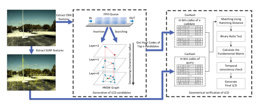
In this section a detailed description of the proposed LCD pipeline is presented. The algorithm leverages the GPU acceleration and HNSW graphs [21] to achieve real-time performance. The whole process can be summarized as two stages: the generation of LCD candidates and the verification of LCD.
In the first stage, a HNSW graph is built and retrieved using CNN features, which is extracted from the incoming frames. Using a First-in-First-out (FIFO) queue, the recently captured images can be filtered out in the retrieval process. We carefully choose a highly efficient CNN model to extract features, which has an extremely fast speed on GPU. The use of HNSW ensures the building and the retrieval process of the database cost a few milliseconds.
In the second stage, SURF features are matched using CasHash [10] matcher followed by ratio test [12] and RANSAC to perform geometrical verification. We exploit the ratio test using Hamming distance instead of using the L2 distance of the original features, which will significantly save memory or disk space. The time-consuming process here is the extraction of SURF features. Therefore, we utilize GPU to accelerate it, which guarantee the high precision and rapid verification.
III-A Description of the Features
The proposed loop closure recognition system utilizes a lightweight Deep Convolution Neural Network named MobileNetV2 [22], which is based on an inverted residual structure with linear bottlenecks. MobileNetV2 allows very memory-efficient inferences which are suitable for mobile applications.
The CNN features are extracted using the final average pooling layer of MobileNetV2. The network architecture is simplified by merging the batch normalization layer with a preceding convolution [34]. The forwarding time will be decreased by adding this operation. The computational process can be written as:
| (1) |
Here and denote the weight matrix and bias of the normalized version of a feature map . The parameters of the convolution layer which precedes batch normalization are denoted as and , where is the number of channels of the feature map input to the convolutional layer and is the filter size. A neighborhood of is unwrapped in to a vector . Then the batch normalization layer and the preceding convolution layer can be replaced by a single convolution layer with the following parameters:
| (2) |
| (3) |
The local invariant feature used in our system is Speeded Up Robust Features (SURF) [13], which is based on the Hessian matrix to find points of interest. Circular regions around the interest points are constructed in order to assign a unique orientation and thus gain invariance to image rotations. In order to achieve higher accuracy, the proposed algorithm utilizes the full SURF space, which is 128 dimensions.
III-B Generation of LCD candidates
When the robot travels on the road, the camera mounted on it will capture images and extract CNN features using MobilenetV2 [22]. Then these features are used to build the HNSW graphs and perform the retrieval to generate loop closure candidates.
The similarity between the features is calculated using the normalized scalar product (cosine of the angle between vectors) [35]:
| (4) |
Where is the similarity score between images and , and and are the CNN feature vectors corresponding to the images. is the norm of vector .
Our system employs a proximity graph approach, called HNSW graphs [21], which outperforms the state-of-the-art approximate nearest neighbor search methods, such as tree based BoW [36] models, PQ [31] and LSH [37]. In the following sub-sections we describe HNSW s properties and explain how to use HNSW to construct graph vocabulary and perform approximate nearest neighbor search with the strategy to filter out the recently captured images.
III-B1 Properties of HNSW
The HNSW graph is a fully graph based incremental K-Nearest Neighbor Search (K-NNS) structure, as shown in Fig. 2. It is based on Navigable Small World (NSW) model [38], which has logarithmic or polylogarithmic scaling of greedy graph routing. Such models are important for understanding the underlying mechanisms of real-life networks formation.
The graph formally consists of a set of nodes (i.e. feature vectors) and a set of links between them. A link connects node with node , which is directed in HNSW. The neighborhood of a node is defined as the set of its immediately connected nodes. HNSW uses strategies for explicit selection of the graph s enter-point node, separate links by different scales and selecting neighbors using an advanced heuristic. The links are separated according to their length scale into different layers and then search in a hierarchical multilayer graph, which allows a logarithmic scalability.
III-B2 Construction of Graph Vocabulary
In a BoW model, the visual vocabulary is usually constructed using k-means clustering. A search index is built over the visual words, which are generated using feature descriptors extracted from a training dataset. The building of the vocabulary is off-line, which means that it is not flexible and can not adapt to every working environment.
HNSW has the property of incremental graph building [21]. The image features can be consecutively inserted into the graph structure. An integer maximum layer is randomly selected with an exponentially decaying probability distribution for every inserted element. The insertion process starts from the top layer to the next layer, by greedily traversing the graph in order to find the closest neighbors to the inserted element in the layer. The founded closest neighbors from the previous layer will be used as an enter point to the next layer. A greedy search algorithm is used to find closest neighbors in each layer. The process repeats until the connections of the inserted elements are established on the zero layer. In each layer higher than zero, the maximum number of connections that an element can have per layer is defined by the parameter , which is the only meaningful construction parameter.
During the movement of the mobile robot, the CNN features of the images are inserted into the graph vocabulary. The whole process is on-line and incremental, thus eliminating the need for prebuilt data. Therefore, the use of HNSW ensures the robot’s working in various environment.
III-B3 K-NN Search and Adaption for LCD
The K-NN Search algorithm is roughly equivalent to the insertion algorithm for an item with layer , with the difference that the closest neighbors found at the ground layer are returned as the search result. The search quality is controlled by the parameter .
The images are captured sequentially and the adjacent images may have high similarities, which will result in false-positive LCDs. Therefore, we design a First-in-First-out (FIFO) queue to store image features. The image feature of the current Image is first inserted into the queue and until the robot runs out of the search area the feature will be inserted into the HNSW graph. The search area that rejects recently acquired input frames is defined based on a temporal constant and the frame rate of the camera . If the frames feed into the queue more than , the insertion into the HNSW graph is performed, otherwise, it will only insert into the queue . Consequently, when we use the current feature as the query feature, it will only search in database, where is the number of entire images up to now. The features in the search area will never appear in the results.
III-C Geometrical verification of LCD
| Dataset | Description | Camera Position | Image Resolution | # Images | Frames Per Second |
|---|---|---|---|---|---|
| KITTI 00 [39] | Outdoor, dynamic | Frontal | 4541 | 10 | |
| KITTI 05 [39] | Outdoor, dynamic | Frontal | 2761 | 10 | |
| Malaga 2009 Parking 6L [11] | Outdoor, slightly dynamic | Frontal | 3474 | 7 | |
| New College [40] | Outdoor, dynamic | Frontal | 52480 | 20 |
Our system incorporates a geometrical verification step for discarding outliers by verifying that the two images of the loop closure satisfy the geometrical constraint. As said in Section II, we utilize the local SURF feature for image matching between a query and the top nearest neighbors. For verification, the fundamental matrix is computed using RANSAC, and then, the data association between the images can be derived with no extra cost, which can be used for any SLAM algorithm.
Here, we use the CasHash [10] algorithm for pairwise image matching. The initial purpose of CasHash is rapid image matching for 3D reconstruction. The features of images are mapped into binary codes from coarse to fine. It uses hashing tables which have bits, and then each feature is assigned to a bucket . The functions are represented in Eqn.5, where are generated independently and uniformly at random from a locality sensitive family :
| (5) |
The original SURF feature has 128D float-point descriptors, while using the CasHash the features can be changed to binary codes with bits. In the traditional use of CasHash, a ratio test is performed using the full feature space. However, in the application for a mobile robot, the memory of the mounted computer of the robot is limited. The cost of saving all SURF features of all frames is not practical. We propose that using the binary codes instead of the full features for the ratio test. The binary ratio test threshold is defined as:
| (6) |
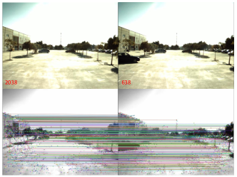
Here indicates the Hamming distance computation. are the binary codes of the descriptor in an image , while and are the binary codes of two closest descriptors and in an image . The feature matches which have lower ratio than will be treated as good matches and feed into the RANSAC process to estimated a fundamental matrix between the query and the loop closure candidate images. In Fig. 1, a representation of the image matching is shown, which use the binary ratio test and RANSAC to remove outliers.
The loop closure candidate is ignored if it fails to compute or the number of inlier points between the two images is less than a parameter . A temporal consistency check is incorporated to examine whether the aforementioned conditions are met for the consecutive camera measurements, which is the same as the method used in [9].
After the CasHash, each feature is encoded as bit hashing codes. For example, if we use , which equate to 128 bits in the hashing, the memory usage will decrease from 128 floats to 128 bits, which means it only cost memory. This feature is very important in mobile robot applications, which have less memory than the servers.
IV EXPERIMENTAL EVALUATION
The evaluation datasets contain four publicly available image sets: KITII 00 [39], KITTI 05 [39], Malaga 2009 Parking 6L [11] and New College [40]. A more detailed description of the datasets can be seen in Table I. The ground truth of these datasets are provided by the authors in [9] and the authors in [8]. The performance of our method is compared against the state-of-the-art methods such as, FAB-MAP 2.0 [23],IBuILD [26],Bampis et al. [24], Gehrig et al. [17], Glvez-Lpez et al. [8], Tsintotas et al. [9].
IV-A Method Evaluation
We train the CNN network using the Place365 [41] dataset, which has 10 million images and 365 classes of scene for scene recognition. The top 1 accuracy is 51.47% and top 5 accuracy is 82.61%. We use this model in the following experiments.
The parameters of our method include three parts: the parameters of SURF features, HNSW graph, and geometrical verification. We use the default parameters of SURF, because it is not the research emphasis of this paper. An implementation of the loop closure detection algorithm presented in this paper is distributed as an open source code.
For HNSW graph construction and searching, there are two parameters that could affect the search quality: the number of nearest to elements to return, ; and the maximum number of connections for each element per layer, . The range of the parameter should be within 200, because the increase in will lead to little extra performance but in exchange, significantly longer construction time. The range of the parameter should be 5 to 48. The experiments in [21] show that bigger is better for high recall and high dimensional data, which also defines the memory consumption of the algorithm. The temporal constant using in the FIFO queue will be set to 40 seconds in the rest of the paper. For geometrical verification, the parameters are: the hashing bits , the ratio for binary ratio test , and the returned number of nearest neighbors . The inlier points threshold is set to 20 empirically.
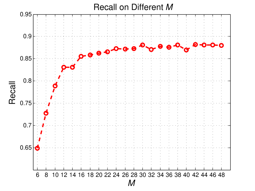
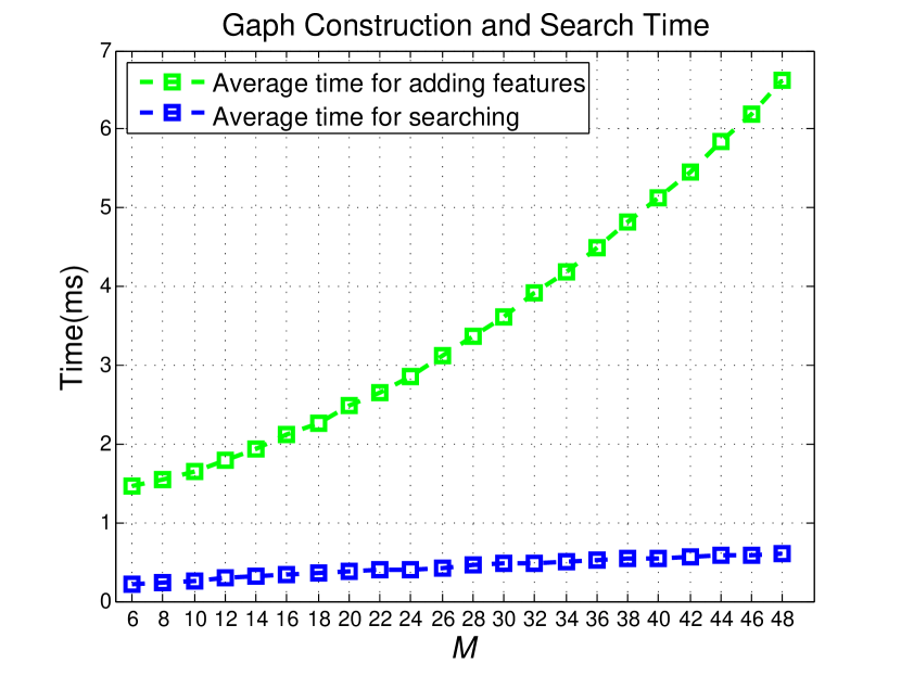
Firstly, we perform the experiments on the New College dataset[40] to choose and for the HNSW graph retrieval. The other parameters are set as: , . is set to 200 when we change . The returned number of nearest neighbors is set to 1. As 100% precision can be reached with the temporal consistency check. The recalls are shown in the left part of Fig. 3. We can see when increase, the recall will also increase. In the right part of Fig. 3, the feature adding time and searching time will be increased when increases.
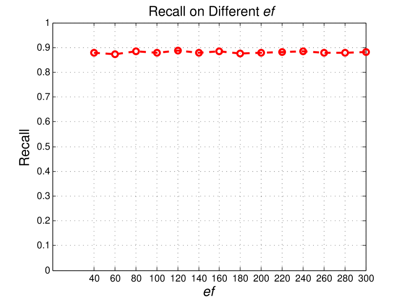
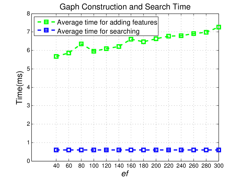
To evaluate different , the parameter is set to 16. It can be seen that in the left part of Fig. 4, the recall does not significantly change when the increases. In the right part of Fig. 4, the feature adding time will be increased when increases, while the searching time remains with no growth. According to the recall curve in Fig. 3 and Fig. 4, we chose and in the following experiments.
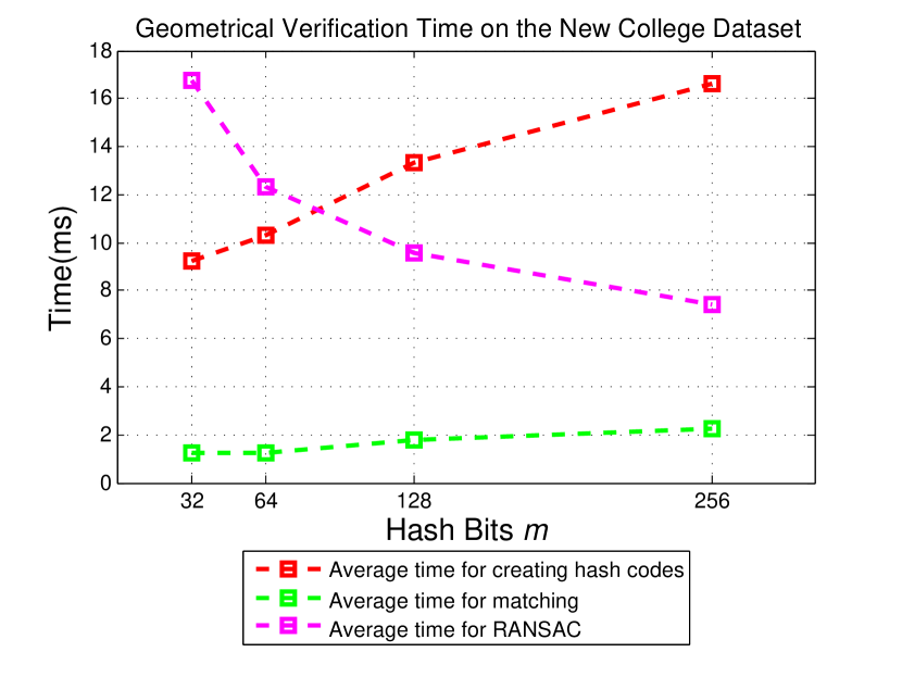
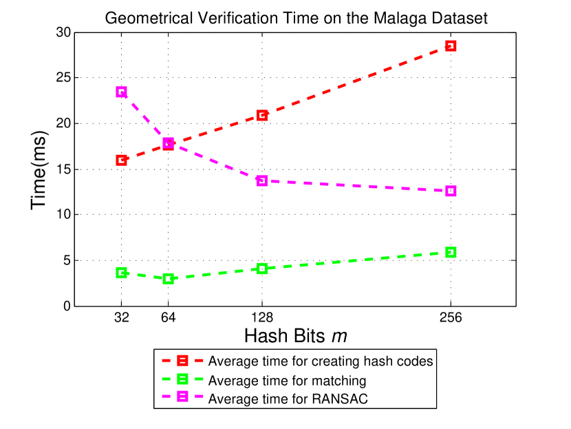
Secondly, the hashing bits and the ratio are evaluated. To evaluate the hash bits , the ratio are set as . The returned number of nearest neighbors is set to 1. The temporal consistency check is incorporated in these experiments. The recalls of New College dataset and Malaga dataset are shown in Table II and Table III. It can be seen that using more hashing bits will increase the recall. In the Fig. 5, we can see that the hash codes creating time and the matching time will be increased when the hash bits increase, while the RANSAC time will be decreased. We chose in the remaining experiments, because the increase of the time is acceptable and the recall is better.
| Different Hashing Bits | 32 | 64 | 128 | 256 |
|---|---|---|---|---|
| Recall (%) | 87.83 | 88.30 | 89.34 | 90.67 |
| Precision (%) | 100.0 | 100.0 | 100.0 | 100.0 |
| Different Hashing Bits | 32 | 64 | 128 | 256 |
|---|---|---|---|---|
| Recall (%) | 87.92 | 82.72 | 82.38 | 85.23 |
| Precision (%) | 90.81 | 97.82 | 99.59 | 99.80 |
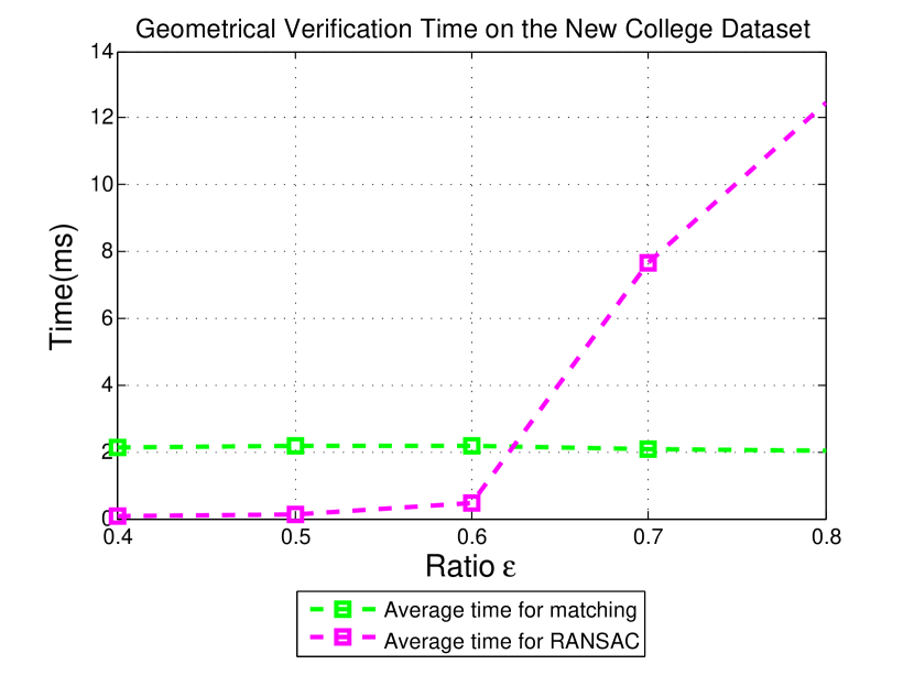
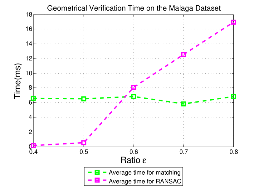
The ratio of the binary ratio test is also very important for the precision and the recall of our system. We set , and the temporal consistency check is used to evaluate the ratio. The recalls of New College dataset and Malaga dataset will increase as the ratio increases, as shown in Table IV and Table V. The hash matching time will not increase during the change of the ratio, while the RANSAC time will be increased significantly, as shown in Fig. 6. We chose to ensure the precision to be 100% and to achieve a higher recall.
| Ratio of Binary Ratio Test | 0.4 | 0.5 | 0.6 | 0.7 | 0.8 |
|---|---|---|---|---|---|
| Recall (%) | 30.84 | 57.57 | 78.42 | 88.73 | 92.35 |
| Precision (%) | 100.0 | 100.0 | 100.0 | 100.0 | 100.0 |
| Ratio of Binary Ratio Test | 0.4 | 0.5 | 0.6 | 0.7 | 0.8 |
|---|---|---|---|---|---|
| Recall (%) | 43.22 | 55.34 | 67.78 | 81.82 | 92.98 |
| Precision (%) | 100.0 | 100.0 | 100.0 | 100.0 | 97.49 |
Finally, the returned number of nearest neighbors is evaluated. We can see in the Table VI and Table VII, the recall will be increased when the increased. For the Malaga dataset [11], the recall is 80.54% at 100% precision when it returned the nearest neighbor, while increasing will cause a decrease in precision. Because the 100% precision is important for the loop closure detection, we selected . Using more nearest neighbor in the geometrical verification stage will cost more time for hash code matching and RANSAC. Therefore, using only the nearest neighbor will bring a reduction in processing time. According to the above experiments, we determine the parameters of our algorithm, which are summarized in Table VIII.
| Nearest Neighbors | 1 | 2 | 4 | 6 | 8 | 10 |
|---|---|---|---|---|---|---|
| Recall (%) | 89.94 | 94.85 | 97.67 | 97.76 | 97.85 | 98.41 |
| Precision (%) | 100.0 | 100.0 | 100.0 | 100.0 | 100.0 | 100.0 |
| Nearest Neighbors | 1 | 2 | 4 | 6 | 8 | 10 |
|---|---|---|---|---|---|---|
| Recall (%) | 80.54 | 89.19 | 97.95 | 96.69 | 97.33 | 96.49 |
| Precision (%) | 100.0 | 99.82 | 99.36 | 99.23 | 99.24 | 99.25 |
IV-B Comparative Results
In the Table X, the precision and recall of the proposed method against the aforementioned state-of-the-art methods are compared. The best, second and third best results are marked in red, blue and green, respectively. Our method best in the New College dataset, 2 points higher than Tsintotas et al. [9]. In the Malaga dataset, our method achieved 80.54% recall at 100% precision, which is lower than Tsintotas’ method [9] and was second best. For KITTI 00 and KITTI 05 dataset, our method was higher than Bampis’s method [24].
IV-C Execution Time and Memory Usage
We evaluated the feature extraction time on the GPU. The forwarding time of MobileNetV2 [22] was 13.33 ms, while the forwarding time of merging the batch normalization layer was 5.35 ms, which achieve an obvious speed acceleration.
To measure the execution time of whole system, we ran our system using the New College dataset [40] using the parameters in Table VIII. The first experiment used the working frequency , which processed a total of 2624 images. The execution time of our system cost 48.73 ms per image on average and a peak of 83.70 ms. In order to test the scalability of the system, we set the frequency to and obtained 52480 images. The execution time consumed per image in that case is shown in Table IX. This was measured on a Intel(R) Xeon(R) CPU E5-2640 v4 @ 2.40GHz machine, with a NVIDIA P40 GPU card. The average running time per image was about 50 ms, which is very close to that using 2624 images and fast enough for loop closure detection. The average running time of Tsintotas’s method [9] is about 300 ms, which is 6 times higher than our method.
| Number of nearest to elements to return, | 40 |
| Maximum number of connections for each element per layer, | 48 |
| Search area time constant, | 40 |
| Hashing bits, | 256 |
| Ratio of binary ratio test, | 0.7 |
| Geometrical verification inliers, | 20 |
| Images temporal consistency, | 2 |
| Number of returned nearest neighbors, | 1 |
As described in section III-C, we use CasHash [10] for image matching, which quantize the SURF features into binary hashing codes. The proposed binary ratio test can avoid having to save the full float-point features. The memory usage of using full float-point features in our system is 28.11 GB, while using hashing codes only cost 18.99 GB, which saves 32% of memory usage.
| Stages | Mean Time (ms/query) |
|---|---|
| CNN Feature Extraction | 8.72 |
| SURF Feature Extraction | 8.97 |
| Hash Codes Creation | 16.94 |
| Adding CNN Feature | 5.21 |
| Graph Searching | 0.93 |
| Hash Codes Matching | 2.23 |
| RANSAC | 7.55 |
| Whole System | 50.28 |
| Dataset | Approaches | Precision (%) | Recall (%) |
| KITTI 00 [39] | Gehrig et al. [17] | 100 | 92 |
| Bampis et al. [24] | 100 | 81.54 | |
| Tsintotas et al. [9] | 100 | 93.18 | |
| FILD | 100 | 91.23 | |
| KITTI 05 [39] | Gehrig et al. [17] | 100 | 94 |
| Bampis et al. [24] | 100 | 84.80 | |
| Tsintotas et al. [9] | 100 | 94.20 | |
| FILD | 100 | 85.15 | |
| Malaga 2009 Parking 6L [11] | Glvez-Lpez et al. [8] | 100 | 74.75 |
| FAB-MAP 2.0 [23] | 100 | 68.52 | |
| Bampis et al. [24] | 100 | 76.78 | |
| IBuILD [26] | 100 | 78.13 | |
| Tsintotas et al. [9] | 100 | 87.99 | |
| FILD | 100 | 80.54 | |
| New College [40] | Glvez-Lpez et al. [8] | 100 | 55.92 |
| Bampis et al. [24] | 100 | 77.55 | |
| Tsintotas et al. [9] | 100 | 87.97 | |
| FILD | 100 | 89.94 |
IV-D Discussion
The performance of our system depends on several factors: the classification accuracy of the CNN model, the retrieval precision and recall of the HNSW graphs, and the effectiveness of the geometrical verification. In this case, the CNN features were extracted using the final average pooling layer of MobileNetV2. An increase in the classification accuracy will lead to an increase of recall in the whole LCD system. For example, we tested our system using the ResNet152 model provided by the author in [41]. The recall at 100% precision for the New College dataset was 93.85%, which was higher than our result of 89.94%. The reason why we have not used ResNet152 was that it cost more time in forwarding time, about 135 ms in GPU, which is intolerable for mobile robot applications. In the future, we will try to improve the classification accuracy using the Place365 [41] dataset. The performance of different parameters of the HNSW graphs were exhaustively evaluated. However, we did not fully utilize the similarity scores of the query and the returned images. A proper threshold may have helped us eliminate false positives. In the geometrical verification step, the hashing bits and the ratio are important for the recall and the processing time. We plan to accelerate the CasHash [10] algorithm using hardware instruction set or optimized math functions, which should enable us to use more bits to achieve higher recall with suitable time costs.
V CONCLUSIONS
In this paper, an online, incremental approach for fast loop closure detection is presented. The proposed method is based on the GPU computed features and HNSW graph vocabulary construction. A novel geometrical verification method based on hashing codes is introduced, which is coupled with binary ratio test to generate loop closure. The approach is evaluated on different publicly available outdoor datasets, and the results show that it achieve fairly good results compared with other state-of-the-art methods, which is capable of generating higher recall at 100% precision.
VI ACKNOWLEDGMENTS
The authors would like to thank Dr. Konstantinos A. Tsintotas for kindly offering GT information for the datasets, and Dr. Cong Leng for the constructive suggestion.
References
- [1] H. Durrant-Whyte and T. Bailey, “Simultaneous localization and mapping: part i,” IEEE Robotics & Automation Magazine, vol. 13, no. 2, pp. 99–110, 2006.
- [2] T. Bailey and H. Durrant-Whyte, “Simultaneous localization and mapping (slam): Part ii,” IEEE Robotics & Automation Magazine, vol. 13, no. 3, pp. 108–117, 2006.
- [3] J.-S. Gutmann and K. Konolige, “Incremental mapping of large cyclic environments,” in Computational Intelligence in Robotics and Automation, Proceedings. 1999 IEEE International Symposium on. IEEE, 1999, pp. 318–325.
- [4] J. D. Tardós, J. Neira, P. M. Newman, and J. J. Leonard, “Robust mapping and localization in indoor environments using sonar data,” The International Journal of Robotics Research, vol. 21, no. 4, pp. 311–330, 2002.
- [5] M. Cummins and P. Newman, “Fab-map: Probabilistic localization and mapping in the space of appearance,” The International Journal of Robotics Research, vol. 27, no. 6, pp. 647–665, 2008.
- [6] J. Engel, J. Stückler, and D. Cremers, “Large-scale direct slam with stereo cameras,” in Intelligent Robots and Systems (IROS), 2015 IEEE/RSJ International Conference on. IEEE, 2015, pp. 1935–1942.
- [7] A. Angeli, D. Filliat, S. Doncieux, and J.-A. Meyer, “Fast and incremental method for loop-closure detection using bags of visual words,” IEEE Transactions on Robotics, vol. 24, no. 5, pp. 1027–1037, 2008.
- [8] D. Gálvez-López and J. D. Tardos, “Bags of binary words for fast place recognition in image sequences,” IEEE Transactions on Robotics, vol. 28, no. 5, pp. 1188–1197, 2012.
- [9] K. A. Tsintotas, L. Bampis, and A. Gasteratos, “Assigning visual words to places for loop closure detection,” in 2018 IEEE International Conference on Robotics and Automation (ICRA). IEEE, 2018, pp. 1–7.
- [10] J. Cheng, C. Leng, J. Wu, H. Cui, and H. Lu, “Fast and accurate image matching with cascade hashing for 3d reconstruction,” in Proceedings of the IEEE Conference on Computer Vision and Pattern Recognition, 2014, pp. 1–8.
- [11] J.-L. Blanco, F.-A. Moreno, and J. Gonzalez, “A collection of outdoor robotic datasets with centimeter-accuracy ground truth,” Autonomous Robots, vol. 27, no. 4, p. 327, 2009.
- [12] D. G. Lowe, “Distinctive image features from scale-invariant keypoints,” International Journal of Computer Vision, vol. 60, no. 2, pp. 91–110, 2004.
- [13] H. Bay, T. Tuytelaars, and L. Van Gool, “Surf: Speeded up robust features,” in European Conference on Computer Vision. Springer, 2006, pp. 404–417.
- [14] M. Calonder, V. Lepetit, C. Strecha, and P. Fua, “Brief: Binary robust independent elementary features,” in European Conference on Computer Vision. Springer, 2010, pp. 778–792.
- [15] E. Rublee, V. Rabaud, K. Konolige, and G. Bradski, “Orb: An efficient alternative to sift or surf,” in Computer Vision (ICCV), 2011 IEEE International Conference on. IEEE, 2011, pp. 2564–2571.
- [16] J. Sivic and A. Zisserman, “Video google: A text retrieval approach to object matching in videos,” in Computer Vision (ICCV), 2003 IEEE International Conference on. IEEE, 2003, p. 1470.
- [17] M. Gehrig, E. Stumm, T. Hinzmann, and R. Siegwart, “Visual place recognition with probabilistic voting,” Robotics and Automation (ICRA), 2017 IEEE International Conference on, pp. 3192–3199, 2017.
- [18] A. Krizhevsky, I. Sutskever, and G. E. Hinton, “Imagenet classification with deep convolutional neural networks,” in Advances in Neural Information Processing Systems, 2012, pp. 1097–1105.
- [19] B. Zhou, A. Lapedriza, J. Xiao, A. Torralba, and A. Oliva, “Learning deep features for scene recognition using places database,” in Advances in Neural Information Processing Systems, 2014, pp. 487–495.
- [20] N. Sünderhauf, S. Shirazi, A. Jacobson, F. Dayoub, E. Pepperell, B. Upcroft, and M. Milford, “Place recognition with convnet landmarks: Viewpoint-robust, condition-robust, training-free,” Proceedings of Robotics: Science and Systems XII, 2015.
- [21] Y. A. Malkov and D. A. Yashunin, “Efficient and robust approximate nearest neighbor search using hierarchical navigable small world graphs,” IEEE Transactions on Pattern Analysis and Machine Intelligence, 2018.
- [22] M. Sandler, A. Howard, M. Zhu, A. Zhmoginov, and L.-C. Chen, “Mobilenetv2: Inverted residuals and linear bottlenecks,” in 2018 IEEE/CVF Conference on Computer Vision and Pattern Recognition. IEEE, 2018, pp. 4510–4520.
- [23] M. Cummins and P. Newman, “Appearance-only slam at large scale with fab-map 2.0,” The International Journal of Robotics Research, vol. 30, no. 9, pp. 1100–1123, 2011.
- [24] L. Bampis, A. Amanatiadis, and A. Gasteratos, “Encoding the description of image sequences: A two-layered pipeline for loop closure detection,” in Intelligent Robots and Systems (IROS), 2016 IEEE/RSJ International Conference on. IEEE, 2016, pp. 4530–4536.
- [25] T. Nicosevici and R. Garcia, “Automatic visual bag-of-words for online robot navigation and mapping,” IEEE Transactions on Robotics, vol. 28, no. 4, pp. 886–898, 2012.
- [26] S. Khan and D. Wollherr, “Ibuild: Incremental bag of binary words for appearance based loop closure detection,” in Robotics and Automation (ICRA), 2015 IEEE International Conference on. IEEE, 2015, pp. 5441–5447.
- [27] A. Torralba, K. P. Murphy, W. T. Freeman, M. A. Rubin et al., “Context-based vision system for place and object recognition.” in Computer Vision (ICCV), 2003 IEEE International Conference on, vol. 3, 2003, pp. 273–280.
- [28] N. Sünderhauf, S. Shirazi, F. Dayoub, B. Upcroft, and M. Milford, “On the performance of convnet features for place recognition,” in Intelligent Robots and Systems (IROS), 2015 IEEE/RSJ International Conference on. IEEE, 2015, pp. 4297–4304.
- [29] Y. Hou, H. Zhang, and S. Zhou, “Convolutional neural network-based image representation for visual loop closure detection,” in Information and Automation, 2015 IEEE International Conference on. IEEE, 2015, pp. 2238–2245.
- [30] Y. Liu and H. Zhang, “Indexing visual features: Real-time loop closure detection using a tree structure,” in Robotics and Automation (ICRA), 2012 IEEE International Conference on. IEEE, 2012, pp. 3613–3618.
- [31] H. Jegou, M. Douze, and C. Schmid, “Product quantization for nearest neighbor search,” IEEE Transactions on Pattern Analysis and Machine Intelligence, vol. 33, no. 1, pp. 117–128, 2011.
- [32] Y. Hou, H. Zhang, and S. Zhou, “Bocnf: Efficient image matching with bag of convnet features for scalable and robust visual place recognition,” Autonomous Robots, vol. 42, no. 6, pp. 1169–1185, 2018.
- [33] K. Hajebi and H. Zhang, “An efficient index for visual search in appearance-based slam,” in Robotics and Automation (ICRA), 2014 IEEE International Conference on. IEEE, 2014, pp. 353–358.
- [34] (2018) Fusing batch normalization and convolution in runtime. [Online]. Available: https://tkv.io/posts/fusing-batchnorm-and-conv/
- [35] J. Sivic, “Efficient visual search of images videos,” University of Oxford, 2006.
- [36] M. Muja and D. G. Lowe, “Scalable nearest neighbor algorithms for high dimensional data,” IEEE Transactions on Pattern Analysis & Machine Intelligence, no. 11, pp. 2227–2240, 2014.
- [37] A. Andoni and I. Razenshteyn, “Optimal data-dependent hashing for approximate near neighbors,” in Proceedings of the forty-seventh annual ACM symposium on Theory of computing. ACM, 2015, pp. 793–801.
- [38] J. M. Kleinberg, “Navigation in a small world,” Nature, vol. 406, no. 6798, p. 845, 2000.
- [39] J. Fritsch, T. Kuehnl, and A. Geiger, “A new performance measure and evaluation benchmark for road detection algorithms,” in 16th International IEEE Conference on Intelligent Transportation Systems (ITSC 2013). IEEE, 2013, pp. 1693–1700.
- [40] M. Smith, I. Baldwin, W. Churchill, R. Paul, and P. Newman, “The new college vision and laser data set,” The International Journal of Robotics Research, vol. 28, no. 5, pp. 595–599, 2009.
- [41] B. Zhou, A. Lapedriza, A. Khosla, A. Oliva, and A. Torralba, “Places: A 10 million image database for scene recognition,” IEEE transactions on pattern analysis and machine intelligence, vol. 40, no. 6, pp. 1452–1464, 2018.