The Tilted Beta Binomial Linear Regression Model: a Bayesian Approach

Abstract

This paper proposes new linear regression models to deal with overdispersed binomial datasets. These new models, called tilted beta binomial regression models, are defined from the tilted beta binomial distribution, proposed assuming that the parameter of the binomial distribution follows a tilted beta distribution. As a particular case of this regression models, we propose the beta rectangular binomial regression models, defined from the binomial distribution assuming that their parameters follow a beta rectangular distribution. These new linear regression models, defined assuming that the parameters of these new distributions follow regression structures, are fitted applying Bayesian methods and using the OpenBUGS software. The proposed regression models are fitted to an overdispersed binomial dataset of the number of seeds that germinate depending on the type of chosen seed androot.

Key words: Count data, overdispersion, tilted beta distribution, binomial distribution, tilted beta binomial distribution, Bayesian approach.

1 Introduction

The binomial distribution is normally used to model the number of successes obtained in a finite number of experiments. However, in these cases, it is often found that the variance of the response variable $Y$ exceeds the theoretical variance of the binomial distribution. This phenomenon, known as extra-binomial variation (overdispersion), can lead to underestimation errors, lost efficiency of estimates and underestimation of the variance, wich that can in turn generate incorrect inferences about the regression parameters or the credible intervals (Williams,, 1982; Cox,, 1983; Collet,, 1991).

There are several approaches to study overdispersed binomial datasets. Hinde and Demétrio, (1998) categorized the majority of overdispersed binomial models in two classes: (1) those in which a more general shape for the variance function is assumed, by adding additional parameters; and (2) models in which it is assumed that the parameter of the distribution of the response variable is itself a random variable. In the first class, the double exponential family of distributions allows the researcher to obtain double binomial models, which allow including a second parameter, which independently from the mean controls for the variance of the response variable and can be modeled from a subset of some explanatory variables (Efron,, 1986). In the second class, the beta binomial distribution, results by assuming that the response variable follows a binomial distribution and the probability parameter of the binomial distribution follows a beta distribution. From the parameterization of the beta distribution, in terms of its mean and dispersion parameter (Jorgensen,, 1997), a parameterization of the beta binomial beta distribution in terms of its mean and dispersion parameters is presented in Cepeda-Cuervo and Cifuentes-Amado, (2017).

Despite the versatility of the beta distribution, Hahn, (2008) proposed the rectangular beta distribution as a combination between the beta distribution and the uniform distribution, to admit heavier tails than that admitted by the beta distribution. After that, Hahn and López Martín, (2015) introduced tilted beta distribution, which has as particular cases the beta rectangular and the beta distributions.

In this article, we generalize the beta binomial regression models for fitting overdispersed binomial count dataset (Cepeda-Cuervo and Cifuentes-Amado,, 2017) by introducing the tilted beta binomial linear regression model. For this, the tilted beta binomial probability is defined by assuming that the parameter of the binomial distribution follows the mean tilted beta distribution. In addition, the beta rectangular binomial models are presented as particular cases of the new proposed model, by assuming that the parameter of the binomial distribution has beta rectangular distribution. The proposed models are fitted using Bayesian methods. Finally, in order to illustrate of the tilted beta binomial model, we fit it to a seed germination count dataset and compare it with the rectangular beta binomial model and the binomial model, using their DIC values.

This paper is organized as follows. After the introduction, in Section 2, the tilted and the reparameterized tilted beta distributions are presented. In Section 3, the tilted beta binomial distribution is introduced and the rectangular beta binomial distribution is presented as a particular case. In Section 4, the tilted beta binomial linear regression model is defined. Finally, in Section 5, we analyze how the proportion of seeds that germinated on each of 21 dishes, is influenced by the type of seed and root, by fitting a tilted beta binomial linear regression, using the OpenBUGS software. The proposed model performance is compared with the binomial and beta binomial regression models.

2 The Tilted Beta Distribution

In different fields there is often a need to model continuous random variables that assume values in a bounded interval on a set of explanatory variables. Cepeda-Cuervo, (2001) proposed the beta regression models, where mean and dispersion parameters follow regression structures (see also Cepeda and Gamerman, (2005), Cepeda-Cuervo and Garrido, (2015)). If the continuous variable $Y$ assumes values in a bounded open interval $(a,b)$, a beta regression models can be proposed, using the basic transformation $(y-a)/(b-a)$. However, in order to admit heavier tails than is possible in the beta distribution, Hahn, (2008) proposed the rectangular beta distribution as a new distribution that, like the beta distribution, has as domain the open interval $(0,1)$. The rectangular beta distribution consists of convex combination between the beta distribution and the uniform distribution $U(0,1)$. Subsequently Hahn and López Martín, (2015), proposed the tilted beta distribution, consisting of a mixture of the beta distribution and the tilted distribution, which has as particular cases the beta rectangular distribution and the beta distribution. This section presents a reparameterization of the tilted beta distribution proposed by Hahn and López Martín, (2015), in terms of the mean and the dispersion parameters of the beta distribution $\mu_{b}$ and $\phi$, respectively, and the mean of the tilted beta distribution $\mu_{t}$. The ($\mu_{t}$,$\mu_{b}$,$\phi$,$\theta$)-tilted beta binomial distribution results from the convex combination between the tilted reparameterized beta distribution and the binomial distribution.

2.1 The Tilted Distribution

A random variable $Y$ follows an inclined distribution with a parameter $\nu$ (Hahn and López Martín,, 2015) if its density is given by:

$$c(y|\nu)=\left[2\nu-2(2\nu-1)y\right]I_{(0,1)(y)},\quad 0\leq\nu\leq 1$$ (1)

The mean of $Y$, denoted $\mu_{t}:=E(Y|\nu)$, is equal to $\mu_{t}=(2-\nu)/3$. By reparameterizing (1) in terms of the mean, the density function is defined by:

$$c(y|\mu_{t})=\left[3(2\mu_{t}-1)(2y-1)+1\right]I_{(0,1)(y)},$$ (2)

where $1/3\leq\mu_{t}\leq 2/3$, given that the moments, $E_{t}(Y^{n})$, of a random variable $Y$ which follows the density function (2) are given by:

$$E_{t}(Y^{n}) =\int_{0}^{1}y^{n}\left[3(2\mu_{t}-1)(2y-1)+1\right]dy$$

$$=\frac{3n(2\mu_{t}-1)+n+2}{(n+1)(n+2)},\;\;n=1,2,...$$ (3)

Their variance, $V_{t}(Y)$, is given by:

$$V_{t}(Y) =\frac{6(2\mu_{t}-1)+4}{12}-\mu_{t}^{2}$$

$$=\mu_{t}(1-\mu_{t})-\frac{1}{6}.$$

2.2 Reparameterized Tilted Beta Distribution

The tilted beta distribution was introduced by Hahn and López Martín, (2015), as the convex combination between the tilted distribution and the beta distribution. If this distribution is obtained from the combination of the mean tilted distribution (2) and the mean and the dispersion beta distribution, $Beta(\mu_{b},\phi)$, the density function of the tilted beta distribution is given by (4):

$$f(y|\mu_{t},\mu_{b},\phi,\theta)=\theta c(y|\mu_{t})+(1-\theta)f_{Beta}(y|\mu_{b},\phi)$$ (4)

where $0\leq\theta\leq 1$. The notation $Y\sim BI(\mu_{t},\mu_{b},\phi,\theta)$ is used to denote that $Y$ follows a tilted beta distribution. Since the $n$-th-moment of $Y$ is given by:

$$E(Y^{n}) =\int^{1}_{0}y^{n}\theta c(y|\mu_{t})dy+\int^{1}_{0}y^{n}(1-\theta)f_{Beta}(y|\mu_{b})dy$$

$$=\theta E_{t}(Y^{n})+(1-\theta)E_{b}(Y^{n})$$

$$=\theta\frac{3n(2\mu_{t}-1)+n+2}{(n+1)(n+2)}+(1-\theta)\frac{\Gamma(\mu_{b}\phi+n)\Gamma(\phi)}{\Gamma(\mu_{b}\phi)\Gamma(\phi+n)},$$ (5)

the mean and the variance of the tilted beta distribution are:

$$E\left(Y|\mu_{t},\mu_{b},\phi,\theta\right) =\theta\mu_{t}+(1-\theta)\mu_{t}$$ (6)

$$V\left(Y|\mu_{t},\mu_{b},\phi,\theta\right) =E(Y^{2}|\mu_{t},\mu_{b},\phi,\theta)-E(Y|\mu_{t},\mu_{b},\phi,\theta)^{2}$$

$$=\left[\theta E_{(}Y^{2})+(1-\theta)E_{b}(Y^{2})\right]-\left[\theta\mu_{t}+(1-\theta)\mu_{b}\right]^{2}$$

$$=\theta V_{t}(Y)+(1-\theta)V_{b}(Y)+\theta\mu_{t}^{2}+(1-\theta)\mu_{b}^{2}-\left[\theta\mu_{t}+(1-\theta)\mu_{b}\right]^{2}$$

$$=\theta V_{t}(Y)+(1-\theta)V_{b}(Y)+\theta(1-\theta)(\mu_{t}+\mu_{b})^{2}$$ (7)

The rectangular beta distribution (Hahn,, 2008) is a particular case of (4) when $\mu_{t}=0.5$ (the slope of the tilted distribution is zero). By replacing this value of $\mu_{t}=o$ in (4), the density function of the tilted beta distributions is defined by:

$$f(y|\mu,\phi,\theta)=\theta+(1-\theta)f_{Beta}(y|\mu,\phi).$$ (8)

3 ($\mu_{t}$,$\mu_{b}$,$\phi$,$\theta$) - Tilted Beta Binomial Distribution

Let $Y|p\sim Bin(m,p)$ be a random variable that follows the binomial distribution, where $p$ follows the tilted beta distribution, $p\sim BI(\mu_{t},\mu_{b},\phi,\theta)$. Then $Y$ follows a tilted beta binomial distribution with parameters $\mu_{t}$, $\mu_{b}$, $\phi$ and $\theta$, denoted by $Y\sim BIB(\mu_{t},\mu_{b},\phi,\theta)$. The probability of this distribution is given by:

$$f(y|\mu_{t},\mu_{b},\phi,\theta) =\int_{0}^{1}f_{Bin}(y|m,p)\left[\theta c(p|\mu_{t})+(1-\theta)f_{Beta}(p|\mu_{b},\phi)\right]dp$$

$$=\left(\begin{array}[]{c}m\\ y\end{array}\right)\left[\theta\int_{0}^{1}[3(2\mu_{t}-1)(2p-1)+1]p^{y}(1-p)^{m-y}dp+\frac{(1-\theta)\Gamma(\phi)}{\Gamma(\mu_{b}\phi)\Gamma(\phi(1-\mu_{b}))}\right.$$ (11)

$$*\left.\int_{0}^{1}p^{y+\mu_{b}\phi-1}(1-p)^{m-y+\phi(1-\mu_{b})-1}dp\right]$$

$$=\theta\left(\begin{array}[]{c}m\\ y\end{array}\right)\left[(12\mu_{t}-6)\int_{0}^{1}p^{y+1}(1-p)^{m-y}dp+(-6\mu_{t}+4)\int_{0}^{1}p^{y}(1-p)^{m-y}dp\right]$$ (14)

$$+(1-\theta)f_{BB(\mu_{b},\phi)}(y|\mu_{b},\phi)$$

$$=2\theta\left(\begin{array}[]{c}m\\ y\end{array}\right)\left[(6\mu_{t}-3)\frac{y+1}{y+1+m-y+1}+(-3\mu_{t}+2)\right]B(y+1,m-y+1)$$ (17)

$$+(1-\theta)f_{BB(\mu_{b},\phi)}(y|\mu_{b},\phi)$$

$$=2\theta\left(\begin{array}[]{c}m\\ y\end{array}\right)\left[\frac{y(6\mu_{t}-3)+m(2-3\mu_{t})+1}{m+2}\right]B(y+1,m-y+1)+(1-\theta)f_{BB(\mu_{b},\phi)}(y),$$ (20)

where $B(\cdot,\cdot)$ denotes the beta function and $f_{BB(\mu_{b},\phi)}(\cdot)$ denotes the probability function of the beta binomial distribution, parameterized in terms of the mean and the dispersion parameters.

The behavior of the ($\mu_{t},\mu_{b},\phi,\theta$)-tilted beta binomial probability function is illustrated in Figure 1, for different vectors of parameter values:

Figure 1: Density function of the ($\mu_{t},\mu_{b},\phi,\theta$)-tilted beta binomial distribution.

The mean and variance of a random variable $Y$ that follows the ($\mu_{t},\mu_{b},\phi,\theta$)-tilted beta binomial probability function are given by:

$$E(Y) =E(E(Y|p))=mE(p)$$

$$=m\left[\theta\mu_{t}+(1-\theta)\mu_{b}\right]$$

$$V(Y) =V(E(Y|p))+E(V(Y|p))$$

$$=m^{2}V(p)+mE(p)-mE(p^{2}))$$

$$=m\left\{(m-1)V(p)+E(p)(1-E(p))\right\}$$

$$=m\left\{(m-1)\left[\theta V_{t}+(1-\theta)V_{b}+\theta(1-\theta)(\mu_{t}+\mu_{b})^{2}\right]+\left[\theta\mu_{t}+(1-\theta)\mu_{b}\right]\left[1-\theta\mu_{t}+(1-\theta)\mu_{b}\right]\right\}$$

where $\mu_{b}$, $V_{b}$ denote the mean and variance of the beta distribution, respectively, and $\mu_{t}$, $V_{t}$ denote the mean and variance of the tilted beta distribution.

3.1 ($\mu_{b}$,$\phi$,$\theta$)-Beta Rectangular Binomial Distribution

Let $Y|p\sim Bin(m,p)$ be a random variable that follows the binomial distribution, where $p$ follows the beta rectangular distribution (8). Thus, $Y$ follows the ($\mu_{b}$,$\phi$,$\theta$)-beta rectangular binomial distribution. This density function can be obtained as a particular case of the tilted beta binomial distribution (20), by replacing $\mu_{t}$ by $0.5$:

$$f(y|\mu_{b},\phi,\theta) =\left(\begin{array}[]{c}m\\ y\end{array}\right)\theta B(y+1,m-y+1)+(1-\theta)f_{BB(\mu_{b},\phi)}(y|\mu_{b},\phi)$$ (23)

From the equations of the mean (6) and variance (7) of the tilted beta binomial distribution, setting $\mu_{t}=0.5$, the mean and variance of the rectangular beta distribution are obtained as:

$$E(Y) =m\left[\frac{\theta}{2}+(1-\theta)\mu\right]$$

$$V(Y) =(m^{2}-m)\left[\frac{\mu(1-\mu)}{1+\phi}(1-\theta)(1+\theta(1+\phi))+\frac{\theta}{12}(4-3\theta)\right]+m\left[\frac{\theta}{2}+(1-\theta)\mu\right]\left[\frac{2-\theta}{2}-(1-\theta)\mu\right]$$

4 Tilted Beta Binomial Regression Model

Let $Y\sim BIB(\mu_{t},\mu_{b},\phi,\theta)$, $i=1,2,\dots,n$, be independent random variables with tilted beta binomial distribution. Let $\mathbf{x}_{i}=(x_{i1},...,x_{is})^{T}$, $\mathbf{z}_{i}=(z_{i1},...,z_{ik})^{T}$ and $\mathbf{w}_{i}=(w_{i1},...,w_{il})^{T}$ the covariate vectors of $\mu_{b}$, $\phi$ and $\theta$ regression structures, and $\mbox{\boldmath$\beta$}=(\beta_{1},...,\beta_{s})^{T}$, $\mbox{\boldmath$\gamma$}=(\gamma_{1},...,\gamma_{k})^{T}$ and $\boldsymbol{\delta}=(\delta_{1},...,\delta_{l})^{T}$ the respective regression parameter vectors, such that:

$$\mu_{bi} =\mbox{exp}(\mathbf{x}_{i}^{T}\mbox{\boldmath$\beta$})/(1+\mbox{exp}(\mathbf{x}_{i}^{T}\mbox{\boldmath$\beta$}))$$

$$\phi_{i} =\mbox{exp}(\mathbf{z}_{i}^{T}\boldsymbol{\gamma})$$

$$\theta_{i} =\mbox{exp}(\mathbf{w}_{i}\boldsymbol{\delta})/(1+\mbox{exp}(\mathbf{w}_{i}\boldsymbol{\delta}))$$

Thus, if $\mu_{t}$ is assumed to be constant, the likelihood function of the $BIB(\mu_{t},\mu_{bi},\phi_{i},\theta_{i})$-regression model is:

$$l(\mu_{t},(\boldsymbol{\beta}^{T},\boldsymbol{\gamma}^{T},\boldsymbol{\delta}^{T})^{T})=\frac{\mbox{exp}(\mathbf{w}_{i}\boldsymbol{\delta})}{1+\mbox{exp}(\mathbf{w}_{i}\boldsymbol{\delta})}{\sum}_{\{i:y_{i}\geq 0\}}l_{t}(\mu_{t}|y_{i})+\frac{1}{1+\mbox{exp}(\mathbf{w}_{i}\boldsymbol{\delta})}{\sum}_{\{i:y_{i}\geq 0\}}l_{BB}(\mathbf{x}_{i}^{T}\boldsymbol{\beta},\mathbf{z}_{i}^{T}\boldsymbol{\gamma}|y_{i})$$

with:

$$l_{t}(\mu_{t}|y_{i})=log\left\{2\left(\begin{array}[]{c}m\\ y_{i}\end{array}\right)\right\}+\mbox{log}\left\{\frac{y(6\mu_{t}-3)+m(2-3\mu_{t})+1}{m+2}\right\}+\mbox{log}\{B(y_{i}+1,m-y_{i}+1)\}$$ (26)

and

$$l_{BB}(\mathbf{x}_{i}^{T}\boldsymbol{\beta},\mathbf{z}_{i}^{T}\boldsymbol{\gamma}|y_{i})=\mbox{log}\left\{f_{BB(\mu,\phi)}\left(y_{i}\left|\frac{\mbox{exp}(\mathbf{x}_{i}^{T}\boldsymbol{\beta}}{1+\mbox{exp}(\mathbf{x}_{i}^{T}\boldsymbol{\beta}))},\mbox{exp}(\mathbf{z}_{i}^{T}\boldsymbol{\gamma})\right.\right)\right\},$$

where $B(\cdot,\cdot)$ represents the beta function.

In order to define the Bayesian tilted beta binomial regression model, the following a priori distributions are assumed for $\boldsymbol{\beta}$, $\boldsymbol{\gamma}$, $\boldsymbol{\delta}$ and $\mu_{t}$:

$$\mbox{\boldmath$\beta$}\sim N(0,\boldsymbol{B})$$

$$\boldsymbol{\gamma}\sim N(0,\boldsymbol{G})$$

$$\boldsymbol{\delta}\sim N(0,\boldsymbol{D})$$

$$\mu_{t}\sim U(1/3,2/3)$$

5 Seeds Germination Regression Models

The dataset analyzed in this section is available in Spiegelhalter et al., (2003)openbugsExamples2014 and corresponds to the number of seeds that germinated from an initial quantity arranged in each of 21 dishes organized according to a 2 by 2 factorial design (2 seed types and 2 root types). These data were initially reported by Crowder, (1978). The variables involved in the experiment are described below:

• y: number of seeds germinated in each dish.

• n: number of seeds initially arranged in each dish.

• x₁: seed type (1) if it is O. aegyptiaca 75 and (2) if it is O. aegyptica 73.

• x₂: root type (1) if it is bean and (2) if it is cucumber.

In this experiment, there are 21 observations (21 dishes). Since the variable $Y$ counts the number of germinated seeds in each dish, this variable can be modeled by a linear regression TBB($\mu_{t}$,$\mu_{b}$,$\phi$,$\theta$) model, which includes all the explanatory variables in each of the regression structures. After the process of eliminating the explanatory variables, the best model (the model with smallest DIC value) has the following regression structures:

$$\mbox{logit}(\mu_{ib}) =c1+c2*\textbf{x}\mathbf{{}_{1}}+c3*\textbf{x}\mathbf{{}_{2}}$$

$$\mbox{log}(\phi_{i}) =a1+a2*\textbf{x}\mathbf{{}_{2}}$$

$$\mbox{logit}(\theta_{i}) =b1$$

$$\mu_{t} \sim U(1/3,2/3),$$

where $i=1,\dots,21$. The TBB($\mu_{t}$,$\mu_{b}$,$\phi$,$\theta$) model was fitted to the data using OpenBUGS, a free program used for Bayesian regression based on the Gibbs algorithm (Spiegelhalter et al.,, 2003). The posterior parameter inferences obtained from a sample of size 100000, burn-in of the first 10000, and taking one sample every 10 iterations to reduce autocorrelation, are summarized in Table 1. The DIC value of this model is 121.9.

Parameter	Mean	S.D.	95% Cred. Interval	M.C. Error
$a1$	1.398	2.141	(-2.781,5.769)	0.0268
$a2$	2.285	1.839	(-0.7843,6.42)	0.0218
$b1$	-3.649	1.826	(-7.927,-0.7198)	0.0223
$c1$	-0.9479	0.5086	(-1.892,0.1485)	0.0059
$c2$	-0.4403	0.2352	(-0.9218,-0.0081)	0.0026
$c3$	1.036	0.238	(0.5653,1.51)	0.02819
$\mu_{c}$	0.4941	0.0956	(0.3411,0.6569)	0.0011
$s.d.$	116.9	3.543	(112.1,125.6)	0.0437

Table 1: Posterior parameter estimates of $TBB(\mu_{t},\mu_{b},\alpha,\theta)$ model

In Table 1 the M.C. error denotes an estimation of the standard Monte Carlo error, wich measures the distance between the posterior estimation of the mean and the mean of the posterior distribution, which is expected to converge to zero when the number of iterations goes to infinity. The Monte Carlo error estimates obtained using the OpenBugs software, close to zero for all the regression parameters, is given by $ErrorMC\approx DE/\sqrt{Iterations}$ (Flegal,, 2008). The DIC value of this model is 121.9. According to Figure 2, Pearson’s residuals are close to zero, taking values between -0.4 and 0.2, and have no tendency through the iterations.

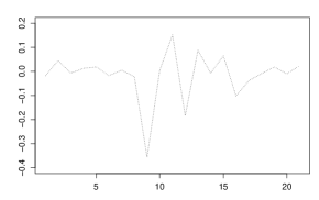
(a) Residuals versus iterations

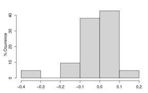
(b) Residual histogram

Figure 2: Pearson residuals – Seed germination

5.1 Chain convergence in the tilted beta binomial model

In the parameter estimation process, three posterior samples were generated beginning from different starting values. In all chains, the autocorrelation is close to zero for a lag greater than or equal than 10, and a burn-in bigger than 10000.

To check the convergence of the chains, two convergence diagnoses were applied: the Geweke diagnostic (Geweke,, 1992) and the Brooks-Gelman-Rubin convergence diagnostic (Brooks and Gelman,, 1998). The Geweke-Brooks plot for the chains of the regression parameters can be observed in Figure 3, where the value of the $Z$ statistic versus the number of iterations is plotted to determine the burn-in of the chains. This figure shows that the statistic remains within the acceptance zone for a period of burn-in equal to zero. The second method applied is known as the Brooks-Gelman and Rubin convergence diagnostic. It was proposed by Brooks and Gelman, (1998) and compares within-chain and between-chain variances through the estimation of the statistic of scale reduction $R$. Values of $R$ well above 1 indicate that the chains have not converged. Figure 4 shows that for the regression parameters of this example, the R factor is very close to 1 after the 1000 iterations.

Figure 3: Geweke convergence diagnostic - Seed germination

Figure 4: Brooks-Gelman and Rubin convergence diagnostic - Seeds germination

5.2 Models comparison

In order to determine the performance of the proposed model, the following models also were fitted to the seed germination dataset: binomial $Bin(n,p$), beta binomial $BB(\mu,\phi$) and beta rectangular binomial $BRB(\mu,\phi,\theta$). The deviance and the deviance information Criterion (DIC) for each of these models are given in Table 2, which shows that the lowest average of the deviance and the lowest DIC value correspond to the tilted beta binomial and the beta rectangular binomial models, where the first one presents the lowest DIC value and therefore is the best model.

Model	DIC	Deviance
		Mean	S.D.	Cred. Interval 95%	Median
Bin($n$,$p$)	174.6	172.8	1.827	(172.8,179.5)	174.1
BB($mu$,$\phi$)	154.6	149.3	2.87	(145.8,156.6)	148.6
BRB($\mu,\phi,\theta$)	123.4	116.9	3.59	(112.2,125.7)	116.3
TBB($\mu_{t},\mu_{b},\phi,\theta$)	121.9	116.7	3.54	(112.1,125.2)	116

Table 2: Statistics for model comparison - Seed germination

6 Conclusion

In this paper two new distributions are proposed: the tilted beta binomial distribution and the beta rectangular binomial distribution. From these distributions, assuming that their parameters follow regression structures, new overdispersion regression models for count data are proposed: the tilted beta binomial regression model and the beta rectangular binomial regression model. These models are fitted using Bayesian methods, and in the application, show better performance than the beta binomial regression models for statistical analysis of the seed germination dataset.

Given that the tilted beta distribution is flexible and allows considering varying amounts with greater likelihoods than the beta distribution in the extreme tail-area events, it permits accommodating different relative likelihoods of high versus low extreme tail-area events. Thus, the proposed tilted beta binomial regression model which defines a more general overdispersion regression model than the beta binomial regression model, allows considering count events with high or low likelihood of occurrence and better estimation of the regression parameters, credibility (or confidence) intervals and statistical inferences in the analysis of binomial-type overdispersion data.

Appendix A OpenBUGS code for the TBB regression model

⬇

model{

#Likelihood:

for( i in 1 : N ){

zeros[i]<-0

zeros[i]~dloglik(loglike[i])

loglike[i]<-log(theta[i]*fd_b[i]+(1-theta[i])*fd_BB[i])

#fd_b: beta function part

#fd_BB: loglikelihood for beta binomial part

fd_b[i]<-exp(log(2)+logfact(n[i])-logfact(n[i]-y[i])-logfact(y[i])

+loggam(y[i]+1)+loggam(n[i]-y[i]+1)-loggam(y[i]+1+n[i]-y[i]+1)

+log(y[i]*(6*mu_c-3)+n[i]*(2-3*mu_c)+1)-log(n[i]+2))

fd_BB[i]<-exp(logfact(n[i])-logfact(n[i]-y[i])-logfact(y[i])

+loggam(phi[i])+ loggam(y[i]+mu[i]*phi[i])+loggam(n[i]-y[i]

+phi[i]*(1-mu[i])))-loggam(mu[i]*phi[i])

-loggam(phi[i]*(1-mu[i]))-loggam(n[i]+phi[i]))

log(phi[i])<-a[1]+a[2]*(x1[i]+1)

mu[i]<-max(1.0E-6,mu2[i])

logit(mu2[i])<-c[1]+c[2]*(x1[i]+1)

logit(theta[i])<-b[1]+b[2]*(x2[i]+1)

}

#Priors:

mu_t~dunif(0.333333,0.666666)

for (i in 1:2){ a[i] ~ dnorm(0,0.1)}

for (i in 1:2){ b[i] ~ dnorm(0,0.1)}

for (i in 1:2){ c[i] ~ dnorm(0,0.1)}

}

References

- Brooks and Gelman, (1998) Brooks, S. and Gelman, A. (1998). General methods for monitoring convergence of iterative simulations. J. Comput. Graphi. Stat., 7:434–455.
- Cepeda and Gamerman, (2005) Cepeda, E. and Gamerman, D. (2005). Bayesian methodology for modeling parameters in the two parameter exponential family. Revista Estadistica, 57(168-169):93–105.
-
Cepeda-Cuervo, (2001)
Cepeda-Cuervo, E. (2001).
Variability Modeling in Generalized Linear Models.
Unpublished Ph.D. thesis, Mathematics Institute, Universidade Federal
do Rio de Janeiro.
URL: http://www.docentes.unal.edu.co/ecepedac/docs/TESISFINAL.pdf. - Cepeda-Cuervo and Cifuentes-Amado, (2017) Cepeda-Cuervo, E. and Cifuentes-Amado, M. V. (2017). Double generalized beta-binomial and negative binomial regression models. Revista Colombiana de Estadística, 40:141.
- Cepeda-Cuervo and Garrido, (2015) Cepeda-Cuervo, E. and Garrido, L. (2015). Bayesian beta regression models with joint mean and dispersion modeling. Monte Carlo Methods and Applications, 21(1):49–58.
- Collet, (1991) Collet, D. (1991). Modeling Binary Data. Chapman Hall, London.
- Cox, (1983) Cox, D. (1983). Some remarks on overdispersion. Biometrika, 70(1):269–274.
- Crowder, (1978) Crowder, M. J. (1978). Beta-binomial anova for proportions. Applied Statistics, 27:34.
- Efron, (1986) Efron, B. (1986). Double exponential families and their use in generalized linear regression. J.Amer. Statist. Assoc., 81(395):709–721.
- Flegal, (2008) Flegal, J. M. (2008). Monte Carlo standard errors for Markov chain Monte Carlo. Doctoral dissertation, University of MinnesotaMajor: Statistics.
- Geweke, (1992) Geweke, J. (1992). Evaluating the accuracy of sampling-based approaches to calculating posterior moments. In Bernardo, J. M., Berger, J., Dawid, A. P., and Smith, J. F. M., editors, Bayesian Statistics 4, pages 169–193. Oxford University Press, Oxford.
- Hahn, (2008) Hahn, E. (2008). Mixture densities for project management activity times: A robust approach to pert. European Journal of Operational Research, 188:450–459.
- Hahn and López Martín, (2015) Hahn, E. and López Martín, M. (2015). Robust project management with the tilted beta distribution. SORT, 39:253–272.
- Hinde and Demétrio, (1998) Hinde, J. and Demétrio, C. (1998). Overdispersion: Models and estimation. Computational Statistics & Data Analysis, 27:151–170.
- Jorgensen, (1997) Jorgensen, B. (1997). Proper dispersion models. Brazilian Journal of Probability and Statistics, 11(2):89–128.
- Spiegelhalter et al., (2003) Spiegelhalter, D., Thomas, A., Best, N., and Lunn, D. (2003). WinBUGS user manual. MRC Biostatistics Unit, Institute of Public Health, Cambridge, UK.
- Williams, (1982) Williams, D. (1982). Extra-binomial variation in logistic linear models. Appl.Statist., 2:144–188.