SUSY threshold corrections to quark and lepton mixing
inspired by $SO(10)$ GUT models

Abstract

In the standard model (SM), the Cabibbo-Kobayashi-Maskawa (CKM) matrix is the only origin of flavor violations (FVs). On the other hand, in general, there are a lot of sources of the FVs in a physics beyond the SM, through the diagonalizing matrices which make Yukawa matrices diagonal. Although most of the diagonalizing matrices are unknown ones, grand unified theories (GUTs) can fix these matrices. In particular, if we consider a GUT model based on the $SO(10)$ group, these diagonalizing matrices are strongly related to each other because of the matter unification. However, this unification causes the problem on the realization of measured SM fermion masses and mixing angles. Up to now, many people showed that supersymmetric (SUSY) threshold corrections can solve this problem, especially unfavorable fermion mass relations. In this paper, we show that how these SUSY threshold corrections affect unknown diagonalizing matrices. Since these contributions are also related to the FVs induced by SUSY particles, we can estimate the maximal effect to the diagonalizing matrices. We found that the $(1,3)$ and $(3,1)$ elements of diagonalizing matrices for quarks can be as large as the corresponding mixing angle of the CKM matrix. Moreover, we found that the higher SUSY scale can predict the larger mixing angles, although strong cancellation between the Higgs mass parameters is needed to realize the electroweak symmetry breaking.

1 Introduction

Observing Higgs boson [1] establishes the standard model (SM) completely. However, some topics such as non-zero neutrino masses and existence of the dark matter are not explained in the SM, and then, many physics beyond the SM (bSMs) are established to explain these topics. So far, many experiments have tried to find the signals of the new physics and they reported the results about upper and/or lower limits or observed values for some observables. We can now test the bSMs by using these limits and observables.

One of the most important tools to test the bSMs is flavor phenomena. Flavor observables can probe effects of new particles with masses far above the energy scale of current collider experiments. In the SM, the only origin of flavor violations (FVs) is the Cabibbo-Kobayashi-Maskawa (CKM) matrix [2] which is defined by a product of the mixing matrices of left-handed quarks. Small mixing angles of the CKM matrix cause small FVs for the SM predictions, and therefore, flavor observables show us clear signal of the bSMs.

In general, there are additional origins of the FVs in the bSMs. Especially, the diagonalizing matrices play a crucial role among these origins. Well-known examples are supersymmetric (SUSY) models. In these models, FVs can be induced by mediating the SUSY particles. To predict flavor observables via contributions from SUSY particles, mass insertion parameters (MIPs) in a super-CKM basis [3] are often used. The super-CKM basis is a basis in which the rotations for obtaining diagonal Yukawa matrices are applied to sfermions as well as the SM fermions. Because of this rotation, MIPs include information of the corresponding diagonalizing matrices. However, most of the diagonalizing matrices are unknown ones because what we know about these matrices from the experiments is only the CKM matrix .

One of the possibilities to know the information of these unknown diagonalizing matrices is considering the model with grand unifications. In grand unified theories (GUTs), the three gauge interactions in the SM are unified into a single one, and moreover, the particles in the SM are unified into fewer multiplets [4]. The latter unification reduces degrees of freedom of the diagonalizing matrices. In the GUTs, new particles are predicted, and they also induce FVs through unknown diagonalizing matrices. Although these contributions are negligible for most processes because new particles which induce FVs have masses around the GUT scale, proton decays have a sensitivity for these contributions. Recently, the Super-Kamiokande Collaboration reported some events which can be candidates for proton decay, and these include a candidate for FV decay of the proton such as $p\to\pi\mu$ decay mode [5]. It has been confirmed that in some models, this FV decay of the proton can be comparable to main decay mode of the proton [6].

In the minimal $SO(10)$ GUT models [7] , all quarks and leptons are unified into only one multiplet ${\bf 16}$ for one family. Because of this unification, all diagonalizing matrices become the CKM-like matrix to realize the CKM matrix except for a light neutrino mixing matrix. Note that the mixing angles of the light neutrino mixing matrix can be large because of new degrees of freedom from seesaw mechanism [8, 9]. However because of the unification, it is not easy to realize measured quark and lepton masses and mixings. One useful correction to solve this problem is a SUSY threshold correction [3, 10].

These SUSY threshold corrections mainly come from the soft SUSY-breaking trilinear couplings $A_{\psi}$ (A-terms) and the Higgsino mass parameter $\mu$, and are especially used to realize measured quark and lepton masses [11]. It is known that off-diagonal parts of the A-terms contribute to the CKM matrix [12]. This means that the SUSY threshold corrections also contribute to the diagonalizing matrices. Therefore, it is important to estimate the contributions from the SUSY threshold correction to the diagonalizing matrices.

In this paper, we discuss how large diagonalizing matrices originated from the SUSY threshold corrections are allowed in the minimal SUSY $SO(10)$ GUT model. In this setup, we may obtain some specific signal for the model from the effect of large diagonalizing matrices. Note that large off-diagonal parts of fermion mass matrices which generate large diagonalizing matrices come from large off-diagonal parts of the A-terms through the SUSY threshold corrections. However, these off-diagonal parts are strongly constrained by flavor phenomena like SUSY flavor-changing neutral currents (FCNCs) . Furthermore, these also cause the negative mass squared for sfermions through the renormalization group equation (RGE) effects. Then, we calculate the maximal size of diagonalizing matrices numerically without conflicting with these concerns.

This paper is organized as follow. In Sec. 2, we show the notation used in this paper. We give the method of our calculation in Sec. 3, and our main results are shown in Sec. 4. The conclusion is in Sec. 5. In addition, we show the detail of the SUSY threshold corrections in Appendix A. We also summarize the relevant constraints to our calculation in Appendix B. The discussion about the maximal SUSY threshold correction which satisfy the constraints are shown in Appendix C.

2 Notation

In this section, we summarize our notation in this paper. The superpotential for the Yukawa interactions and $\mu$ term in the interaction basis is

$$W=\epsilon_{ab}\left[(Y_{u})_{ij}Q_{L\,i}^{a}U_{R\,j}^{c}H_{u}^{b}-(Y_{d})_{ij}Q_{L\,i}^{a}D_{R\,j}^{c}H_{d}^{b}-(Y_{e})_{ij}L_{L\,i}^{a}E_{R\,j}^{c}H_{d}^{b}\right]+\epsilon_{ab}\mu H_{u}^{a}H_{d}^{b},$$ (1)

where $Q_{L}$, $L_{L}$, $U_{R}^{c}$, $D_{R}^{c}$, $E_{R}^{c}$, $H_{u}$, and $H_{d}$ are superfields of the left-handed quark doublet, left-handed lepton doublet, right-handed up-type quark, right-handed down-type quark, right-handed charged-lepton, up-type Higgs doublet, and down-type Higgs doublet, respectively. In this paper, we use the capital letters for superfields and the small letters for the corresponding SM components. Here, $Y_{u}$, $Y_{d}$, and $Y_{e}$ are the up-type quark, down-type quark, and charged lepton Yukawa matrices, $a$, $b=1,\,2$ are weak isospin indices, $i$, $j=1,\,2,\,3$ are generation indices, and $\epsilon_{12}\equiv+1$ is an antisymmetric tensor. To obtain fermion masses, neutral components of CP-even Higgses develop vacuum expectation values (VEVs) $\langle h^{0}_{u(d)}\rangle\equiv v_{u(d)}$ whose ratio is defined as $\tan\beta\equiv v_{u}/v_{d}$. The mass basis of fermions are obtained by diagonalizing Yukawa matrices as

$$\psi_{L\,i}(Y_{\psi})_{ij}\psi_{R\,j}^{c}=(L_{\psi}^{\dagger}\psi_{L})_{i}(L_{\psi}^{T}Y_{\psi}R_{\psi})_{ij}(R_{\psi}^{\dagger}\psi_{R}^{c})_{j}=(\hat{Y}_{\psi})_{ii}\psi^{\prime}_{L\,i}\psi^{\prime}{}_{R\,i}^{c},$$ (2)

where $\psi$ and $\psi^{\prime}$ indicate the SM fermion in the interaction basis and mass basis, $L_{\psi}$ and $R_{\psi}$ are diagonalizing matrices for the left-handed and right-handed fermion, and $(\hat{Y}_{\psi})_{ii}$ is the Yukawa coupling of $i$-th generation fermion $\psi$. The same rotations are applied to the corresponding sfermions because of the SUSY, and this basis is called the super-CKM basis. In this paper, $\hat{X}$ refers to the parameter of $X$ in the super-CKM basis. We calculate mixing angles for the diagonalizing matrices, defined as

$$L_{\psi}^{T} \equiv\begin{pmatrix}c_{12}^{\psi L}&-s_{12}^{\psi L}&0\\ s_{12}^{\psi L*}&c_{12}^{\psi L}&0\\ 0&0&1\end{pmatrix}\begin{pmatrix}c_{13}^{\psi L}&0&-s_{13}^{\psi L}\\ 0&1&0\\ s_{13}^{\psi L*}&0&c_{13}^{\psi L}\end{pmatrix}\begin{pmatrix}1&0&0\\ 0&c_{23}^{\psi L}&-s_{23}^{\psi L}\\ 0&s_{23}^{\psi L*}&c_{23}^{\psi L}\end{pmatrix},$$ (3)

$$R_{\psi} \equiv\begin{pmatrix}1&0&0\\ 0&c_{23}^{\psi R}&s_{23}^{\psi R}\\ 0&-s_{23}^{\psi R*}&c_{23}^{\psi R}\end{pmatrix}\begin{pmatrix}c_{13}^{\psi R}&0&s_{13}^{\psi R}\\ 0&1&0\\ -s_{13}^{\psi R*}&0&c_{13}^{\psi R}\end{pmatrix}\begin{pmatrix}c_{12}^{\psi R}&s_{12}^{\psi R}&0\\ -s_{12}^{\psi R*}&c_{12}^{\psi R}&0\\ 0&0&1\end{pmatrix},$$ (4)

where $s_{ij}^{\psi L/R}\equiv\sin\theta_{ij}^{\psi L/R}e^{-i\chi_{ij}^{\psi L/R}}$, and $c_{ij}^{\psi L/R}\equiv\cos\theta_{ij}^{\psi L/R}$ .

To calculate the SUSY threshold corrections, we use following soft-breaking parameters in a Lagrangian $\mathcal{L}_{\text{soft}}$,

$$\mathcal{L}_{\text{soft}} = -\frac{1}{2}\left(M_{1}\tilde{b}\tilde{b}+M_{2}\tilde{w}\tilde{w}+M_{3}\tilde{g}\tilde{g}\right)-\epsilon_{ab}B_{\mu}h_{u}^{a}h_{d}^{a}+h.c.$$ (5)

$$-\epsilon_{ab}\left[(A_{u})_{ij}\tilde{q}_{L\,i}^{a}\tilde{u}^{*}_{R\,j}h_{u}^{b}-(A_{d})_{ij}\tilde{q}_{L\,i}^{a}\tilde{d}^{*}_{R\,j}h_{d}^{b}-(A_{e})_{ij}\tilde{l}_{L\,i}^{a}\tilde{e}^{*}_{R\,j}h_{d}^{b}\right]+h.c.$$

$$-m_{h_{u}}^{2}h_{u}^{\dagger}h_{u}-m_{h_{d}}^{2}h_{d}^{\dagger}h_{d}-(m_{\tilde{q}}^{2})_{ij}\tilde{q}^{\dagger}_{L\,i}\tilde{q}_{L\,j}-(m_{\tilde{l}}^{2})_{ij}\tilde{l}^{\dagger}_{L\,i}\tilde{l}_{L\,j}$$

$$-(m_{\tilde{u}}^{2})_{ij}\tilde{u}^{*}_{R\,i}\tilde{u}_{R\,j}-(m_{\tilde{d}}^{2})_{ij}\tilde{d}^{*}_{R\,i}\tilde{d}_{R\,j}-(m_{\tilde{e}}^{2})_{ij}\tilde{e}^{*}_{R\,i}\tilde{e}_{R\,j}$$

where $M_{i}$ ($i=1,2,3$) are gaugino masses, and $\tilde{\psi}$ is the SUSY partner for the corresponding SM particle $\psi$. Moreover, we define following 6$\times$6 sfermion mass squared matrices as

$$\mathcal{L}_{\text{mass}}=-\hat{M}_{\tilde{\psi}\,ij}^{2}\tilde{\psi}_{i}^{\dagger}\tilde{\psi}_{j},\quad\tilde{\psi}=\begin{pmatrix}\tilde{\psi}_{L\,1}&\tilde{\psi}_{L\,2}&\tilde{\psi}_{L\,3}&\tilde{\psi}_{R\,1}&\tilde{\psi}_{R\,2}&\tilde{\psi}_{R\,3}\end{pmatrix}^{T},$$ (6)

where

$$\hat{M}_{\tilde{u}}^{2}=\begin{pmatrix}\hat{m}^{2}_{\tilde{q}}+v_{u}^{2}\hat{Y}_{u}\hat{Y}_{u}&v_{u}\hat{A}_{u}^{*}-\mu v_{d}\hat{Y}_{u}\\ v_{u}\hat{A}_{u}^{T}-\mu^{*}v_{d}\hat{Y}_{u}&\hat{m}^{2}_{\tilde{u}}+v_{u}^{2}\hat{Y}_{u}\hat{Y}_{u}\end{pmatrix}\equiv\begin{pmatrix}\Delta_{LL}^{u}&\Delta_{LR}^{u}\\ \Delta_{RL}^{u}&\Delta_{RR}^{u}\end{pmatrix},$$ (7)

$$\hat{M}_{\tilde{d}}^{2}=\begin{pmatrix}V_{\text{CKM}}^{\dagger}\hat{m}^{2}_{\tilde{q}}V_{\text{CKM}}+v_{d}^{2}\hat{Y}_{d}\hat{Y}_{d}&v_{d}\hat{A}_{d}^{*}-\mu v_{u}\hat{Y}_{d}\\ v_{d}\hat{A}_{d}^{T}-\mu^{*}v_{u}\hat{Y}_{d}&\hat{m}^{2}_{\tilde{d}}+v_{d}^{2}\hat{Y}_{d}\hat{Y}_{d}\end{pmatrix}\equiv\begin{pmatrix}\Delta_{LL}^{d}&\Delta_{LR}^{d}\\ \Delta_{RL}^{d}&\Delta_{RR}^{d}\end{pmatrix},$$ (8)

$$\hat{M}_{\tilde{e}}^{2}=\begin{pmatrix}\hat{m}^{2}_{\tilde{l}}+v_{d}^{2}\hat{Y}_{e}\hat{Y}_{e}&v_{d}\hat{A}_{e}^{*}-\mu v_{u}\hat{Y}_{e}\\ v_{d}\hat{A}_{e}^{T}-\mu^{*}v_{u}\hat{Y}_{e}&\hat{m}^{2}_{\tilde{e}}+v_{d}^{2}\hat{Y}_{e}\hat{Y}_{e}\end{pmatrix}\equiv\begin{pmatrix}\Delta_{LL}^{e}&\Delta_{LR}^{e}\\ \Delta_{RL}^{e}&\Delta_{RR}^{e}\end{pmatrix}.$$ (9)

The sfermion mass squared matrix $\hat{M}_{\tilde{\psi}\,ij}^{2}$ is diagonalized by a unitary matrix $U_{\tilde{\psi}}$ as

$$\hat{M}_{\tilde{\psi},\text{diag}}^{2}=U_{\tilde{\psi}}\hat{M}_{\tilde{\psi}}^{2}U_{\tilde{\psi}}^{\dagger}.$$ (10)

The SUSY threshold corrections are induced by chirality-flipping self-energies. In Ref. [14], the details of the calculation for these corrections are shown in a decoupling limit $M_{\text{SUSY}}\gg v$ where $M_{\text{SUSY}}$ and $v$ are the SUSY scale and the VEV of the SM Higgs. We also apply to this decoupling limit in this paper. In the Appendix A, we summarize the SUSY threshold corrections in our notation.

The SUSY threshold corrections affect on the diagonalizing matrices if chirality-flipping self-energies have off-diagonal parts which come from the off-diagonal parts of A-terms and sfermion mass squared matrices. The size of these off-diagonal parts are important to obtain the large SUSY threshold corrections. However, these off-diagonal parts are also related to the SUSY FCNCs, and therefore, these sizes are constrained from the experimental measurements. Moreover, large off-diagonal parts of A-terms make the sfermion squared mass negative and cause the a charge and color breaking (CCB) [15]. In the Appendix B, we summarize the SUSY FCNC and CCB constraints, used in this paper.

3 Method of the calculation

From the following, we explain the calculation of the diagonalizing matrices with the SUSY threshold corrections. To calculate the diagonalizing matrices, we have to set the input parameters at the GUT scale. In our model, these parameters are the unified gauge coupling $g_{\text{GUT}}$, unified Yukawa matrix $Y_{\text{GUT}}$, unified gaugino mass $M_{1/2}$, the scale of A-terms $A_{0}$, universal sfermion mass $m_{16}^{2}$, Higgs mass parameter $m_{10}^{2}$, and Higgs mass difference $\Delta m_{h}^{2}$ which is needed to realize the electroweak symmetry breaking (EWSB). Note that for simplicity and for reducing the parameters, we assume $\Delta m_{h}^{2}\sim M_{\rm SUSY}^{2}$. We discuss the Yukawa unification at the beginning since we can fix part of the input parameters from it.

3.1 SUSY threshold correction for realizing Yukawa unification

The SUSY threshold correction plays an important role for realizing the Yukawa unification in the SUSY $SO(10)$ GUT models. When we consider this Yukawa unification, we can fix the unified gauge coupling $g_{\text{GUT}}$ and (3,3) component of unified Yukawa matrix $(Y_{\text{GUT}})_{33}$. The latter one is obtained by setting the values of the SUSY threshold corrections and $\tan\beta$ appropriately. Note that some of the other parameters can be fixed by the other assumptions, as we explain later.

First of all, we find the required SUSY threshold correction and $\tan\beta$ for realizing the Yukawa unification. In this calculation, we start from the central values of the experimental measurements summarized in Table 1.

$m_{s}/((m_{u}+m_{d})/2)$	$27.3^{+0.7}_{-1.3}$	$m_{e}$	$0.5109989461(31)$ MeV
$m_{d}$	$4.67^{+0.48}_{-0.17}$ MeV	$m_{\mu}$	$105.6583745(24)$ MeV
$m_{s}$	$93^{+11}_{-5}$ MeV	$m_{\tau}$	1776.86$\pm 0.12$ MeV
$m_{c}$	$1.27\pm 0.02$ GeV	$M_{Z}$	91.1876(21) GeV
$m_{b}(m_{b})$	4.180${}^{+0.04}_{-0.03}$ GeV	$M_{W}$	$80.379(12)$ GeV
$m_{t}$(direct detection)	173.0$\pm 0.4$ GeV	$G_{F}$	1.1663787(6)$\times 10^{-5}$ GeV-2
$\sin^{2}\theta_{W}$	0.23122(4)	$\alpha_{s}(M_{Z})$	$0.1181(11)$
$\alpha$	1/137.036

Table 1: The input parameters in our analysis. All values come from Ref. [17].

There are three scales which are relevant to our calculation: $M_{Z}$, $M_{\rm SUSY}$, and the GUT scale $M_{\rm GUT}$. First, we calculate the parameters at the $M_{Z}$ scale from the input parameters in Table 1. For calculating the running quark masses, we use the Mathematica package RunDec [18], while for the running lepton masses, we translate the lepton pole masses to running masses at the $M_{Z}$ scale, following Ref. [19]. Next, we derive the couplings at the SUSY scale from those at the $M_{Z}$ scale, using the SM RGE at the two-loop level [20, 21] . At the SUSY scale, we translate the $\overline{\text{MS}}$ scheme into the $\overline{\text{DR}}$ scheme according to Ref. [25]. After applying the matching condition by using the $\tan\beta$, we add the SUSY threshold corrections as

$$y_{t}(M_{\text{SUSY}}) = \frac{1}{\sin\beta}y^{(0)}_{t}(M_{\text{SUSY}})+\Delta y_{t}(M_{\text{SUSY}}),$$

$$y_{b}(M_{\text{SUSY}}) = \frac{1}{\cos\beta}y^{(0)}_{b}(M_{\text{SUSY}})+\Delta y_{b}(M_{\text{SUSY}}),$$ (11)

$$y_{\tau}(M_{\text{SUSY}}) = \frac{1}{\cos\beta}y^{(0)}_{\tau}(M_{\text{SUSY}})+\Delta y_{\tau}(M_{\text{SUSY}}),$$

where $\Delta y_{\psi}$ shows the SUSY threshold correction for the fermion $\psi$. However in this section, we only consider $\Delta y_{b}$ because this contribution is dominant over the other ones. Here ⁽⁰⁾ means parameters below the SUSY scale, namely, SM parameters. Finally, we derive the couplings at the GUT scale from those at the SUSY scale, using the minimal SUSY SM (MSSM) RGE at the two-loop level [26]. Note that in our calculation, $M_{\rm GUT}$ and $g_{\rm GUT}$ are defined as

$$g_{1}(M_{\text{GUT}})=g_{2}(M_{\text{GUT}})\equiv g_{\text{GUT}},$$ (12)

where $g_{1}$ is the GUT normalized gauge coupling for the $U(1)_{Y}$, and $g_{2}$ is the gauge coupling for the $SU(2)_{L}$. By means of this procedure, we can obtain the required value of $\Delta y_{b}$ and $\tan\beta$ for realizing the Yukawa unification: $y_{t}=y_{b}=y_{\tau}$.

In Fig. 1, we show the dependence of $\Delta y_{b}$ and $\tan\beta$ on $M_{\text{SUSY}}$.

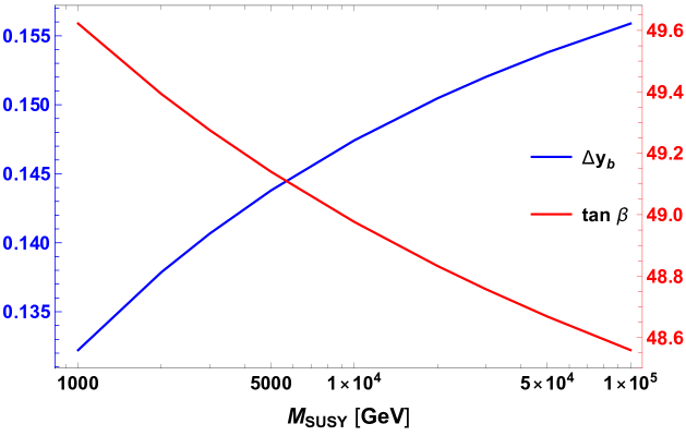
Figure 1: Dependence of the required SUSY threshold correction $\Delta y_{b}$ and $\tan\beta$ for realizing the $SO(10)$ Yukawa unification on $M_{\text{SUSY}}$. The blue line and axis show the result for the required SUSY threshold correction, and the red ones show the result for the $\tan\beta$.

The blue line and axis show the required SUSY threshold correction, and the red ones show the $\tan\beta$. From this figure, importance of large $\tan\beta$ is clear which has been already discussed in Ref. [27]. Interestingly, it is shown that a maximal SUSY threshold correction is larger than the required one because of the large $\mu$ contribution when the SUSY scale is below 100 TeV. In Appendix C, we discuss this issue by considering the CCB and EWSB constraints. Note that the SUSY threshold correction for the diagonal part is dominated by the contributions from $\mu$ parameter in the case of large $\tan\beta$. Therefore in this paper, the $\mu$ parameter is fixed to realize the required SUSY threshold correction, and we use a maximal A-term to maximize the effect to the diagonalizing matrices.

3.2 SUSY threshold correction for the diagonalizing matrices

In this section, we explain how to calculate the SUSY threshold correction for the diagonalizing matrices. In this calculation, we use the eigenvalues of Yukawa matrices at the GUT scale. Therefore, when the SUSY threshold corrections are absent, the Yukawa matrices are diagonal matrices at any energy scales, and hence, the corresponding diagonalizing matrices are unit matrices. There are some advantages in this setup. First one is that contributions from the SUSY threshold corrections to the diagonalizing matrices become clear. Origins of the SUSY threshold corrections to the diagonalizing matrices are off-diagonal parts of SUSY parameters $A_{\psi}$ and $m_{\tilde{\psi}}^{2}$ in the super-CKM basis. If the Yukawa matrices have the off-diagonal elements, these parts become the combination of those in the interaction basis and the diagonalizing matrices, which leads to the contributions are unclear. The second advantage is that we can exclude some unfavorable contributions to the SUSY threshold corrections. In many cases, family symmetries which show us how to realize the CKM matrix are introduced with the $SO(10)$ symmetry. However for this calculation, these family symmetries are unfavorable because these affect and fix the diagonalizing matrices. By using diagonal Yukawa matrices, we can remove these unfavorable contributions.

In our calculation, we use the following assumptions at the GUT scale:

$$M_{1}=M_{2}=M_{3}=M_{1/2},$$ (13)

$$A_{u}=A_{0}\hat{Y_{u}}+\delta A,~{}~{}A_{d}=A_{0}\hat{Y_{d}}+\delta A,~{}~{}A_{e}=A_{0}\hat{Y_{e}}+\delta A,$$

$$m_{\tilde{q}}^{2}=m_{\tilde{l}}^{2}=m_{\tilde{u}}^{2}=m_{\tilde{d}}^{2}=m_{\tilde{e}}^{2}=m_{16}^{2}\,1_{3\times 3},$$ (14)

$$m_{h_{u}}^{2}=m_{10}^{2}-\Delta m_{h}^{2},~{}~{}m_{h_{d}}^{2}=m_{10}^{2}+\Delta m_{h}^{2},$$

where $\delta A$ indicates the off-diagonal part of the A-terms. Note that if $\delta A=0$, each diagonalizing matrix becomes the unit matrix. Since we set $\Delta m_{h}^{2}\sim M_{\rm SUSY}^{2}$, there are 5 parameters in this setup, $M_{1/2}$, $A_{0}$, $\delta A$, $m_{16}$, and $m_{10}$. In order to reduce the parameters, we take the following assumptions: (i) the gluino mass at the SUSY scale is around $M_{\rm SUSY}$; (ii) the SUSY scale is defined by two stop masses as $M_{\rm SUSY}=\sqrt{m_{\tilde{t}_{L}}(M_{\text{SUSY}})m_{\tilde{t}_{R}}(M_{\text{SUSY}})}$. Therefore, once we fix $A_{0}$, $\delta A$, and $m_{10}$ in each $M_{\rm SUSY}$ case, we can determine $M_{1/2}$ and $m_{16}$ by (i) and (ii), respectively. The remaining parameters can be determined so that the SUSY FCNC and CCB constraints are satisfied and the required SUSY threshold correction are obtained. Note that we also check whether the EWSB can be realized. Among such parameter sets, we take the set which maximizes the A-terms and calculate the diagonalizing matrices.

After we calculate the diagonalizing matrices, we extract mixing angles by following Eqs. (3) and (4). Moreover we compare these mixing angles and those of the measured CKM matrices [17], which are

$$s_{12}^{\text{CKM}}=2.2496\times 10^{-1},\,s_{23}^{\text{CKM}}=4.16\times 10^{-2},\,s_{13}^{\text{CKM}}=4.09\times 10^{-3},$$ (15)

where the CKM matrix $V_{\text{CKM}}$ is defined as

$$V_{\text{CKM}}\equiv\begin{pmatrix}1&0&0\\ 0&c_{23}^{\text{CKM}}&s_{23}^{\text{CKM}}\\ 0&-s_{23}^{\text{CKM}*}&c_{23}^{\text{CKM}}\end{pmatrix}\begin{pmatrix}c_{13}^{\text{CKM}}&0&s_{13}^{\text{CKM}}\\ 0&1&0\\ -s_{13}^{\text{CKM}*}&0&c_{13}^{\text{CKM}}\end{pmatrix}\begin{pmatrix}c_{12}^{\text{CKM}}&s_{12}^{\text{CKM}}&0\\ -s_{12}^{\text{CKM}*}&c_{12}^{\text{CKM}}&0\\ 0&0&1\end{pmatrix}.$$ (16)

If the diagonalizing matrices are as large as or larger than the CKM matrix, the SUSY threshold corrections affect on the CKM matrix. In that case, the CKM matrix is obtained by the combination of the diagonalizing matrices from the SUSY threshold corrections and Yukawa matrices, or some cancellations are needed between the diagonalizing matrices to realize the CKM matrix.

Since $s_{13}^{\rm CKM}$ is smaller than the other elements, we calculate $s_{13}^{\psi L,R}$ by setting $\delta A$ as

$$\delta A=\begin{pmatrix}0&0&A_{\rm off}\\ 0&0&0\\ A_{\rm off}&0&0\end{pmatrix}.$$ (17)

In this case, we should take care about the SUSY FCNCs, especially $B_{d}$-$\overline{B_{d}}$ mixing and $\tau\to e\gamma$. The details of calculations and constraints for these processes are summarized in the Appendix B. In the other case of $\delta A$, the contributions to the corresponding diagonalizing matrices are expected to be small due to the largeness of $s_{ij}^{\rm CKM}$ and/or the SUSY FCNC constraints.

4 Results

The input parameters which satisfies the constraints and realizes the required SUSY threshold correction simultaneously are shown in Table 2.

	$M_{\rm SUSY}$ = 2 TeV	$M_{\rm SUSY}$ = 10 TeV	$M_{\rm SUSY}$ = 100 TeV
$M_{\rm GUT}$	$1.2\times 10^{16}$ GeV	$7.4\times 10^{15}$ GeV	$3.6\times 10^{15}$ GeV
$g_{1}=g_{2}$	0.70	0.68	0.66
$g_{3}$	0.70	0.69	0.67
$y_{u}$	$3.0\times 10^{-6}$	$3.0\times 10^{-6}$	$3.1\times 10^{-6}$
$y_{c}$	$1.5\times 10^{-3}$	$1.5\times 10^{-3}$	$1.5\times 10^{-3}$
$y_{d}$	$3.4\times 10^{-4}$	$3.4\times 10^{-4}$	$3.4\times 10^{-4}$
$y_{s}$	$6.5\times 10^{-3}$	$6.5\times 10^{-3}$	$6.5\times 10^{-3}$
$y_{e}$	$1.4\times 10^{-4}$	$1.3\times 10^{-4}$	$1.3\times 10^{-4}$
$y_{\mu}$	$2.9\times 10^{-2}$	$2.8\times 10^{-2}$	$2.8\times 10^{-2}$
$y_{t}=y_{b}=y_{\tau}$	0.58	0.56	0.54
$M_{1/2}$	$9.3\times 10^{2}$ GeV	$5.2\times 10^{3}$ GeV	$5.9\times 10^{4}$ GeV
$A_{0}^{\rm max}$	$-5.5\times 10^{3}$ GeV	$-2.4\times 10^{4}$ GeV	$-1.8\times 10^{5}$ GeV
$A_{\rm off}$	$-98$ GeV	$-2.4\times 10^{3}$ GeV	$-1.4\times 10^{5}$ GeV
$m_{16}$	$3.9\times 10^{3}$ GeV	$1.7\times 10^{4}$ GeV	$2.1\times 10^{5}$ GeV
$m_{10}$	$4.9\times 10^{3}$ GeV	$2.0\times 10^{4}$ GeV	$2.9\times 10^{5}$ GeV
$\Delta m_{h}^{2}/M_{\rm SUSY}^{2}$	$1$	$0.48$	$1$

Table 2: The input parameters at the GUT scale. In this table, we show the results of the case where the structure of $\delta A$ is Eq. (17).

Here, $A_{0}^{\rm max}$ is the maximal value of $A_{0}$ which satisfies the CCB constraints. Note that the value of $\Delta m_{h}^{2}$ for $M_{\rm SUSY}=10$ TeV should be smaller than $M_{\rm SUSY}^{2}$. We will explain this issue later. By using these input parameters, we can calculate the mixing angles for $L_{\psi}$ and $R_{\psi}$. We show the results in Table 3.

$M_{\rm SUSY}$	2 TeV	10 TeV	100 TeV
$L_{u}$	$-0.27$	$-1.5$	$-8.2$
$R_{u}$	$-0.25$	$-1.4$	$-7.8$
$L_{d}$	$0.27$	$1.8$	$9.6$
$R_{d}$	$0.54$	$3.6$	$17$
$L_{e}$	$-0.052$	$-0.34$	$-1.2$
$R_{e}$	$-0.12$	$-0.81$	$-2.8$

Table 3: The results of $s_{13}^{\psi L,R}$ in $10^{-3}$ unit for each case of $M_{\rm SUSY}$.

From these results, we found that $s_{13}^{qL,R}$ $(q=u,d)$ can be as large as $s_{13}^{\rm CKM}$ when $M_{\rm SUSY}$ becomes large. This is because the SUSY FCNC constraints become weak in large $M_{\rm SUSY}$ case, and therefore, we can take large $A_{\rm off}$. In this case, however, a strong cancellation between $|m_{h_{u}}^{2}|$ and $m_{h_{d}}^{2}$ is needed to realize the EWSB.

In order to specify that our input parameters realize the maximal size of $s_{13}^{\psi L,R}$ , we show the parameter spaces for $s_{13}^{dL}$ in each $M_{\rm SUSY}$ case in Figs. 2 and 3.

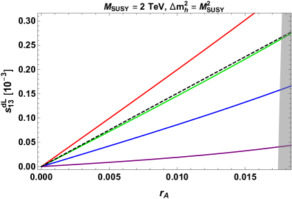
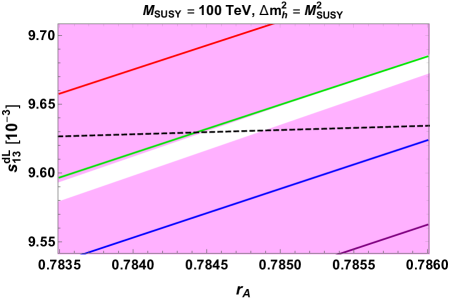
Figure 2: The parameter spaces allowed by the EWSB and SUSY FCNC constraints in $(r_{A},s_{13}^{dL})$ plane. The magenta and gray shaded regions show the EWSB and SUSY FCNC constraints, respectively. The red, green, blue, and purple lines show the examples of prediction with different value of $m_{10}^{2}$, which correspond to $r_{h}=1.6$, $1.605$, $1.61$, and $1.615$ in the left panel and $1.843$, $1.844$, $1.845$, and $1.846$ in the right panel. The black dashed line shows the relation between $s_{13}^{dL}$ and $r_{h}$ in each $r_{A}$, which realizes the required SUSY threshold correction.

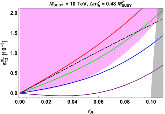
Figure 3: The parameter space allowed by the EWSB and SUSY FCNC constraints in $(r_{A},s_{13}^{dL})$ plane. The color plots show the same meanings as in Fig. 2. In this figure, the red, green, blue, and purple lines correspond to $r_{h}=1.42$, $1.44$, $1.46$, and $1.48$, respectively.

We checked that the situation is same for the other mixing angles. The vertical axis is the mixing angles of $L_{d}$, and the horizontal one is the ratio of $A_{\rm off}$ and $A_{0}^{\rm max}$ at the GUT scale, which is denoted as $r_{A}$. The magenta and gray shaded regions show the EWSB and SUSY FCNC constraints, respectively. The red, green, blue, and purple lines show the examples of prediction with different value of $r_{h}\equiv m_{10}^{2}/m_{16}^{2}$ at the GUT scale. The black dashed line indicates the relation between $s_{13}^{dL}$ and $r_{h}$ in each $r_{A}$, which realizes the required SUSY threshold correction for $y_{b}$. This means that the predicted $\Delta y_{b}$ is larger (smaller) than the required one above (below) the black dashed line. Note that we set $\Delta m_{h}^{2}=M_{\rm SUSY}^{2}$ in Fig. 2, while $\Delta m_{h}^{2}=0.48M_{\rm SUSY}^{2}$ in Fig. 3. This is because $\Delta m_{h}^{2}<M_{\rm SUSY}^{2}$ is needed for the parameter space that satisfies the EWSB and SUSY FCNC constraints and realizes the required SUSY threshold correction simultaneously when $M_{\rm SUSY}=10$ TeV. We found that such parameter space can be obtained when $\Delta m_{h}^{2}\lesssim 0.48M_{\rm SUSY}^{2}$, and then, we set $\Delta m_{h}^{2}=0.48M_{\rm SUSY}^{2}$. On the other hand, we can obtain the parameter space in $M_{\rm SUSY}=2,100$ TeV case even when $\Delta m_{h}^{2}=M_{\rm SUSY}^{2}$ since one of the EWSB and SUSY FCNC constraints is irrelevant in these cases.

From these figures, we can know which constraints determine the maximal value of $s_{13}^{dL}$. For $M_{\rm SUSY}=\mathcal{O}(1)$ TeV case, the SUSY FCNC constraints become the severest one and determine $s_{13}^{dL}$. Note that the EWSB constraints in this case can be satisfied in a wide area of parameter space. In contrast, the SUSY FCNC constraints become weaker and are irrelevant to the significant area for $M_{\rm SUSY}\gtrsim\mathcal{O}(100)$ TeV case. However, the EWSB constraints become severe because of the large values of $|m_{h_{u}}^{2}|$ and $|m_{h_{d}}^{2}|$. This means that a strong cancellation between $|m_{h_{u}}^{2}|$ and $m_{h_{d}}^{2}$ is needed, and therefore, the allowed parameter space is constrained by the EWSB constraints. Interestingly, these constraints determine the size of $s_{13}^{dL}\simeq 9.63\times 10^{-3}$ in our setup when the required SUSY threshold correction is obtained. In the middle $M_{\rm SUSY}$ case, like $M_{\rm SUSY}=10$ TeV, both constraints relate to the maximal value of $s_{13}^{dL}$, as shown in Fig. 3.

It is notable that in our setup, the obtained mixing angles through the SUSY threshold corrections are related with each other due to the $SO(10)$ unification. This means that some of the predictions of FV process can be calculated once one of the predictions of the process are given. Therefore, we may be able to obtain the specific predictions and can test the models by the experiments.

Finally, we comment on the SM fermion masses. Since we do not consider the SUSY threshold corrections for $y_{t}$ and $y_{\tau}$ when we obtain the required SUSY threshold correction for $y_{b}$ and $\tan\beta$, the predictions of $y_{t}$ and $y_{\tau}$ are expected to slightly deviate from the experimental values. We found that the deviation of the top Yukawa coupling is $\mathcal{O}(1)$ % or less, while that of $\tau$ Yukawa coupling is about $3\sim 4$ %. Note that the deviation of bottom Yukawa coupling should be small since we find the parameters for realizing the required SUSY threshold correction. The result for its deviation is less than $0.1$ %, as expected.

5 Conclusion

In this paper, we considered the model with the Yukawa unification inspired by the $SO(10)$ GUT. In this model, we investigated the maximal size of the mixing angles of diagonalizing matrices for the Yukawa matrices, originated from the off-diagonal parts of SUSY threshold corrections. We need large off-diagonal parts of A-terms to obtain the sizable SUSY threshold corrections. However, these parts are constrained by the SUSY FCNC processes. Moreover, the CCB constraints also relate to the maximal value of A-terms. Therefore, we can estimate the maximal contributions to the mixing angles from the SUSY threshold corrections by using these constraints.

We firstly found the required SUSY threshold correction and $\tan\beta$ for realizing the Yukawa unification. As reported in the other papers, the large $\tan\beta\sim 50$ and enough size of $\Delta y_{b}$ are needed. We emphasize that required size of $\Delta y_{b}$ is smaller than the maximal one when $M_{\rm SUSY}\leq 100$ TeV. Therefore, we can obtain required $\Delta y_{b}$ by choosing the input parameters at the GUT scale.

Next, we showed the results for the $s_{13}^{\psi L,R}$ because this element has a possibility to reach the size of corresponding element of the CKM matrix, $s_{13}^{\rm CKM}$. As a result, we found that $s_{13}^{qL,R}$ $(q=u,d)$ can be comparable to $s_{13}^{\rm CKM}$ when $M_{\rm SUSY}>10$ TeV. If the SUSY scale is $\mathcal{O}(1)$ TeV, the off-diagonal parts of A-terms cannot be large because of the SUSY FCNC constraints. Therefore, the results for $s_{13}^{qL,R}$ are about one order of magnitude smaller than $s_{13}^{\rm CKM}$. On the other hand, $M_{\rm SUSY}=100$ TeV case is free from such constraints and predicts large $s_{13}^{qL,R}$, although the EWSB constraints become severe. For $M_{\rm SUSY}=\mathcal{O}(10)$ TeV case, both constraints are relevant to the maximal values of $s_{13}^{qL,R}$, and therefore, we have to find the appropriate value of $\Delta m_{h}^{2}$ to satisfy these constraints.

Importantly, the mixing angles obtained from the SUSY threshold corrections are related with each other when one considers the $SO(10)$ unification as in our setup. Therefore, if one of the FV processes is confirmed, the contributions to the other processes can be calculated, and we can test the models by the (future) experiments. In addition, if some experimental results of the FV process can be explained by these contributions, we may be able to obtain the signature of the $SO(10)$ unification. Furthermore, if the CKM matrix is realized by the other contributions in GUT models, we may find the contribution of the unification according to our results, although it deviates by the RGE effects.

Appendix A SUSY threshold corrections

To calculate the SUSY threshold corrections, chirality-flipping self-energies $\Sigma^{\psi}_{LR}$ are important, which are calculated in Ref. [14] in the decoupling limit $M_{\text{SUSY}}\gg v$. We can divide $\Sigma^{\psi}_{LR}$ for $\psi=u,\,d,\,e$ as

$$\Sigma^{u}_{LR} = \Sigma^{u\tilde{g}}_{LR}+\Sigma^{u\tilde{\chi}^{0}}_{LR},$$ (18)

$$\Sigma^{d}_{LR} = \Sigma^{d\tilde{g}}_{LR}+\Sigma^{d\tilde{\chi}^{0}}_{LR}+\Sigma^{d\tilde{\chi}^{\pm}}_{LR},$$ (19)

$$\Sigma^{e}_{LR} = \Sigma^{e\tilde{\chi}^{0}}_{LR}+\Sigma^{e\tilde{\chi}^{\pm}}_{LR}.$$ (20)

Each part of Eqs. (18), (19), and (20) can be calculated by considering loop contributions from sfermions and fermionic partners of gauge and Higgs bosons. Therefore, we need to diagonalize the sfermion mass squared matrices, shown in Eqs. (7), (8), and (9). For this calculation, we consider the effective Lagrangian within a decoupling limit $M_{SUSY}\gg v$, and hence, we neglect the chirality-flipping elements $\Delta^{\psi}_{LR}$ and $\Delta^{\psi}_{RL}$. Then the diagonalizing matrices for sfermion mass squared matrices, denoted as $U_{\tilde{\psi}}$, can be defined by

$$U_{\tilde{\psi}}\hat{M}_{\tilde{\psi}}^{2}U_{\tilde{\psi}}^{\dagger}=\hat{M}_{\tilde{\psi}\,diag}^{2}={\rm diag}\left(m_{\tilde{\psi}_{L1}}^{2},m_{\tilde{\psi}_{L2}}^{2},m_{\tilde{\psi}_{L3}}^{2},m_{\tilde{\psi}_{R1}}^{2},m_{\tilde{\psi}_{R2}}^{2},m_{\tilde{\psi}_{R3}}^{2}\right),~{}U_{\tilde{\psi}}\equiv\left(\begin{array}[]{cc}U_{\tilde{\psi}}^{L}&0\\ 0&U_{\tilde{\psi}}^{R}\\ \end{array}\right).$$ (21)

For convenience, we introduce

$$(\Lambda_{m}^{\psi\Gamma})_{ij}=(U_{\tilde{\psi}}^{\Gamma\,\dagger})_{im}(U_{\tilde{\psi}}^{\Gamma})_{mj},$$ (22)

where $\Gamma=L,\,R$ is the chirality. We summarize the chirality-flipping self-energies by using these parameters.

The chirality-flipping self-energies from gluino contribution are

$$(\Sigma_{LR\,(mn)}^{d\tilde{g}})_{il} =\frac{2\alpha_{s}}{3\pi}(-M_{3})(\Lambda^{dL}_{m})_{ij}(\Delta^{d}_{LR})_{jk}(\Lambda^{dR}_{n})_{kl}C_{0}(|M_{3}|^{2},\,m_{\tilde{d}_{Lm}}^{2},\,m_{\tilde{d}_{Rn}}^{2}),$$ (23)

$$(\Sigma_{LR\,(mn)}^{u\tilde{g}})_{il} =\frac{2\alpha_{s}}{3\pi}(-M_{3})(\Lambda^{uL}_{m})_{ij}(\Delta^{u}_{LR})_{jk}(\Lambda^{uR}_{n})_{kl}C_{0}(|M_{3}|^{2},\,m_{\tilde{u}_{Lm}}^{2},\,m_{\tilde{u}_{Rn}}^{2}),$$ (24)

$$(\Sigma_{LR}^{\psi\tilde{g}})_{ij}=\sum_{m,n=1}^{3}(\Sigma_{LR\,(mn)}^{\psi\tilde{g}})_{ij},$$ (25)

where $C_{0}(m_{1}^{2},\,m_{2}^{2},\,m_{3}^{2})$ is the loop function defined as

$$C_{0}(m_{1}^{2},\,m_{2}^{2},\,m_{3}^{2})=\frac{m_{1}^{2}m_{2}^{2}\,\text{ln}\frac{m_{1}^{2}}{m_{2}^{2}}+m_{2}^{2}m_{3}^{2}\,\text{ln}\frac{m_{2}^{2}}{m_{3}^{2}}+m_{3}^{2}m_{1}^{2}\,\text{ln}\frac{m_{3}^{2}}{m_{1}^{2}}}{(m_{1}^{2}-m_{2}^{2})(m_{2}^{2}-m_{3}^{2})(m_{3}^{2}-m_{1}^{2})}.$$ (26)

The chirality-flipping self-energies from neutralino contribution are

$$(\Sigma_{LR\,(mn)}^{e\tilde{\chi}^{0}})_{il} =\frac{1}{16\pi^{2}}4g_{1}^{2}(-M_{1})(\Lambda_{m}^{eL})_{ij}(\Delta_{LR}^{e})_{jk}(\Lambda_{n}^{eR})_{kl}C_{0}(|M_{1}|^{2},\,m_{\tilde{e}_{Lm}}^{2},\,m_{\tilde{e}_{Rn}}^{2}),$$ (27)

$$(\Sigma_{LR\,(m)}^{e\tilde{\chi}^{0}})_{ij} =\frac{1}{16\pi^{2}}\biggl{[}\biggr{.}\frac{1}{\sqrt{2}g_{2}}M_{W}\sin\beta(\hat{Y}_{e})_{jj}(\Lambda_{m}^{eL})_{ij}\Bigl{\{}\Bigr{.}g_{2}^{2}(-M_{2})\mu C_{0}(|M_{2}|^{2},\,|\mu|^{2},\,m_{\tilde{e}_{Lm}}^{2})$$

$$\hskip 160.00024pt-4g_{1}^{2}(-M_{1})\mu C_{0}(|M_{1}|^{2},\,|\mu|^{2},\,m_{\tilde{e}_{Lm}}^{2})\Bigl{.}\Bigr{\}}$$

$$\hskip 40.00006pt+4g_{1}^{2}\frac{\sqrt{2}M_{W}\sin\beta}{g_{2}}(-M_{1})\mu(\hat{Y}_{e})_{ii}(\Lambda_{m}^{eR})_{ij}C_{0}(|M_{1}|^{2},\,|\mu|^{2},\,m_{\tilde{e}_{Rm}}^{2})\biggl{.}\biggr{]},$$ (28)

$$(\Sigma_{LR\,(mn)}^{d\tilde{\chi}^{0}})_{il} =\frac{1}{16\pi^{2}}\left(-\frac{1}{9}\right)4g_{1}^{2}(-M_{1})(\Lambda_{m}^{dL})_{ij}(\Delta_{LR}^{d})_{jk}(\Lambda_{n}^{dR})_{kl}C_{0}(|M_{1}|^{2},\,m_{\tilde{d}_{Lm}}^{2},\,m_{\tilde{d}_{Rn}}^{2}),$$ (29)

$$(\Sigma_{LR\,(m)}^{d\tilde{\chi}^{0}})_{ij} =\frac{1}{16\pi^{2}}\biggl{[}\biggr{.}\frac{1}{\sqrt{2}g_{2}}M_{W}\sin\beta(\hat{Y}_{d})_{jj}(\Lambda_{m}^{dL})_{ij}\Bigl{\{}\Bigr{.}g_{2}^{2}(-M_{2})\mu C_{0}(|M_{2}|^{2},\,|\mu|^{2},\,m_{\tilde{d}_{Lm}}^{2})$$

$$\hskip 160.00024pt+\frac{1}{3}4g_{1}^{2}(-M_{1})\mu C_{0}(|M_{1}|^{2},\,|\mu|^{2},\,m_{\tilde{d}_{Lm}}^{2})\Bigl{.}\Bigr{\}}$$

$$\hskip 40.00006pt+\frac{1}{3}4g_{1}^{2}\frac{\sqrt{2}M_{W}\sin\beta}{g_{2}}(-M_{1})\mu(\hat{Y}_{d})_{ii}(\Lambda_{m}^{dR})_{ij}C_{0}(|M_{1}|^{2},\,|\mu|^{2},\,m_{\tilde{d}_{Rm}}^{2})\biggl{.}\biggr{]},$$ (30)

$$(\Sigma_{LR\,(mn)}^{u\tilde{\chi}^{0}})_{il} =\frac{1}{16\pi^{2}}\frac{2}{9}4g_{1}^{2}(-M_{1})(\Lambda_{m}^{uL})_{ij}(\Delta_{LR}^{u})_{jk}(\Lambda_{n}^{uR})_{kl}C_{0}(|M_{1}|^{2},\,m_{\tilde{u}_{Lm}}^{2},\,m_{\tilde{u}_{Rn}}^{2}),$$ (31)

$$(\Sigma_{LR\,(m)}^{u\tilde{\chi}^{0}})_{ij} =0,$$ (32)

$$(\Sigma_{LR}^{\psi\tilde{\chi}^{0}})_{ij}=\sum_{m,n=1}^{3}(\Sigma_{LR\,(mn)}^{\psi\tilde{\chi}^{0}})_{ij}+\sum_{m=1}^{3}(\Sigma_{LR\,(m)}^{\psi\tilde{\chi}^{0}})_{ij},$$ (33)

where $M_{W}$ is the W boson mass and $g_{i}$ is the gauge coupling with GUT notation.

The chirality-flipping self-energies from chargino contribution are

$$(\Sigma_{LR\,(mn)}^{d\tilde{\chi}^{\pm}})_{ij} =-\frac{(\hat{Y}_{d})_{jj}}{16\pi^{2}}\mu\Bigl{\{}\Bigl{.}(V_{CKM}^{\,\dagger})_{i3}(\Lambda_{m}^{dL})_{33}(V_{CKM})_{33}(\Delta_{LR}^{u\,*})_{33}(\Lambda_{n}^{uR})_{33}(\hat{Y}_{u})_{33}\delta_{3j}$$

$$\hskip 200.0003pt\times C_{0}(|\mu|^{2},\,m_{\tilde{u}_{Lm}}^{2},\,m_{\tilde{u}_{Rn}}^{2})\Bigr{.}\Bigr{\}},$$ (34)

$$(\Sigma_{LR\,(m)}^{d\tilde{\chi}^{\pm}})_{ij} =\frac{(\hat{Y}_{d})_{jj}}{16\pi^{2}}\mu\Bigl{\{}\Bigr{.}\sqrt{2}g_{2}M_{W}\sin\beta(-M_{2})(\Lambda_{m}^{dL})_{ij}C_{0}(m_{\tilde{d}_{Lm}}^{2},\,|\mu|^{2},\,|M_{2}|^{2})\Bigl{.}\Bigr{\}},$$ (35)

$$(\Sigma_{LR\,(mn)}^{e\tilde{\chi}^{\pm}})_{ij} =0,$$ (36)

$$(\Sigma_{LR\,(m)}^{e\tilde{\chi}^{\pm}})_{ij} =\frac{(\hat{Y}_{e})_{jj}}{16\pi^{2}}\mu\Bigl{\{}\Bigr{.}\sqrt{2}g_{2}M_{W}\sin\beta(-M_{2})(\Lambda_{m}^{eL})_{ij}C_{0}(m_{\tilde{e}_{Lm}}^{2},\,|\mu|^{2},\,|M_{2}|^{2})\Bigl{.}\Bigr{\}},$$ (37)

$$(\Sigma_{LR}^{\psi\tilde{\chi}^{\pm}})_{ij}=\sum_{m,n=1}^{3}(\Sigma_{LR\,(mn)}^{\psi\tilde{\chi}^{\pm}})_{ij}+\sum_{m=1}^{3}(\Sigma_{LR\,(m)}^{\psi\tilde{\chi}^{\pm}})_{ij}.$$ (38)

Note that we neglect the chargino contributions to up-quark self-energies $(\Sigma_{LR}^{u\tilde{\chi}^{\pm}})_{ij}$ since these contributions are not $\tan\beta$-enhanced ones.

At the SUSY scale, the above corrections are added to the fermion mass matrices as

$$(m_{\psi}^{(0)})_{ij}\equiv\hat{m}_{\psi\,i}\delta_{ij}+(\Sigma_{LR}^{\psi})_{ij}.$$ (39)

Then, the chirality-flipping self-energies $\Sigma_{LR}^{\psi}$ and the SUSY threshold corrections $\Delta y_{\psi}$ defined in Eq. (11) have following relations:

$$\Delta y_{t}=-(\Sigma_{LR}^{u})_{33}/(v\sin\beta),~{}~{}~{}\Delta y_{b,\,\tau}=-(\Sigma_{LR}^{d,\,e})_{33}/(v\cos\beta).$$ (40)

Appendix B Constraints on the SUSY contributions

In this Appendix, we summarize the constraints on the SUSY contributions from the SUSY FCNC and CCB constraints.

First, we will show the SUSY FCNC constraints. For the squark sector, the upper bounds on SUSY contributions are mainly come from the constraints of the neutral meson mixing. This can be calculated by the general forms which can be found in Ref. [28], using the MIPs. In our calculation, $B_{d}$-$\overline{B_{d}}$ mixing is important. In order to check the experimental bounds, it is useful to define the following variables:

$$C_{B_{d}}e^{2i\phi_{B_{d}}}\equiv\frac{\langle B_{d}^{0}|\mathcal{H}_{\rm eff}^{\rm tot}|\overline{B_{d}}^{0}\rangle}{\langle B_{d}^{0}|\mathcal{H}_{\rm eff}^{\rm SM}|\overline{B_{d}}^{0}\rangle}=1+\frac{\langle B_{d}^{0}|\mathcal{H}_{\rm eff}^{\rm NP}|\overline{B_{d}}^{0}\rangle}{\langle B_{d}^{0}|\mathcal{H}_{\rm eff}^{\rm SM}|\overline{B_{d}}^{0}\rangle},$$ (41)

where $\mathcal{H}_{\rm eff}^{\rm SM,NP}$ is the effective Hamiltonian of the SM and the MSSM, respectively. In this notation, $C_{B_{d}}$ and $\phi_{B_{d}}$ are related to the observables as

$$\Delta M_{B_{d}}=C_{B_{d}}\Delta M_{B_{d}}^{\rm SM},~{}~{}~{}\sin 2\beta_{d}=\sin\left(2\beta_{d}^{\rm SM}+2\phi_{B_{d}}\right),$$ (42)

where $\Delta M_{B_{d}}$ is the mass difference of $B_{d}$ meson and $2\beta_{d}$ is the phase of $\langle B_{d}^{0}|\mathcal{H}_{\rm eff}^{\rm tot}|\overline{B_{d}}^{0}\rangle$. For the bounds of $C_{B_{d}}$ and $\phi_{B_{d}}$, and the SM prediction of $\beta_{d}^{\rm SM}$, we use results of the UTfit collaboration [29]: $0.83\leq C_{B_{d}}\leq 1.29$ and $-6.0^{\circ}\leq\phi_{B_{d}}\leq 1.5^{\circ}$ with $2\sigma$ level, and $\sin 2\beta_{d}^{\rm SM}=0.738$.

The upper bounds on the SUSY contributions in slepton sector are mainly come from the constraints of $l_{i}\to l_{j}\gamma$ process. The branching ratio of this process can be calculated by chargino and neutralino contributions as

$${\rm BR}(l_{i}\to l_{j}\gamma)=\frac{\alpha}{4}\left(\frac{m_{l_{i}}^{5}}{\Gamma_{l_{i}}}\right)\Bigl{[}|(A^{L}_{ij})|^{2}+|(A^{R}_{ij})|^{2}\Bigr{]}.$$ (43)

$(A^{L}_{ij})$ and $(A^{R}_{ij})$ can be estimated by the mass insertion approximation, and these expressions can be found in Ref. [30]. Note that the current experimental upper bounds of ${\rm BR}(l_{i}\to l_{j}\gamma)_{\rm exp}$ are summarized in Ref. [17]: ${\rm BR}(\mu\to e\gamma)<4.2\times 10^{-13}$, ${\rm BR}(\tau\to e\gamma)<3.3\times 10^{-8}$, and ${\rm BR}(\tau\to\mu\gamma)<4.4\times 10^{-8}$. We emphasize that the bound of $\tau\to e\gamma$ is satisfied in our calculation, even when $M_{\rm SUSY}=2$ TeV.

In addition to above constraints, there are CCB constraints, which can be read as [15]

$$|(\hat{A}_{u})_{ij}|^{2} \leq(\hat{Y}_{u})_{kk}\left(m_{\tilde{u}_{Li}}^{2}+m_{\tilde{u}_{Rj}}^{2}+m_{h_{u}}^{2}\right),$$ (44)

$$|(\hat{A}_{d})_{ij}|^{2} \leq(\hat{Y}_{d})_{kk}\left(m_{\tilde{d}_{Li}}^{2}+m_{\tilde{d}_{Rj}}^{2}+m_{h_{d}}^{2}\right),$$ (45)

$$|(\hat{A}_{e})_{ij}|^{2} \leq(\hat{Y}_{e})_{kk}\left(m_{\tilde{e}_{Li}}^{2}+m_{\tilde{e}_{Rj}}^{2}+m_{h_{d}}^{2}\right),$$ (46)

where $k=\max(i,j)$. Note that because of the sfermion mass spectrum, the bound for $(\hat{A}_{\psi})_{33}$ is stronger than the other ones.

Appendix C Maximal SUSY threshold correction

In Fig. 1, we showed the required SUSY threshold correction to realize $SO(10)$ Yukawa unification. Another important issue is whether the maximal SUSY threshold correction can be larger than the required one. The SUSY threshold corrections for the bottom Yukawa coupling mainly come from the gluino contribution:

$$\Delta y_{b}\simeq-\frac{2}{3}\frac{\alpha_{s}}{\pi}M_{3}(-a_{b}+\mu y_{b}\tan\beta)C_{0}(|M_{3}|^{2},m_{\tilde{b}_{L}}^{2},m_{\tilde{b}_{R}}^{2}),$$ (47)

where $m_{\tilde{b}_{L}}^{2}=m_{\tilde{d}_{L3}}^{2}$ and $m_{\tilde{b}_{R}}^{2}=m_{\tilde{d}_{R3}}^{2}$. Similar notations for $m_{\tilde{t}_{L,R}}^{2}$ and $m_{\tilde{\tau}_{L,R}}^{2}$ are used. In this paper, the SUSY scale is defined as

$$M_{\rm SUSY}=\sqrt{m_{\tilde{t}_{L}}(M_{\text{SUSY}})m_{\tilde{t}_{R}}(M_{\text{SUSY}})}$$ (48)

and the gluino mass $M_{3}=M_{\rm SUSY}$ at $M_{\rm SUSY}$. Hereafter, we also assume $m_{\tilde{b}_{L}}^{2}=m_{\tilde{t}_{L}}^{2}$ and $m_{\tilde{t}_{L}}^{2}+m_{\tilde{t}_{R}}^{2}=2M_{\rm SUSY}^{2}$ for simplicity. As one can know from Eq. (47), the large negative $a_{b}$ and large positive $\mu$ are important to maximize $|\Delta y_{b}|$.

However, $|a_{b}|$ and $\mu$ have upper limits which come from the CCB and EWSB constraints. The maximal value of $|a_{b}|$ can be estimated as $\sqrt{y_{b}(m_{\tilde{b}_{L}}^{2}+m_{\tilde{b}_{R}}^{2}+m_{h_{d}}^{2})}$, according to Eq. (45). On the other hand, that of $\mu$ is complicated because $\mu$ depends on the MSSM Higgs mass parameters, $m_{h_{u}}^{2}$ and $m_{h_{d}}^{2}$, through the tree-level condition to have the EWSB minimum in the Higgs potential [31]

$$|\mu|^{2}=\frac{m_{h_{d}}^{2}-m_{h_{u}}^{2}\tan^{2}\beta}{\tan^{2}\beta-1}-\frac{m_{Z}^{2}}{2}.$$ (49)

Note that the EWSB can be occurred when the following conditions are satisfied:

$$m_{h_{u}}^{2}+|\mu|^{2}<0,~{}~{}~{}m_{h_{d}}^{2}+|\mu|^{2}>0,~{}~{}~{}\text{and}~{}~{}~{}2|\mu|^{2}+m_{h_{u}}^{2}+m_{h_{d}}^{2}>0.$$ (50)

Therefore, in the following discussion, we assume the case with $m_{h_{u}}^{2}<0$ to satisfy the first inequality of Eq. (50).

From Eq. (47), $\Delta y_{b}$ is dominated by the contribution from $\mu$ because of the large $\tan\beta$ enhancement. Therefore, we first discuss the maximal value of $\mu$ which satisfies the CCB and EWSB constraints. It is clear that $m_{h_{u}}^{2}$ is important to obtain the maximal value of $\mu$. Note that the effect of $a_{b}$ is discussed later.

The maximal value of $|m_{h_{u}}^{2}|$ is $m_{\tilde{t}_{L}}^{2}+m_{\tilde{t}_{R}}^{2}=2M_{\rm SUSY}^{2}$ from the CCB constraint of $|(\hat{A}_{u})_{33}|$. Although the large $m_{h_{d}}^{2}$ is needed to maximize $\mu$, the EWSB constraints cannot be satisfied with $|m_{h_{u}}^{2}|=2M_{\rm SUSY}^{2}$ in the large $M_{\rm SUSY}$ when $m_{h_{d}}^{2}>0$. This can be understood from Eqs. (49) and (50). By combining these equation and inequalities, we can obtain following inequalities:

$$\frac{\tan^{2}\beta-1}{\tan^{2}\beta+1}\>m_{Z}^{2}<|m_{h_{u}}^{2}|+m_{h_{d}}^{2}<\frac{m_{Z}^{2}}{2}\left(\tan^{2}\beta-1\right).$$ (51)

Then, a large $|m_{h_{u}}^{2}|$ needs a small $m_{h_{d}}^{2}$ in order to satisfy the right part of the inequalities. This means that $m_{h_{d}}^{2}$ becomes negative when $M_{\rm SUSY}\gtrsim M_{\rm th}$ where $M_{\rm th}\equiv\frac{m_{Z}}{2}\sqrt{\tan^{2}\beta-1}\approx 2.25$ TeV when $\tan\beta\approx 50$. As a result, the values of $|m_{h_{u}}^{2}|$ and $m_{h_{d}}^{2}$ which maximize $\mu$ are

$$|m_{h_{u}}^{2}|=2M_{\rm SUSY}^{2},~{}~{}~{}m_{h_{d}}^{2}=\frac{m_{Z}^{2}}{2}\left(\tan^{2}\beta-1\right)-2M_{\rm SUSY}^{2},$$ (52)

and the maximal $\mu$ can be obtained from Eq. (49) as

$$\mu_{\rm max}=\sqrt{|m_{h_{u}}^{2}|}=\sqrt{2}M_{\rm SUSY}.$$ (53)

In this case, the CCB constraint of $\hat{A}_{u}$ is $|(\hat{A_{u}})_{ij}|^{2}\leq 0$, which leads to $|(\hat{A}_{u})_{33}|=|a_{t}|=0$. However, that of $|a_{b}|$ is

$$|a_{b}|^{2} \leq(\hat{Y}_{b})_{33}\left[m^{2}_{\tilde{b}_{L}}+m^{2}_{\tilde{b}_{R}}+\frac{m_{Z}^{2}}{2}\left(\tan^{2}\beta-1\right)-2M_{\rm SUSY}^{2}\right]$$

$$=y_{b}\left[\frac{m_{Z}^{2}}{2}\left(\tan^{2}\beta-1\right)+\delta m^{2}_{bt}\right],$$ (54)

where $\delta m^{2}_{bt}\equiv m^{2}_{\tilde{b}_{L}}+m^{2}_{\tilde{b}_{R}}-2M_{\rm SUSY}^{2}=m^{2}_{\tilde{b}_{R}}-m^{2}_{\tilde{t}_{R}}$. Note that $\delta m^{2}_{bt}$ is positive since $m^{2}_{\tilde{b}_{R}}>m^{2}_{\tilde{t}_{R}}$ is realized at the SUSY scale through the MSSM RGE. We found that $\delta m^{2}_{bt}\sim 0.08M_{\rm SUSY}^{2}$ in our calculation. Therefore, the maximal value of $|a_{b}|$ is

$$|a_{b}|_{\rm max}=\sqrt{y_{b}\left[\frac{m_{Z}^{2}}{2}\left(\tan^{2}\beta-1\right)+\delta m^{2}_{bt}\right]}.$$ (55)

We emphasize that Eq. (55) is obtained by assuming that the contribution from $\mu$ to $\Delta y_{b}$ is dominated. In order to check this and to see the dependence of $a_{b}$, we also consider the case where $|a_{b}|_{\rm max}$ is the following expression:

$$|a_{b}|_{\rm max}=\sqrt{y_{b}\left[\frac{m_{Z}^{2}}{2}\left(\tan^{2}\beta-1\right)+\delta m^{2}_{bt}+M^{2}\right]}.$$ (56)

Here, $M^{2}\geq 0$ is a parameter for taking $|a_{b}|_{\rm max}$ to be large. This modification can be justified by changing $m_{h_{u}}^{2}$ and $m_{h_{d}}^{2}$ as

$$m_{h_{u}}^{2}=-2M_{\rm SUSY}^{2}+M^{2},~{}~{}~{}m_{h_{d}}^{2}=\frac{m_{Z}^{2}}{2}\left(\tan^{2}\beta-1\right)-2M_{\rm SUSY}^{2}+M^{2}$$ (57)

without conflicting with the CCB and EWSB constraints. Note that since $m_{h_{u}}^{2}<0$ is needed for the correct EWSB, the range for $M^{2}$ is $0\leq M^{2}<2M_{\rm SUSY}^{2}$. This modification affects the value of $\mu_{\rm max}$ through $m_{h_{u}}^{2}$: $\mu_{\rm max}=\sqrt{|m_{h_{u}}^{2}|}=\sqrt{2M_{\rm SUSY}^{2}-M^{2}}$.

By using above expressions for $m_{h_{u}}^{2}$, $m_{h_{d}}^{2}$, and $a_{b}$, we can calculate the maximal value of $\Delta y_{b}$ in each $M_{\rm SUSY}$. We show the results in Fig. 4.

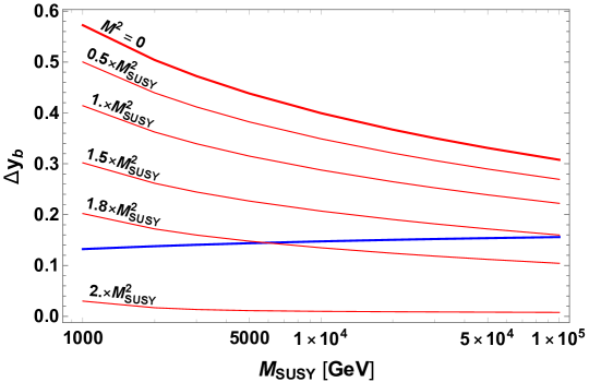
Figure 4: The $M_{\rm SUSY}$ dependence of the required and maximal SUSY threshold corrections. The blue line shows the required SUSY threshold correction for realizing the $SO(10)$ Yukawa unification. The red lines show the maximal SUSY threshold corrections with different values of $M^{2}$. The thick red line which is the case with $M^{2}=0$ corresponds to the maximal SUSY threshold correction in the range of $0\leq M^{2}<2M_{\rm SUSY}^{2}$.

The blue line shows the required SUSY threshold correction for realizing the $SO(10)$ Yukawa unification, while the red ones show the maximal SUSY threshold corrections with different values of $M^{2}$, calculated from the above discussion. The thick red line which is the case with $M^{2}=0$ corresponds to the maximal SUSY threshold correction in the range of $0\leq M^{2}<2M_{\rm SUSY}^{2}$. Here, we assume that $M_{3}=M_{\rm SUSY}$ as in our setup, $C_{0}(|M_{3}|^{2},m_{\tilde{b}_{L}}^{2},m_{\tilde{b}_{R}}^{2})=-\frac{1}{2M_{\rm SUSY}^{2}}$, and $\delta m^{2}_{bt}=0.08M_{\rm SUSY}^{2}$. The second assumption is valid when $m_{\tilde{b}_{L,R}}^{2}\simeq M_{\rm SUSY}^{2}$. Note that $\delta m^{2}_{bt}$ is not important to obtain the maximal value of $\Delta y_{b}$ unless this is enough large to compete the other contributions. We found that $\delta m^{2}_{bt}$ is less than $0.1M_{\rm SUSY}^{2}$ in our calculation since we use the universal sfermion mass as the input at the GUT scale.

We can find important results from Fig. 4. First, the maximal SUSY threshold correction is larger than the required one when $M_{\rm SUSY}\leq 100$ TeV, and then, we can find the parameter set which realizes the required SUSY threshold correction. Second, the maximal SUSY threshold correction decreases when $M^{2}$ becomes large. This means that $\Delta y_{b}$ is dominated by the contribution from $\mu$, as one can understand from the plot with $M^{2}=2M_{\rm SUSY}^{2}$ case, namely, $\mu_{\rm max}=0$ case. Therefore, we can obtain the required SUSY threshold correction from the appropriate values of $m_{h_{u}}^{2}$ and $m_{h_{d}}^{2}$. Third, as the SUSY scale increases, the required SUSY threshold correction increases, while the maximal SUSY threshold correction decreases. This is because the rough expression for the maximal value of $\Delta y_{b}$ is

$$\Delta y_{b}\sim-\frac{2}{3}\frac{\alpha_{s}}{\pi}M_{\rm SUSY}\bigl{(}\sqrt{2}M_{\rm SUSY}y_{b}\tan\beta\bigr{)}\left(-\frac{1}{2M_{\rm SUSY}^{2}}\right)\propto\alpha_{s}y_{b}\tan\beta,$$ (58)

and this combination becomes small when the SUSY scale become high. Therefore, we can expect that there is an intersection point between the required and maximal SUSY threshold corrections. This means that there is an upper bound on the SUSY scale when we consider the $SO(10)$ Yukawa unification, although its bound is expected to be far above $M_{\rm SUSY}=100$ TeV.

Finally, we comment on the situation in which we do not consider in the above discussion. If $m_{\tilde{\tau}_{L}}^{2}+m_{\tilde{\tau}_{R}}^{2}<2M_{\rm SUSY}^{2}-\frac{m_{Z}^{2}}{2}\left(\tan^{2}\beta-1\right)$ due to the small $m_{\tilde{\tau}_{R}}^{2}$ through the MSSM RGE, the maximal value of $|m_{h_{d}}^{2}|$ is $m_{\tilde{\tau}_{L}}^{2}+m_{\tilde{\tau}_{R}}^{2}$ from the CCB constraint of $(\hat{A}_{e})_{33}$ when $m_{h_{d}}^{2}<0$. In this case, the maximal value of $|m_{h_{u}}^{2}|$ is modified as

$$|m_{h_{u}}^{2}|=m_{\tilde{\tau}_{L}}^{2}+m_{\tilde{\tau}_{R}}^{2}+\frac{m_{Z}^{2}}{2}\left(\tan^{2}\beta-1\right)$$ (59)

in order to satisfy the EWSB constraints. This is smaller than $2M_{\rm SUSY}^{2}$, and therefore, the maximal value of $\mu$ is also smaller than the above case. Note that in this case, since $|a_{b}|_{\rm max}=\sqrt{y_{b}\,\delta m^{2}_{b\tau}}$ where $\delta m^{2}_{b\tau}\equiv m_{\tilde{b}_{L}}^{2}+m_{\tilde{b}_{R}}^{2}-\left(m_{\tilde{\tau}_{L}}^{2}+m_{\tilde{\tau}_{R}}^{2}\right)<2M_{\rm SUSY}^{2}$, we can safely ignore the contribution from $a_{b}$, according to the above results. Therefore, we can obtain the maximal $\Delta y_{b}$ from Fig. 4 straightforwardly. For example, when $|m_{h_{u}}^{2}|\simeq 1.5M_{\rm SUSY}^{2}$, predicted value of $\Delta y_{b}$ is around the red line with $M^{2}=0.5M_{\rm SUSY}^{2}$. However, $m_{\tilde{\tau}_{L}}^{2}+m_{\tilde{\tau}_{R}}^{2}$ is not far below $2M_{\rm SUSY}^{2}$ because of the input parameter at the GUT scale. Therefore, we can conclude that the maximal SUSY threshold correction is always larger than the required one when $M_{\rm SUSY}\leq 100$ TeV.

References

- [1] G. Aad et al. [ATLAS Collaboration], Phys. Lett. B 716, 1 (2012) [arXiv:1207.7214 [hep-ex]]; S. Chatrchyan et al. [CMS Collaboration], Phys. Lett. B 716, 30 (2012) [arXiv:1207.7235 [hep-ex]].
- [2] N. Cabibbo, Phys. Rev. Lett. 10, 531 (1963); M. Kobayashi and T. Maskawa, Prog. Theor. Phys. 49, 652 (1973).
- [3] L. J. Hall, V. A. Kostelecky and S. Raby, Nucl. Phys. B 267, 415 (1986).
- [4] H. Georgi and S. L. Glashow, Phys. Rev. Lett. 32, 438 (1974).
- [5] K. Abe et al. [Super-Kamiokande Collaboration], Phys. Rev. D 95, 012004 (2017) [arXiv:1610.03597 [hep-ex]]; K. Abe et al. [Super-Kamiokande Collaboration], Phys. Rev. D 96, 012003 (2017) [arXiv:1705.07221 [hep-ex]].
- [6] Y. Achiman and C. Merten, Nucl. Phys. B 584, 46 (2000) [hep-ph/0004023]; Y. Achiman and M. Richter, Phys. Lett. B 523, 304 (2001) [hep-ph/0107055]; J. R. Ellis, D. V. Nanopoulos and J. Walker, Phys. Lett. B 550, 99 (2002) [hep-ph/0205336]; N. Maekawa and Y. Muramatsu, Phys. Lett. B 767, 398 (2017) [arXiv:1601.04789 [hep-ph]].
- [7] H. Georgi, AIP Conf. Proc. 23, 575 (1975); H. Fritzsch and P. Minkowski, Annals Phys. 93, 193 (1975).
- [8] P. Minkowski, Phys. Lett. 67B, 421 (1977); M. Gell-Mann, P. Ramond and R. Slansky, Conf. Proc. C 790927, 315 (1979) [arXiv:1306.4669 [hep-th]]; T. Yanagida, Conf. Proc. C 7902131, 95 (1979); S. L. Glashow, NATO Sci. Ser. B 61, 687 (1980); R. N. Mohapatra and G. Senjanovic, Phys. Rev. Lett. 44, 912 (1980).
- [9] W. Konetschny and W. Kummer, Phys. Lett. 70B, 433 (1977); T. P. Cheng and L. F. Li, Phys. Rev. D 22, 2860 (1980); G. Lazarides, Q. Shafi and C. Wetterich, Nucl. Phys. B 181, 287 (1981); J. Schechter and J. W. F. Valle, Phys. Rev. D 22, 2227 (1980); R. N. Mohapatra and G. Senjanovic, Phys. Rev. D 23, 165 (1981).
- [10] A. L. Kagan and C. H. Albright, Phys. Rev. D 38, 917 (1988); T. Banks, Nucl. Phys. B 303, 172 (1988); E. Ma, Phys. Rev. D 39, 1922 (1989).
- [11] R. Hempfling, Phys. Rev. D 49, 6168 (1994); L. J. Hall, R. Rattazzi and U. Sarid, Phys. Rev. D 50, 7048 (1994) [hep-ph/9306309]; M. Carena, M. Olechowski, S. Pokorski and C. E. M. Wagner, Nucl. Phys. B 426, 269 (1994) [hep-ph/9402253]; H. Baer and J. Ferrandis, Phys. Rev. Lett. 87, 211803 (2001) [hep-ph/0106352]; T. Blazek, R. Dermisek and S. Raby, Phys. Rev. Lett. 88, 111804 (2002) [hep-ph/0107097]; K. Tobe and J. D. Wells, Nucl. Phys. B 663, 123 (2003) [hep-ph/0301015]; D. Auto, H. Baer, C. Balazs, A. Belyaev, J. Ferrandis and X. Tata, JHEP 0306, 023 (2003) [hep-ph/0302155]; M. Albrecht, W. Altmannshofer, A. J. Buras, D. Guadagnoli and D. M. Straub, JHEP 0710, 055 (2007) [arXiv:0707.3954 [hep-ph]]; S. Antusch and M. Spinrath, Phys. Rev. D 78, 075020 (2008) [arXiv:0804.0717 [hep-ph]]; S. Antusch and M. Spinrath, Phys. Rev. D 79, 095004 (2009) [arXiv:0902.4644 [hep-ph]]; A. Crivellin and C. Greub, Phys. Rev. D 87, 015013 (2013) [Erratum: Phys. Rev. D 87, 079901 (2013)] [arXiv:1210.7453 [hep-ph]]. A. Anandakrishnan, S. Raby and A. Wingerter, Phys. Rev. D 87, 055005 (2013) [arXiv:1212.0542 [hep-ph]].
- [12] T. Blazek, S. Raby and S. Pokorski, Phys. Rev. D 52, 4151 (1995) [hep-ph/9504364]; J. Ferrandis and N. Haba, Phys. Rev. D 70, 055003 (2004) [hep-ph/0404077]; A. Crivellin and U. Nierste, Phys. Rev. D 79, 035018 (2009) [arXiv:0810.1613 [hep-ph]]; A. Crivellin, L. Hofer, U. Nierste and D. Scherer, Phys. Rev. D 84, 035030 (2011) [arXiv:1105.2818 [hep-ph]].
- [13] A. Crivellin and U. Nierste, Phys. Rev. D 81, 095007 (2010) [arXiv:0908.4404 [hep-ph]].
- [14] A. Crivellin, L. Hofer and J. Rosiek, JHEP 1107, 017 (2011) [arXiv:1103.4272 [hep-ph]].
- [15] M. Drees, M. Gluck and K. Grassie, Phys. Lett. 157B, 164 (1985); J. F. Gunion, H. E. Haber and M. Sher, Nucl. Phys. B 306, 1 (1988); H. Komatsu, Phys. Lett. B 215, 323 (1988); P. Langacker and N. Polonsky, Phys. Rev. D 50, 2199 (1994) [hep-ph/9403306]; J. A. Casas, A. Lleyda and C. Munoz, Nucl. Phys. B 471, 3 (1996) [hep-ph/9507294]; J. A. Casas and S. Dimopoulos, Phys. Lett. B 387, 107 (1996) [hep-ph/9606237].
- [16] J. R. Ellis and M. K. Gaillard, Phys. Lett. 88B, 315 (1979).
- [17] M. Tanabashi et al. [Particle Data Group], Phys. Rev. D 98, 030001 (2018).
- [18] K. G. Chetyrkin, J. H. Kuhn and M. Steinhauser, Comput. Phys. Commun. 133, 43 (2000) [hep-ph/0004189].
- [19] H. Arason, D. J. Castano, B. Keszthelyi, S. Mikaelian, E. J. Piard, P. Ramond and B. D. Wright, Phys. Rev. D 46, 3945 (1992).
- [20] M. E. Machacek and M. T. Vaughn, Nucl. Phys. B 222, 83 (1983); M. E. Machacek and M. T. Vaughn, Nucl. Phys. B 236, 221 (1984); M. E. Machacek and M. T. Vaughn, Nucl. Phys. B 249, 70 (1985).
- [21] M. x. Luo and Y. Xiao, Phys. Rev. Lett. 90, 011601 (2003) [hep-ph/0207271].
- [22] A. V. Bednyakov, A. F. Pikelner and V. N. Velizhanin, Phys. Lett. B 722, 336 (2013) [arXiv:1212.6829 [hep-ph]].
- [23] K. G. Chetyrkin and M. F. Zoller, JHEP 1304, 091 (2013) [Erratum: JHEP 1309, 155 (2013)] [arXiv:1303.2890 [hep-ph]].
- [24] S. Antusch and V. Maurer, JHEP 1311, 115 (2013) [arXiv:1306.6879 [hep-ph]]; V. K. M. Maurer, doi:10.5451/unibas-006387307
- [25] S. P. Martin and M. T. Vaughn, Phys. Lett. B 318, 331 (1993) [hep-ph/9308222].
- [26] S. P. Martin and M. T. Vaughn, Phys. Rev. D 50, 2282 (1994) [Erratum: Phys. Rev. D 78, 039903 (2008)] [hep-ph/9311340].
- [27] G. F. Giudice and G. Ridolfi, Z. Phys. C 41, 447 (1988); M. Olechowski and S. Pokorski, Phys. Lett. B 214, 393 (1988); B. Ananthanarayan, G. Lazarides and Q. Shafi, Phys. Rev. D 44, 1613 (1991); H. Arason, D. Castano, B. Keszthelyi, S. Mikaelian, E. Piard, P. Ramond and B. Wright, Phys. Rev. Lett. 67, 2933 (1991); S. Kelley, J. L. Lopez and D. V. Nanopoulos, Phys. Lett. B 274, 387 (1992).
- [28] F. Gabbiani, E. Gabrielli, A. Masiero and L. Silvestrini, Nucl. Phys. B 477, 321 (1996) [hep-ph/9604387].
- [29] M. Bona et al. [UTfit Collaboration], Phys. Rev. Lett. 97, 151803 (2006) [hep-ph/0605213]; M. Bona et al. [UTfit Collaboration], JHEP 0803, 049 (2008) [arXiv:0707.0636 [hep-ph]];
- [30] P. Paradisi, JHEP 0510, 006 (2005) [hep-ph/0505046]; M. Arana-Catania, S. Heinemeyer and M. J. Herrero, Phys. Rev. D 88, 015026 (2013) [arXiv:1304.2783 [hep-ph]].
- [31] K. Inoue, A. Kakuto, H. Komatsu and S. Takeshita, Prog. Theor. Phys. 67, 1889 (1982).