Simple Pose: Rethinking and Improving a Bottom-up Approach
for Multi-Person Pose Estimation

Abstract

We rethink a well-known bottom-up approach for multi-person pose estimation and propose an improved one. The improved approach surpasses the baseline significantly thanks to (1) an intuitional yet more sensible representation, which we refer to as body parts to encode the connection information between keypoints, (2) an improved stacked hourglass network with attention mechanisms, (3) a novel focal L2 loss which is dedicated to “hard” keypoint and keypoint association (body part) mining, and (4) a robust greedy keypoint assignment algorithm for grouping the detected keypoints into individual poses. Our approach not only works straightforwardly but also outperforms the baseline by about 15$\%$ in average precision and is comparable to the state of the art on the MS-COCO test-dev dataset. The code and pre-trained models are publicly available online.

Introduction

The problem of multi-person pose estimation aims at recognizing and localizing the anatomical keypoints (or body joints) of all persons in a given image. Considerable progress has been made in this field, benefiting from the development of more powerful convolutional neural networks (CNNs), such as ResNet (?) and DenseNet (?), and more representative benchmarks, such as MS-COCO (?).

Existing approaches tackling this problem can be divided into two categories: top-down and bottom-up. The top-down approaches, e.g. (?; ?; ?), usually employ a state-of-the-art (SOTA) detector, such as SSD (?), to capture all the persons from the image first. Then, the cropped persons are resized and fed into the SOTA pose estimator designed for a single person, e.g. (?; ?; ?). In contrast, the bottom-up approaches, e.g. (?; ?), directly infer the keypoints and the connection information between keypoints of all persons in the image without a human detector. Afterwards, the keypoints are grouped to form multiple human poses based on the inferred connection information.

Top-down approaches, e.g. (?; ?; ?), usually have complicated structures and low performance-cost ratios. Compared with them, the bottom-up approaches, e.g. (?; ?), can be more efficient in inference and independent of human detectors. However, they have to group the keypoints correctly. And the keypoint grouping (paring or association in other words) can be a big challenge, resulting in another bottleneck for real-time usage (?; ?). CMU-Pose (?), PersonLab (?) and PifPaf (?) use the greedy parsing algorithm to group detected keypoints into individual poses and break through the bottleneck to some extent.

It is worth mentioning that the approach proposed by (?) (referred to as CMU-Pose here for convenience) is the first bottom-up approach to perform the task of multi-person pose estimation in the wild with high accuracy, and almost in real time. Our approach is mainly inspired by this work but is more intuitive yet more powerful. Hence, CMU-Pose is selected to be the baseline approach in this work.

The main contributions of this paper are summarized as follows: (1) we rethink the encoding of joint association, which is named as Part Affinity Fields (PAFs) (?), and propose a simplified yet more reasonable one, which we call body parts, (2) we present an improved stacked hourglass network with attention mechanisms to generate high-res and high-quality heatmaps, (3) we design a novel loss to help the network learn “hard” samples, and (4) we develop the greedy keypoint assignment algorithm.

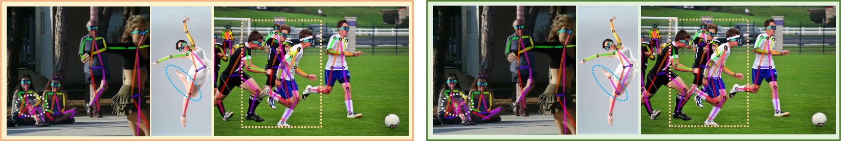
Figure 1: Qualitative comparison between our approach and CMU-Pose (?). Left: results produced by CMU-Pose. Right: our results. CMU-Pose works even when many people appear in the scene, but it suffers precision loss in keypoint localization and it can not detect or group the “hard” keypoints (such as the occluded keypoints) well. By comparison, our approach is more accurate in keypoint localization and more robust to complex poses and moderate overlaps.

Related Work and Rethinking

Single Person Pose Estimation

Classical approaches tackling the problem of person pose estimation are mainly based on the pictorial structures (?; ?) or the graphical models (?). They usually formulate this problem as a tree-structured or graphical model problem and detect the keypoints based on hand-crafted features (?). Recently, the SOTA approaches leverage advanced CNNs and more abundant datasets, making enormous progress in pose estimation. Here, we mainly discuss the CNN based approaches.

DeepPose (?) employs CNNs to solve this problem for the first time, by regressing the Cartesian coordinates of the joints (or keypoints) directly. By contrast, the work (?) presents CNNs to firstly predict the Gaussian response heatmaps of keypoints, and subsequently it obtains the keypoint positions via finding the local maximums in the heatmaps. Some up to date work, e.g. (?; ?), decomposes the problem of keypoint localization into two subproblems at each pixel location: (1) binary classification (0 or 1), and (2) regression of offset vector to the nearest keypoint.

Multi-Person Pose Estimation

Top-down approaches.

Most of the SOTA results have been achieved by the top-down approaches, such as CPN (?) and HRNet (?). Benefiting from the existing well-trained person detectors, the SOTA top-down approaches bypass the difficult subproblem of human body detection and turn the detection challenges into their advantages. However, they depend on the human detector heavily and they perform the task in two separate steps. The inference time will significantly increase if many people appear together.

Bottom-up approaches.

The bottom-up approaches, e.g. (?; ?; ?), are more efficient in keypoint inference and do not rely on the human detector. However, they tend to be less accurate. One main reason is that too large and too small persons in the image are difficult to detect at the same time (pose variation and feature map down-sampling make things even worse). Another main reason lies in the fact that the offset of only a few pixels away from the annotated keypoint location can lead to a big drop in the evaluation metrics (?) on the MS-COCO benchmark (?). On the contrary, the top-down approaches are immune to these challenges.

Some Rethinking

The topic of scale invariance in pose estimation is of great importance. Image pyramid (or multi-scale search in other words) technique is usually employed during testing to cover the human poses of different scales as much as possible (?; ?; ?), while the network is supervised at relatively a smaller scale range during training. Besides, some related work, e.g. (?; ?; ?), has designed special model structures to enhance the model invariance across scales.

High-res and high-quality feature maps (include the output heatmaps) are critical for accurate keypoint localization. Offset regression in PersonLab (?) and CornerNet (?), integral pose regression (?), and retaining (?) or even magnifying (?) the resolution of feature maps through the network are all good tries to relieve the precision loss (can not be avoided) caused by image or feature map resizing and small input or feature map size.

The encoding of connection (or association) information between keypoints is paid a lot of attention in some prior work, e.g. (?; ?; ?; ?). New representations bring about new ways of addressing problems. In this work, we only review the encoding of joint association named Part Affinity Fields (?) due to the limited space.

Another topic worthy of mention is the problem of imbalanced data: “positive” samples vs “negative” samples (between classes) and “easy” samples vs “hard” samples (within classes). A (Gaussian response) heatmap has most of its area equal to zero (background) and only a small portion of it corresponds to the Gaussian distribution (foreground). Thus, the spread of the Gaussian peaks should be controlled properly to balance the foreground and background. On the other hand, too many easy samples (such as Gaussian peaks of facial keypoints and easy background pixels) can prevent the network from learning the “hard” samples (such as Gaussian peaks corresponding to occluded keypoints or body parts) well. These two types of data imbalance problems are critical and should be addressed properly.

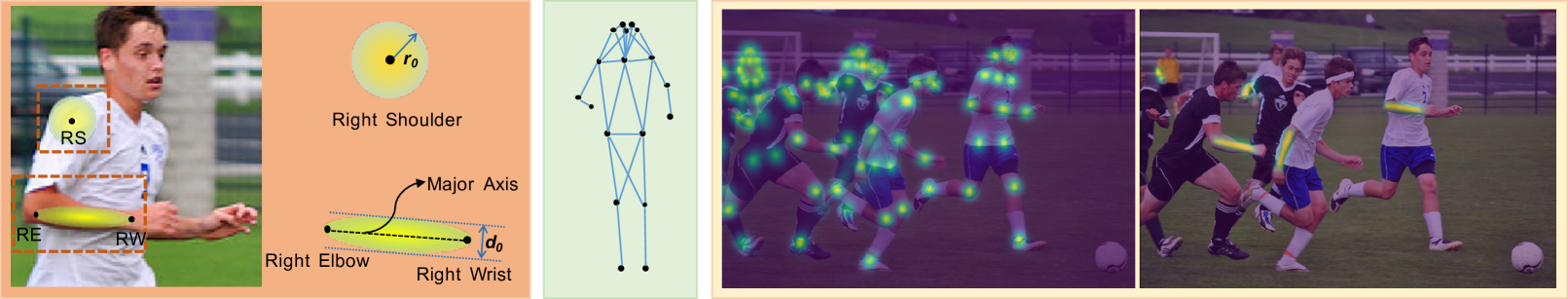
Figure 2: Definition of heatmaps. Left: examples of keypoint Gaussian peak and body part Gaussian peak. Middle: the human skeleton with redundant connections (which we refer to as redundant body parts). Right: examples of the inferred heatmaps by our network in practice.

Our Approach

We perform the task in three steps: (1) we predict the keypoint heatmaps and the body part heatmaps of all persons in a given image, (2) we get the candidate keypoints and body parts by performing Non-Maximum Suppression (NMS) on the inferred heatmaps, and (3) we perform the keypoint assignment algorithm and collect all individual poses.

Definition of Heatmaps

Considering the vague concept of keypoints and body parts, and human annotation variances (jitters), our network is supervised to regress the Gaussian responses (0$\sim$1 values) around the keypoint or body part area before obtaining the final localization, introducing the smooth mapping regularization and forcing the network to learn more features nearby.

The heatmaps here include keypoint heatmaps and body part heatmaps. Each pixel value in the keypoint heatmaps encodes the confidence that a nearest keypoint of a particular type occurs. We generate the ground truth keypoint heatmaps by putting unnormalized Gaussian distributions with a standard deviation ${{\sigma}_{k}}$ at all annotated keypoint positions. For example, the generated Gaussian peak of the right shoulder (RS) keypoint depicted in the Left of Figure 2.

The body part here refers to the body area which lies between the two adjacent keypoints (for instance, the forearm area in the Left of Figure 2). A set of body parts are used to encode the connection information between keypoints and extract the visual patterns of human skeleton (see the Middle of Figure 2). Since body part segmentations are not available and person masks only cover visible human body areas, we use an elliptical area to approximately represent the body part. We generate the ground truth body part heatmaps by putting unnormalized elliptical Gaussian distributions with a standard deviation ${{\sigma}_{p}}$ in all body part areas.

By the way, we map the pixel ${\bm{p}}$ at the location $(x,y)$ in the ${j}$-th ground truth heatmap to its original floating point location ${\bm{\tilde{p}}}(\tilde{x},\tilde{y})={\bm{\tilde{p}}}(x\cdot R+R/2-0.5,y\cdot R+R/2-0.5)$ in the input image, in which $R$ is the output stride, before generating the precise ground truth Gaussian peaks.

The PAFs proposed by (?) is a 2D vector field for each pixel in the limb area, which encodes the location and direction information of a limb. All the pixels within the approximate limb area (may include outliers of the limb) have the same ground truth value, which brings about vagueness or even conflicts to the information representation. The body part representation is more sensible and composite. Pixels near to the major axes of the body parts have higher confidence and vice versa. And we only need the half dimensions of PAFs to encode the keypoint connection information, reducing the demand for model capacity. During training, a single loss supervises the network to infer two kinds of Gaussian peaks, which have similar visual patterns and share the same formulation.

The standard deviations, ${{\sigma}_{k}}$ and ${{\sigma}_{p}}$, control the spread of the Gaussian peaks and they should be set properly to balance the foreground pixels and background pixels. The hyper-parameters ${{r}_{0}}$ and ${{d}_{0}}$ (see their meanings in Figure 2) determine the boundaries of the ground truth Gaussian peaks, truncating the unnormalized Gaussian distribution at a fixed value $thre$. It plays a role in our loss function.

Network Structure

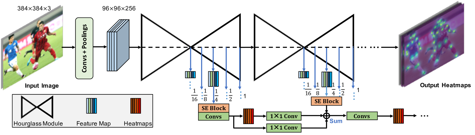
Figure 3: Identity Mapping Hourglass Network with spatial attention and channel attention mechanisms. The feature maps at 5 different scales (see Figure 4, the feature maps here refer to those surrounded by the blue dashed box in all down-sampling paths) are extracted from each (stage) hourglass module and they are used to produce heatmaps of different scales. Only the heatmap regression at the 1/4 scale is illustrated due to space limitation. The regressed feature maps and heatmaps from the previous stage are transformed and reused in the next stage by element-wise addition (i.e., identity mappings).

Large “receptive fields” in CNN are critical for learning long range spatial relationships and can bring about accuracy improvement (?). On the other hand, the detailed information (in smaller receptive fields) is needed for fine-grained localization. To consolidate the global and local features, hourglass networks (?; ?) have been designed to capture the different spatial extent information of each keypoint and association between keypoints by repeated bottom-up and top-down inference. In this work, we select the hourglass network, designed for multi-person pose estimation in Associative Embedding (AE) (?), as the base model and present an improved one. The improved variant, which we call Identity Mapping Hourglass Network (IMHN), significantly outperforms the hourglass network in AE (?).

The proposed IMHN, whose structure is depicted in Figure 3, is fully convolutional. It takes an image of any shape as the input and outputs multi-scale keypoint and body part heatmaps of all persons (if any) in the scene simultaneously. Before fed into the stacked hourglass modules, the original input is down-sampled twofold by some convolutional layers and max- pooling layers.

A first order hourglass module is designed as shown in Figure 4. The down-sampling path reduces the spatial extent of the input feature map by half once and increases the number of the feature map channels $C$ by $N$ ($C=256$ and $N=128$ in all experiments unless mentioned otherwise). After replacing the dashed box in Figure 4 with another first order module, we get a second order module. A fourth order module can be made by repeating this operation and it is the default hourglass module to build the IMHN. Therefore, the feature map in the deepest path of our IMHN has 768 channels. Please note that we just follow the related work (?; ?) to use the fourth order hourglass module and the same $C$ and $N$, ensuring we can make fair comparisons.

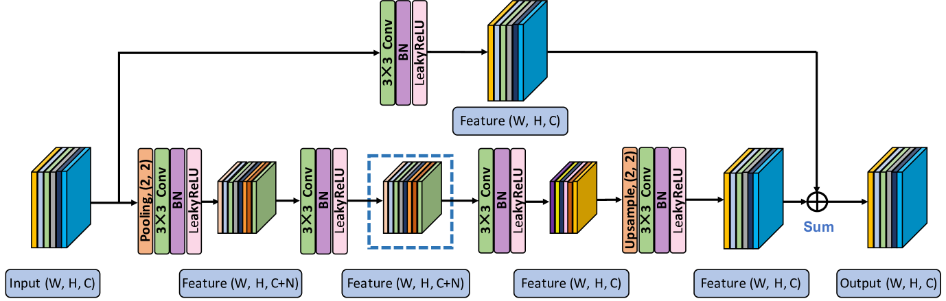
Figure 4: First order hourglass module. The two branches in this module extract different spatial features and merge them later by element-wise addition.

During training, multi-scale supervision (?) marked with blue arrows in Figure 3 is applied to supervise the fourth order stacked IMHN to infer heatmaps at 5 scales from coarse to fine, which explicitly introduces the “spatial attention” mechanism. Supervising the network at smaller scales can force the network to capture multi-scale structure information of each keypoint and body part. The low-res heatmaps can provide the guidance of location refinement in the subsequent high-res layers, contributing to the generation of high-quality and high-res heatmaps. Incidentally, the ground truth heatmaps at fractional scales are down-sampled from the full-size ones using adaptive average-pooling.

The feature map at a certain scale, which is used to regress the heatmaps at the same scale, is highly self-correlated, for it encodes pose structure information. An SE (squeeze and excitation) block (?) is inserted into each feature map at each scale to learn the channel relationships, which automatically introduces the “channel attention” mechanism. Here, we just employ existing techniques to quickly validate our thoughts.

Another important innovation in IMHN is that we add identity mappings between the same spatial extent feature maps and heatmaps across different stages (please refer to Figure 3). They can ease the network training experimentally: stabilizing different stages’ losses and helping the total loss converge faster.

Loss Functions

The L2 loss is frequently used to measure the distance between the predicted heatmaps and the target heatmaps, e.g. (?; ?; ?). To handle the “hard” keypoints, the work (?) proposes the L2 loss with online “hard” keypoint mining. Here, we present a novel loss, which we refer to as focal L2 loss, under the unified definition of keypoint and body part heatmaps, to deal with the two types of sample imbalance problems as introduced in Section Some Rethinking.

At each stage of the stacked IMHN, $K$ keypoint heatmaps and $P$ body part heatmaps are inferred at 5 different scales. A pixel value in the inferred heatmaps represents the confidence of being a certain category of keypoint or body part. Assuming the predicted score maps (or heatmaps) of size $w_{i}\times h_{i}$ at stage $t$ are ${{\bm{S}}^{t}}=\left(\bm{S}_{1}^{t},\bm{S}_{2}^{t},\cdots,\bm{S}_{K+P}^{t}\right)$, $t\in\left\{1,2,\cdots,T\right\}$, where $T$ is the total number of stacked hourglass modules. Supposing the ground truth heatmaps of the same size are ${{\bm{S}}^{*}}=\left(\bm{S}_{1}^{*},\bm{S}_{2}^{*},\cdots,\bm{S}_{K+P}^{*}\right)$ and the Gaussian peak generation function is ${G}$. Let $\bm{S}_{j}^{*}(\bm{p})$ denote the ground truth score at the pixel location $\bm{p}(x,y)\in{{\mathbb{R}}^{w_{i}\times h_{i}}}$ in the ${j}$-th heatmap, we compute $\bm{S}_{j}^{*}(p)$ as:

$$\bm{S}_{j}^{*}\left(\bm{p}\right)=\left\{\begin{array}[]{lr}G({x,y|R,\sigma}_{k},r_{0}),\quad 1\leq j\leq K\\ G({x,y|R,\sigma}_{p},d_{0}),\quad K<j\leq K+P.\end{array}\right.$$ (1)

We define $\bm{Sd}_{j}^{t}\left(p\right)$:

$$\bm{Sd}_{j}^{t}\left(p\right)=\left\{\begin{array}[]{lr}\bm{S}_{j}^{t}\left(\bm{p}\right)-\alpha,\>\>\bm{S}_{j}^{*}\left(\bm{p}\right)>thre\\ 1-\bm{S}_{j}^{t}\left(\bm{p}\right)-\beta,\>\>\>else,\end{array}\right.$$ (2)

where $thre$ (mentioned in Section Definition of Heatmaps) is the threshold to distinguish between the foreground heatmap pixels and the background heatmap pixels, and $\alpha$, $\beta$ are compensation factors to reduce the punishment of easy samples (both easy foreground pixels and easy background pixels) so that we can make full use of the training data.

The focal L2 loss (${\cal FL}$) between the predicted heatmaps and target heatmaps of size $w_{i}\times h_{i}$ at stage $t$ is computed as follow:

$$\begin{array}[]{lr}{\cal FL}_{i}^{t}=\sum\limits_{j=1}^{K+P}{\sum\limits_{\bm{p}\in{{\mathbb{R}}^{w_{i}\times h_{i}}}}\left[\eta\cdot{\mathbb{I}}\left(j\leq K\right)+1\right]\cdot{\bm{W}\left(\bm{p}\right)}}\\ \quad\quad\quad\quad\cdot\left\|\bm{S}_{j}^{t}\left(\bm{p}\right)-\bm{S}_{j}^{*}\left(\bm{p}\right)\right\|_{2}^{2}\cdot\left\|1-\bm{Sd}_{j}^{t}\left(\bm{p}\right)\right\|_{2}^{2},\\ \end{array}$$ (3)

here, $\bm{W}$ is a binary mask with $\bm{W}\left(\bm{p}\right)=0$ when the annotation is missing at the location $\bm{p}$, $\mathbb{I}$ is the indicator function, and $\eta$ is the hyper-parameter to balance the keypoint heatmap loss and body part heatmap loss. The presented scaling factor term $\left\|1-\bm{Sd}_{j}^{t}\left(\bm{p}\right)\right\|_{2}^{2}$ implies two prior information: the inferred responses (scores) of easy foregrounds tend to be high (close to 1, e.g.,0.9); the inferred responses of easy backgrounds tend to be low (usually less than 0.01 in practice). Thus, it can automatically down-weight the contribution of easy samples during training, which is inspired by Focal Loss (?).

In this work, we set ${{\sigma}_{k}}=9$, ${{\sigma}_{p}}=7$, $thre=0.01$ for the gradient balance between the foreground and background pixels, and we set $\eta=2$ accordingly. In addition, we set $\alpha=0.1$ and $\beta=0.02$ roughly ($\alpha$ and $\beta$ should be set close to $0$ and $\alpha>\beta>0$). For better understandings of the important hyper-parameters, we provide more descriptions.

As for the standard deviations of keypoint and body part Gaussian peaks, i.e., ${{\sigma}_{k}}$ and ${{\sigma}_{p}}$, if we set them too small, the accurate localization information is preserved but the inferred responses at these peaks tend to be low, resulting in more false negatives. On the other hand, if we set them too big, the Gaussian peaks spread so flat that the localization information tends to become vague at inference time, harming localization precision (using offset regression may relieve this problem). As to the hyper-parameter $thre$, it is set to 0.01 to significantly compress the loss of a mass of easy background pixels. After the network becomes able to distinguish the background well, then, the loss of the foreground starts to play a major role in the network learning.

The total loss of the stacked IMHN across 5 different scales can be written as:

$${\cal L}={\sum_{t=1}^{T}{\sum_{i=1}^{5}{{{\lambda}_{i}^{t}\cdot}{\cal FL}_{i}^{t}}}}/{\sum_{i=1}^{5}{{\lambda}_{i}^{t}}},$$ (4)

in which $\lambda_{1}^{t}=1$, ${{\lambda}_{2}^{t}}=2$, ${{\lambda}_{3}^{t}}=4$, ${{\lambda}_{4}^{t}}=16$ and ${{\lambda}_{5}^{t}}=64$ are presented for the balance between losses at different scales. Now, “hard” keypoints and “hard” keypoint association (as the form of body parts ) can be learned better with the help of the proposed loss under our heatmap definition.

Keypoint Assignment Algorithm

The candidate keypoints are assigned provided that the candidate body parts are assembled into corresponding human skeletons. We perform NMS (3 $\times$ 3 window) on the predicted heatmaps to find the candidate keypoints. Then, we obtain the candidate body parts that lie between the candidate adjacent keypoints, and calculate their scores that represent the confidence of being body parts, by sampling a set of Gaussian responses within the body part areas. After that, the candidate body parts of the same type are sorted in descending order according to the weighted scores of body parts and connected keypoints. Consequently, $K$ sets of keypoints $J=\left\{J{{s}_{1}},J{{s}_{2}},\cdots,J{{s}_{K}}\right\}$ and $P$ sets of body parts $L=\left\{L{{s}_{1}},L{{s}_{2}},\cdots,L{{s}_{P}}\right\}$ are obtained.

Each element ${{l}_{i,j}}\in L{{s}_{i}}$ is a body part instance with type ID ${i}$, connected keypoints and weighted score ${S}_{l_{i,j}}$. Here, one candidate keypoint can not be shared by two or more body parts of the same type, i.e., $\forall$ $j$, $k$ and $m$, $\left\{l_{i,j},l_{i,k}\right\}\subseteq Ls_{i}$ and $j\neq k$, we ensure that ${{l}_{i,j}}\cap{{l}_{i,k}}\cap Js_{m}=\phi$, where $Js_{m}\in J$. This rule works in analogy to the NMS for candidate bounding boxes in object detection task.

Supposing the set of assembled human poses is $H=\left\{{{h}_{1}},{{h}_{2}},{{h}_{3}},\cdots\right\}$, in which ${{h}_{n}}\in H$ represents a single person pose. Then, ${{h}_{n}}$ has $1\sim P$ assigned body parts, corresponding type IDs and total score ${S}_{{h}_{n}}$. Our goal is to select the proper candidate body parts and find the best grouping strategy between the body parts in $L{{s}_{1}},L{{s}_{2}},\cdots,L{{s}_{P}}$, such that $\sum_{{h}_{n}\epsilon H}{{S}_{{h}_{n}}}$ reaches to its global maximum. Instead of solving the problem of global graph matching globally, CMU-Pose (?) proposes a greedy algorithm upon a minimum spanning tree (MST) of human skeleton to match the adjacent tree nodes independently at only a fraction of the original computational cost.

We follow the greedy strategy in CMU-Pose and assemble the human skeletons (see the Middle of Figure 2) by matching adjacent body parts independently. Our keypoint assignment algorithm is based on several simple connection rules. As redundant body parts are introduced in our human skeleton, the assembled body parts having lower scores are removed by the body parts having higher scores, which share the same connected keypoint(s).

Table 1: Results on the MS-COCO 2017 validation set.

ID	Method	Input	Stride	${\cal FL}$	AP	ID	Method	Input	Stride	${\cal FL}$	AP
1	CMU-Pose (6-stage CMU-Net)	368	8	N	56.0	12	3-stage IMHN, w/ MST	384	4	Y	65.1
2	AE (4-stage Hourglass, + val data)	512	4	N	59.7	13	4-stage IMHN	384	4	N	64.5
3	Top-down∗ (8-stage Hourglass)	256	4	N	66.9	14	4-stage IMHN	384	4	Y	67.3
4	Ours (3-stage CMU-Net)	368	8	N	56.5	15	4-stage IMHN, + val data	384	4	Y	72.3
5	Ours (3-stage CMU-Net)	368	8	Y	60.7	16	4-stage IMHN plus	512	4	Y	69.1
6	Ours (4-stage Hourglass)	512	4	N	60.0	17	4-stage IMHN plus, + val data	512	4	Y	74.1
7	3-stage IMHN	384	4	N	61.5	18	4-stage IMHN, one scale	768	4	Y	63.4
8	3-stage IMHN	384	4	Y	65.8	19	4-stage IMHN plus, one scale	768	4	Y	65.9
9	3-stage IMHN, w/o spatial attention	384	4	Y	64.6	20	PifPaf (ResNet-101), one scale	801	8	–	65.7
10	3-stage IMHN, w/o channel attention	384	4	Y	65.4	21	PersonLab∗, one scale	801	8	–	61.2
11	3-stage IMHN, ${\cal FL}$ only for keypoint	384	4	Y	64.2	22	PersonLab∗, one scale	1401	8	–	66.5

Table 2: Results on the MS-COCO 2017 test-dev set.

Method	Backbone	Pretrain	Train Input	Test Input	Refine	AP	APM	APL	AR	AR50
Bottom-up: multi-person keypoint detection and grouping
CMU-Pose (baseline) (?)	6-stage CMU-Net	N	368$\times$368	$\sim$ 3682	N	52.9	50.9	57.2	57.0	79.2
CMU-Pose∗ (?)	6-stage CMU-Net	N	368$\times$368	$\sim$ 3682	Y	61.8	57.1	68.2	66.5	87.2
AE∗ (?)	4-stage Hourglass	N	512$\times$512	$\sim$ 5122	Y	65.5	60.6	72.6	70.2	89.5
PersonLab∗ (?)	ResNet-101	Y	801$\times$801	$\sim$ 14012	N	67.8	63.0	74.8	74.5	92.2
PifPaf (?)	ResNet-101	Y	401$\times$401	$\sim$ 6412	N	64.9	60.6	71.2	70.3	90.2
PifPaf∗ (?)	ResNet-152	Y	401$\times$401	$\sim$ 6412	N	66.7	62.4	72.9	72.2	90.9
Ours-1, w/ ${\cal FL}$	3-stage CMU-Net	N	368$\times$368	$\sim$ 3682	N	59.3	56.2	63.8	63.5	84.6
Ours-2, w/ ${\cal FL}$	3-stage IMHN	N	384$\times$384	$\sim$ 3842	N	65.2	63.7	68.5	69.8	87.7
Ours-3, w/ ${\cal FL}$	4-stage IMHN	N	384$\times$384	$\sim$ 3842	N	66.2	66.4	66.6	71.2	88.6
Ours-4 (final), w/ ${\cal FL}$	4-stage IMHN plus	N	512$\times$512	$\sim$ 5122	N	68.1	66.8	70.5	72.1	88.2
Ours-5, w/ ${\cal FL}$	4-stage IMHN plus	N	512$\times$512	$\sim$ 3842	N	67.6	64.5	72.6	71.3	87.6
Top-down: human detection and single-person keypoint detection
G-RMI∗ (?)	RseNet-101	Y	353$\times$257	353$\times$257	–	64.9	62.3	70.0	69.7	88.7
CPN∗ (?)	ResNet-Inception	Y	384$\times$288	384$\times$288	–	72.1	68.7	77.2	78.5	95.1
HRNet-W48∗ (?)	HRNet-W48	Y	384$\times$288	384$\times$288	–	75.5	71.9	81.5	80.5	95.7

Experiments

Implementation Details

Dataset and evaluation metrics.

Our models are trained and evaluated on the MS-COCO dataset (?), which consists of the training set (includes around 60K images), the test-dev set (includes around 20K images) and the validation set (includes 5K images). The MS-COCO evaluation metrics, OKS-based average precision (AP) and average recall (AR), are used to evaluate the results.

Training details.

The training images with random transformations are cropped and resized to the fixed spatial extent of 384 $\times$ 384. And the generated ground truth heatmaps have the size of 96 $\times$ 96. We implement both the 3-stage IMHN and 4-stage IMHN using Pytorch. To train the networks, we use the SGD optimizer with the learning rate of 1e-4 (multiplied by 0.2 for every 15 epochs), the momentum of 0.9, the batch size of 32 and the weight decay of 5e-4. We train the IMHNs with L2 loss first and then continue to train them with the focal L2 loss (${\cal FL}$) until the performance refuses to improve. The last but not least, our networks are in mixed precision to reduce the memory consumption and speed up the experiments. The implemented 4-stage IMHN (see Ours-3 in Table 2) can be trained at the speed of 33 FPS with 4 RTX 2080TI GPUs, and we train it for about 3 days.

Testing details.

We first resize and pad the input image so that it fits the network. Then, the input image is inferred at multiple scales (for example, $\times$0.5, $\times$1, $\times$1.5, $\times$2) with flip augmentation. Next, the inferred heatmaps are averaged across scales (i.e., multi-scale search). After collecting the poses from the heatmaps via the keypoint assignment algorithm, we sort them in descending order according to their scores in heatmaps. To compare equally, we have run the released models of CMU-Pose (?), AE (?) and PifPaf (?), obtaining their results without the refinement for detected person poses.

Results and Analyses

Results on the MS-COCO dataset.

We have trained all our networks from scratch only with the MS-COCO data. The hyper-parameters of our approach are tuned according to the performance on the validation set. We compare our approach with the state of the art in Tables 1 and 2. The backbone of 4-stage IMHN has nearly the same number of convolutional layers as ResNet-101 (?). Thus, we specially compare our networks with those based on ResNet-101 backbone in PersonLab (?) and PifPaf (?) impartially. The entries marked with “*” in Tables 1 and 2 are results reported in their original papers.

The notations in our tables are explained as follows: “Input” denotes the long edge of the test image, “Stride” is the ratio of the input image size to the output feature map size, “MST” is short for minimum spanning tree of human skeleton without redundant body parts, “CMU-Net” represents the cascaded CNN used in CMU-Pose (?), “Hourglass” denotes the hourglass network, “Refine” indicates whether or not the result is additionally refined by a single person pose estimator. The entry named “Top-down” in Table 1 is a top-down approach cited from CPN (?). It employs a SOTA human detector and an 8-stage hourglass network for single person pose estimation.

Inference speed.

The speed of our system is tested on the MS-COCO test-dev set (?) .

• Inference speed of our 4-stage IMHN with 512 $\times$ 512 input on one 2080TI GPU: 38.5 FPS (100$\%$ GPU-Util).

• Processing speed of the keypoint assignment algorithm that is implemented in pure Python and a single process on CPU: 5.2 FPS (has not been well accelerated).

Ablation studies.

Some examples of the qualitative comparison between our approach and CMU-Pose is illustrated in Figure 1. The detailed ablation experiments of our approach, numbered for clarity, are shown in Table 1. Experiments 1 and 4 use different encodings of keypoint association (PAFs and body parts respectively). They reveal that the encoding of body parts is better. According to experiments 2 and 6, our approach equipped with the same network and L2 loss is comparable to AE which utilizes validation data. The focal L2 loss can bring about a 3$\sim$4% AP improvement over the L2 loss (see experiment 5 vs 4, experiment 8 vs 7 and experiment 14 vs 13) under the same definition of heatmaps. Experiments 8 and 11 demonstrate doing “hard” keypoint and body part (keypoint association) mining meanwhile is better. The 3-stage IMHN can lead to around a 5% AP improvement compared with the 3-stage CMU-Net (see experiment 7 vs 4 and experiment 8 vs 5), and the 4-stage IMHN outperforms the 4-stage hourglass network (see experiment 13 vs 6) by a big margin, indicating IMNHs’ advantages.

The introduced “spatial attention” and “channel attention” mechanisms contribute 1.2$\%$ and 0.4$\%$ AP increase respectively to the 3-stage IMHN (see experiments 8, 9 and 10). The redundant connections in human skeleton bring about a 0.7$\%$ AP improvement according to the comparative experiments of 8 and 12. Bigger input size or feature map size and more stacks can improve the accuracy consistently according to the results in Table 1. Thus, we continue to train the model in experiment 14 with 512 $\times$ 512 input and more data augmentation, and obtain the model named “4-stage IMHN plus” in experiment 16. Further, the 4-stage IMHN is able to fit the MS-COCO train-val data at 74.1$\%$ AP (see experiment 17), indicating the big promotion space of our system.

Comparisons with the state of the art.

All the models compared in the tables are evaluated without model ensemble. Some SOTA top-down approaches may outperform all the SOTA bottom-up approaches including ours, but they all depend on advanced human detectors and use very powerful networks for single person pose estimation. According to the results, it is safe to conclude that our approach outperforms the baseline by a big margin (experiment 5 vs 1 in Table 1 and Ours-1 vs the baseline in Table 2) and even surpasses the TOP-DOWN approaches with equal level backbones (please refer to “Top-down” in Table 1 and “G-RMI” in Table 2).

Our approach has achieved comparable or even better results on both single scales (see the experiments with IDs 18$\sim$ 22 in Table 1) and multiple scales (see the results in Table 2), compared with the latest SOTA bottom-up approaches, PifPaf and PersonLab, under fair conditions. However, PersonLab benefits greatly from the big input size (see experiment 22 vs 21 in Table 1). It can be seen that PifPaf and Personlab are superior to our approach in keypoint average recall (AR). But our approach is superior to them when it comes to the robustness to person scales. Both PersonLab and PifPaf drop over 10$\%$ from AP^L metric to AP^M metric (see the entries in Table 2), while our approach (Ours-4) performs well regardless of the person scales, be they middle scales (M) and large scales (L). What is more, most of other work benefits greatly from the networks pre-trained for the ImageNet classification task (?), while we train networks from scratch (see experiment 17).

Referring to the results on the MS-COCO test-dev set in Table 2, the proposed techniques except for the designed IMHN bring about a 6.4% AP improvement (Ours-1 vs baseline). The 3-stage IMHN can lead to a 5.9$\%$ AP increase compared with the 3-stage CMU-Net (Ours-2 vs Ours-1). The 4-stage IMHN can further contribute a 1$\%$ AP improvement over the 3-stage IMHN. And our final model, “4-stage IMHN plus” with bigger input (means bigger output feature maps), brings about a 15.1% AP improvement in total over the baseline. Incidentally, our approach significantly outperforms CMU-Pose and AE, though they have additionally refined the results using a single person pose estimator.

Conclusions

In this paper, we rethink and develop a bottom-up approach for multi-person pose estimation. We provide some insights into valuable design choices: (1) doing hard sample mining of keypoint and keypoint association meanwhile, (2) using a powerful network to generate high-res and high-quality heatmaps, and (3) introducing the scale invariance across person scales, which are more critical to improve the performance. The experimental results have demonstrated the significant improvement achieved by our approach over the baseline (+15.1$\%$ AP on the MS-COCO test-dev dataset). To the best of our knowledge, our approach, which is straightforward and easy to follow, is the first bottom-up approach to provide both the source code and pre-trained models with over 67$\%$ AP on the MS-COCO test-dev dataset.

References

- [Andriluka, Roth, and Schiele 2009] Andriluka, M.; Roth, S.; and Schiele, B. 2009. Pictorial structures revisited: People detection and articulated pose estimation. In 2009 IEEE Conference on Computer Vision and Pattern Recognition (CVPR), 1014–1021. IEEE.
- [Cao et al. 2017] Cao, Z.; Simon, T.; Wei, S. E.; and Sheikh, Y. 2017. Realtime multi-person 2d pose estimation using part affinity fields. In IEEE Conference on Computer Vision and Pattern Recognition (CVPR), 1302–1310.
- [Chen and Yuille 2014] Chen, X., and Yuille, A. L. 2014. Articulated pose estimation by a graphical model with image dependent pairwise relations. In Advances in Neural Information Processing Systems (NIPS), 1736–1744.
- [Chen et al. 2018] Chen, Y.; Wang, Z.; Peng, Y.; Zhang, Z.; Yu, G.; and Sun, J. 2018. Cascaded pyramid network for multi-person pose estimation. In IEEE Conference on Computer Vision and Pattern Recognition (CVPR), 7103–7112.
- [Chu et al. 2017] Chu, X.; Yang, W.; Ouyang, W.; Ma, C.; Yuille, A. L.; and Wang, X. 2017. Multi-context attention for human pose estimation. In Proceedings of the IEEE Conference on Computer Vision and Pattern Recognition (CVPR), 1831–1840.
- [Fischler and Elschlager 1973] Fischler, M. A., and Elschlager, R. A. 1973. The representation and matching of pictorial structures. In IEEE Transactions on Computers, volume 100, 67–92. IEEE.
- [He et al. 2016] He, K.; Zhang, X.; Ren, S.; and Sun, J. 2016. Deep residual learning for image recognition. In Proceedings of the IEEE Conference on Computer Vision and Pattern Recognition (CVPR), 770–778.
- [Hu, Shen, and Sun 2018] Hu, J.; Shen, L.; and Sun, G. 2018. Squeeze-and-excitation networks. In Proceedings of the IEEE Conference on Computer Vision and Pattern Recognition (CVPR), 7132–7141.
- [Huang et al. 2017] Huang, G.; Liu, Z.; van der Maaten, L.; and Weinberger, K. Q. 2017. Densely connected convolutional networks. In 2017 IEEE Conference on Computer Vision and Pattern Recognition (CVPR), 2261–2269. IEEE.
- [Iqbal and Gall 2016] Iqbal, U., and Gall, J. 2016. Multi-person pose estimation with local joint-to-person associations. In European Conference on Computer Vision (ECCV), 627–642. Springer.
- [Ke et al. 2018] Ke, L.; Chang, M.-C.; Qi, H.; and Lyu, S. 2018. Multi-scale structure-aware network for human pose estimation. In Proceedings of the European Conference on Computer Vision (ECCV), 713–728.
- [Kreiss, Bertoni, and Alahi 2019] Kreiss, S.; Bertoni, L.; and Alahi, A. 2019. Pifpaf: Composite fields for human pose estimation. In Proceedings of the IEEE Conference on Computer Vision and Pattern Recognition (CVPR), 11977–11986.
- [Law and Deng 2018] Law, H., and Deng, J. 2018. Cornernet: Detecting objects as paired keypoints. In Proceedings of the European Conference on Computer Vision (ECCV), 734–750.
- [Li et al. 2019] Li, W.; Wang, Z.; Yin, B.; Peng, Q.; Du, Y.; Xiao, T.; Yu, G.; Lu, H.; Wei, Y.; and Sun, J. 2019. Rethinking on multi-stage networks for human pose estimation. arXiv preprint arXiv:1901.00148.
- [Lin et al. 2014] Lin, T.-Y.; Maire, M.; Belongie, S.; Hays, J.; Perona, P.; Ramanan, D.; Dollár, P.; and Zitnick, C. L. 2014. Microsoft coco: Common objects in context. In European Conference on Computer Vision (ECCV), 740–755. Springer.
- [Lin et al. 2017] Lin, T.-Y.; Goyal, P.; Girshick, R.; He, K.; and Dollar, P. 2017. Focal loss for dense object detection. In 2017 IEEE International Conference on Computer Vision (ICCV), 2999–3007. IEEE.
- [Liu et al. 2016] Liu, W.; Anguelov, D.; Erhan, D.; Szegedy, C.; Reed, S.; Fu, C.-Y.; and Berg, A. C. 2016. Ssd: Single shot multibox detector. In European Conference on Computer Vision (ECCV), 21–37. Springer.
- [Newell, Huang, and Deng 2017] Newell, A.; Huang, Z.; and Deng, J. 2017. Associative embedding: End-to-end learning for joint detection and grouping. In Advances in Neural Information Processing Systems (NIPS), 2277–2287.
- [Newell, Yang, and Deng 2016] Newell, A.; Yang, K.; and Deng, J. 2016. Stacked hourglass networks for human pose estimation. In European Conference on Computer Vision (ECCV), 483–499. Springer.
- [Papandreou et al. 2017] Papandreou, G.; Zhu, T.; Kanazawa, N.; Toshev, A.; Tompson, J.; Bregler, C.; and Murphy, K. 2017. Towards accurate multi-person pose estimation in the wild. In 2017 IEEE Conference on Computer Vision and Pattern Recognition (CVPR), 3711–3719. IEEE.
- [Papandreou et al. 2018] Papandreou, G.; Zhu, T.; Chen, L.-C.; Gidaris, S.; Tompson, J.; and Murphy, K. 2018. Personlab: Person pose estimation and instance segmentation with a bottom-up, part-based, geometric embedding model. In The European Conference on Computer Vision (ECCV).
- [Pishchulin et al. 2016] Pishchulin, L.; Insafutdinov, E.; Tang, S.; Andres, B.; Andriluka, M.; Gehler, P. V.; and Schiele, B. 2016. Deepcut: Joint subset partition and labeling for multi person pose estimation. In Proceedings of the IEEE Conference on Computer Vision and Pattern Recognition (CVPR), 4929–4937.
- [Russakovsky et al. 2015] Russakovsky, O.; Deng, J.; Su, H.; Krause, J.; Satheesh, S.; Ma, S.; Huang, Z.; Karpathy, A.; Khosla, A.; Bernstein, M.; et al. 2015. Imagenet large scale visual recognition challenge. International Journal of Computer Vision 115(3):211–252.
- [Sun et al. 2018] Sun, X.; Xiao, B.; Wei, F.; Liang, S.; and Wei, Y. 2018. Integral human pose regression. In Proceedings of the European Conference on Computer Vision (ECCV), 529–545.
- [Sun et al. 2019] Sun, K.; Xiao, B.; Liu, D.; and Wang, J. 2019. Deep high-resolution representation learning for human pose estimation. In Proceedings of the IEEE Conference on Computer Vision and Pattern Recognition (CVPR), 5693–5703.
- [Tompson et al. 2014] Tompson, J.; Jain, A.; LeCun, Y.; and Bregler, C. 2014. Joint training of a convolutional network and a graphical model for human pose estimation. In Proceedings of the 27th International Conference on Neural Information Processing Systems-Volume 1 (NIPS), 1799–1807. MIT Press.
- [Toshev and Szegedy 2014] Toshev, A., and Szegedy, C. 2014. Deeppose: Human pose estimation via deep neural networks. In Proceedings of the IEEE Conference on Computer Vision and Pattern Recognition (CVPR), 1653–1660.
- [Wang et al. 2018] Wang, H.; An, W.; Wang, X.; Fang, L.; and Yuan, J. 2018. Magnify-net for multi-person 2d pose estimation. In IEEE International Conference on Multimedia and Expo (ICME), 1–6. IEEE.
- [Wei et al. 2016] Wei, S.-E.; Ramakrishna, V.; Kanade, T.; and Sheikh, Y. 2016. Convolutional pose machines. In Proceedings of the IEEE Conference on Computer Vision and Pattern Recognition (CVPR), 4724–4732.