dpVAEs: Fixing Sample Generation for Regularized VAEs

Abstract

Unsupervised representation learning via generative modeling is a staple to many computer vision applications in the absence of labeled data. Variational Autoencoders (VAEs) are powerful generative models that learn representations useful for data generation. However, due to inherent challenges in the training objective, VAEs fail to learn useful representations amenable for downstream tasks. Regularization-based methods that attempt to improve the representation learning aspect of VAEs come at a price: poor sample generation. In this paper, we explore this representation-generation trade-off for regularized VAEs and introduce a new family of priors, namely decoupled priors, or dpVAEs, that decouple the representation space from the generation space. This decoupling enables the use of VAE regularizers on the representation space without impacting the distribution used for sample generation, and thereby reaping the representation learning benefits of the regularizations without sacrificing the sample generation. dpVAE  leverages invertible networks to learn a bijective mapping from an arbitrarily complex representation distribution to a simple, tractable, generative distribution. Decoupled priors can be adapted to the state-of-the-art VAE regularizers without additional hyperparameter tuning. We showcase the use of dpVAEs  with different regularizers. Experiments on MNIST, SVHN, and CelebA demonstrate, quantitatively and qualitatively, that dpVAE  fixes sample generation for regularized VAEs.

1 Introduction

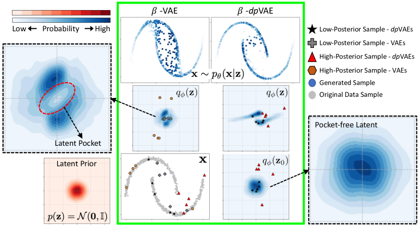
Figure 1: dpVAE  fixes sample generation for a regularized VAE. The green box shows $\beta$-VAE [20] (left column) and $\beta$-VAE with the proposed decoupled prior (right column), each trained on the two moons dataset. $\beta$-VAE: Top to bottom shows the generated samples (colors reflect probability of generation), the aggregate posterior $q_{\phi}(\mathbf{z})$ and the training samples. The low-posterior samples lie in the latent pockets of $q_{\phi}(\mathbf{z})$ (shown in enlarged section on the left) and correspond to off-manifold samples in the data space, and high-posterior samples correspond to latent leaks. The $\beta$-dpVAE  decouples the representation $\mathbf{z}$ and generation $\mathbf{z}_{0}$ spaces. The generation space is pocket-free and very close to standard normal, resulting in generating samples on the data manifold. Furthermore, the representation learning is well established in the representation space (see section 4.1 for more discussion).

Is it possible to learn a powerful generative model that matches the true data distribution with useful data representations amenable to downstream tasks in an unsupervised way? —This question is the driving force behind most unsupervised representation learning via state-of-the-art generative modeling methods (e.g. [58, 20, 23, 9]), with applications in artificial creativity [41, 37], reinforcement learning [21], few-shot learning [44], and semi-supervised learning [26]. A common theme behind such works is learning the data generation process using latent variable models [5, 1] that seek to learn representations useful for data generation; an approach known as analysis-by-synthesis [57, 39].

The Variational Autoencoder (VAE) [24, 46] marries latent variable models and deep learning by having independent, network-parameterized generative and inference models that are trained jointly to maximize the marginal log-likelihood of the training data. VAE introduces a variational posterior distribution that approximates the true posterior to derive a tractable lower bound on the marginal log-likelihood, a.k.a. the evidence lower bound (ELBO). The ELBO is then maximized using stochastic gradient descent by virtue of the reparameterization trick [24, 46]. Among the many successes of VAEs in representation learning tasks, VAE-based methods have demonstrated state-of-the-art performance for semi-supervised image and text classification tasks [33, 26, 49, 44, 43, 56].

Representation learning via VAEs is ill-posed due to the disconnect between the ELBO and the downstream task [54]. Specifically, optimizing the marginal log-likelihood is not always sufficient for good representation learning due to the inherent challenges rooted in the ELBO that result in the tendency to ignore latent variables and not encode information about the data in the latent space [54, 1, 58, 10, 22]. To improve the representations learned by VAEs, a slew of regularizations have been proposed. Many of these regularizers act on the VAE latent space to promote specific characteristics in the learned representations, such as disentanglement [58, 20, 23, 37, 8, 28] and informative latent codes [35, 2]. However, better representation learning usually sacrifices sample generation, which is manifested by a distribution mismatch between the marginal (a.k.a. aggregate) latent posterior and the latent prior. This mismatch results in latent pockets and leaks; a submanifold structure in the latent space (a phenomena demonstrated in Figure 1 and explored in more detail in section 4.1). Latent pockets contain samples that are highly supported under the prior but not covered by the aggregate posterior (i.e. low-posterior samples [47]), while latent leaks contain samples supported under the aggregate posterior but less likely to be generated under the prior (i.e. high-posterior samples). This behavior has been reported for VAE [47] but it is substantiated by augmenting the ELBO with regularizers (see Figure 1).

To address this representation-generation trade-off for regularized VAEs, we introduce the idea of decoupling the latent space for representation (representation space) from the space that drives sample generation (generation space); presenting a general framework for VAE regularization. To this end, we propose a new family of latent priors for VAEs — decoupled priors or dpVAEs  — that leverages the merits of invertible deep networks. In particular, dpVAE  transforms a tractable, simple base prior distribution in the generation space to a more expressive prior in the representation space that reflects the submanifold structure dictated by the regularizer. This is done using an invertible mapping that is jointly trained with the VAE’s inference and generative models. State-of-the-art VAE regularizers can thus be directly plugged in to promote specific characteristics in the representation space without impacting the distribution used for sample generation. We showcase, quantitatively and qualitatively, that dpVAE  with different state-of-the-art regularizers improve sample generation, without sacrificing their representation learning benefits.

It is worth emphasizing that, being likelihood-based models, VAEs are trained to put probability mass on all training samples, forcing the model to over-generalize [48], and generating blurry samples (i.e. off data manifold). This is in contrast to generative adversarial networks (GANs) [16] that generate outstanding image quality but lack the full data support [3]. dpVAE  is not expected to resolve the over-generalization problem in VAEs, but to mitigate poor sample quality resulting from regularization.

The contribution of this paper is fourfold:

• Analyze the latent submanifold structure induced by VAE regularizers.

• Introduce a decoupled prior family for VAEs as a general regularization framework that improves sample generation without sacrificing representation learning.

• Derive the dpVAE  ELBO of state-of-the-art regularized VAEs; $\beta$-dpVAE, $\beta$-TC-dpVAE, Factor-dpVAE, and Info-dpVAE.

• Demonstrate empirically on three benchmark datasets the improved generation performance and the preservation of representation characteristics promoted via regularizers without additional hyperparameter tuning.

2 Related Work

To improve sample quality, a family of approaches exist that combine the inference capability of VAEs and the outstanding sample quality of GANs [16]. Leveraging the density ratio trick [16, 51] that only requires samples, VAE-GAN hybrids in the latent (e.g. [38, 36]), data (e.g. [47, 48]), and joint (both latent and data e.g. [50]) spaces avoid restrictions to explicit posterior and/or likelihood distribution families, paving the way for marginals matching [47]. However, such hybrids scale poorly with latent dimensions, lack accurate likelihood bound estimates, and do not provide better quality samples than GAN variants [47]. Expressive posterior distributions can lead to better sample quality [38, 27] and are essential to prevent latent variables from being ignored in case of powerful generative models [10]. But results in [47] suggest that the posterior distribution is not the main learning roadblock for VAEs.

More recently, the key role of the prior distribution family in VAE training has been investigated [22, 47]; poor latent representations are often attributed to restricting the latent prior to an overly simplistic distribution (e.g. standard normal). This motivates several works to enrich VAEs with more expressive priors. Bauer and Mnih addressed the distribution mismatch between the aggregate posterior and the latent prior by learning a sampling function, parameterized by a neural network, in the latent space [4]. However, this resampled prior requires the estimation of the normalization constant and dictates an inefficient iterative sampling, where a truncated sampling could be used at the price of a less expressive prior due to smoothing. Tomczak and Welling proposed the variational mixture of posteriors prior (VampPrior), which is a parameterized mixture distribution in the latent space given by a fixed number of learnable pseudo (i.e. virtual) data points [53]. VampPrior sampling is non-iterative and is therefore fast. However, density evaluation is expensive due to the requirement of a large number of pseudo points, typically in the order of hundreds, to match the aggregate posterior [4]. A cheaper version is a mixture of Gaussian prior proposed in [11], which gives an inferior performance compared to VampPrior and is more challenging to optimize [4]. Autoregressive priors (e.g. [17, 19]) come with fast density evaluation but a slow, sequential sampling process. With differences between expressiveness and efficiency, none of these methods address the fundamental challenge of VAE training in concert with existing representation-driven regularization frameworks.

The proposed decoupled prior is inspired by flow-based generative models [27, 12, 13, 45], which have shown their efficacy in generating images (e.g. GLOW [25]). Such methods hinge on architectural designs that make the model invertible. These models are not used for representation learning though, since the data and latent spaces are required to have the same dimension.

3 Background

In this section, we briefly lay down the foundations and motivations essential for the proposed VAE formulation.

3.1 Variational Autoencoders

VAE seeks to match the learned model distribution $p_{\theta}(\mathbf{x})$ to the true data distribution $p(\mathbf{x})$, where $\mathbf{x}\in\mathbb{R}^{D}$ is the observed variable in the data space. The generative and inference models in VAEs are thus jointly trained to maximize a tractable lower bound $\mathcal{L}(\theta,\phi)$ on the marginal log-likelihood $\mathbb{E}_{p(\mathbf{x})}\left[\log p_{\theta}(\mathbf{x})\right]$ of the training data, where $\mathbf{z}\in\mathbb{R}^{L}$ is an unobserved latent variable in the latent space with a prior distribution $p(\mathbf{z})$, such as $p(\mathbf{z})\sim\mathcal{N}(\mathbf{z};\mathbf{0},\mathbb{I})$.

$$\mathcal{L}(\theta,\phi)=\mathbb{E}_{p(\mathbf{x})}\left[\mathbb{E}_{q_{\phi}(\mathbf{z}|\mathbf{x})}\left[\log p_{\theta}(\mathbf{x}|\mathbf{z})\right]\right.$$

$$\left.-\operatorname{KL}\left[q_{\phi}(\mathbf{z}|\mathbf{x})\|p(\mathbf{z})\right]\right]$$ (1)

where $\theta$ denotes the generative model parameters, $\phi$ denotes the inference model parameters, and $q_{\phi}(\mathbf{z}|\mathbf{x})\sim\mathcal{N}(\mathbf{z};\boldsymbol{\mu}_{\mathbf{z}}(\mathbf{x}),\boldsymbol{\Sigma}_{\mathbf{z}}(\mathbf{x}))$ is the variational posterior distribution that approximates the true posterior $p(\mathbf{z}|\mathbf{x})$, where $\boldsymbol{\mu}_{\mathbf{z}}(\mathbf{x})\in\mathbb{R}^{L}$, $\boldsymbol{\Sigma}_{\mathbf{z}}(\mathbf{x})=\operatorname{diag}(\boldsymbol{\sigma}_{\mathbf{z}}(\mathbf{x}))$, and $\boldsymbol{\sigma}_{\mathbf{z}}(\mathbf{x})\in\mathbb{R}^{L}_{+}$.

Since the ELBO seeks to match the marginal data distribution without penalizing the poor quality of latent representation, VAE can easily ignore latent variables if a sufficiently expressive generative model $p_{\theta}(\mathbf{x}|\mathbf{z})$ is used (e.g. PixelCNN [55]) and still maximize the ELBO [1, 6, 10], a property known as information preference [10, 58]. Furthermore, VAE has the tendency to not encode information about the observed data in the latent codes since maximizing the ELBO is inherently minimizing the mutual information between $\mathbf{z}\sim q_{\phi}(\mathbf{z}|\mathbf{x})$ and $\mathbf{x}$ [22]. Without further assumptions or inductive biases, these failure modes hinder learning useful representations for downstream tasks.

3.2 Invertible Deep Networks

The proposed decoupled prior family for VAEs leverages flow-based generative models that are formed by a sequence of invertible blocks (i.e. transformations), parameterized by deep networks. Consider two random variables $\mathbf{z}\in\mathcal{Z}\subset\mathbb{R}^{L}$ and $\mathbf{z}_{0}\in\mathcal{Z}_{0}\subset\mathbb{R}^{L}$. There exist a bijective mapping between $\mathcal{Z}$ and $\mathcal{Z}_{0}$ defined by a function $g:\mathcal{Z}\rightarrow\mathcal{Z}_{0}$, where $g(\mathbf{z})=\mathbf{z}_{0}$, and its inverse $g^{-1}:\mathcal{Z}_{0}\rightarrow\mathcal{Z}$ such that $\mathbf{z}=g^{-1}(\mathbf{z}_{0})$. Given the above condition, we can define the change of variable formula for mapping probability distribution on $\mathbf{z}$ to $\mathbf{z}_{0}$ as follows:

$$p(\mathbf{z})=p(\mathbf{z}_{0})\bigg{|}\frac{\partial\mathbf{z}_{0}}{\partial\mathbf{z}}\bigg{|}=p(g(\mathbf{z}))\bigg{|}\frac{\partial g(\mathbf{z})}{\partial\mathbf{z}}\bigg{|}$$ (2)

By maximizing the log-likelihood and parameterizing the invertible blocks with deep networks, flow-based methods learn to transform a simple, tractable base distribution (e.g. standard normal) into a more expressive one. To model distributions with arbitrary dimensions, the $g-$bijection needs to be defined such that the Jacobian determinant can be computed in a closed form. Dinh et al. [13] proposed the affine coupling layers to build a flexible bijection function $g$ by stacking a sequence of $K$ simple bijection blocks $\mathbf{z}_{k-1}=g_{\eta}^{(k)}(\mathbf{z}_{k})$ of the form,

$$g_{\eta}^{(k)}(\mathbf{z}_{k}) = \mathbf{b}_{k}\odot\mathbf{z}_{k}$$ (3)

$$+ (1-\mathbf{b}_{k})\odot\left[\mathbf{z}_{k}\odot\exp\left(s_{k}(\mathbf{b}_{k}\odot\mathbf{z}_{k})\right)\right.$$

$$~{}~{}~{}~{}~{}~{}~{}~{}~{}~{}~{}~{}~{}~{}~{}~{}~{}~{}~{}\left.+t_{k}\left(\mathbf{b}_{k}\odot\mathbf{z}_{k}\right)\right]$$

$$g_{\eta}(\mathbf{z})=\mathbf{z}_{0}=g_{\eta}^{(1)}\circ\dots\circ g_{\eta}^{(K-1)}\circ g_{\eta}^{(K)}(\mathbf{z})$$ (4)

where $\mathbf{z}=\mathbf{z}_{K}$, $\odot$ is the Hadamard (i.e. element-wise) product, $\mathbf{b}_{k}\in\{0,1\}^{L}$ is a binary mask used for partitioning the $k-$th block input, and $\eta=\{s_{1},...,s_{K},t_{1},...,t_{K}\}$ are the deep networks parameters of the scaling $s_{k}$ and translation $t_{k}$ functions of the $K$ blocks.

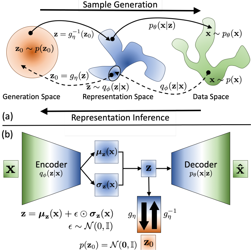
Figure 2: dpVAE: (a) The latent space is decoupled into a generation space with a simple, tractable distribution (e.g. standard normal) and a representation space whose distribution can be arbitrarily complex and is learned via a bijective mapping to the generation space. (b) Architecture of a VAE with the decoupled prior. The $g-$bijection is jointly trained with the VAE generative (i.e. decoder) and inference (i.e. encoder) models.

4 General Framework for VAE Regularization

In this section, we formally define and analyze how VAE regularizations affect the generative property of VAE. We also present the decoupled prior family for VAEs (see Figure 2) and analyze its utility to solve the submanifold problem of state-of-the-art regularization-based VAEs.

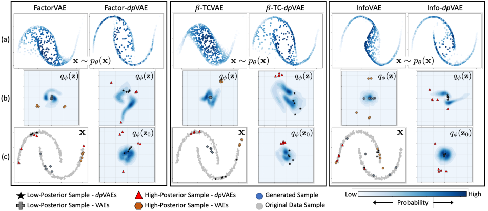
Figure 3: Sample generation and latent spaces for regularized VAEs: Each block is a VAE trained with a different regularizer on the two moons dataset, with and without the decoupled prior. In each block, (a) showcases the sample generation quality, (b) shows the aggregate posterior $q_{\phi}(\mathbf{z})$ with top five low- and high-posterior samples marked, and (c) shows the generation space for the decoupled prior and the training samples in the data space with corresponding low- and high-posterior samples are marked.

4.1 VAE Regularizers: Latent Pockets and Leaks

ELBO regularization is a conventional mechanism that enforces inductive biases (e.g. disentanglement [58, 20, 23, 37, 8, 28] and informative latent codes [35, 2]) to improve the representation learning aspect of VAEs [54]. These methods have shown their efficacy in learning good representations but neglect the generative property. Empirically, these regularizations improve the learned latent representation but inherently cause a mismatch between the aggregate posterior $q_{\phi}(\mathbf{z})=\mathbb{E}_{p(\mathbf{x})}\left[q_{\phi}(\mathbf{z}|\mathbf{x})\right]$ and the prior $p(\mathbf{z})$. This mismatch leads to latent pockets and leaks, or a submanifold in the aggregate posterior that results in poor generative capabilities. Specifically, if a sample $\mathbf{z}\sim p(\mathbf{z})$ (i.e. likely to be generated under the prior) lies in a pocket, (i.e. $q_{\phi}(\mathbf{z})$ is low), then its corresponding decoded sample $\mathbf{x}\sim p_{\theta}(\mathbf{x}|\mathbf{z})$ will not lie on the data manifold. This problem, caused by VAE regularizations, we call the submanifold problem.

To better understand this phenomena, we define two different types of samples in the VAE latent space that corresponds to two VAE failure modes.

Low-Posterior (LP) samples: These are samples that are highly likely to be generated under the prior (i.e. $p(\mathbf{z})$ is high) but are not covered by the aggregate posterior (i.e. $q_{\phi}(\mathbf{z})$ is low). The low-posterior samples are typically generated from the latent pockets dictated by the regularizer(s) used and are of poor quality since they lie off the data manifold. To generate low-posterior samples, we follow the logic of [47], where we sample $\mathbf{z}\sim p(\mathbf{z})=\mathcal{N}(\mathbf{z};\mathbf{0},\mathbb{I})$, rank them according to their aggregate posterior support, i.e. values of $q_{\phi}(\mathbf{z})$, and choose the samples with lowest aggregate posterior values. In the case of dpVAEs, samples are generated from $\mathbf{z}_{0}\sim p(\mathbf{z}_{0})=\mathcal{N}(\mathbf{z}_{0};\mathbf{0},\mathbb{I})$, which is a standard normal, and then transformed by $\mathbf{z}=g_{\eta}^{-1}(\mathbf{z}_{0})$ before plugging it into the aggregate posterior.

High-Posterior (HP) samples: These are samples supported under the aggregate posterior (i.e. $q_{\phi}(\mathbf{z})$ is high) but are less likely to be generated under the prior (i.e. $p(\mathbf{z})$ is low). Specifically, these are samples in the latent space that can produce good generated samples but are unlikely to be sampled due to the low support of the prior, and thereby they are samples that are in the latent leaks. To generate high-posterior samples, we sample from $\mathbf{z}\sim q_{\phi}(\mathbf{z})=\mathbb{E}_{p(\mathbf{x})}\left[q_{\phi}(\mathbf{z}|\mathbf{x})\right]$, rank them according to their prior support, i.e. values of $\mathcal{N}(\mathbf{z};\mathbf{0},\mathbb{I})$, and choose the samples with lowest prior support values. In the case of dpVAEs, sampled $\mathbf{z}$ are first mapped to the $\mathbf{z}_{0}-$space by $\mathbf{z}_{0}=g_{\eta}(\mathbf{z})$ before computing prior probabilities $\mathcal{N}(\mathbf{z}_{0};\mathbf{0},\mathbb{I})$.

In summary, a VAE performs well in the generative sense if the latent space is free of pockets and leaks. A pocket-free latent space is manifested by low-posterior samples that lie on the data manifold when mapped to the data space via the decoder $p_{\theta}(\mathbf{x}|\mathbf{z})$. In a leak-free latent space, high-posterior samples are supported by the aggregate posterior, yet with a tiny probability under the prior, and thereby these samples fall off the data manifold. This submanifold problem is demonstrated using four state-of-the-art VAE regularizers (see Figure 1 and Figure 3). With $\beta$-VAE [20], FactorVAE [23] and $\beta$-TCVAE [8], we can clearly see that the low-posterior samples lie in the latent pockets formed in the aggregate posterior (see Figure 3b) and they lie outside the data manifold (see Figure 3c), causing the sample generation to be very noisy (see Figure 3a). In the case of InfoVAE, the low-posterior samples lie in regions with not much aggregate posterior support causing a slightly noisy sample generation (see Figure 3a). More importantly, there are high-posterior samples that come from $q_{\phi}(\mathbf{z})$ but can very rarely be captured by a standard normal prior distribution. With the InfoVAE, for instance, the model fails to generate samples that lie on the tail-end of the top moon.

Although VAE regularizers improve latent representations, they sacrifice sample generation through the introduction of latent pockets and leaks. To fix sample generation, we propose a decoupling of the representation and generation spaces (see Figure 2a for illustration). This is demonstrated for $\beta$-VAE with and without decoupled prior in Figure 1, where the decoupled generation space $p(\mathbf{z}_{0})\sim\mathcal{N}(\mathbf{z}_{0};\mathbf{0},\mathbb{I})$ is used for generation and all the low-posterior samples lie on the data manifold. We formulate this prior in detail in following section.

4.2 dpVAE: Decoupled Prior for VAE

Decoupled prior family, as the name suggests, decouples the latent space that performs the representation and the space that drives sample generation. For this decoupling to be meaningful, the representation and generation spaces should be related by a functional mapping. The decoupled prior effectively learns the latent space distribution $p(\mathbf{z})$ by simultaneously learning the functional mapping $g_{\eta}$ together with the generative and inference models during optimization.

Specifically, the latent variables $\mathbf{z}\in\mathcal{Z}\subset\mathbb{R}^{L}$ and $\mathbf{z}_{0}\in\mathcal{Z}_{0}\subset\mathbb{R}^{L}$ are the random variables of the representation and generation spaces, respectively, where $p(\mathbf{z}_{0})\sim\mathcal{N}(\mathbf{z}_{0};\mathbf{0},\mathbb{I})$. The bijective mapping between the representation space $\mathcal{Z}$ and the generation space $\mathcal{Z}_{0}$ is defined by an invertible function $g_{\eta}(\mathbf{z})=\mathbf{z}_{0}$, parameterized by the network parameters $\eta$. VAE regularizers still act on the posteriors in the representation space, i.e. $q_{\phi}(\mathbf{z}|\mathbf{x})$ and/or $q_{\phi}(\mathbf{z})$, without affecting the latent distribution of the generation space $p(\mathbf{z}_{0})$. Sample generation starts by sampling $\mathbf{z}_{0}\sim p(\mathbf{z}_{0})$ , passing through the inverse mapping to obtain $\mathbf{z}=g_{\eta}^{-1}(\mathbf{z}_{0})$, which is then decoded by the generative model $p_{\theta}(\mathbf{x}|\mathbf{z})$ (see Figure 2a). These decoupled spaces can allow any modifications in the representation space dictated by the regularizer to infuse its submanifold structure in that space (see Figure 3b) without significantly impacting the generation space (see Figure 3c), and thereby improving sample generation for regularized VAEs (see Figure 3a). Moreover, the decoupled prior $p(\mathbf{z})$ is an expressive prior that is learned jointly with the VAE, and thereby it can match an arbitrarily complex aggregate posterior $q_{\phi}(\mathbf{z})$, thanks to the flexibility of deep networks to model complex mappings. Additionally, due to the bijective mapping $g_{\eta}$, we have a one-to-one correspondence between samples in $p(\mathbf{z}_{0})\sim\mathcal{N}(\mathbf{z}_{0};\mathbf{0},\mathbb{I})$ and those in $p(\mathbf{z})$.

To derive the ELBO for dpVAE, we replace the standard normal prior in (3.1) with the decoupled prior defined in (2). Using the change of variable formula, the KL divergence term in (3.1) can be simplified into:

$$\operatorname{KL}\left[q_{\phi}(\mathbf{z}|\mathbf{x})\|p(\mathbf{z})\right]=-\mathbb{E}_{q_{\phi}(\mathbf{z}|\mathbf{x})}\left[\sum_{k=1}^{K}\sum_{l=1}^{L}b_{k}^{l}s_{k}\left(b_{k}^{l}z_{k}^{l}\right)\right]$$

$$-\frac{1}{2}\log|\boldsymbol{\Sigma}_{\mathbf{z}}(\mathbf{x})|+\mathbb{E}_{q_{\phi}(\mathbf{z}|\mathbf{x})}\left[g_{\eta}(\mathbf{z})^{T}g_{\eta}(\mathbf{z})\right]$$ (5)

where $L$ is the latent dimension, $K$ is number of invertible blocks used to define the decoupled prior (see (9)), $s_{k}$ is the scaling network of the $k-$th block, $\boldsymbol{\Sigma}_{\mathbf{z}}(\mathbf{x})$ is the covariance matrix of the variational posterior $q_{\phi}(\mathbf{z}|\mathbf{x})$ (which is typically assumed to be diagonal), and $b_{k}^{l}$ and $z_{k}^{l}$ are the $l-$th element in $\mathbf{b}_{k}$ and $\mathbf{z}_{k}$ vectors, respectively.

4.3 dpVAE  in Concert with VAE Regularizers

The KL divergence in (5) can be directly used for any regularized ELBO. However, there are some regularized models such as $\beta$-TCVAE [8], and InfoVAE [58] that introduce additional terms other than $\operatorname{KL}\left[q_{\phi}(\mathbf{z}|\mathbf{x})\|p(\mathbf{z})\right]$ with $p(\mathbf{z})$. These regularizers need to be modified when used with decoupled priors.

$\beta$-dpVAE: For $\beta$-VAE (both $\beta$-VAE-H [20] and $\beta$-VAE-B [7] versions), the only difference in the ELBO (3.1) is reweighting the KL-term and the addition of certain constraints without introducing any additional terms. Hence, $\beta$-dpVAE  will retain the same reweighting and constraints, and only modify the KL divergence term according to (5).

Factor-dpVAE: FactorVAE [23] introduces a total correlation term $\operatorname{KL}\left[q_{\phi}(\mathbf{z})\|q_{\phi}(\bar{\mathbf{z}})\right]$ to the ELBO in (3.1), where $q_{\phi}(\bar{\mathbf{z}})=\prod_{l=1}^{L}q_{\phi}(z^{l})$ and $z^{l}$ is the $l-$th element of $\mathbf{z}$. This term promotes disentanglement of the latent dimensions of $\mathbf{z}$, impacting the representation learning aspect of VAE. Hence, in the case of the decoupled prior, the total correlation term should be applied to the representation space. In this sense, the decoupled prior only affects the KL divergence term as described in (5) for the Factor-dpVAE  model.

$\beta$-TC-dpVAE: Regularization provided by $\beta$-TCVAE [8] factorizes the ELBO into the individual latent dimensions based on the decomposition given in [22]. The only term that includes $p(\mathbf{z})$ is the KL divergence between marginals, i.e. $\operatorname{KL}\left[q_{\phi}(\mathbf{z})\|p(\mathbf{z})\right]$. This term in $\beta$-TCVAE is assumed to be factorized and is evaluated via sampling, facilitating the direct incorporation of the decoupled prior. In particular, we can just sample from the base distribution $\mathbf{z}_{0}\sim p(\mathbf{z}_{0})=\mathcal{N}(\mathbf{z}_{0};\mathbf{0},\mathbb{I})$ and compute the corresponding sample $\mathbf{z}\sim p(\mathbf{z})$ using $\mathbf{z}=g_{\eta}^{-1}(\mathbf{z}_{0})$.

Info-dpVAE: In InfoVAE [58], the additional term in the ELBO is again the divergence between aggregate posterior and the prior, i.e. $\operatorname{KL}\left[q_{\phi}(\mathbf{z})\|p(\mathbf{z})\right]$. This KL divergence term is replaced by different divergence families; adversarial training [36], Stein variational gradient [31], and maximum-mean discrepancy MMD [18, 30, 15]. However, adversarial-based divergences can have unstable training and Stein variational gradient scales poorly with high dimensions [58]. Motivated by the MMD-based results in [58], we focus here on the MMD divergence to evaluate this marginal divergence. For Info-dpVAE, we start with the ELBO of InfoVAE and modify the standard KL divergence term using (5). In addition, we compute the marginal KL divergence using MMD, which quantifies the divergence between two distributions by comparing their moments through sampling. Similar to $\beta$-TC-dpVAE, we can sample from $p(\mathbf{z}_{0})$ and use the inverse mapping to compute samples in the $\mathbf{z}-$space.

5 Experiments

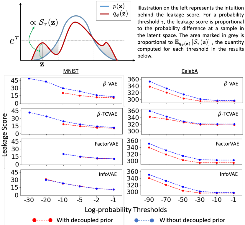
Figure 4: dpVAEs  have less latent leaks: Leakage scores for regularized VAEs on MNIST and CelebA data (missing values mean there are no samples with $\log(p(\mathbf{z}))<\tau$, implying zero leakage at that threshold).

Table 1: Generative metrics (lower is better) for vanilla VAE and regularized VAEs using standard normal and decoupled priors. FID = Fréchet Inception Distance. LP = Low-Posterior. sKL = symmetric KL divergence. NLL = Negative Log-Likelihood

Methods	MNIST				SVHN				CelebA
	FID	FID (LP)	sKL	NLL ($\times 10^{3}$)	FID	FID (LP)	sKL	NLL ($\times 10^{3}$)	FID	FID (LP)	sKL	NLL ($\times 10^{3}$)
VAE [24, 46]	137.4	165.0	1.26	3.56	78.9	83.8	53.67	0.386	81.4	79.0	59.3	9.26
dpVAE	129.0	153.1	0.88	3.53	50.8	55.2	13.02	0.318	71.5	74.3	10.4	4.91
$\beta$-VAE-H [20]	144.2	163.1	4.49	4.12	96.7	97.6	10.35	0.611	80.3	79.9	39.7	6.93
$\beta$-dpVAE-H	127.1	127.4	1.07	2.98	65.2	67.7	4.05	0.592	67.2	72.5	33.5	10.6
$\beta$-VAE-B [7]	130.8	163.6	2.74	3.11	61.7	68.5	2.62	0.606	75.7	79.6	25.8	12.5
$\beta$-dpVAE-B	113.3	114.1	1.32	2.80	51.1	50.3	2.47	0.550	67.9	72.0	19.1	10.4
$\beta$-TCVAE [8]	149.8	200.3	4.48	2.91	69.2	70.5	7.76	9.86	83.8	83.0	93.6	9.33
$\beta$-TC-dpVAE	133.3	133.1	2.07	2.70	50.3	53.8	2.94	4.52	80.3	81.4	90.3	10.0
FactorVAE [23]	130.5	191.2	1.04	3.50	97.2	108.5	1.91	2.13	82.6	86.8	71.3	9.89
Factor-dpVAE	120.8	121.3	0.85	3.60	86.3	86.9	1.57	2.36	65.0	73.4	51.3	12.2
InfoVAE [58]	128.7	133.2	2.89	2.88	81.3	83.2	4.91	1.55	76.5	79.1	30.6	11.1
Info-dpVAE	110.1	110.5	1.70	2.81	62.9	67.7	2.67	1.56	68.9	72.9	20.3	12.1

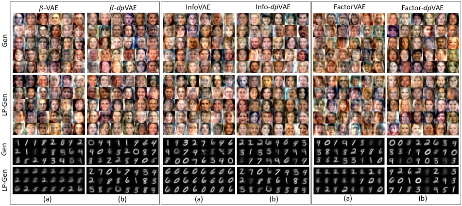
Figure 5: dpVAEs  generate low-posterior samples with better quality: We show generated (Gen) and low-posterior (LP-Gen) samples for CelebA and MNIST on regularized VAEs (a) without and (b) with decoupled priors.

We experiment with three benchmark image datasets, namely MNIST [29], SVHN [40], CelebA (cropped version) [32]. We train these datasets with VAE [24, 46] and five regularized VAEs, namely $\beta$-VAE-H [20], $\beta$-VAE-B [7], $\beta$-TCVAE) [8], FactorVAE [23] and InfoVAE [58]. We showcase, qualitatively and quantitatively, that dpVAEs  improve sample generation while retaining the benefits of representation learning provided by the regularizers.

5.1 Generative Metrics

We use the following quantitative metrics to assess the generative performance of the regularized VAEs with the decoupled prior in contrast to the standard normal prior.

Fréchet Inception Distance (FID): The FID score is based on the statistics, assuming Gaussian distribution, computed in the feature space defined using the inception network features [52]. FID score quantifies both the sample diversity and quality. Lower FID means better sample generation.

Symmetric KL Divergence (sKL): To quantify the overlap between $p(\mathbf{z})$ and $q_{\phi}(\mathbf{z})$ in the representation space ($p(\mathbf{z})$ being the decoupled prior for dpVAEs  or the standard normal), we compute $\operatorname{sKL}\!\!\!=\operatorname{KL}\left[p(\mathbf{z})\|q_{\phi}(\mathbf{z})\right]+\operatorname{KL}\left[q_{\phi}(\mathbf{z})\|p(\mathbf{z})\right]$ through sampling (using 5,000 samples). sKL also captures the existence of pockets and leaks in $q_{\phi}(\mathbf{z})$. Lower sKL implies there is a better overlap between $p(\mathbf{z})$ and $q_{\phi}(\mathbf{z})$, indicating better generative capabilities.

Negative Log-likelihood: We estimate the likelihood of held-out samples under a trained model using importance sampling (with 21,000 samples) proposed in [46], where $\operatorname{NLL}\!\!\!=\!\!\!\log\mathbb{E}_{q_{\phi}(\mathbf{z}|\mathbf{x})}\left[p_{\theta}(\mathbf{x}|\mathbf{z})p(\mathbf{z})/q_{\phi}(\mathbf{z}|\mathbf{x})\right]$. Lower NLL means better sample generation since the learned model supports unseen samples drawn from the data distribution.

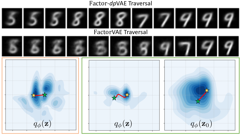
Figure 6: Latent traversal for dpVAEs  does not path through latent pockets: The top rows showcases latent traversal for FactorVAE and Factor-dpVAE  on MNIST data. The orange box is the $q_{\phi}(\mathbf{z})$ for FactorVAE and the red line shows the traversal between starting and ending points (green and yellow stars, respectively). The green box shows the same traversal in $q_{\phi}(\mathbf{z}_{0})$ that is mapped using $g_{\eta}^{-1}$ to the representation space, demonstrated using $q_{\phi}(\mathbf{z})$. We see that the traversal path in $q_{\phi}(\mathbf{z})$ tries to avoid low probability regions, which correspond to better image quality.

Leakage Score: To assess the effect of decoupled priors on latent leaks (as manifested by high posterior samples), we devise a new metric based on log-probability differences. We sample from the aggregate posterior $\mathbf{z}\sim q_{\phi}(\mathbf{z})$. If $\log(p(\mathbf{z}))<\tau$, where $\tau\in\mathbb{R}$ is a chosen threshold value, then we consider the sample to lie in a “leakage region” defined by $\tau$. This sample is considered a high-posterior sample at the $\tau-$level since the sample is better supported under the aggregate posterior than the prior (see illustration in Figure 4). Based on the threshold value, these leakage regions are less likely to be sampled from. In order to not lose significant regions from the data manifold, we want the aggregate posterior corresponding to these samples to attain low values as well. To quantify latent leakage for a trained model, we propose a leakage score as $\operatorname{LS}(\tau)=\mathbb{E}_{q_{\phi}(\mathbf{z})}\left[\mathcal{S}_{\tau}(\mathbf{z})\right]$, where for a given $\mathbf{z}\sim q_{\phi}(\mathbf{z})$ at a particular threshold $\tau$, $\mathcal{S}_{\tau}(\mathbf{z})$ is defined as:

$$\mathcal{S}_{\tau}(\mathbf{z})=\begin{cases}\log\left(\frac{q_{\phi}(\mathbf{z})}{p(h(\mathbf{z}))}\right)&\log(p(\mathbf{z}))<\tau\\ 0&\log(p(\mathbf{z}))\geq\tau\end{cases}$$ (6)

Here, $h$ is the identity function in VAEs with standard normal prior, and is $g_{\eta}$ for dpVAEs.

5.2 Generation Results and Analysis

In Table 1, we observe that dpVAEs  perform better than their corresponding regularized VAEs without the decoupled prior for each dataset. When comparing VAEs with and without decoupled priors (e.g. InfoVAE and Info-dpVAE), we use the same hyperparameters and perform no additional tuning. This showcases the robustness of the decoupled prior w.r.t. hyperparameters, facilitating its direct use with any regularized VAE. We report the FID scores on both the randomly generated samples from the prior and the low-posterior samples. As analyzed in section 4.1, if the low-posterior samples lie on the data manifold, then the learned latent space is pocket-free. Results in Table 1 suggest that for all dpVAEs, the FID scores for the randomly generated samples and low-posterior ones are comparable, suggesting that all the pockets in the latent space are filled. Qualitative results of sample generation for CelebA and MNIST are shown in Figure 5. We show both the random prior and low-posterior sample generation with and without the decoupled prior for three different regularizations. The quality of generated samples using dpVAEs  is better or on par with those without the decoupled prior. But more importantly, one can observe a significant quality improvement in the low-posterior samples, which aligns with the quantitative results in Table 1. In Figure 4, we report the leakage score $\operatorname{LS}(\tau)$ as a function of log-probability thresholds for different regularizers with and without the decoupled priors. We observe that dpVAEs  result in models with lower latent leakage. This is especially true at lower thresholds, which suggests that even when $p(\mathbf{z})$ is small, the $q_{\phi}(\mathbf{z})$ is small as well, preventing the loss of significant regions from the data manifold.

5.3 Latent Traversals Results

We perform latent traversals between samples in the latent space. We expect that in VAEs, there will be instances of the traversal path crossing the latent pockets resulting in poor intermediate samples. In contrast, we expect dpVAEs  will map the linear traversal in $\mathbf{z}_{0}$ (generation space) to a non-linear traversal in $\mathbf{z}$ (representation space), while avoiding low probability regions. This is observed for MNIST data traversal ($L=2$) and is depicted in Figure 6.

We also qualitatively observe similar occurrences in CelabA traversals (see Figure 7). Finally, we want to attest that the addition of the decoupled prior to a regularizer does not affect it’s ability to improve the latent representation. We demonstrate this by observing latent factor traversals for CelebA trained on Factor-dpVAE, where we vary one dimension of the latent space while fixing the others. One can observe that Factor-dpVAE  is able to isolate different attributes of variation in the data, as shown in Figure 8.

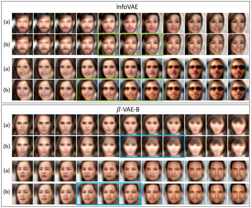
Figure 7: Latent traversals on CelebA: (a) with and (b) without decoupled prior. We notice for InfoVAE, the green boxes highlight the faces with unrealistic deformations, such as excessive teeth in the second row and noisy images in the fourth row. In comparison, Info-dpVAE  results in a more smooth traversal. We see similar effects from $\beta$-VAE, with odd shadowing due to hair and face rotation, highlighted in blue boxes. Again, $\beta$-dpVAE  makes these transitions smooth and seamless.

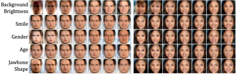
Figure 8: Factor-dpVAE  latent traversals across the top five latent dimensions sorted by their standard deviation from $q_{\phi}(\mathbf{z})$: Traversals start with the reconstructed image of a given sample and move $\pm 5$ standard deviations along a latent dimension. Results from other dpVAEs  similarly retain the latent space disentanglement.

6 Conclusion

In this paper, we define and analyze the submanifold problem for regularized VAEs, or the tendency of a regularizer to accentuate the creation of pockets and leaks in the latent space. This submanifold structure manifests the mismatch between the aggregate posterior and the latent prior which in turn causes degradation in generation quality. To overcome this trade-off between sample generation and latent representation, we propose the decoupled prior family as a general regularization framework for VAE and demonstrate its efficacy on state-of-the-art VAE regularizers. We demonstrate that dpVAEs  generate better quality samples as compared with their standard normal prior based counterparts, via qualitative and quantitative results. Additionally, we qualitatively observe that the representation learning (as improved by the regularizer) is not adversely affected by dpVAEs. Decoupled priors can act as a pathway to realizing the true potential of VAEs as both a representation learning and a generative modeling framework. Further work in this direction will include exploring more expressive inference and generative models (e.g. PixelCNN [55]) in conjuction with decoupled priors. We also believe more sophisticated invertible architectures (e.g. RAD [14]) and base distributions will provide further improvements.

Appendix

This appendix includes the derivation of dpVAE  training objective, the ELBO definitions of state-of-the-art VAE regularizers with the decoupled prior, and experimental details (architecture, hyperparameters, and train/test splits) for MNIST, SVHN and CelebA experiments.

Appendix A Derivation of $\operatorname{KL}\left[q_{\phi}(\mathbf{z}|\mathbf{x})\|p(\mathbf{z})\right]$ with Decoupled Prior

Consider a bijective mapping between $\mathcal{Z}$ and $\mathcal{Z}_{0}$ defined by a function $g_{\eta}(\mathbf{z})=\mathbf{z}_{0}$. The change of variable formula for mapping probability distribution on $\mathbf{z}$ to $\mathbf{z}_{0}$ is given as follows:

$$p(\mathbf{z})=p(\mathbf{z}_{0})\bigg{|}\frac{\partial\mathbf{z}_{0}}{\partial\mathbf{z}}\bigg{|}=p(g_{\eta}(\mathbf{z}))\bigg{|}\frac{\partial g_{\eta}(\mathbf{z})}{\partial\mathbf{z}}\bigg{|}$$ (7)

The $g-$bijection is parameterized by $K$ affine coupling layers, each layer is a bijection block $\mathbf{z}_{k-1}=g_{\eta}^{(k)}(\mathbf{z}_{k})$ of the form,

$$g_{\eta}^{(k)}(\mathbf{z}_{k}) = \mathbf{b}_{k}\odot\mathbf{z}_{k}$$ (8)

$$+ (1-\mathbf{b}_{k})\odot\left[\mathbf{z}_{k}\odot\exp\left(s_{k}(\mathbf{b}_{k}\odot\mathbf{z}_{k})\right)\right.$$

$$~{}~{}~{}~{}~{}~{}~{}~{}~{}~{}~{}~{}~{}~{}~{}~{}~{}~{}~{}\left.+t_{k}\left(\mathbf{b}_{k}\odot\mathbf{z}_{k}\right)\right],$$

where $\mathbf{z}=\mathbf{z}_{K}$, $\odot$ is the Hadamard (i.e. element-wise) product, $\mathbf{b}_{k}\in\{0,1\}^{L}$ is a binary mask used for partitioning the $k-$th block input, and $\eta=\{s_{1},...,s_{K},t_{1},...,t_{K}\}$ are the deep networks parameters of the scaling $s_{k}$ and translation $t_{k}$ functions of the $K$ blocks. Stacking these affine coupling layers constitutes the functional mapping between the representation and the generation spaces. The $g-$bijection is thus defined as,

$$g_{\eta}(\mathbf{z})=\mathbf{z}_{0}=g_{\eta}^{(1)}\circ\dots\circ g_{\eta}^{(K-1)}\circ g_{\eta}^{(K)}(\mathbf{z}).$$ (9)

The KL divergence is given as,

$$\operatorname{KL} := \operatorname{KL}\left[q_{\phi}(\mathbf{z}|\mathbf{x})\|p(\mathbf{z})\right]$$ (10)

$$= \int q_{\phi}(\mathbf{z}|\mathbf{x})\left[\log(q_{\phi}(\mathbf{z}|\mathbf{x}))-\log(p(\mathbf{z}))\right]d\mathbf{z}.$$

Using the change of variable formula in (7), we have the following.

$$\operatorname{KL} = \int q_{\phi}(\mathbf{z}|\mathbf{x})\bigg{[}\log(q_{\phi}(\mathbf{z}|\mathbf{x}))-\log(p(g_{\eta}(\mathbf{z})))$$ (12)

$$~{}~{}~{}~{}~{}~{}~{}~{}~{}~{}~{}~{}~{}-\log\left(\bigg{|}\frac{\partial g_{\eta}(\mathbf{z})}{\partial\mathbf{z}}\bigg{|}\right)\bigg{]}d\mathbf{z}$$

$$= \operatorname{KL}\left[q_{\phi}(\mathbf{z}|\mathbf{x})\|p(g_{\eta}(\mathbf{z}))\right]$$

$$~{}~{}~{}~{}~{}~{}~{}~{}~{}~{}~{}~{}~{}-\mathbb{E}_{q_{\phi}(\mathbf{z}|\mathbf{x})}\left[\log\left(\bigg{|}\frac{\partial g_{\eta}(\mathbf{z})}{\partial\mathbf{z}}\bigg{|}\right)\right].$$

The first term in (12) can be derived as follows,

$$T_{1} =\operatorname{KL}\left[q_{\phi}(\mathbf{z}|\mathbf{x})\|p(g_{\eta}(\mathbf{z}))\right]$$ (13)

$$=\int q_{\phi}(\mathbf{z}|\mathbf{x})\log\left(\frac{q_{\phi}(\mathbf{z}|\mathbf{x})}{p(g_{\eta}(\mathbf{z}))}\right)d\mathbf{z}$$ (14)

$$=-\mathbb{H}(q_{\phi}(\mathbf{z}|\mathbf{x}))-\int q_{\phi}(\mathbf{z}|\mathbf{x})\log\left(p(g_{\eta}(\mathbf{z})\right)d\mathbf{z},$$ (15)

where $\mathbb{H}(q_{\phi}(\mathbf{z}|\mathbf{x}))$ is the differential entropy of the variational posterior distribution. This approximate posterior is a multivariate Gaussian with a diagonal covariance matrix, i.e. $q_{\phi}(\mathbf{z}|\mathbf{x})\sim\mathcal{N}(\mathbf{z};\boldsymbol{\mu}_{\mathbf{z}}(\mathbf{x}),\boldsymbol{\Sigma}_{\mathbf{z}}(\mathbf{x}))$, where $\boldsymbol{\Sigma}_{\mathbf{z}}(\mathbf{x})=\operatorname{diag}(\boldsymbol{\sigma}_{\mathbf{z}}(\mathbf{x}))$, and $\boldsymbol{\sigma}_{\mathbf{z}}(\mathbf{x})\in\mathbb{R}^{L}_{+}$. This results in a closed-form expression for the entropy of the approximate posterior [42], given as:

$$\mathbb{H}(q_{\phi}(\mathbf{z}|\mathbf{x}))=\frac{L}{2}+\frac{L}{2}\log(2\pi)+\frac{\log|\boldsymbol{\Sigma}_{\mathbf{z}}(\mathbf{x})|}{2}.$$ (16)

The probability of the base latent space (i.e. the generation space) in the decoupled prior is assumed to be a standard normal distribution, i.e. $p(g_{\eta}(\mathbf{z}))=\mathcal{N}(g_{\eta}(\mathbf{z});0,\mathbb{I}_{L})$. Together with (16) and ignoring constants terms, the first term in (12) can be simplified into,

$$T_{1} = -\frac{\log|\boldsymbol{\Sigma}_{\mathbf{z}}(\mathbf{x})|}{2}+\int q_{\phi}(\mathbf{z}|\mathbf{x})\frac{L}{2}\log\left(\frac{1}{2\pi}\right)d\mathbf{z}$$

$$+ \frac{1}{2}\int q_{\phi}(\mathbf{z}|\mathbf{x})g_{\eta}(\mathbf{z})^{T}g_{\eta}(\mathbf{z})d\mathbf{z}$$

$$= \frac{1}{2}\bigg{[}-\log{|\boldsymbol{\Sigma}_{\mathbf{z}}(\mathbf{x})|}+const$$

$$+ \mathbb{E}_{q(\mathbf{z}|\mathbf{x})}\left[g_{\eta}(\mathbf{z})^{T}g_{\eta}(\mathbf{z})\right]\bigg{]}$$ (18)

The second term in (12) can be derived as follows,

$$T_{2} = \mathbb{E}_{q_{\phi}(\mathbf{z}|\mathbf{x})}\left[\log{\left(\bigg{|}\frac{\partial g_{\eta}(\mathbf{z})}{\partial\mathbf{z}}\bigg{|}\right)}\right]$$ (19)

$$= \int q_{\phi}(\mathbf{z}|\mathbf{x})\log{\left(\bigg{|}\frac{\partial g_{\eta}(\mathbf{z})}{\partial\mathbf{z}}\bigg{|}\right)}d\mathbf{z}.$$

Applying the chain rule to $g_{\eta}(\mathbf{z})$, which is a composition of functions as defined in (9), and combining this with the multiplicative property of determinants, we have the following,

$$\bigg{|}\frac{\partial g_{\eta}(\mathbf{z})}{\partial\mathbf{z}}\bigg{|}=\prod\limits_{k=1}^{K}\bigg{|}\frac{\partial g_{\eta}^{(k)}(\mathbf{z}_{k})}{\partial\mathbf{z}_{k}}\bigg{|}.$$ (20)

Hence, we have the second term in (12) can be expressed as follows:

$$T_{2} =\mathbb{E}_{q_{\phi}(\mathbf{z}|\mathbf{x})}\left[\sum\limits_{k=1}^{K}\log{\left(\bigg{|}\frac{\partial g_{\eta}^{(k)}(\mathbf{z}_{k})}{\partial\mathbf{z}_{k}}\bigg{|}\right)}\right].$$ (21)

Similar to [13], deriving the Jacobian of individual affine coupling layers yields to an upper triangular matrix. Hence, the determinant is simply the product of the diagonal values, resulting in,

$$\log\left(\bigg{|}\frac{\partial g_{\eta}^{(k)}(\mathbf{z}_{k})}{\partial\mathbf{z}_{k}}\bigg{|}\right)=\sum\limits_{l=1}^{L}b^{l}_{k}s_{k}(b^{l}_{k}z^{l}_{k}).$$ (22)

Using this simplification, we finally have an expression for the second term expressed as,

$$T_{2}=\mathbb{E}_{q_{\phi}(\mathbf{z}|\mathbf{x})}\left[\sum\limits_{k=1}^{K}\sum\limits_{l=1}^{L}b^{l}_{k}s_{k}(b^{l}_{k}z^{l}_{k})\right].$$ (23)

Substituting (23) and (18) in (12), the KL divergence term of the decoupled prior can be written as,

$$\operatorname{KL} = \frac{1}{2}\bigg{[}-\log{|\boldsymbol{\Sigma}_{\mathbf{z}}(\mathbf{x})|}+\mathbb{E}_{q(\mathbf{z}|\mathbf{x})}\left[g_{\eta}(\mathbf{z})^{T}g_{\eta}(\mathbf{z})\right]\bigg{]}$$ (24)

$$- \mathbb{E}_{q_{\phi}(\mathbf{z}|\mathbf{x})}\left[\sum\limits_{k=1}^{K}\sum\limits_{l=1}^{L}b^{l}_{k}s_{k}(b^{l}_{k}z^{l}_{k})\right]$$

Appendix B ELBOs for Different Regularizers

In this section, we define the ELBO (i.e. training objective) for individual regularizers considered (see section 4.3 in the main manuscript) and how they differ under the application of decoupled prior. Here, we only serve to provide more mathematical clarity of these modifications.

$\beta$-dpVAE: The ELBO for the $\beta$-VAE [20] can be expressed as follows:

$$\mathcal{L}(\theta,\phi) =\mathbb{E}_{p(\mathbf{x})}[\mathbb{E}_{q_{\phi}(\mathbf{z}|\mathbf{x})}\left[\log p_{\theta}(\mathbf{x}|\mathbf{z})\right]$$

$$-\beta\operatorname{KL}\left[q_{\phi}(\mathbf{z}|\mathbf{x})\|p(\mathbf{z})\right]]$$ (25)

By substituting the KL divergence under the decoupled prior, the ELBO for $\beta$-dpVAE  can defined as follows:

$$\mathcal{L}(\theta,\phi,\eta) =\mathbb{E}_{p(\mathbf{x})}[\mathbb{E}_{q_{\phi}(\mathbf{z}|\mathbf{x})}\left[\log p_{\theta}(\mathbf{x}|\mathbf{z})\right]$$

$$-\frac{\beta}{2}\big{[}-\log{|\boldsymbol{\Sigma}_{\mathbf{z}}(\mathbf{x})|}+\mathbb{E}_{q(\mathbf{z}|\mathbf{x})}\left[g_{\eta}(\mathbf{z})^{T}g_{\eta}(\mathbf{z})\right]\big{]}$$

$$-\beta\mathbb{E}_{q_{\phi}(\mathbf{z}|\mathbf{x})}\left[\sum\limits_{k=1}^{K}\sum\limits_{l=1}^{L}b^{l}_{k}s_{k}(b^{l}_{k}z^{l}_{k})\right]]$$ (26)

The alternate formulation, $\beta$-VAE-B [7], has a similar ELBO function with some additional parameters applied to the KL divergence term.

Factor-dpVAE: The ELBO for FactorVAE [23] is given as follows:

$$\mathcal{L}(\theta,\phi) =\mathbb{E}_{p(\mathbf{x})}[\mathbb{E}_{q_{\phi}(\mathbf{z}|\mathbf{x})}\left[\log p_{\theta}(\mathbf{x}|\mathbf{z})\right]$$

$$-\operatorname{KL}\left[q_{\phi}(\mathbf{z}|\mathbf{x})\|p(\mathbf{z})\right]]-\gamma\operatorname{KL}\left[q_{\phi}(\mathbf{z})\|q_{\phi}(\bar{\mathbf{z}})\right]$$ (27)

To modifying this ELBO with the decoupled prior, the KL divergence term between the posterior and prior that contains $p(\mathbf{z})$ is the only term that needs to be reformulated. This results in:

$$\mathcal{L}(\theta,\phi,\eta) =\mathbb{E}_{p(\mathbf{x})}[\mathbb{E}_{q_{\phi}(\mathbf{z}|\mathbf{x})}\left[\log p_{\theta}(\mathbf{x}|\mathbf{z})\right]$$

$$-\frac{1}{2}[-\log{(|\boldsymbol{\Sigma}_{\mathbf{z}}(\mathbf{x})|)}+\mathbb{E}_{q(\mathbf{z}|\mathbf{x})}\left[g_{\eta}(\mathbf{z})^{T}g_{\eta}(\mathbf{z})\right]]$$

$$-\mathbb{E}_{q_{\phi}(\mathbf{z}|\mathbf{x})}\left[\sum\limits_{k=1}^{K}\sum\limits_{l=1}^{L}b^{l}_{k}s_{k}(b^{l}_{k}z^{l}_{k})\right]]$$ (28)

$$-\gamma\operatorname{KL}\left[q_{\phi}(\mathbf{z})\|\bar{q_{\phi}(\mathbf{z})}\right]$$ (29)

$\beta$-TC-dpVAE: Following similar notation as provided in [8], the ELBO for $\beta$-TCVAE [8] is given as follows:

$$\mathcal{L}(\theta,\phi) =\mathbb{E}_{p(n)}\left[\mathbb{E}_{q_{\phi}(\mathbf{z}|n)}\left[\log p_{\theta}(n|\mathbf{z})\right]\right]$$

$$-\alpha I_{q_{\phi}}(\mathbf{z};n)-\beta\operatorname{KL}\left[q_{\phi}(\mathbf{z})\|\prod\limits_{j}q_{\phi}(z_{j})\right]$$

$$-\gamma\sum\limits_{j}\operatorname{KL}\left[q_{\phi}(z_{j})\|p(z_{j})\right]$$ (30)

Due to the factorized representation of the prior, the last KL divergence is computed via sampling. Hence, the modification for the decoupled prior becomes trivial. We simply sample from $\mathbf{z}_{0}$ space (which is assumed to be factorized) and pass it through $g_{\eta}^{-1}(z_{0j})$ to obtain a sample in $\mathbf{z}$ space, the ELBO can thus be modified as follows:

$$\mathcal{L}(\theta,\phi,\eta) =\mathbb{E}_{p(n)}\left[\mathbb{E}_{q_{\phi}(\mathbf{z}|n)}\left[\log p_{\theta}(n|\mathbf{z})\right]\right]$$

$$-\alpha I_{q_{\phi}}(\mathbf{z};n)-\beta\operatorname{KL}\left[q_{\phi}(\mathbf{z})\|\prod\limits_{j}q_{\phi}(z_{j})\right]$$

$$-\gamma\sum\limits_{j}\operatorname{KL}\left[q_{\phi}(z_{j})\|p(g_{\eta}^{-1}(z_{0j}))\right]$$ (31)

Info-dpVAE: For InfoVAE [58], the ELBO (using the MMD divergence) is given as follows:

$$\mathcal{L}(\theta,\phi) =\mathbb{E}_{p(\mathbf{x})}[\mathbb{E}_{q_{\phi}(\mathbf{z}|\mathbf{x})}\left[\log p_{\theta}(\mathbf{x}|\mathbf{z})\right]$$

$$-(1-\alpha)\operatorname{KL}\left[q_{\phi}(\mathbf{z}|\mathbf{x})\|p(\mathbf{z})\right]]$$

$$-(\alpha+\lambda-1)D_{MMD}(q_{\phi}(\mathbf{z})||p(\mathbf{z}))$$ (32)

The modification for the decoupled prior takes place in two terms; the MMD divergence term, which is computed via sampling from the aggregate posterior, and the prior in $\mathbf{z}$ space, which acts on the representation space in the decoupled prior. Therefore, the modification is very similar to the one applied in $\beta$-TCVAE. Additionally, the KL divergence term will be modified normally. The final ELBO is thus as follows:

$$\mathcal{L}(\theta,\phi,\eta) =\mathbb{E}_{p(\mathbf{x})}[\mathbb{E}_{q_{\phi}(\mathbf{z}|\mathbf{x})}\left[\log p_{\theta}(\mathbf{x}|\mathbf{z})\right]$$

$$-\frac{1-\alpha}{2}[-\log{(|\boldsymbol{\Sigma}_{\mathbf{z}}(\mathbf{x})|)}+\mathbb{E}_{q(\mathbf{z}|\mathbf{x})}\left[g_{\eta}(\mathbf{z})^{T}g_{\eta}(\mathbf{z})\right]]$$

$$-(1-\alpha)\mathbb{E}_{q_{\phi}(\mathbf{z}|\mathbf{x})}\left[\sum\limits_{k=1}^{K}\sum\limits_{l=1}^{L}b^{l}_{k}s_{k}(b^{l}_{k}z^{l}_{k})\right]]$$

$$-D_{MMD}(q_{\phi}(\mathbf{z})||p(g_{\eta}^{-1}(\mathbf{z}_{0})))$$ (33)

Appendix C Architectures and Hyperparameters

In this section, we give more details for the architecture and hyperparameters used and the data handling for the four different datasets used in the paper, namely two moons toy data, MNIST, SVHN, and CelebA. These are also described for different regularizers used on each of these datasets.

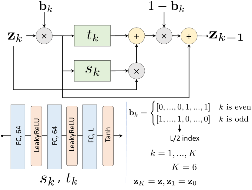
Figure 9: Architecture details of the decoupled prior. Architecture description of individual affine coupling blocks and the details of binary masks. The top shows the structure of an individual affine coupling layer representing the function $g_{\eta}^{(k)}(\mathbf{z}_{k})$. Sndividual scaling $s_{k}$ and translation $t_{k}$ functions have the same architecture for all the block (bottom-left). Bottom-right shows the binary masks and number of affine coupling layers.

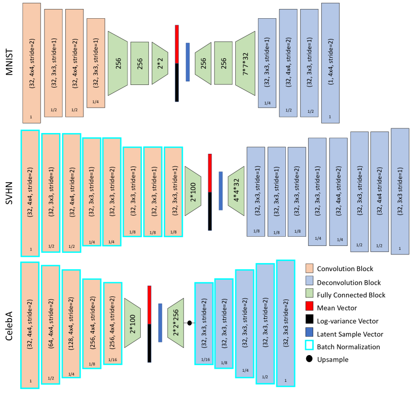
Figure 10: Architecture description for different datasets. This figure shows the VAE architecture for MNIST, SVHN, and CelebA datasets. This architecture is kept the same for all the regularizations with and without the decoupled prior.

Figure 10 illustrates the VAE architecture for all the datasets and the regularizers reported in the experiments section of the paper. For MNIST and SVHN, we use ReLU as the non-linear activation function, and for CelebA we use leaky ReLU [34]. For the two moons data, the VAE architecture consists of two fully connected layers of size 100 and 50 (from input to latent space) in the encoder. The decoder is a mirrored version of the encoder.We use two-dimensional latent space for the two moons data. The architecture that is added for the decoupled prior is the same for all the experiments we present in the paper. This architecture for the affine coupling layers that connects $\mathbf{z}$ and $\mathbf{z}_{0}$ is shown in Figure 9.

FactorVAE [23] has a discriminator architecture, which has five fully connected layers each with 1000 hidden units. Each fully connected layer is followed by a leaky ReLU activation of negative slope of 0.2. This discriminator architecture is the same for all experiments, except for the changing input size (i.e. the latent dimension $L$).

The learning rate for all the experiments was set to be $10^{-4}$, and the batch size for MNIST was 100, SVHN and CelebA were 50. We execute all the experiments for 100,000 iterations (100,000/B epochs where B is the batch size). No other pre-processing was performed while conducting these experiments. The regularization specific hyperparameters are mentioned in Table 2. These hyperparameters were kept the same for all datasets.

Table 2: Table representing hyperparameters for individual regularizations. These hyperparameters were set to be the same with and without the decoupled prior.

Methods	Parameters
$\beta$-VAE-H [20]	$\beta=4$
$\beta$-VAE-B [7]	$\gamma=15$, $C_{max}=25$, $C_{stop}=100000$
$\beta$-TC-VAE [8]	$\alpha=1$, $\beta=4$, $\gamma=15$
FactorVAE [23]	$\gamma=1000$
InfoVAE [58]	$\alpha=0$, $\lambda=1000$

References

- [1] Alexander Alemi, Ben Poole, Ian Fischer, Joshua Dillon, Rif A Saurous, and Kevin Murphy. Fixing a broken elbo. In International Conference on Machine Learning, pages 159–168, 2018.
- [2] Alexander A Alemi, Ian Fischer, Joshua V Dillon, and Kevin Murphy. Deep variational information bottleneck. ICLR, 2016.
- [3] Martin Arjovsky, Soumith Chintala, and Léon Bottou. Wasserstein generative adversarial networks. In International conference on machine learning, pages 214–223, 2017.
- [4] Matthias Bauer and Andriy Mnih. Resampled priors for variational autoencoders. In The 22nd International Conference on Artificial Intelligence and Statistics, pages 66–75, 2019.
- [5] Yoshua Bengio, Aaron Courville, and Pascal Vincent. Representation learning: A review and new perspectives. IEEE transactions on pattern analysis and machine intelligence, 35(8):1798–1828, 2013.
- [6] Samuel R Bowman, Luke Vilnis, Oriol Vinyals, Andrew Dai, Rafal Jozefowicz, and Samy Bengio. Generating sentences from a continuous space. In Proceedings of The 20th SIGNLL Conference on Computational Natural Language Learning, pages 10–21, 2016.
- [7] Christopher P Burgess, Irina Higgins, Arka Pal, Loic Matthey, Nick Watters, Guillaume Desjardins, and Alexander Lerchner. Understanding disentangling in beta-vae. arXiv preprint arXiv:1804.03599, 2018.
- [8] Tian Qi Chen, Xuechen Li, Roger B Grosse, and David K Duvenaud. Isolating sources of disentanglement in variational autoencoders. In Advances in Neural Information Processing Systems, pages 2610–2620, 2018.
- [9] Xi Chen, Yan Duan, Rein Houthooft, John Schulman, Ilya Sutskever, and Pieter Abbeel. Infogan: Interpretable representation learning by information maximizing generative adversarial nets. In Advances in neural information processing systems, pages 2172–2180, 2016.
- [10] Xi Chen, Diederik P Kingma, Tim Salimans, Yan Duan, Prafulla Dhariwal, John Schulman, Ilya Sutskever, and Pieter Abbeel. Variational lossy autoencoder. ICLR, 2017.
- [11] Nat Dilokthanakul, Pedro AM Mediano, Marta Garnelo, Matthew CH Lee, Hugh Salimbeni, Kai Arulkumaran, and Murray Shanahan. Deep unsupervised clustering with gaussian mixture variational autoencoders. arXiv preprint arXiv:1611.02648, 2016.
- [12] Laurent Dinh, David Krueger, and Yoshua Bengio. Nice: Non-linear independent components estimation, 2014.
- [13] Laurent Dinh, Jascha Sohl-Dickstein, and Samy Bengio. Density estimation using real nvp. ICLR, 2017.
- [14] Laurent Dinh, Jascha Sohl-Dickstein, Razvan Pascanu, and Hugo Larochelle. A RAD approach to deep mixture models. CoRR, abs/1903.07714, 2019.
- [15] Gintare Karolina Dziugaite, Daniel M Roy, and Zoubin Ghahramani. Training generative neural networks via maximum mean discrepancy optimization. In Proceedings of the Thirty-First Conference on Uncertainty in Artificial Intelligence, pages 258–267. AUAI Press, 2015.
- [16] Ian Goodfellow, Jean Pouget-Abadie, Mehdi Mirza, Bing Xu, David Warde-Farley, Sherjil Ozair, Aaron Courville, and Yoshua Bengio. Generative adversarial nets. In Advances in neural information processing systems, pages 2672–2680, 2014.
- [17] Karol Gregor, Ivo Danihelka, Alex Graves, Danilo Rezende, and Daan Wierstra. Draw: A recurrent neural network for image generation. In International Conference on Machine Learning, pages 1462–1471, 2015.
- [18] Arthur Gretton, Karsten Borgwardt, Malte Rasch, Bernhard Schölkopf, and Alex J Smola. A kernel method for the two-sample-problem. In Advances in neural information processing systems, pages 513–520, 2007.
- [19] Ishaan Gulrajani, Kundan Kumar, Faruk Ahmed, Adrien Ali Taiga, Francesco Visin, David Vazquez, and Aaron Courville. Pixelvae: A latent variable model for natural images. ICLR, 2017.
- [20] Irina Higgins, Loic Matthey, Arka Pal, Christopher Burgess, Xavier Glorot, Matthew Botvinick, Shakir Mohamed, and Alexander Lerchner. beta-vae: Learning basic visual concepts with a constrained variational framework. ICLR, 2(5):6, 2017.
- [21] Irina Higgins, Arka Pal, Andrei Rusu, Loic Matthey, Christopher Burgess, Alexander Pritzel, Matthew Botvinick, Charles Blundell, and Alexander Lerchner. Darla: Improving zero-shot transfer in reinforcement learning. In Proceedings of the 34th International Conference on Machine Learning-Volume 70, pages 1480–1490. JMLR. org, 2017.
- [22] Matthew D Hoffman and Matthew J Johnson. Elbo surgery: yet another way to carve up the variational evidence lower bound. In Workshop in Advances in Approximate Bayesian Inference, NIPS, volume 1, 2016.
- [23] Hyunjik Kim and Andriy Mnih. Disentangling by factorising. In International Conference on Machine Learning, pages 2654–2663, 2018.
- [24] Diederik P Kingma and Max Welling. Auto-encoding variational bayes. ICLR, 2014.
- [25] Durk P Kingma and Prafulla Dhariwal. Glow: Generative flow with invertible 1x1 convolutions. In S. Bengio, H. Wallach, H. Larochelle, K. Grauman, N. Cesa-Bianchi, and R. Garnett, editors, Advances in Neural Information Processing Systems 31, pages 10215–10224. Curran Associates, Inc., 2018.
- [26] Durk P Kingma, Shakir Mohamed, Danilo Jimenez Rezende, and Max Welling. Semi-supervised learning with deep generative models. In Advances in neural information processing systems, pages 3581–3589, 2014.
- [27] Durk P Kingma, Tim Salimans, Rafal Jozefowicz, Xi Chen, Ilya Sutskever, and Max Welling. Improved variational inference with inverse autoregressive flow. In Advances in neural information processing systems, pages 4743–4751, 2016.
- [28] Abhishek Kumar, Prasanna Sattigeri, and Avinash Balakrishnan. Variational inference of disentangled latent concepts from unlabeled observations. ICLR, 2018.
- [29] Yann LeCun and Corinna Cortes. MNIST handwritten digit database. 2010.
- [30] Yujia Li, Kevin Swersky, and Rich Zemel. Generative moment matching networks. In International Conference on Machine Learning, pages 1718–1727, 2015.
- [31] Qiang Liu and Dilin Wang. Stein variational gradient descent: A general purpose bayesian inference algorithm. In Advances in neural information processing systems, pages 2378–2386, 2016.
- [32] Ziwei Liu, Ping Luo, Xiaogang Wang, and Xiaoou Tang. Deep learning face attributes in the wild. In Proceedings of the IEEE international conference on computer vision, pages 3730–3738, 2015.
- [33] Lars Maaløe, Casper Kaae Sønderby, Søren Kaae Sønderby, and Ole Winther. Auxiliary deep generative models. In International Conference on Machine Learning, pages 1445–1453, 2016.
- [34] Andrew L Maas, Awni Y Hannun, and Andrew Y Ng. Rectifier nonlinearities improve neural network acoustic models. In Proc. icml, volume 30, page 3, 2013.
- [35] Alireza Makhzani and Brendan J Frey. Pixelgan autoencoders. In Advances in Neural Information Processing Systems, pages 1975–1985, 2017.
- [36] Alireza Makhzani, Jonathon Shlens, Navdeep Jaitly, Ian Goodfellow, and Brendan Frey. Adversarial autoencoders. arXiv preprint arXiv:1511.05644, 2015.
- [37] Michael F Mathieu, Junbo Jake Zhao, Junbo Zhao, Aditya Ramesh, Pablo Sprechmann, and Yann LeCun. Disentangling factors of variation in deep representation using adversarial training. In Advances in Neural Information Processing Systems, pages 5040–5048, 2016.
- [38] Lars Mescheder, Sebastian Nowozin, and Andreas Geiger. Adversarial variational bayes: Unifying variational autoencoders and generative adversarial networks. In Proceedings of the 34th International Conference on Machine Learning-Volume 70, pages 2391–2400. JMLR. org, 2017.
- [39] Vinod Nair, Josh Susskind, and Geoffrey E Hinton. Analysis-by-synthesis by learning to invert generative black boxes. In International Conference on Artificial Neural Networks, pages 971–981. Springer, 2008.
- [40] Yuval Netzer, Tao Wang, Adam Coates, Alessandro Bissacco, Bo Wu, and Andrew Y Ng. Reading digits in natural images with unsupervised feature learning. In NIPS Workshop on Deep Learning and Unsupervised Feature Learning, 2011.
- [41] Anh Nguyen, Jeff Clune, Yoshua Bengio, Alexey Dosovitskiy, and Jason Yosinski. Plug & play generative networks: Conditional iterative generation of images in latent space. In Proceedings of the IEEE Conference on Computer Vision and Pattern Recognition, pages 4467–4477, 2017.
- [42] K. B. Petersen and M. S. Pedersen. The matrix cookbook, nov 2012. Version 20121115.
- [43] Yunchen Pu, Zhe Gan, Ricardo Henao, Xin Yuan, Chunyuan Li, Andrew Stevens, and Lawrence Carin. Variational autoencoder for deep learning of images, labels and captions. In Advances in neural information processing systems, pages 2352–2360, 2016.
- [44] Danilo Rezende, Ivo Danihelka, Karol Gregor, Daan Wierstra, et al. One-shot generalization in deep generative models. In International Conference on Machine Learning, pages 1521–1529, 2016.
- [45] Danilo Rezende and Shakir Mohamed. Variational inference with normalizing flows. In Proceedings of the 32nd International Conference on Machine Learning, volume 37 of Proceedings of Machine Learning Research, pages 1530–1538, Lille, France, 07–09 Jul 2015. PMLR.
- [46] Danilo Jimenez Rezende, Shakir Mohamed, and Daan Wierstra. Stochastic backpropagation and approximate inference in deep generative models. In International Conference on Machine Learning, pages 1278–1286, 2014.
- [47] Mihaela Rosca, Balaji Lakshminarayanan, and Shakir Mohamed. Distribution matching in variational inference. arXiv preprint arXiv:1802.06847, 2018.
- [48] Konstantin Shmelkov, Thomas Lucas, Karteek Alahari, Cordelia Schmid, and Jakob Verbeek. Coverage and quality driven training of generative image models. arXiv preprint arXiv:1901.01091, 2019.
- [49] Casper Kaae Sønderby, Tapani Raiko, Lars Maaløe, Søren Kaae Sønderby, and Ole Winther. How to train deep variational autoencoders and probabilistic ladder networks. In 33rd International Conference on Machine Learning (ICML 2016), 2016.
- [50] Akash Srivastava, Lazar Valkov, Chris Russell, Michael U Gutmann, and Charles Sutton. Veegan: Reducing mode collapse in gans using implicit variational learning. In Advances in Neural Information Processing Systems, pages 3308–3318, 2017.
- [51] Masashi Sugiyama, Taiji Suzuki, and Takafumi Kanamori. Density-ratio matching under the bregman divergence: a unified framework of density-ratio estimation. Annals of the Institute of Statistical Mathematics, 64(5):1009–1044, 2012.
- [52] Christian Szegedy, Vincent Vanhoucke, Sergey Ioffe, Jonathon Shlens, and Zbigniew Wojna. Rethinking the inception architecture for computer vision. In Proceedings of IEEE Conference on Computer Vision and Pattern Recognition,, 2016.
- [53] Jakub Tomczak and Max Welling. Vae with a vampprior. In International Conference on Artificial Intelligence and Statistics, pages 1214–1223, 2018.
- [54] Michael Tschannen, Olivier Bachem, and Mario Lucic. Recent advances in autoencoder-based representation learning. Third workshop on Bayesian Deep Learning (NeurIPS 2018), 2018.
- [55] Aaron Van den Oord, Nal Kalchbrenner, Lasse Espeholt, Oriol Vinyals, Alex Graves, et al. Conditional image generation with pixelcnn decoders. In Advances in neural information processing systems, pages 4790–4798, 2016.
- [56] Weidi Xu, Haoze Sun, Chao Deng, and Ying Tan. Variational autoencoder for semi-supervised text classification. In Thirty-First AAAI Conference on Artificial Intelligence, 2017.
- [57] Alan Yuille and Daniel Kersten. Vision as bayesian inference: analysis by synthesis? Trends in cognitive sciences, 10(7):301–308, 2006.
- [58] Shengjia Zhao, Jiaming Song, and Stefano Ermon. Infovae: Balancing learning and inference in variational autoencoders. In Proceedings of the AAAI Conference on Artificial Intelligence, volume 33, pages 5885–5892, 2019.