$C^{2,\alpha}$ regularity of free boundaries
in optimal transportation

Abstract.

The regularity of the free boundary in optimal transportation is equivalent to that of the potential function along the free boundary. By establishing new geometric estimates of the free boundary and studying the second boundary value problem of the Monge-Ampère equation, we obtain the $C^{2,\alpha}$ regularity of the potential function as well as that of the free boundary, thereby resolve an open problem raised by Caffarelli and McCann in [5].

1. Introduction

Let $\Omega$ and $\Omega^{*}$ be two disjoint, bounded, convex domains in the Euclidean space $\mathbb{R}^{n}$. Let $f$ and $g$ be the densities in $\Omega$ and $\Omega^{*}$, respectively. Let $m$ be a positive constant satisfying

(1.1) $$m\leq\min\Big{\{}\int_{\Omega}f,\,\,\int_{\Omega^{*}}g\Big{\}}.$$

A non-negative, finite Borel measure $\gamma$ on $\mathbb{R}^{n}\times\mathbb{R}^{n}$ is called a transport plan (with mass $m$) from the distribution $(\Omega,f)$ to the distribution $(\Omega^{*},g)$, if $\gamma(\mathbb{R}^{n}\times\mathbb{R}^{n})=m$ and

(1.2) $$\gamma(A\times\mathbb{R}^{n})\leq\int_{A\cap\Omega}f(x)\,dx,\ \ \ \gamma(\mathbb{R}^{n}\times A)\leq\int_{A\cap\Omega^{*}}g(y)\,dy$$

for any Borel set $A\subset\mathbb{R}^{n}$. A transport plan $\gamma$ is optimal if it minimises the cost functional

(1.3) $$\int_{\mathbb{R}^{n}\times\mathbb{R}^{n}}|x-y|^{2}\,d\gamma(x,y)$$

among all transport plans.

In the pioneering work [5], Caffarelli and McCann proposed to study the above optimal partial transport problem. The word “partial” means that under the condition (1.1), not all of the mass in $\Omega$ is transported to $\Omega^{*}$. The existence and uniqueness of the optimal transport plan have been proved in [5]. Let $U\subset\Omega$ be the sub-domain in which the mass $m=\int_{U}f$ is transported to $V\subset\Omega^{*}$ by the optimal transport plan. The sets $\mathcal{F}=:\partial U\cap\Omega$ and $\mathcal{F}^{*}=:\partial V\cap\Omega^{*}$ are called free boundaries of the problem.

When $\Omega,\Omega^{*}$ are strictly convex and separate (i.e. their closures are disjoint), and $f,g$ are positive and bounded, Caffarelli and McCann [5] proved that the free boundaries $\mathcal{F}$ and $\mathcal{F}^{*}$ are $C^{1,\alpha^{\prime}}$ smooth for some $\alpha^{\prime}\in(0,1)$. If $\Omega$ and $\Omega^{*}$ partly overlap, namely if $\Omega\cap\Omega^{*}\neq\emptyset$, Figalli [10, 11] proved that $\mathcal{F}$ and $\mathcal{F}^{*}$ are locally $C^{1}$ smooth away from the common region $\Omega\cap\Omega^{*}$. Later, Indrei [14] improved the $C^{1}$ regularity to $C^{1,\alpha^{\prime}}$, also away from $\Omega\cap\Omega^{*}$. Related problems were also studied by Kitagawa-McCann [17] and Kitagawa-Pass [16].

An open problem raised in [5] is the higher regularity of free boundaries. In this paper we resolve the problem completely.

Theorem 1.1.

Let $\Omega,\Omega^{*}\subset\mathbb{R}^{n}$ be two separate, uniformly convex domains with $C^{2}$ boundaries. Assume that $f\in C^{\alpha}(\overline{\Omega})$ and $g\in C^{\alpha}(\overline{\Omega^{*}})$ are positive densities for some $\alpha\in(0,1)$, and $m$ is a positive constant satisfying (1.1). Then the free boundaries $\mathcal{F}$ and $\mathcal{F}^{*}$ are $C^{2,\alpha}$ smooth. If furthermore, $f,g\in C^{\infty}$ and $\partial\Omega,\partial\Omega^{*}\in C^{\infty}$, then $\mathcal{F},\mathcal{F}^{*}$ are $C^{\infty}$ smooth.

We remark that the above theorem also holds for the more general case when two convex domains have overlap as considered by Figalli [10, 11] and Indrei [14]. In particular, the main result holds for the part of free boundary away from the closure of the common region.

Recall that for the complete transport problem, namely when $m=\|f\|_{L^{1}(\Omega)}=\|g\|_{L^{1}(\Omega^{*})}$ and $U=\Omega$, $V=\Omega^{*}$, the optimal transport plan is characterised by a convex potential function $u$ in $\Omega$, which satisfies the Monge-Ampère equation

(1.4) $$\mbox{det}\,D^{2}u=\frac{f}{g\circ Du}\quad\ \text{ in }\ \Omega$$

subject to the natural boundary condition

(1.5) $$Du(\Omega)=\Omega^{*}.$$

Caffarelli proved that $u\in C^{1,\alpha^{\prime}}(\overline{\Omega})$ if $\Omega,\Omega^{*}$ are bounded and convex, and $f,g$ are positive and bounded [3]. He also proved that $u\in C^{2,\alpha}(\overline{\Omega})$ if $\Omega,\Omega^{*}$ are uniformly convex and $C^{2}$ smooth, and $f,g\in C^{\alpha}$ [4]. If $f,g$ are smooth, the global $C^{2,\alpha}$ regularity was first obtained by Delanoë [9] in dimension two, and later by Urbas [19] for higher dimensions. In a recent paper [6], the authors relaxed the uniform convexity and $C^{2}$ regularity of the boundaries ${\partial\Omega},{\partial\Omega}^{*}$ in [4]. In dimension two, the regularity assumption on the boundaries can be further relaxed [7, 18].

For the partial transport problem, let $u$ be the potential function of the optimal transport map from the active region $U$ to $V$. Then $u$ satisfies the boundary value problem (1.4) and (1.5) with the domains $\Omega$ and $\Omega^{*}$ replaced by $U$ and $V$, respectively. By relation (2.11) in Section 2, the regularity of $\mathcal{F}$ follows from that of $u$ at the free boundary $\mathcal{F}$. Therefore, to prove the free boundary $\mathcal{F}\in C^{2,\alpha}$, we aim to establish the $C^{2,\alpha}$ regularity of $u$ up to the free boundary $\mathcal{F}$. If the $C^{2,\alpha}$ regularity of $u$ is established, higher regularity then follows from the standard elliptic theory [13], see Remark 4.4.

Recall that to obtain the $C^{2,\alpha}$ regularity for the problem (1.4) and (1.5) in [4, 6], one first proves the uniform density and the tangential $C^{1,1-\varepsilon}$ regularity for $u$ and its dual function $v$, and then uses them to establish the uniform obliqueness. But in our current case, the free boundary $\mathcal{F}$, as part of the boundary $\partial U$, is not convex in general, nor is it known to be $C^{1,1}$ smooth in advance. The convexity and the $C^{1,1}$ regularity of the domains are crucial in [4, 6], and in [9, 19] as well, and are used throughout the proofs in these papers. Therefore to prove the regularity of the free boundary, we cannot follow the route in [4, 6]. Innovative observations and ideas are needed. One of the main new ingredients we introduced is that a delicate application of the interior ball property to the carefully chosen points can give us some unexpected geometric estimates of the free boundary and control the shape of the centred sub-level sets $S_{h}^{c}[v]$ (see Lemma 5.2, 5.5, 5.6 and Corollary 5.1).

The argument in this paper is built upon a careful local geometric analysis in §3 and a blow-up analysis in §5, for the potential functions $u$ and its dual $v$. The whole proof can be roughly divided into two parts. In the first part (§3 and §4), we assume a uniform obliqueness condition, such that the problem (1.4) and (1.5) (with $\Omega,\Omega^{*}$ replaced by $U,V$ respectively) locally becomes a uniformly oblique derivative problem of the Monge-Ampère equation. We remark that generally there is no a priori $C^{1,1}$ estimate for the Monge-Ampère equation subject to the oblique condition $\partial_{\beta}u=\psi$ on ${\partial\Omega}$ even if the domain $\Omega$ is uniformly convex and smooth, and the vector $\beta$ is smooth [20], see Remark 3.1. In this paper we establish the a priori $C^{2,\alpha}$ estimate for the solution, using various local estimates on the potential functions $u,v$ and the free boundary $\mathcal{F}$ in [4, 5, 6]

In the second part (§5 and §6), we verify the assumption of the uniform obliqueness condition. Assume by contradiction that the uniform obliqueness condition fails. In this case, by utilising the interior ball property (Lemma 2.1), we can give a precise characterization of the shape of the centred sub-level sets $S_{h}^{c}[v]$, which is a crucial ingredient of performing a blow-up analysis. Then in the limit profile, we have the following helpful properties, such as 1): the blow-up limit of the free boundary is convex; 2): the blow-up limit of the free boundary can be decomposed as a product $\mathbb{R}^{n-2}\otimes\gamma$ for a convex curve $\gamma$. With these properties, and using some techniques from [4, 6] we derive a contradiction. Hence the uniform obliqueness condition is satisfied.

This paper is organised as follows. In §2 we recall some results from [4, 5, 6] which will be used in subsequent sections. In §3 we prove the $C^{1,1-\epsilon}$ regularity of the free boundary $\mathcal{F}$ for any given small $\epsilon\in(0,1),$ assuming the uniform obliqueness condition. In §4, we raise the $C^{1,1-\epsilon}$ regularity to $C^{2,\alpha}$ by a perturbation method and thus prove Theorem 1.1. §5 deals with the blow-up analysis at the free boundary where the obliqueness fails, which leads to a contradiction in §6 and thus confirming the obliqueness property.

2. Preliminaries

2.1. Potential functions

Throughout the paper, we always assume that the densities $f,g$ satisfy

(2.1) $$\lambda^{-1}<f,g<\lambda$$

in $\Omega,\Omega^{*}$, respectively, for a positive constant $\lambda$, and $\overline{\Omega},\overline{\Omega^{*}}$ are disjoint and uniformly convex. For a fixed constant $m$ satisfying (1.1), it is shown in [5] that the optimal transport plan $\gamma$, namely the minimiser of (1.3), is characterised by

(2.2) $$\gamma=(\text{Id}\times T)_{\#}f_{m}=(T^{-1}\times\text{Id})_{\#}g_{m},$$

where $f_{m}=f\chi_{{}_{U}}$, $g_{m}=g\chi_{{}_{V}}$, and $T$ is the optimal transport map from the active domain $U\subset\Omega$ to the active target $V\subset\Omega^{*}$. The notation $T_{\#}\mu$ denotes the pushforward of measure $\mu$ by the mapping $T$ [21, 22]. Moreover, there exist convex potentials $u,v$ on $\mathbb{R}^{n}$ such that

(2.3) $$\begin{split}T(x)&=Du(x)\quad\forall\,x\in U,\\ T^{-1}(y)&=Dv(y)\quad\,\forall\ y\in V,\end{split}$$

and

(2.4) $$\begin{split}&(Du)_{\#}(f_{m}+(g-g_{m}))=g,\\ &(Dv)_{\#}((f-f_{m})+g_{m})=f.\end{split}$$

The convex functions $u,v$ also satisfy

(2.5) $$Du(\mathbb{R}^{n})=\overline{\Omega^{*}},\ \ \ Dv(\mathbb{R}^{n})={\overline{\Omega}},$$

and can be expressed by

(2.6) $$\begin{split}&u(x)=\sup\{L(x)\,:\,L\ \text{is affine},L\leq u\ \text{in}\ (\Omega^{*}\setminus\overline{V})\cup U,\ \text{and}\ DL\in\Omega^{*}\},\\ &v(y)=\sup\{L(y)\,:\,L\ \text{is affine},L\leq v\ \text{in}\ (\Omega\setminus\overline{U})\cup V,\ \text{and}\ DL\in\Omega\}.\end{split}$$

Let

$$u^{*}(y):={\sup}_{x\in\mathbb{R}^{n}}\left\{y\cdot x-u(x)\right\}\ \ {\text{for}\ y\in\overline{\Omega^{*}}},$$

$$v^{*}(x):={\sup}_{y\in\mathbb{R}^{n}}\left\{x\cdot y-v(y)\right\}\ \ {\text{for}\ x\in\overline{\Omega}}$$

be the standard Legendre transforms of $u,v$, respectively. The following properties are proved in [5]:

• $u=v^{*}$ in $U$; and $v=u^{*}$ in $V$.

• $Du(x)=x$ for $x\in\Omega^{*}\setminus\overline{V}$ and $Dv(y)=y$ for $y\in\Omega\setminus\overline{U}$. Hence

  $$u(x) =\frac{1}{2}|x|^{2}+C\ \text{in each connected component of $\Omega^{*}\setminus\overline{V}$,}$$

  $$v(y) =\frac{1}{2}|y|^{2}+C\ \text{in each connected component of $\Omega\setminus\overline{U}$.}$$

• $u^{*}$ (resp. $v^{*}$) is strictly convex in $\Omega^{*}$ (resp. $\Omega$).

Remark 2.1.

Note that $u^{*}$ and $v$ are two different functions. $u^{*}$ is the Legendre transform of $u$, it is defined in $\overline{\Omega^{*}}$. But $v$ is defined in $\mathbb{R}^{n}$, and $v$ is strictly convex in and only in $V\cup(\Omega\setminus\overline{U})$. By property ($i$) we have $v=u^{*}$ in $V$. There are similar relations between $u$ and $v^{*}$.

By (2.4) and Property $(ii)$, $u$ satisfies the Monge-Ampère equation

(2.7) $$\mbox{det}\,D^{2}u =\frac{f}{g\circ Du}\quad\ \text{ in }\ U,$$

$$Du(U) =V.$$

and the dual function $v$ satisfies

(2.8) $$\mbox{det}\,D^{2}v =\frac{g}{f\circ Dv}\quad\ \text{ in }\ V,$$

$$Dv(V) =U.$$

Furthermore, by (2.6) and since $\Omega,\Omega^{*}$ are bounded, $u$ and $v$ are globally Lipschitz in $\mathbb{R}^{n}$. By (2.4), $u$ and $v$ satisfy respectively

$$C^{-1}(\chi_{{}_{\Omega^{*}\setminus V}}+\chi_{{}_{U}}) \leq\mbox{det}\,D^{2}u\leq C(\chi_{{}_{\Omega^{*}\setminus V}}+\chi_{{}_{U}}),$$

(2.9) $$C^{-1}(\chi_{{}_{\Omega\setminus U}}+\chi_{{}_{V}}) \leq\mbox{det}\,D^{2}v\leq C(\chi_{{}_{\Omega\setminus U}}+\chi_{{}_{V}})$$

in the sense of Alexandrov [2], where $C$ is a positive constant depending only on $\lambda$.

For a convex function $w:\mathbb{R}^{n}\to(-\infty,\infty]$, the associated Monge-Ampère measure $\mu_{w}$ is defined by

(2.10) $$\mu_{w}(E):=\left|\partial w(E)\right|$$

for any measurable set $E\subset\mathbb{R}^{n}$, where $\partial w$ is the sub-gradient of $w$ and $|\cdot|$ denotes the $n$-dimensional Hausdorff measure. If $w$ is $C^{2}$ smooth, then

$$\mu_{w}(E)=\int_{E}\mbox{det}\,D^{2}w(x)\,dx.$$

We say that $w$ satisfies $C_{1}\chi_{{}_{W}}\leq\mbox{det}\,D^{2}w\leq C_{2}\chi_{{}_{W}}$ in the sense of Alexandrov, if

$$C_{1}|E\cap W|\leq\mu_{w}(E)\leq C_{2}|E\cap W|\ \ \ \forall\ E\subset\mathbb{R}^{n}.$$

Hence (2.1) implies that the Monge-Ampère measure $\mu_{v}$ (resp. $\mu_{u}$) is actually supported and bounded on $({\overline{\Omega}}\setminus U)\cup\overline{V}$ (resp. $(\overline{\Omega^{*}}\setminus V)\cup\overline{U}$).

2.2. $C^{1,\alpha^{\prime}}$ regularity of $\mathcal{F}$

We recall the interior ball condition proved in [5], which will be useful in our subsequent analysis.

Lemma 2.1 ([5, Corollary 2.4]).

Let $x\in U$ and $y=Du(x)$, then

$$\Omega\cap B_{|x-y|}(y)\subset U.$$

Likewise, let $y\in V$ and $x=Dv(y)$, then

$$\Omega^{*}\cap B_{|x-y|}(x)\subset V.$$

By Lemma 2.1, it is shown in [5] that $u$ is $C^{1}$ smooth up to the free boundary $\mathcal{F}$, and the unit inner normal vector of $\mathcal{F}$ is given by

(2.11) $$\nu(x)=\frac{Du(x)-x}{|Du(x)-x|}\quad\forall\ x\in\mathcal{F}.$$

Hence, the regularity of $u$ up to the free boundary $\mathcal{F}$ implies the regularity of the free boundary $\mathcal{F}$ itself. The following regularity results have been obtained in [5].

Theorem 2.1 ([5]).

Assume that $\Omega,\Omega^{*}$ are disjoint and strictly convex, the densities $f,g$ satisfy $\lambda^{-1}<f,g<\lambda$ for a positive constant $\lambda$. Then

• $u,v\in C^{1}(\mathbb{R}^{n})$, $Dv$ is 1-1 from $\overline{V}$ to $\overline{U}$, and $Du$ is 1-1 from $\overline{U}$ to $\overline{V}$.

• $u\in C^{1,\alpha^{\prime}}$ up to the free boundary $\mathcal{F}$, and thus $\mathcal{F}$ is $C^{1,\alpha^{\prime}}$ for some $\alpha\in(0,1)$.

• $\forall\,x_{0}\in\mathcal{F}$, $\exists$ a neighborhood $\mathcal{N}$ of $x_{0}$ such that $v$ is strictly convex in $Du(\mathcal{N}\cap\overline{U})$.

• Let $y_{0}=Du(x_{0})$. Then $y_{0}\in\partial V\setminus\overline{\partial V\cap\Omega^{*}}\subset\partial\Omega^{*}.$ Moreover, there exists a constant $r$ depending on $\text{dist}(x_{0},\partial\Omega),$ such that $B_{r}(y_{0})\cap\Omega^{*}\subset V.$

2.3. Sub-level sets

To study higher order regularity of the potentials $u,v$, we introduce the (centred) sub-level sets as in [3, 4]. Note that from $iii)$ and $iv)$ of Theorem 2.1, the function $v$ is locally strictly convex near $Du(\mathcal{F})\subset\partial V\setminus\overline{\partial V\cap\Omega^{*}}$, which (as a portion of $\partial\Omega^{*}$) is convex as well.

Definition 2.1.

Let $y_{0}\in\overline{V}$ and $h>0$ be a small constant. We denote by

(2.12) $$S^{c}_{h}[v](y_{0}):=\left\{y\in\mathbb{R}^{n}\,:\,v(y)<v(y_{0})+(y-y_{0})\cdot\bar{p}+h\right\}$$

the centred sub-level set of $v$ with height $h$, where $\bar{p}\in\mathbb{R}^{n}$ is chosen such that the centre of mass of $S^{c}_{h}[v](y_{0})$ is $y_{0}$. We denote by

(2.13) $$S_{h}[v](y_{0}):=\left\{y\in V\,:\,v(y)<\ell_{y_{0}}(y)+h\right\}$$

the sub-level set of $v$ with height $h$, where $\ell_{y_{0}}$ is a support function of $v$ at $y_{0}$.

Note that in the above definition, $S_{h}[v](y_{0})$ is a subset of $V$ but $S^{c}_{h}[v](y_{0})$ may not be contained in $\Omega^{*}$. In the following we will write $S_{h}[v](y_{0})$ and $S^{c}_{h}[v](y_{0})$ as $S_{h}[v]$ and $S^{c}_{h}[v]$ when no confusion arises.

Remark 2.2.

Suppose $v(0)=0,v\geq 0.$ Let $L$ be the affine function such that $S^{c}_{h}[v](0)=\{v<L\}$. Since $(L-v)(0)=h$, $L=v$ on $\partial S^{c}_{h}[v](0),$ $L\geq v\geq 0$ in $S^{c}_{h}[v](0),$ and $S^{c}_{h}[v](0)$ is balanced around $0$, we have that

(2.14) $$v\leq L\leq Ch\ \ \ \text{in}\ S^{c}_{h}[v](0)$$

for a constant $C$ depending only on $n.$ Indeed, assume that $L(te)=\sup_{S^{c}_{h}[v](0)}L$ at $te\in\partial S^{c}_{h}[v](0)$ for some $e\in\mathbb{S}^{n-1}$ and $t>0$. Let $-t^{\prime}e\in\partial S^{c}_{h}[v](0)$ for some $t^{\prime}>0$ be the boundary point along the opposite direction $-e$. By its definition, the centre of mass of the convex set $S^{c}_{h}[v](0)$ is $0$, hence $t^{\prime}\approx t$, namely $C^{-1}<t^{\prime}/t<C$ for some constant $C$ depending only on $n$. Since $L$ is an affine function, we have

$$h=L(0)=\frac{t}{t+t^{\prime}}L(-t^{\prime}e)+\frac{t^{\prime}}{t+t^{\prime}}L(te)\geq\frac{t^{\prime}}{t+t^{\prime}}L(te).$$

Therefore, $L(te)\leq Ch$. The same property also holds if $v$ is replaced by $u.$

For any $x_{0}\in\mathcal{F}$, we have $y_{0}:=Du(x_{0})\in\partial\Omega^{*}$. When $h>0$ is sufficiently small, by [5, Lemma 7.11] we have

(2.15) $$S_{h}^{c}[v](y_{0})\cap\Omega^{*}\subset V\quad\text{and}\quad S_{h}^{c}[v](y_{0})\cap\overline{\Omega}=\emptyset.$$

By [5, Theorem 7.13] we have furthermore the strict convexity

(2.16) $$v(y)\geq v(y_{0})+Dv(y_{0})\cdot(y-y_{0})+C|y-y_{0}|^{1+\beta}\quad\forall\,y\in\overline{V}\text{ near }y_{0}$$

for some constant $\beta>1$, which in turn implies $u\in C^{1,\alpha^{\prime}}$ as in part $ii)$ of Theorem 2.1.

Lemma 2.2 (Uniform density).

Let $\Omega,\Omega^{*}$ be as in Theorem 1.1. Suppose that the densities $f,g$ satisfy $\lambda^{-1}<f,g<\lambda$ for a positive constant $\lambda$. Let $x_{0}\in\mathcal{F}$, and $y_{0}:=Du(x_{0})\in\partial\Omega^{*}$. Then for any $h>0$ small, we have

(2.17) $$\frac{|S_{h}^{c}[v](y_{0})\cap V|}{|S_{h}^{c}[v](y_{0})|}\geq\delta,$$

where $\delta$ is a positive constant depending on $n,\lambda,\Omega^{*},$ but independent of $h$.

The above uniform density was proved in [4, Theorem 3.1] under the condition that the source domain is polynomial convex and the target domain is convex. Here we consider the potential $v$ in the domain $V$, and $V$ is uniformly convex near $y_{0}$, which is stronger than the polynomial convexity. But the target $U$ may not be convex near $x_{0}=Dv(y_{0})\in\mathcal{F}$. Thanks to the $C^{1,\alpha^{\prime}}$ regularity of $\mathcal{F}$ in $ii)$ of Theorem 2.1, we are able to work out a proof based on that in [4].

Proof.

Without loss of generality, we may assume that $y_{0}=0$ and write $S_{h}^{c}[v](y_{0})$ as $S_{h}^{c}[v]$ for brevity. By $iv)$ of Theorem 2.1, we have $0\in\partial V\setminus\overline{\partial V\cap\Omega^{*}}\subset\partial\Omega^{*}.$ By John’s Lemma [4, Lemma 2.1], there is an ellipsoid $E$ centred at $0$ such that

(2.18) $$E\subset S^{c}_{h}[v]\subset C(n)E,$$

where $\alpha E$ denotes the $\alpha$-dilation with respect to the centre of $E$, and the constant $C(n)$ depends only on $n$. By taking $h$ small enough, we may assume (2.15) hold, which implies that $S_{h}^{c}[v]\cap V=S_{h}^{c}[v]\cap\Omega^{*}$ is a convex set. Since $S_{h}^{c}[v]$ is centred at $0\in\partial V$, for any $y\in V\cap S^{c}_{h}[v]$, we have $\frac{1}{C(n)}y\in V\cap\frac{1}{C(n)}S^{c}_{h}[v]$. Hence,

(2.19) $$\text{diam}\left(V\cap\frac{1}{C(n)}S^{c}_{h}[v])\right)\geq\frac{1}{C(n)}\text{diam}\left(V\cap S^{c}_{h}[v])\right).$$

Since $V$ is uniformly convex near $0$ and $v$ is strictly convex in $V$ near $0$, we have

(2.20) $$\frac{|V\cap E|}{|E|}\geq C\left(\frac{\text{diam}(V\cap E)}{\text{diam}(E)}\right)^{n}.$$

For a proof of (2.20), see [4, Lemma 3.2]. Note that the proof of (2.20) in [4] does not use the convexity of the target domain.

Suppose to the contrary that (2.17) is not true. Then by (2.18), (2.19) and (2.20), the quantity $\frac{\text{diam}(V\cap S^{c}_{h}[v])}{\text{diam}(S^{c}_{h}[v])}$ is very small. Let $\lambda_{1}\geq\cdots\geq\lambda_{n}$ be the lengths of semi-axes of $E$ in the corresponding principal directions $\hat{e}_{1},\cdots,\hat{e}_{n}$. Let $L_{h}$ be the affine function such that $S_{h}^{c}[v]=\{v<L_{h}\}$. Denote $x_{h}:=DL_{h}$. By [4, Corollary 2.2] we have

(2.21) $$\tilde{E}\subset Dv(S_{h}^{c}[v])\subset C\tilde{E},$$

where $C$ is a constant depending only on $n$, the constant $\lambda$ in (2.1) but independent of $v$ and $h$, and $\tilde{E}$ is an ellipsoid with centre $x_{h}$, principal directions $\hat{e}_{i}$, and lengths of semi-axes $\tilde{\lambda}_{i}\approx\frac{h}{\lambda_{i}}$, $i=1,\cdots,n$. By (2.5), we have $Dv(S_{h}^{c}[v])\subset\overline{\Omega}.$ By Property $(ii)$ in §2.1,

(2.22) $$v=\frac{1}{2}|y|^{2}+C\ \text{in any connected component of}\ \Omega\setminus\overline{U}$$

and $S^{c}_{h}[v]\cap\Omega=\emptyset$ for $h$ small (see (2.15)). Since $v\in C^{1}(\mathbb{R}^{n})$ and $Dv(0)=x_{0}\in\Omega,$ we have that $Dv(B_{r}(0))\subset\Omega$ for $r$ sufficiently small. By the geometric decay of sections [5, Lemma 7.6], we have that $S_{h}^{c}[v]\subset B_{r}(0)$ provided $h$ is sufficiently small. Hence $Dv(S^{c}_{h}[v])\subset\Omega.$ For any $y\in S^{c}_{h}[v],$ if $x:=Dv(y)\in\Omega\backslash\overline{U},$ then by (2.22) we have $Dv(x)=x=Dv(y),$ which implies that the convex function $v$ is flat along the segment connecting $x$ and $y.$ This contradicts to (2.22). Therefore

(2.23) $$Dv(S_{h}^{c}[v])\subset\overline{U}\cap\Omega$$

provided $h$ is sufficiently small.

Fig. 2.1.

Let $p,\tilde{p}$ be the points on $\partial S_{h}^{c}[v]$ such that

(2.24) $$p\cdot\hat{e}_{1} =\inf\{y\cdot\hat{e}_{1}\,:\,y\in S_{h}^{c}[v]\},$$

$$\tilde{p}\cdot\hat{e}_{1} =\sup\{y\cdot\hat{e}_{1}\,:\,y\in S_{h}^{c}[v]\}.$$

Since $\lambda_{1}$ is the longest axis of $E$ and $\frac{\text{diam}(V\cap S^{c}_{h}[v])}{\text{diam}(S^{c}_{h}[v])}$ is sufficiently small, we must have $p,\tilde{p}\in\mathbb{R}^{n}\setminus\overline{V}$, and hence $Dv(p),Dv(\tilde{p})\in\mathcal{F}$, (see Fig. 2.1). Indeed, by the same argument for the proof of (2.23), we have that $Dv(p),Dv(\tilde{p})\in\Omega\cap\overline{U}.$ Suppose to the contrary that $Dv(p)\notin\mathcal{F},$ then $Dv(p)$ must be in the interior of $U.$ Since $Dv$ is $1-1$ from $\overline{V}$ to $\overline{U},$ there exists $q\in\overline{V}$ such that $Dv(q)=Dv(p):=x.$ Since $u$ is the Legendre dual of $v,$ we have that $\partial u(x)$ contains at least two points $q$ and $p,$ contradicting to the $C^{1}$ regularity of $u$ at $x.$ Hence $Dv(p)\in\mathcal{F}.$ The same argument works for $Dv(\tilde{p})\in\mathcal{F}.$

From (2.24) we know that $D(v-L_{h})(p)$ and $D(v-L_{h})(\tilde{p})$ are parallel to $\hat{e}_{1}$, namely $Dv(p)$, $Dv(\tilde{p})$ and $x_{h}$ lie on a straight line. By (2.21),

(2.25) $$|Dv(p)-x_{h}|\approx|Dv(\tilde{p})-x_{h}|\leq C\frac{h}{\lambda_{1}}.$$

Let $H$ be the tangent plane of $\mathcal{F}$ at $Dv(p)$, and $\ell$ be the straight line passing through $x_{h}$ and perpendicular to $H$. Denote $q:=\ell\cap\mathcal{F}$ and $e:=\frac{x_{h}-q}{|x_{h}-q|}$. From $ii)$ of Theorem 2.1, $\mathcal{F}$ is locally a $C^{1,\alpha^{\prime}}$ graph in the direction $e$. Since the points $Dv(p),Dv(\tilde{p}),q$ lie on $\mathcal{F}$, by (2.25) and the Lipschitz continuity of $\mathcal{F}$, we obtain

$$|x_{h}-q|\leq C\frac{h}{\lambda_{1}}$$

for some constant $C$ independent of $h$.

Let $\lambda^{\prime}$ be the largest number such that $x_{h}+\lambda^{\prime}e\in\overline{Dv(S_{h}^{c}[v])}$. For $h>0$ small, we have $x_{h}+\lambda^{\prime}e\in U.$ From (2.21), $Dv(S_{h}^{c}[v])$ is “centred” about $x_{h}.$ Note that by (2.21) and (2.23) we have

(2.26) $$\tilde{E}\subset Dv(S_{h}^{c}[v])\subset\overline{U}\cap\Omega.$$

From (2.26) we see that $x_{h},$ the centre of $\tilde{E},$ strictly lies above the free boundary. It follows that $q$ is outside $\tilde{E}.$ Denote by $\tilde{q}$ the intersection of the segment $\overline{x_{h}{q}}$ with $\partial\tilde{E}.$ Then, by (2.21) we have that $\tilde{q}$ and $x_{h}+\lambda^{\prime}e$ are balanced around $x_{h},$ namely, $|x_{h}-\tilde{q}|\approx|x_{h}+\lambda^{\prime}e-x_{h}|=\lambda^{\prime}.$ Hence $\lambda^{\prime}\leq C|x_{h}-\tilde{q}|\leq C|x_{h}-q|.$ Thus by (2.21) and (2.26) we have

(2.27) $$\lambda^{\prime}\leq C|x_{h}-q|\leq C\frac{h}{\lambda_{1}}.$$

Let $y\in V$ be the point such that $Dv(y)=x_{h}+\lambda e$. By the definition of $\lambda^{\prime}$, we have $y\in V\cap\partial S_{h}^{c}[v].$ By the convexity of $v$, we have

$$|y|\cdot|D(v-L_{h})(y)|\geq|(v-L_{h})(0)|=h.$$

Since $D(v-L_{h})(y)=\lambda^{\prime}e$, we obtain $\lambda|y|\geq h$. Hence from (2.27)

$$|y|\geq\frac{h}{\lambda^{\prime}}\geq\frac{1}{C}\lambda_{1}$$

for some constant $C$ independent of $h$. That is $\frac{|y|}{\lambda_{1}}\geq C^{-1}$, which contradicts to the assumption $\frac{\text{diam}(V\cap S^{c}_{h}[v])}{\text{diam}(S^{c}_{h}[v])}$ is very small. ∎

In this paper, the notation $a\lesssim b$ (resp. $a\gtrsim b$) means that there exists a constant $C>0$ independent of $h$ and the potential functions $u$ and $v$, such that $a\leq Cb$ (resp. $a\geq Cb$), and the notation $a\approx b$ means that $C^{-1}a\leq b\leq Ca$, where $a,b$ are both positive constants. Given a convex domain $D\subset\mathbb{R}^{n}$, we say that $D$ has a good shape if the eccentricity of its minimum ellipsoid is uniformly bounded.

Corollary 2.1.

Under the conditions in Lemma 2.2, we have

• Volume estimate:

  (2.28) $$|S_{h}[v](y_{0})|\approx|S_{h}^{c}[v](y_{0})\cap V|\approx|S_{h}^{c}[v](y_{0})|\approx h^{\frac{n}{2}}.$$

  Moreover, for any given affine transform $\mathcal{A}$, if one of $\mathcal{A}(S_{h}^{c}[v](y_{0}))$ and $\mathcal{A}(S_{h}[v](y_{0}))$ has a good shape, so is the other one.

• Tangential $C^{1,1-\epsilon}$ regularity for $v$: Assume in addition that $f\in C(\overline{\Omega}),\ g\in C(\overline{\Omega^{*}})$. Let $\mathcal{H}$ be the tangent hyperplane of $\partial\Omega^{*}$ at $y_{0}$. Then $\forall\,\epsilon>0$, $\exists\,C_{\epsilon}$ such that

  (2.29) $$B_{C_{\epsilon}h^{\frac{1}{2}+\epsilon}}(y_{0})\cap\mathcal{H}\subset S_{h}^{c}[v](y_{0})\ \ \ \text{for $h>0$ small.}$$

Proof.

As in the proof of Lemma 2.2, let us assume that $y_{0}=0\in\partial V\setminus\overline{\partial V\cap\Omega^{*}}\subset\partial\Omega^{*}$ and write $S_{h}^{c}[v](0),S_{h}[v](0)$ as $S_{h}^{c}[v],S_{h}[v]$ for brevity. By the strict convexity estimate of $v$ in $\overline{V}$ (see (2.16)) and the fact that $S^{c}_{h}[v]$ is balanced around $0$, we have an equivalence relation between $S_{h}[v]$ and $S^{c}_{h}[v]$:

(2.30) $$S^{c}_{b^{-1}h}[v]\cap V\subset S_{h}[v]\subset S^{c}_{bh}[v]\cap V\ \ \ \forall\,h>0\text{ small},$$

where $b\geq 1$ is a constant independent of $h$. For a proof of (2.30), we refer the reader to [6, Lemma 2.2].

From Lemma 2.2 and (2.30), the volume estimate (2.28) can be deduced similarly as in [4, Corollary 3.1]. Note that by (2.15) we have that $\mbox{det}\,D^{2}v=\tilde{f}(y)\chi_{S^{c}_{h}[v]\cap\Omega^{*}}$ in $S_{h}^{c}[v],$ where $\tilde{f}(y)=\frac{g(y)}{f(Dv(y))}\in C(S^{c}_{h}[v]\cap\overline{\Omega^{*}}).$ Then, the proof of tangential $C^{1,1-\epsilon}$ estimate is the same as in [4, Lemma 4.1]. ∎

3. $C^{1,1-\epsilon}$ regularity of $\mathcal{F}$

In this section, we establish the $C^{1,1-\epsilon}$ regularity of the free boundary $\mathcal{F}$ for any $\epsilon>0$. To do this, we assume that the “obliqueness” property holds, namely at any point $x_{0}\in\mathcal{F}$ and its image $y_{0}=Du(x_{0})$,

(3.1) $$\nu_{{}_{U}}(x_{0})\cdot\nu_{{}_{V}}(y_{0})>0,$$

where $\nu_{{}_{U}}(x_{0})$ is the unit inner normal of $U$ at $x_{0}$ and $\nu_{{}_{V}}(y_{0})$ is the unit inner normal of $V$ at $y_{0}$. This assumption will be verified in the last section §6. Under the condition (3.1), the boundary value problem (2.8) is locally an oblique derivative problem of the Monge-Ampère equation.

Theorem 3.1.

Assume that $\Omega,\Omega^{*}\subset\mathbb{R}^{n}$ are uniformly convex domains with $C^{2}$ boundaries, $f\in C({\overline{\Omega}})$, $g\in C(\overline{\Omega^{*}})$ are positive and continuous, and (3.1) holds. Then $\mathcal{F}$ is $C^{1,1-\epsilon}$ smooth, for any small $\epsilon\in(0,1)$.

Remark 3.1.

There is no $C^{1,1}$ estimate for the oblique derivative problem of the Monge-Ampère equation. Indeed, let $u(x)=(1+x_{n}^{2})\,\big{(}\sum_{i=1}^{n-1}x_{i}^{2}\big{)}^{1-\frac{1}{n}}$, $n\geq 3$. Then in $\Omega:=B(0,1/n)$, $u$ satisfies

$$\mbox{det}\,(D^{2}u)=(4-4/n)^{n-1}(1+x_{n}^{2})^{n-2}(1-2/n-(3-2/n)x_{n}^{2})>0.$$

On the boundary $\partial\Omega\cap\{\sum_{i=1}^{n-1}x_{i}^{2}<n^{-2}\}$, let

$$\beta(x)=\big{(}\beta_{1}(x),\cdots,\beta_{n}(x)\big{)}=\Big{(}\frac{n}{n-1}\frac{x_{1}x_{n}}{1+x_{n}^{2}},\cdots,\frac{n}{n-1}\frac{x_{n-1}x_{n}}{1+x_{n}^{2}},-1\Big{)}.$$

Then $\beta(x)$ is smooth and

$$\frac{\partial u}{\partial\beta}(x)=\sum_{i=1}^{n}\beta_{i}\frac{\partial u}{\partial x_{i}}(x)=0.$$

Let $\mathcal{N}_{r}:=\partial\Omega\cap\{\sum_{i=1}^{n-1}x_{i}^{2}<r^{2}\}\cap\{x_{n}>0\}$ for $r<n^{-1}$. Then

$$\beta(x)\cdot\nu(x)>0\quad\forall\,x\in\mathcal{N}_{r},$$

where $\nu(x)$ is the unit inner normal vector at $x\in\mathcal{N}_{r}$. However, $u$ is not $C^{1,\alpha}$ at $\hat{x}$ for any $\alpha>1-2/n$, where $\hat{x}=(0,\cdots,0,n^{-1})\in\mathcal{N}_{r}$ is the north pole. This function $u$ is Pogorelov’s counter-example to the interior regularity of the Monge-Ampère equation. In [20], an additional condition is imposed to obtain the $C^{1,1}$ a priori estimate.

By (2.11), it suffices to show that $Du$ is $C^{1-\epsilon}$ along the free boundary $\mathcal{F}$. For any $x_{0}\in\mathcal{F}$, we have $y_{0}=Du(x_{0})\in\partial V\setminus\overline{\partial V\cap\Omega^{*}}\subset\partial\Omega^{*}.$ First we show that under the hypothesis (3.1), there exists an affine transform $A$ with $\mbox{det}\,A=1$ such that $\nu_{{}_{U}}(x_{0})$ and $\nu_{{}_{V}}(y_{0})$ become parallel. Indeed, by (3.1) without loss of generality we assume

$$\nu_{{}_{U}}(x_{0})=e_{n}=(0,\cdots,0,1)\quad\mbox{ and }\quad\nu_{{}_{V}}(y_{0})=(0,\cdots,0,\sin\theta,\cos\theta)$$

for a $\theta\in(-\pi/2,\pi/2)$. Let

(3.2) $$A=\left(\begin{array}[]{c|cc}\mathbf{1}_{n-2}&&\\ \hline\cr&1&c\\ &0&1\end{array}\right),\quad\tilde{x}=Ax,\quad\tilde{y}=(A^{t})^{-1}y,$$

where $\mathbf{1}_{n-2}$ is the $(n-2)\times(n-2)$ identity matrix, and the constant $c=-\tan\theta$. By calculation,

$$\tilde{\nu}=\frac{(A^{t})^{-1}\nu_{{}_{\tilde{U}}}(\tilde{x}_{0})}{|(A^{t})^{-1}\nu_{{}_{\tilde{U}}}(\tilde{x}_{0})|}=e_{n}\quad\mbox{ and }\quad\tilde{\nu}^{*}=\frac{A\nu_{{}_{\tilde{V}}}(\tilde{y}_{0})}{|A\nu_{{}_{\tilde{V}}}(\tilde{y}_{0})|}=e_{n}$$

are the unit inner normals of $\tilde{U}:=AU$ at $\tilde{x}_{0}$ and $\tilde{V}:=(A^{t})^{-1}V$ at $\tilde{y}_{0}$, respectively. See [8, (4.7)] for more details. Denote $\tilde{u}(\tilde{x})=u(A^{-1}\tilde{x})$, $\tilde{f}(\tilde{x})=f(A^{-1}\tilde{x})$, $\underaccent{\tilde}{f}(\tilde{x})=f(A^{t}\tilde{x}),$ $\tilde{v}(\tilde{y})=v(A^{t}\tilde{y}),$ $\tilde{g}(\tilde{y})=g(A^{t}\tilde{y})$ and $\underaccent{\tilde}{g}(\tilde{y})=g(A^{-1}\tilde{y}).$ Then correspondingly, (2.4) becomes

(3.3) $$\begin{split}(D\tilde{u})_{\#}\left(\tilde{f}\chi_{\tilde{U}}+\underaccent{\tilde}{g}\chi_{{}_{A({\Omega}^{*}\setminus{V})}}\right)&=\tilde{g}\chi_{\tilde{\Omega}^{*}},\\ (D\tilde{v})_{\#}\left(\tilde{g}\chi_{\tilde{V}}+\underaccent{\tilde}{f}\chi_{{}_{(A^{t})^{-1}({\Omega}\setminus{U})}}\right)&=\tilde{f}\chi_{\tilde{\Omega}},\end{split}$$

where $\tilde{\Omega}=A\Omega$ and $\tilde{\Omega}^{*}=(A^{t})^{-1}\Omega^{*}.$

Next, we make the translations by letting

(3.4) $$\begin{split}\hat{x}&=T_{1}(\tilde{x})=\tilde{x}-\tilde{x}_{0},\\ \hat{y}&=T_{2}(\tilde{y})=\tilde{y}-\tilde{y}_{0},\end{split}$$

and define

$$\hat{u}(\hat{x}) =\tilde{u}(\tilde{x})-\tilde{x}\cdot\tilde{y}_{0}$$

$$\hat{v}(\hat{y}) =\tilde{v}(\tilde{y}).$$

By subtracting a constant and change of coordinates, we may assume that $\hat{u}(0)=\hat{v}(0)=0$, and $\hat{u},\hat{v}\geq 0$. Denote $\hat{f}(\hat{x})=\tilde{f}(\hat{x}+\tilde{x}_{0})$, $\check{f}(\hat{x})=\underaccent{\tilde}{f}(\hat{x}+\tilde{y}_{0})$, $\hat{g}(\hat{y})=\tilde{g}(\hat{y}+\tilde{y}_{0})$ and $\check{g}(\hat{y})=\underaccent{\tilde}{g}(\hat{y}+\tilde{x}_{0})$. Denote also $\hat{\mathcal{F}}=A\mathcal{F}-\{\tilde{x}_{0}\},\hat{\Omega}=\tilde{\Omega}-\{\tilde{x}_{0}\},\hat{\Omega}^{*}=\tilde{\Omega}^{*}-\{\tilde{y}_{0}\},$ $\hat{U}=\tilde{U}-\{\tilde{x}_{0}\}$ and $\hat{V}=\tilde{V}-\{\tilde{y}_{0}\}$. Then correspondingly, (3.3) becomes

(3.5) $$\begin{split}(D\hat{u})_{\#}\left(\hat{f}\chi_{\hat{U}}+\check{g}\chi_{{}_{T_{1}(A({\Omega}^{*}\setminus{V}))}}\right)&=\hat{g}\chi_{\hat{\Omega}^{*}},\\ (D\hat{v})_{\#}\left(\hat{g}\chi_{\hat{V}}+\check{f}\chi_{{}_{T_{2}((A^{t})^{-1}({\Omega}\setminus{U}))}}\right)&=\hat{f}\chi_{\hat{\Omega}}.\end{split}$$

Note that $\hat{u},\hat{v},\hat{\mathcal{F}},\hat{\Omega},\hat{\Omega}^{*},\hat{U}$ and $\hat{V}$ have the same regularity as $u,v,\mathcal{F},\Omega,\Omega^{*},U$ and $V.$ For simplicity of notations we still denote them by $u,v,\mathcal{F},\Omega,\Omega^{*},U,V.$

By the above transformation and change of coordinates, we can assume that $\nu_{{}_{U}}(0)=\nu_{{}_{V}}(0)=e_{n}$, and locally near $0$, $\partial U$ and $\partial V$ are represented as

$$\partial U =\left\{x\,:\,x_{n}=\rho(x^{\prime}),\ \ x^{\prime}=(x_{1},\cdots,x_{n-1})\right\},$$

$$\partial V =\left\{y\,:\,y_{n}=\rho^{*}(y^{\prime}),\ \ y^{\prime}=(y_{1},\cdots,y_{n-1})\right\},$$

where the function $\rho$ satisfies $\rho(0)=0$, $D\rho(0)=0$. By $ii)$ of Theorem 2.1 and the interior ball property of $\mathcal{F}$, we have

(3.6) $$-C|x^{\prime}|^{1+\alpha^{\prime}}\leq\rho(x^{\prime})\leq C|x^{\prime}|^{2}\quad\text{ for some }\alpha^{\prime}\in(0,1).$$

Meanwhile, the function $\rho^{*}$ satisfies $\rho^{*}(0)=0$, $D\rho^{*}(0)=0$; and by the $C^{2}$ regularity and uniform convexity of $\partial\Omega^{*}$, we also have

(3.7) $$\frac{1}{C}|y^{\prime}|^{2}\leq\rho^{*}(y^{\prime})\leq C|y^{\prime}|^{2}.$$

In the following we aim to prove Theorem 3.1, or equivalently the $C^{1,1-\varepsilon}$ regularity of $u$. Due to the lack of convexity and regularity of the free boundary $\mathcal{F}$, we need careful analysis of the local geometry of the functions $u,v$.

Lemma 3.1.

For any $\epsilon>0$ small, there exists a constant $C_{\epsilon}$ such that

(3.8) $$u(x)\geq C_{\epsilon}|x^{\prime}|^{2+\epsilon}\ \ \ \text{for}\ x\in U\ \text{near}\ 0.$$

Proof.

Let $x=(x^{\prime},x_{n})\in U$ be a point near the origin and $|x^{\prime}|\neq 0$. (For $|x^{\prime}|=0$, (3.8) is trivially true.) Denote $e:=\frac{(x^{\prime},0)}{|(x^{\prime},0)|}$ a unit vector in $\text{span}\{e_{1},e_{2},\cdots,e_{n-1}\}$, such that $x=|x^{\prime}|e+x_{n}e_{n}$. Consider $z=te+\rho^{*}(te)e_{n}\in\partial V$ for some small $t>0$ to be determined.

Given any $\epsilon>0$ small, by (2.29) and (2.14), we have $v(te)\leq C_{\epsilon}t^{2-\epsilon}$. Since $Dv(\mathbb{R}^{n})\subset\Omega$ is bounded, from (3.7) we have

$$v(z) \leq v(te)+|v(z)-v(te)|$$

$$\leq v(te)+C\rho^{*}(te)$$

$$\leq C_{\epsilon}t^{2-\epsilon}+Ct^{2}\leq 2C_{\epsilon}t^{2-\epsilon}.$$

By the duality and noting that $u^{*}=v$ in $V$ (see Remark 2.1), we then obtain

$$u(x) =\sup_{y\in V}\left\{x\cdot y-v(y)\right\}$$

$$\geq x\cdot z-v(z)$$

$$\geq x\cdot\big{(}te+\rho^{*}(te)e_{n}\big{)}-C_{\epsilon}|t|^{2-\epsilon}$$

$$\geq t|x^{\prime}|-C|x_{n}|t^{2}-C_{\epsilon}|t|^{2-\epsilon}.$$

Since $x\in U$ is close to $0$, by choosing $t=|x^{\prime}|^{1+3\epsilon}$, we thus obtain

$$u(x) \geq|x^{\prime}|^{2+3\epsilon}-C|x^{\prime}|^{2+6\epsilon}-C_{\epsilon}|x^{\prime}|^{2+5\epsilon-3\epsilon^{2}}$$

$$\geq C|x^{\prime}|^{2+3\epsilon}$$

provided $|x|$ is sufficiently small. Hence we have the desired estimate. ∎

Lemma 3.2.

For any $\epsilon>0$ small, there exists a constant $C_{\epsilon}$ such that

$$u(te_{n})\leq C_{\epsilon}|t|^{2-\epsilon}\quad\text{ for }|t|\ \text{small}.$$

Proof.

Let $q\in\partial S_{h}[v]$ be the point such that

(3.9) $$q_{n}=\sup\left\{y_{n}\,:\,y\in S_{h}[v]\right\}.$$

By (2.30), $q\in S_{bh}^{c}[v].$ By (2.28) and (2.29), we have

$$q_{n}\leq C_{\epsilon}\frac{|S_{bh}^{c}[v]|}{h^{(\frac{1}{2}+\epsilon)(n-1)}}\leq C_{\epsilon}\frac{h^{\frac{n}{2}}}{h^{(\frac{1}{2}+\epsilon)(n-1)}}=C_{\epsilon}h^{\frac{1}{2}-(n-1)\epsilon}.$$

Let $y\in\Omega^{*}$ be a point near the origin such that $v(y)=h$. The above estimate implies that

$$y_{n}\leq q_{n}\leq C_{\epsilon}h^{\frac{1}{2}-\epsilon}$$

for any given $\epsilon>0$ small. Hence we have

(3.10) $$v(y)\geq C_{\epsilon}|y_{n}|^{2+\epsilon}\ \ \text{for $y\in\Omega^{*}$ near the origin. }$$

By properties ($i$) and ($iii$) before Remark 2.1 we then have

(3.11) $$u^{*}(y)\geq C_{\epsilon}|y_{n}|^{2+\epsilon}\ \ \text{for all}\ y\in\Omega^{*}.$$

By duality and (3.11), we then obtain

$$u(te_{n}) =\sup_{y\in\Omega^{*}}\left\{te_{n}\cdot y-u^{*}(y)\right\}$$

$$\leq\sup_{y\in\Omega^{*}}\left\{ty_{n}-C_{\epsilon}|y_{n}|^{2+\epsilon}\right\}$$

$$\leq\sup_{y_{n}\in\mathbb{R}}\left\{ty_{n}-C_{\epsilon}|y_{n}|^{2+\epsilon}\right\}$$

$$\leq C_{\epsilon}|t|^{2-\epsilon}$$

for $|t|$ small. ∎

Similarly to (2.12) and (2.13), we can define the sub-level sets $S^{c}_{h}[u](x_{0})$ and $S_{h}[u](x_{0})$ for $u$. Note that $S^{c}_{h}[u](x_{0})$ is always convex but $S_{h}[u](x_{0})$ may not be convex if the free boundary $\mathcal{F}$ is not convex near $x_{0}$.

Lemma 3.3.

For any $h>0$ small, we have

$$\frac{|S^{c}_{h}[u]\cap U|}{|S^{c}_{h}[u]|}\geq\delta_{0}$$

for a constant $\delta_{0}>0$ independent of $h$, where $S^{c}_{h}[u]=S^{c}_{h}[u](0)$.

Proof.

Let $z=se_{n},\tilde{z}=-\tilde{s}e_{n}$ be the intersections of $\partial S_{h}^{c}[u]$ and the $x_{n}$-axis, where $s,\tilde{s}>0.$ Since $S_{h}^{c}[u]$ is balanced around $0$, we have $s\approx\tilde{s},$ and either $u(z)\geq Ch$ or $u(\tilde{z})\geq Ch.$ Then by Lemma 3.2, we obtain

(3.12) $$s\approx\tilde{s}\geq C_{\epsilon}h^{\frac{1}{2}+\epsilon}$$

for any given $\epsilon>0$ small.

By Remark 2.2 and Lemma 3.1 we have

(3.13) $$S^{c}_{h}[u]\cap U\subset S_{Ch}[u]\cap U\subset\big{\{}x\,:\,|x^{\prime}|<C_{\epsilon}h^{\frac{1}{2}-\epsilon}\big{\}}.$$

Recall that $\rho(x^{\prime})\leq C|x^{\prime}|^{2}$ from (3.6). Given any $x$ in the closure of $S_{h}^{c}[u]\cap\{x\,:\,x_{n}\geq C^{\prime}h^{1-2\epsilon}\}\cap\overline{U},$ by (3.13) we have that $|x^{\prime}|<C_{\epsilon}h^{\frac{1}{2}-\epsilon},$ which implies $\rho(x^{\prime})<C^{\prime}h^{1-2\epsilon}\leq x_{n},$ where $C^{\prime}=2CC_{\epsilon}^{2}.$ Hence $x\in U.$ This implies that

(3.14) $$S_{h}^{c}[u]\cap\{x\,:\,x_{n}\geq C^{\prime}h^{1-2\epsilon}\}\cap\overline{U}\subset\subset U.$$

Now, if there is some $x\in S_{h}^{c}[u]\cap\{x\,:\,x_{n}\geq C^{\prime}h^{1-2\epsilon}\}\backslash U,$ the segment connecting $x$ and $z$ will intersect $\partial U$ at some point $y.$ Since $x,z\in S_{h}^{c}[u]\cap\{x\,:\,x_{n}\geq C^{\prime}h^{1-2\epsilon}\},$ by convexity of $u,$ we have that $z\in S_{h}^{c}[u]\cap\{x\,:\,x_{n}\geq C^{\prime}h^{1-2\epsilon}\}\cap\partial U,$ which contradicts to (3.14). Hence, we have

(3.15) $$S_{h}^{c}[u]\cap\{x\,:\,x_{n}\geq C^{\prime}h^{1-2\epsilon}\}\subset U.$$

This implies that a large portion of $S^{c}_{h}[u]$ is contained in $U$, see Fig. 3.1.

Fig. 3.1.

By John’s Lemma, there exists an ellipsoid $E$ centred at $0$, such that $E\subset S_{h}^{c}[u]\subset CE$ for a constant $C$ depending only on $n.$ From (3.12), $s\gg h^{1-2\epsilon}$ for $h$ small. By the convexity of $S_{h}^{c}[u]$ and (3.15), we have

(3.16) $$\begin{split}\left|S_{h}^{c}[u]\cap U\right|&\geq\left|S_{h}^{c}[u]\cap\{x_{n}\geq C^{\prime}h^{1-2\epsilon}\}\right|\\ &\geq|E\cap\{x_{n}\geq C^{\prime}h^{1-2\epsilon}\}|\\ &\geq c\frac{s-h^{1-2\epsilon}}{s}|E|\\ &\geq\frac{1}{2}c|S_{h}^{c}[u]|,\end{split}$$

where the constant $c>0$ only depends on $n.$ Hence $\frac{|S^{c}_{h}[u]\cap U|}{|S^{c}_{h}[u]|}\geq c/2$. ∎

Remark 3.2.

Since $z_{n}=s\gg h^{1-2\epsilon}$ for $h$ small, by (3.15) and the strict convexity of $u$ in $U$, we see that $S^{c}_{h}[u]$ converges to $\{0\}$ as $h\rightarrow 0$.

Corollary 3.1.

We have the following estimates for $h>0$ small.

• Doubling property: $|\frac{1}{2}S^{c}_{h}[u]\cap U|\geq C|S^{c}_{h}[u]\cap U|$.

• Volume estimate: $|S_{h}^{c}[u]|\approx|S_{h}^{c}[u]\cap U|\approx h^{\frac{n}{2}}.$

Proof.

The doubling property follows from the proof of Lemma 3.3. Indeed, let $E,s$ be defined as above. Similarly to (3.16),

$$\Big{|}\frac{1}{2}S^{c}_{h}[u]\cap U\Big{|} \geq\Big{|}\frac{1}{2}E\cap\{x_{n}\geq C^{\prime}h^{1-2\epsilon}\}\Big{|}$$

$$\geq c\frac{\frac{1}{2}s-h^{1-2\epsilon}}{\frac{1}{2}s}|E|$$

$$\geq\frac{1}{2}c|S_{h}^{c}[u]|$$

for a constant $c$ depending only on $n.$ Hence we obtain $|\frac{1}{2}S^{c}_{h}[u]\cap U|\geq C|S^{c}_{h}[u]\cap U|$.

Since the above doubling property is invariant under linear transforms of coordinates, similarly as in [4, Corollary 2.1], we can obtain

$$\frac{\left|S_{h}^{c}[u]\right|\cdot\left|S_{h}^{c}[u]\cap U\right|}{h^{n}}\approx 1.$$

Therefore, by the uniform density of Lemma 3.3, we have the desired volume estimate. ∎

In order to normalise the sub-level set $S^{c}_{h}[u]$, we need to strengthen estimate (3.13) to

(3.17) $$S^{c}_{h}[u]\subset\big{\{}x\in\mathbb{R}^{n}\,:\,|x^{\prime}|\leq C_{\epsilon}h^{\frac{1}{2}-\epsilon}\big{\}}$$

for any given $\epsilon>0$ small. The inclusion (3.17) can be proved as follows. Let $z=se_{n}$ be as in the proof of Lemma 3.3. From (3.15) and (3.13), one sees that

(3.18) $$S^{c}_{h}[u]\cap\big{\{}x\,:\,x_{n}\geq C^{\prime}h^{1-2\epsilon}\big{\}}\subset\big{\{}x\in\mathbb{R}^{n}\,:\,|x^{\prime}|\leq C_{\epsilon}h^{\frac{1}{2}-\epsilon}\big{\}}.$$

Denote the intersection $S^{c}_{h}[u]\cap\{x_{n}=C^{\prime}h^{1-2\epsilon}\}=:\mathcal{B}$ with the same constant $C^{\prime}$ in (3.18). Let $\mathcal{C}$ be the convex cone with vertex $z$ and base $\mathcal{B}$, namely

$$\mathcal{C}=\{z+t(x-z)\,:\,t\geq 0,\ x\in\mathcal{B}\}.$$

By convexity, we have (see Fig. 3.1)

(3.19) $$S^{c}_{h}[u]\cap\big{\{}0\leq x_{n}\leq C^{\prime}h^{1-2\epsilon}\big{\}}\subset\mathcal{C}.$$

From (3.12), $s\gg h^{1-2\epsilon}$. Then by (3.18) and (3.19) we have

(3.20) $$S^{c}_{h}[u]\cap\big{\{}x\,:\,0\leq x_{n}\leq C^{\prime}h^{1-2\epsilon}\big{\}}\subset\big{\{}x\in\mathbb{R}^{n}\,:\,|x^{\prime}|\leq C_{\epsilon}h^{\frac{1}{2}-\epsilon}\big{\}}.$$

From (3.18), (3.20) and the property that $S^{c}_{h}[u]$ is balanced around $0$, we obtain (3.17).

Next we normalise the sub-level set $S^{c}_{h}[u]$. Recall that from John’s lemma, analogously to (2.18) there is an ellipsoid $E\subset\mathbb{R}^{n}$ such that

$$S^{c}_{h}[u]\sim E=\Big{\{}x\in\mathbb{R}^{n}\,:\,\sum_{i=1}^{n-1}\frac{(x_{i}-k_{i}x_{n})^{2}}{a_{i}^{2}}+\frac{x_{n}^{2}}{a_{n}^{2}}\leq 1\Big{\}}$$

in the sense that $E\subset S^{c}_{h}[u]\subset C_{n}E$. For any $\epsilon>0$ small, by (3.12) and (3.17) we have

(3.21) $$a_{i}\leq C_{\epsilon}h^{\frac{1}{2}-\epsilon}\ \text{ for}\ i=1,\cdots,n-1,$$

$$a_{n}\geq C_{\epsilon}h^{\frac{1}{2}+\epsilon}.$$

Moreover, since $z=se_{n}\in S^{c}_{h}[u]\subset C_{n}E$, from (3.12) and (3.21) we have

(3.22) $$\hskip 20.0pt|k_{i}|\leq C_{n}\frac{a_{i}}{s}\leq C_{\epsilon}h^{-2\epsilon}\ \ \text{for $i=1,\cdots,n-1.$}$$

Let $A_{h}:x\mapsto\hat{x}$ be the affine transformation

(3.23) $$\hat{x}_{i}=\frac{x_{i}-k_{i}x_{n}}{a_{i}}\quad\text{for }i=1,\cdots,n-1;$$

$$\hat{x}_{n}=\frac{x_{n}}{a_{n}},$$

which normalises $S^{c}_{h}[u]$ such that $A_{h}(E)=B_{1}$.

Let $x=(x^{\prime},\rho(x^{\prime}))\in\partial U$ with $|x^{\prime}|=h^{\frac{1}{2}-2\epsilon}$. By a rotation of coordinates, we may assume that $x^{\prime}=(h^{\frac{1}{2}-2\epsilon},0,\cdots,0)$. By (3.6), (3.21) and (3.22) we have

(3.24) $$|\hat{x}_{1}| =\Big{|}\frac{h^{\frac{1}{2}-2\epsilon}-k_{1}\rho(x^{\prime})}{a_{1}}\Big{|}\geq C_{\epsilon}h^{-\epsilon}\rightarrow+\infty,$$

$$|\hat{x}_{n}| =\Big{|}\frac{\rho(x^{\prime})}{a_{n}}\Big{|}\leq\frac{Ch^{(\frac{1}{2}-2\epsilon)(1+\alpha^{\prime})}}{C_{\epsilon}h^{\frac{1}{2}+\epsilon}}\rightarrow 0,$$

as $h\to 0$ provided $\epsilon>0$ is small enough. Similarly, for any $x=(x^{\prime},\rho(x^{\prime}))\in\partial U$ with $|x^{\prime}|\leq h^{\frac{1}{2}-2\epsilon},$ we have $|\hat{x}_{n}|\rightarrow 0$ as $h\to 0$ provided $\epsilon>0$ is small enough. Hence, for any given constant $N>0,$ we have

(3.25) $$\partial A_{h}(U)\cap B_{N}(0)\subset\{x:|x_{n}|\leq c_{h}\}\ \text{ for some constant }\ c_{h}\rightarrow 0\ \text{as}\ h\rightarrow 0.$$

Now, denote $\hat{S}_{h}:=A_{h}(S_{h}^{c}[u])$ and $\hat{U}_{h}:=A_{h}(U).$ Then (3.25) implies the volume

(3.26) $$\left|\left(\hat{S}_{h}\cap\{x_{n}\geq 0\}\right)\,\triangle\,\left(\hat{S}_{h}\cap\hat{U}_{h}\right)\right|\rightarrow 0$$

uniformly as $h\rightarrow 0$, where $A\,\triangle\,B=(A-B)\cup(B-A)$ for two sets $A,B$.

Lemma 3.4.

For any given $\epsilon>0$, there exists a constant $C_{\epsilon}>0$ such that

(3.27) $$B_{C_{\epsilon}h^{\frac{1}{2}+\epsilon}}(0)\cap\{x_{n}=0\}\subset S_{h}^{c}[u].$$

Proof.

We will prove (3.27) by an iteration argument. First, we claim that there exists a constant $C_{*}>0$ depending only on $n$, such that for any large constant $M>1$, there exists $h_{0}>0$ such that $\forall\,h\in(0,h_{0}]$,

(3.28) $$\frac{1}{C_{*}}M^{-\frac{1}{2}}S^{c}_{h}[u]\cap\{x_{n}=0\}\subset S^{c}_{\frac{h}{M}}[u].$$

Assuming (3.28) for the moment, we can obtain (3.27) as follows. For any given $\epsilon>0$ small, let $M=C_{*}^{1/\epsilon}.$ For any $h\in(0,h_{0}),$ there exists an integer $k$ and a height $\bar{h}\in[\frac{h_{0}}{M},h_{0}]$ such that $h=\frac{\bar{h}}{M^{k}}.$ By iterating (3.28), we obtain

(3.29) $$\frac{1}{C_{*}^{k}}M^{-\frac{k}{2}}S^{c}_{\bar{h}}[u]\cap\{x_{n}=0\}\subset S^{c}_{\frac{\bar{h}}{M^{k}}}[u]\ \ \text{for all}\ k\geq 1.$$

Since $k=\log_{M}({\bar{h}}/h)$, a straightforward computation shows that $\frac{1}{C_{*}^{k}}M^{-\frac{k}{2}}=({h}/{\bar{h}})^{\frac{1}{2}+\epsilon}.$

Recall that $u\in C^{1}(\mathbb{R}^{n})$ and globally Lipschitz (see (2.5) and Theorem 2.1 $(i)$). It implies that for the $\bar{h}>0$, $B_{r_{0}}(0)\subset S^{c}_{\bar{h}}[u]$ for $r_{0}=\frac{\bar{h}}{2\|Du\|_{\infty}}\geq\frac{h_{0}}{2M\|Du\|_{\infty}}$. Indeed, suppose $S^{c}_{\bar{h}}[u]=\{u<L\}$ for some affine function $L,$ then $(u-L)(0)=-\bar{h}$, $u-L=0$ on $\partial S^{c}_{\bar{h}}[u],$ and $|D(u-L)|\leq 2\|Du\|_{\infty},$ hence for any $e\in\mathbb{S}^{n-1}$ and $0\leq t<r_{0}$, we have $(u-L)(te)<-\bar{h}+2r_{0}\|Du\|_{\infty}=0$, which implies $te\in S^{c}_{\bar{h}}[u]$.

Hence by (3.29), we obtain

$$B_{C_{\epsilon}h^{\frac{1}{2}+\epsilon}}(0)\cap\{x_{n}=0\}\subset S_{h}^{c}[u],$$

where $C_{\epsilon}=r_{0}(h_{0})^{-\frac{1}{2}-\epsilon}$. Therefore (3.27) is proved.

It remains to prove the claim (3.28). Let $A_{h}$ be the transformation in (3.23). Let

$$u_{h}(x)=\frac{1}{h}u(A_{h}^{-1}x).$$

Then $u_{h}$ satisfies the Monge-Ampère equation

$$\mbox{det}\,D^{2}u_{h}=\hat{f}\chi_{\hat{S}_{h}\cap\hat{U}}\ \text{ in }\ \hat{S}_{h}\quad\text{ with }\hat{f}=\frac{|\mbox{det}\,A^{-1}_{h}|^{2}}{h^{n}}\frac{f}{g\circ Du}\circ A_{h}^{-1},$$

where $\hat{S}_{h}=A_{h}(S^{c}_{h}[u])\sim B_{1}$ and $\hat{U}=A_{h}(U)$. Let the constant $c_{h}:=\frac{|\mbox{det}\,A^{-1}_{h}|^{2}}{h^{n}}\frac{f(0)}{g(0)}$. From $(ii)$ of Corollary 3.1, $|\mbox{det}\,A^{-1}_{h}|\approx|S^{c}_{h}[u]|\approx h^{n/2}$. Hence $c_{h}\approx 1$ and $|\hat{f}-c_{h}|_{L^{\infty}(\hat{S}_{h})}\rightarrow 0$ as $h\rightarrow 0.$ Under the above normalisation, the claim (3.28) is equivalent to

(3.30) $$\frac{1}{C_{*}}M^{-\frac{1}{2}}S^{c}_{1}[u_{h}]\cap\{x_{n}=0\}\subset S^{c}_{\frac{1}{M}}[u_{h}].$$

We shall prove (3.30) by approximating $u_{h}$ by $w_{h}$, where $w_{h}$ is the convex solution to

(3.31) $$\mbox{det}\,D^{2}w_{h} =c_{h}\chi_{\hat{S}_{h}\cap\{x_{n}\geq 0\}}\quad\text{ in }\,\hat{S}_{h},$$

$$w_{h} =u_{h}\quad\text{ on }\,\partial\hat{S}_{h}.$$

Since $\hat{S}_{h}$ is centered at $0$ and $|\hat{S}_{h}|\approx 1,$ we have that $|\hat{S}_{h}\cap\{x_{n}\geq 0\}|\approx 1.$ Let $L_{h}$ be the affine function such that $\hat{S}_{h}=\{u_{h}<L_{h}\}.$ Note that $u_{h}(0)-L_{h}(0)=-1.$ Let $w^{\prime}_{h}:=w_{h}-L_{h},$ then $w^{\prime}_{h}$ satisfies the same equation as $w_{h}$ does, and $w^{\prime}_{h}=0$ on $\partial\hat{S}_{h}.$ Then, by [4, Lemma 2.4], we have $|w^{\prime}_{h}(0)|\approx|\inf w^{\prime}_{h}|\approx 1$ in $\hat{S}_{h},$

$$\text{dist}\left(\partial\{w^{\prime}_{h}\leq 0\},\partial\{w^{\prime}_{h}\leq\frac{1}{4}w^{\prime}_{h}(0)\}\right)\geq c_{1}$$

and

$$\text{dist}\left(\partial\{w^{\prime}_{h}\leq\frac{1}{4}w^{\prime}_{h}(0)\},\partial\{w^{\prime}_{h}\leq\frac{1}{2}w^{\prime}_{h}(0)\}\right)\geq c_{1}$$

for some positive constants $C,c_{1}>0$ depending only on $n.$ By convexity of $w^{\prime}_{h}$ and [12, Corollary A.23], it follows that $\|Du\|_{L^{\infty}(\{w^{\prime}_{h}\leq\frac{1}{4}w^{\prime}_{h}(0)\})}\leq C$ for some constant $C$ depending only on $n.$ Note that by convexity of $w^{\prime}_{h}$ we also have $\frac{1}{2}\hat{S}_{h}\subset\{w^{\prime}_{h}\leq\frac{1}{2}w^{\prime}_{h}(0)\}.$ Note also that the right hand side of equation (3.31) is independent of $x_{i}$ for $i=1,\cdots,n-1$. Hence by Pogorelov’s interior second derivative estimate (see [4, Corollary 1.1]), we have

(3.32) $$|D_{ii}w_{h}|=|D_{ii}w^{\prime}_{h}|\leq C_{1}\ \text{ in }\frac{1}{2}\hat{S}_{h},\quad i=1,\cdots,n-1$$

for a constant $C_{1}$ depending only on $n.$ Hence, for any large constant $M>1$,

(3.33) $$B_{\frac{1}{C_{2}}M^{-\frac{1}{2}}}(0)\cap\{x_{n}=0\}\subset\Big{\{}x\,:\,w_{h}(x)\leq w_{h}(0)+Dw_{h}(0)\cdot x+\frac{1}{2M}\Big{\}},$$

where $C_{2}>0$ is a constant depending only on $n.$ Thanks to (3.26), by the comparison principle (see [4, Lemma 1.3]), we have

(3.34) $$\delta_{h}:=\|u_{h}-w_{h}\|_{L^{\infty}(\frac{1}{2}\hat{S}_{h})}\rightarrow 0\quad\text{ as }\ h\to 0.$$

Recall that $u_{h}(0)=0$, $u_{h}\geq 0.$ Similarly to (2.14), we have $u\leq Ch$ in $S^{c}_{h}[u]$. Thus $0\leq u_{h}\leq C$ in $\hat{S}_{h}$. Let $e\in\{x_{n}=0\}$ be a unit vector. By (3.32) and (3.34), we have

(3.35) $$-\delta_{h}\leq u_{h}(\delta_{h}^{{1}/{2}}e)-\delta_{h}\leq w_{h}(\delta_{h}^{{1}/{2}}e)\leq w_{h}(0)+Dw_{h}(0)\cdot\delta_{h}^{{1}/{2}}e+C_{1}\delta_{h},$$

and thus

$$-Dw_{h}(0)\cdot e\leq(C_{1}+2)\delta_{h}^{{1}/{2}}.$$

Replacing $e$ by $-e,$ we then obtain

$$|Dw_{h}(0)\cdot e|\leq(C_{1}+2)\delta_{h}^{{1}/{2}}\qquad\text{$\forall$ unit vector $e\in\{x_{n}=0\}$}.$$

Hence we have $w_{h}(0)\rightarrow 0$ and $Dw_{h}(0)\cdot x\rightarrow 0$ uniformly for $x\in\frac{1}{4}\hat{S}_{h}\cap\{x_{n}=0\}$ as $h\to 0$. By (3.33) and (3.34), it then follows that for any $M>1$, there exists $h_{0}>0$ such that $\forall\,h\in(0,h_{0}]$,

(3.36) $$B_{\frac{1}{C_{2}}M^{-\frac{1}{2}}}(0)\cap\{x_{n}=0\}\subset\Big{\{}x\,:\,u_{h}(x)\leq\frac{1}{M}\Big{\}}.$$

We now show that (3.30) follows from (3.36). Recall that $S_{1/M}^{c}[u_{h}]=\{u_{h}<L\}$ for some affine function $L$ with $L(0)=\frac{1}{M}$. For a unit vector $e\in\{x_{n}=0\}$, replacing $e$ by $-e$ if necessary, we may assume that $L$ is non-decreasing in the direction $e$, thus by (3.36), $\frac{1}{C_{2}}M^{-\frac{1}{2}}e\in S_{1/M}^{c}[u_{h}]$. As $S_{1/M}^{c}[u_{h}]$ is balanced around $0$, it implies that $-\frac{1}{C_{3}}M^{-\frac{1}{2}}e\in S_{1/M}^{c}[u_{h}]$ for a different constant $C_{3}>C_{2}$ depending only on $n$. Therefore,

$$B_{\frac{1}{C_{3}}M^{-\frac{1}{2}}}(0)\cap\{x_{n}=0\}\subset S_{\frac{1}{M}}^{c}[u_{h}].$$

Then, recall that $S^{c}_{1}[u_{h}]=A_{h}(S^{c}_{h}[u])\sim B_{1}$ is normalised. Therefore, we conclude that for any $M>1$, there exists $h_{0}>0$ such that $\forall\,h\in(0,h_{0}]$,

(3.37) $$\frac{1}{C_{4}}M^{-\frac{1}{2}}S^{c}_{1}[u_{h}]\cap\{x_{n}=0\}\subset B_{\frac{1}{C_{3}}M^{-\frac{1}{2}}}\cap\{x_{n}=0\}\subset S^{c}_{\frac{1}{M}}[u_{h}],$$

where the constant $C_{4}$ depends only on $n$. Rescaling back, the claim (3.30) is proved. ∎

We are now in a position to prove the $C^{1,1-\epsilon}$ regularity of $u$.

Corollary 3.2.

For any $\epsilon>0$ small, there exists a constant $C_{\epsilon}$ such that

(3.38) $$u(x)\leq C_{\epsilon}|x|^{2-\epsilon}\quad\text{ for }\ x\in B_{r_{0}}(0),$$

(3.39) $$u(x)\geq C_{\epsilon}|x|^{2+\epsilon}\quad\text{ for }\ x\in U\cap B_{r_{0}}(0),$$

where $r_{0}>0$ is a small constant. Moreover, we have

(3.40) $$|Du(x)|\leq C_{\epsilon}|x|^{1-\epsilon}\quad\text{ for }\ x\in B_{\frac{r_{0}}{2}}(0).$$

Proof.

By (3.12), Lemma 3.4, and the property that $S^{c}_{h}[u]$ is balanced around $0$, we have

$$B_{C_{\epsilon}h^{\frac{1}{2}+\epsilon}}(0)\subset S^{c}_{h}[u].$$

By Remark 2.2 it implies that $u<Ch$ in $B_{C_{\epsilon}h^{\frac{1}{2}+\epsilon}}$. Hence $u(x)\leq C_{\epsilon}|x|^{2-\epsilon}$ near the origin, and so (3.38) is proved.

Estimate (3.39) generalises Lemma 3.1 in the sense that $u$ also has a lower bound along the $x_{n}$ direction. Let $q\in\partial S_{h}[u]$ be the point such that $q_{n}=\sup\{x_{n}\,:\,x\in S_{h}[u]\}$. By (3.12) and the first inclusion of (3.13), we have $q_{n}\geq C_{\epsilon}h^{\frac{1}{2}+\epsilon}.$ By (3.6) and (3.13), we also have

$$\tilde{D}:=S_{h}[u]\cap\{x_{n}\geq C_{\epsilon}h^{1-2\epsilon}\}\subset U.$$

Note that $\frac{1}{C}\leq\mbox{det}D^{2}u\leq C$ in $\tilde{D}$ and $0\leq u\leq h$ on $\tilde{D}$. The uniform estimate for the Monge-Ampère equation [13] implies that $|\tilde{D}|\leq Ch^{\frac{n}{2}}$. On the other hand, by (3.38),

(3.41) $$B_{C_{\epsilon}h^{\frac{1}{2}+\epsilon}}(0)\cap\{x_{n}=C_{\epsilon}h^{1-2\epsilon}\}\subset\tilde{D}.$$

Hence we obtain $|\tilde{D}|\geq C_{\epsilon}h^{(\frac{1}{2}+\epsilon)(n-1)}(q_{n}-C_{\epsilon}h^{1-2\epsilon}),$ which implies

(3.42) $$q_{n}\leq C_{\epsilon}h^{\frac{1}{2}-(n-1)\epsilon}.$$

By (3.42) and Lemma 3.1, we then obtain $S_{h}[u]\subset B_{C_{\epsilon}h^{\frac{1}{2}-\epsilon}}(0)\cap U$, and so (3.39) follows.

The gradient estimate (3.40) follows from (3.38) and the convexity of $u$. ∎

Proof of Theorem 3.1.

By Corollary 3.2, $Du$ is $C^{1-\epsilon}$ along the free boundary $\mathcal{F}$, for any $\epsilon>0$ small. By (2.11), it follows that $\mathcal{F}$ is $C^{1,1-\epsilon}$, for any $\epsilon>0$ small. ∎

4. $C^{2,\alpha}$ regularity

In this section, we adopt the method recently developed in [6] to prove the $C^{2,\alpha}$ regularity of $u$ up to the free boundary $\mathcal{F}.$ Let $u,v,\Omega,\Omega^{*},U,V,\rho,\rho^{*}$ be as in §3. Suppose the obliqueness (3.1) holds, and the densities $f\in C^{\alpha}(\overline{\Omega})$, $g\in C^{\alpha}(\overline{\Omega^{*}})$ for some $\alpha\in(0,1)$.

First we construct an approximate solution of $u$ in $S_{h}[u]$ as follows. Denote

$$D_{h}^{+}=S_{h}[u]\cap\left\{x_{n}\geq h^{1-3\epsilon}\right\}.$$

Note that by Corollary 3.2,

(4.1) $$\text{diam}(S_{h}[u])\leq C_{\epsilon}h^{\frac{1}{2}-\epsilon}.$$

By Theorem 3.1, we have

(4.2) $$|\rho(x^{\prime})|\leq C_{\epsilon}|x^{\prime}|^{2-\epsilon}\leq C_{\epsilon}h^{1-\frac{5}{2}\epsilon}\quad\forall\,x\in\mathcal{F}\cap\partial S_{h}[u],$$

where $x^{\prime}=(x_{1},\cdots,x_{n-1}).$ Hence for $h>0$ sufficiently small, we have $D_{h}^{+}\Subset U$, see Fig. 4.1 below.

Let $D_{h}^{-}$ be the reflection of $D_{h}^{+}$ with respect to the hyperplane $\left\{x_{n}=h^{1-3\epsilon}\right\}$. Denote

(4.3) $$D_{h}:=D_{h}^{+}\cup D_{h}^{-}.$$

Since $Du(D_{h}^{+})\subset\Omega^{*}\subset\{y_{n}\geq 0\},$ we have ${u_{n}}\geq 0$ in $D_{h}^{+}$, which implies that $D_{h}$ is a convex set. Moreover, by (4.2) and Corollary 3.2, it is straightforward to check that

(4.4) $$B_{\frac{1}{C_{\epsilon}}h^{\frac{1}{2}+\epsilon}}(0)\subset D_{h}\subset B_{C_{\epsilon}h^{\frac{1}{2}-\epsilon}}(0).$$

Fig. 4.1.

Let $w$ be the solution to

(4.5) $$\begin{cases}\mbox{det}\,D^{2}w=1&\mbox{in $D_{h}$},\\ w=h&\mbox{on $\partial D_{h}$}.\end{cases}$$

Our proof relies on the following comparison estimate. By the standard Alexandrov estimate for Monge-Ampère equation [12, Proposition 4.4] and (4.4), we have that $|w-h|\leq C|D_{h}|^{\frac{2}{n}}\leq C_{\epsilon}h^{1-2\epsilon}.$ Hence

(4.6) $$|w|\leq C_{\epsilon}h^{1-2\epsilon}\quad\mbox{ in }D_{h}.$$

Lemma 4.1.

Assume that

$$\left|\frac{f}{g\circ Du}-1\right|\leq Ch^{\tau}\ \ \mbox{in}\ \ D_{h}\cap U$$

for a constant $\tau\in(0,1/2).$ Then we have the estimate

(4.7) $$\|u-w\|_{L^{\infty}(D_{h}\cap U)}\leq C_{1}h^{1+\tau^{\prime}}$$

for some constant $\tau^{\prime}\in(0,\tau)$ and some constant $C_{1}$ independent of $h.$

Remark 4.1.

Later, one can see that by Remark 4.2 the exponent $\tau^{\prime}$ can be improved to the same $\tau.$

Proof.

The boundary $\partial D_{h}^{+}=\mathcal{C}_{1}\cup\mathcal{C}_{2}$ consists of two parts, where $\mathcal{C}_{1}\subset\left\{x_{n}>h^{1-3\epsilon}\right\}$ and $\mathcal{C}_{2}\subset\left\{x_{n}=h^{1-3\epsilon}\right\}$. We have $u=w$ on $\mathcal{C}_{1}$, and by symmetry, $D_{n}w=0$ on $\mathcal{C}_{2}$. We claim that $0\leq D_{n}u\leq C_{\epsilon}h^{1-4\epsilon}$ on $\mathcal{C}_{2}$ for any given small $\epsilon>0$.

To see this, for any $x=(x^{\prime},h^{1-3\epsilon})\in\mathcal{C}_{2}$, let $z=(x^{\prime},\rho(x^{\prime}))\in\mathcal{F}$. By (4.1) and (4.2), we have

$$|z-x|\leq h^{1-3\epsilon}+C_{\epsilon}h^{(\frac{1}{2}-\epsilon)(2-\epsilon)}\leq C_{\epsilon}h^{1-3\epsilon},$$

for $h$ small. By (3.40), we have

$$|Du(z)|\leq C_{\epsilon}|z|^{1-\epsilon}\leq C_{\epsilon}h^{(\frac{1}{2}-\epsilon)(1-\epsilon)}.$$

Since $Du(z)\in\partial\Omega^{*},$ by (3.7) we obtain

$$D_{n}u(z)\leq C_{\epsilon}h^{2(\frac{1}{2}-\epsilon)(1-\epsilon)}\leq C_{\epsilon}h^{1-4\epsilon}.$$

On the other hand, by Corollary 3.2,

$$|D_{n}u(x)-D_{n}u(z)|\leq C_{\epsilon}|x-z|^{1-\epsilon}\leq C_{\epsilon}h^{(1-3\epsilon)(1-\epsilon)}\leq C_{\epsilon}h^{1-4\epsilon}.$$

Hence $0<D_{n}u(x)\leq C_{\epsilon}h^{1-4\epsilon},$ and the claim is proved.

Let

$$\widehat{w} =(1-h^{\tau})^{1/n}w-(1-h^{\tau})^{1/n}h+h,$$

$$\widetilde{w} =(1+h^{\tau})^{1/n}w-(1+h^{\tau})^{1/n}h+h+2C_{\epsilon}(x_{n}-Ch^{1/2-\epsilon})h^{1-4\epsilon}.$$

By (4.5) and choosing $C$ large, we have

$$\mbox{det}\,D^{2}\widehat{w}<\mbox{det}\,D^{2}u<\mbox{det}\,D^{2}\widetilde{w} \quad\mbox{ in }D_{h}^{+},$$

$$\widetilde{w}\leq u=\widehat{w}=h \quad\mbox{ on }\mathcal{C}_{1},$$

$$D_{n}\widehat{w}=0<D_{n}u<D_{n}\widetilde{w} \quad\mbox{ on }\mathcal{C}_{2}.$$

By the comparison principle, it follows that

(4.8) $$\widehat{w}\geq u\geq\widetilde{w}$$

in $D_{h}^{+}$. By the first inequality of (4.8) and (4.6) we have that

$$u \leq(1-h^{\tau})^{1/n}w-(1-h^{\tau})^{1/n}h+h$$

$$\leq(w-h)(1-\frac{2}{n}h^{\tau})+h$$

$$\leq w+\frac{2}{n}h^{1+\tau}+C_{\epsilon}h^{1+\tau-2\epsilon}$$

$$\leq w+C_{\epsilon}h^{1+\tau^{\prime}}\qquad\text{ in }\ D_{h}^{+},$$

provided $h$ is sufficiently small and $\tau^{\prime}<\tau-2\epsilon.$ By the second inequality of (4.8) and (4.6) we have that

$$u \geq(1+h^{\tau})^{1/n}w-(1+h^{\tau})^{1/n}h+h+2C_{\epsilon}(x_{n}-Ch^{1/2-\epsilon})h^{1-4\epsilon}$$

$$\geq(w-h)(1+\frac{2}{n}h^{\tau})+h-2CC_{\epsilon}h^{3/2-5\epsilon}$$

$$\geq w-\frac{2}{n}h^{1+\tau}-C_{\epsilon}h^{1+\tau-2\epsilon}-2CC_{\epsilon}h^{3/2-5\epsilon}$$

$$\geq w-C_{\epsilon}h^{1+\tau^{\prime}}\qquad\text{ in }\ D_{h}^{+},$$

provided $h$ is sufficiently small and $\epsilon$ is chosen small enough.

Therefore, by choosing $\epsilon$ sufficiently small, we have

(4.9) $$|u-w|\leq C_{\epsilon}h^{1+\tau^{\prime}}\qquad\mbox{in }D_{h}^{+}.$$

Next, we estimate $|u-w|$ in $D_{h}^{-}\cap U$. For $x=(x^{\prime},x_{n})\in D_{h}^{-}\cap U$, we have

$$h^{1-3\epsilon}\geq x_{n} \geq\rho(x^{\prime})\geq-C_{\epsilon}|x^{\prime}|^{2-\epsilon}$$

(4.10) $$\geq-C_{\epsilon}h^{(\frac{1}{2}-\epsilon)(2-\epsilon)}\geq-C_{\epsilon}h^{1-3\epsilon}.$$

Note that the third inequality in (4) follows from Theorem 3.1. Let

$$z=(x^{\prime},2h^{1-3\epsilon}-x_{n})\in D_{h}^{+}.$$

Then by (4) we have $|x-z|\leq C_{\epsilon}h^{1-3\epsilon}$. From (4.9), $|u(z)-w(z)|\leq Ch^{1+\tau^{\prime}}$. Since $w$ is symmetric with respect to $\left\{x_{n}=h^{1-3\epsilon}\right\}$, we have $w(x)=w(z)$. By (3.40), we also have

$$|u(x)-u(z)| \leq\|Du\|_{L^{\infty}(D_{h})}|x-z|$$

$$\leq C_{\epsilon}h^{(\frac{1}{2}-\epsilon)(1-\epsilon)+(1-3\epsilon)}\leq C_{\epsilon}h^{\frac{3}{2}-5\epsilon}$$

for $\epsilon>0$ small. Therefore, for the given constant $\tau<1/2$, when $\epsilon>0$ is sufficiently small,

$$|u(x)-w(x)|\leq|u(x)-u(z)|+|u(z)-w(z)|\leq Ch^{1+\tau^{\prime}}.$$

Combining with (4.9) we thus obtain the desired $L^{\infty}$ estimate (4.7). ∎

With Lemma 4.1, we can use the perturbation argument [15] to prove that $u\in C^{2,\alpha}({B_{\delta_{0}}\cap\overline{U}})$. See also [4, Theorems 5.1 and 5.3], [6, §6]. Consequently by (2.11), we obtain $\mathcal{F}$ is $C^{2,\alpha}.$ For the reader’s convenience, we outline the proof here.

Without loss of generality, assume $f(0)=g(0)=1$. By (4.4), the $C^{\alpha}$ regularity of $f,g$, and the $C^{1,\alpha^{\prime}}$ regularity of $u,$ we have

(4.11) $$\omega_{f}(h):=\sup_{x\in D_{h}}\Big{|}\frac{f(x)}{g(Du(x))}-1\Big{|}\leq Ch^{\tau}$$

for some $\tau\in(0,\frac{1}{2}).$ To proceed further, let us first quote a lemma from [15].

Lemma 4.2.

[15, Lemma 2.2] Let $u_{i}$, $i=1,2$, be two convex solutions of $\mbox{det}\,D^{2}u=1$ in $B_{1}(0)$. Suppose $\|u_{i}\|_{C^{4}}\leq C_{0}$. Then if $|u_{1}-u_{2}|\leq\delta_{1}$ in $B_{1}(0)$ for some constant $\delta_{1}>0$, we have, for $1\leq k\leq 3$,

$$|D^{k}(u_{1}-u_{2})|\leq C\delta_{1}\quad\mbox{in }B_{1/2}(0).$$

Let $D_{h},w$ be as in (4.3), (4.5). Given any $h>0,$ let $A$ be a unimodular affine transformation such that $\hat{D}_{h}:=h^{-\frac{1}{2}}A(D_{h})$ has a good shape in the sense that

(4.12) $$B_{r}(z)\subset\hat{D}_{h}\subset C_{n}B_{r}(z)$$

for some $r>0$ and some point $z\in\hat{D}_{h}$, where $C_{n}$ is a constant depending only on $n$.

We claim that $r\approx 1$. Indeed, let $\bar{w}(x):=\frac{1}{h}w(h^{\frac{1}{2}}A^{-1}x).$ Then, $\bar{w}$ is a convex solution of

(4.13) $$\begin{cases}\mbox{det}\,D^{2}\bar{w}=1&\mbox{in $\hat{D}_{h}$},\\ \bar{w}=1&\mbox{on $\partial\hat{D}_{h}$}.\end{cases}$$

By Lemma 4.1 and since $0\leq u\leq h$ in $D_{h}^{+},$ we have

$$-Ch^{1+\tau^{\prime}}\leq w\leq h\quad\text{in }D_{h}^{+},$$

(4.14) $$w(0)\leq u(0)+Ch^{1+\tau^{\prime}}=Ch^{1+\tau^{\prime}}.$$

By the symmetry of $w$, (4) also holds in $D_{h}.$ Hence,

$$-Ch^{\tau^{\prime}} \leq\bar{w}\leq 1\quad\text{ in }\hat{D}_{h},$$

(4.15) $$\bar{w}(0) \leq Ch^{\tau^{\prime}}.$$

From (4.13), by Alexandrov’s estimate [4, 12] we have

$$|1-\inf\bar{w}|^{n}\approx|\hat{D}_{h}|.$$

By (4) it follows that $|\hat{D}_{h}|\approx 1$ for $h$ small. Hence by (4.12), we obtain $r\approx 1$. By (4), we have that $|\bar{w}(0)-1|\approx 1.$ Hence by the Alexandrov maximum principle [12, Theorem 2.8], we have that

$$\text{dist}(0,\partial\hat{D}_{h})\geq c\frac{|\bar{w}(0)-1|^{n}}{\text{diam}(\hat{D}_{h})^{n-1}\mu_{\bar{w}-1}(\hat{D}_{h})}$$

for some constant $c$ depending only on $n$, where $\mu_{\bar{w}-1}$ is the Monge-Ampère measure defined in (2.10). Note that by (4.13) we have $\mu_{\bar{w}-1}(\hat{D}_{h})\approx|\hat{D}_{h}|\approx 1.$ Hence $\text{dist}(0,\partial\hat{D}_{h})\geq\frac{1}{C_{n}}$ for some constant $C_{n}$ depending only on $n.$ Therefore,

(4.16) $$B_{1/C_{n}}(0)\subset h^{-\frac{1}{2}}A(D_{h})\subset B_{C_{n}}(0).$$

In particular, it implies that

(4.17) the set $$D_{h} 0 h$$ is balanced around for small.

Next, we claim that $h^{-\frac{1}{2}}A(D_{h/4})$ also has a good shape. In fact, as in (4.3), we can similarly define $D_{h/4}$ that is symmetric with respect to $\left\{x_{n}=(\frac{h}{4})^{1-3\epsilon}\right\}$. Note that $D_{h/4}$ may not be a subset of $D_{h}$, see Fig. 4.2.

Fig. 4.2.

By (4.4), the width of $D_{h/4}$ in $e_{n}$ direction is greater than $C_{\epsilon}h^{\frac{1}{2}+\epsilon}\gg h^{1-3\epsilon}$ for $h$ small. Then, by convexity and symmetry, we have $|D_{h/4}\cap\{x_{n}\geq h^{1-3\epsilon}\}|\approx|D_{h/4}|\approx h^{n/2}.$ Hence

(4.18) $$\left|h^{-\frac{1}{2}}A\left(D_{h/4}\cap\{x_{n}\geq h^{1-3\epsilon}\}\right)\right|\approx\left|h^{-\frac{1}{2}}A(D_{h/4})\right|\approx 1.$$

Note that the set $h^{-\frac{1}{2}}A\left(D_{h/4}\cap\{x_{n}\geq h^{1-3\epsilon}\}\right)$ is uniformly bounded, since from (4.16)

(4.19) $$h^{-\frac{1}{2}}A(D_{h/4}\cap\{x_{n}\geq h^{1-3\epsilon}\})\subset h^{-\frac{1}{2}}A(D_{h})\subset B_{C_{n}}(0).$$

Hence, due to (4.18) the set $h^{-\frac{1}{2}}A\left(D_{h/4}\cap\{x_{n}\geq h^{1-3\epsilon}\}\right)$ also includes a ball inside, that is

(4.20) $$B_{\frac{1}{C_{1}}}(p)\subset h^{-\frac{1}{2}}A(D_{h/4}\cap\{x_{n}\geq h^{1-3\epsilon}\})\subset h^{-\frac{1}{2}}A(D_{h/4})$$

for some point $p$, where the constant $C_{1}$ depends only on $n.$ By (4.18) and (4.20), we have

(4.21) $$h^{-\frac{1}{2}}A(D_{h/4})\subset B_{C_{2}}(0)$$

for some constant $C_{2}$ depending only on $n.$ Finally, since $D_{h/4}$ is balanced around $0$ by (4.17), from (4.18) and (4.21) we see that $h^{-\frac{1}{2}}A(D_{h/4})$ has a good shape, namely

(4.22) $$B_{1/C_{3}}(0)\subset h^{-\frac{1}{2}}A(D_{h/4})\subset B_{C_{3}}(0)$$

for some constant $C_{3}$ depending only on $n.$

Remark 4.2.

Note that by (4.16) we have $|D_{h}|\approx h^{\frac{n}{2}},$ and then can improve the estimate (4.6) to $|w|\leq Ch.$ Hence, by examining the proof of Lemma 4.1, we can replace $\tau^{\prime}$ by $\tau$ in the estimate (4.7).

Proof of Theorem 1.1.

Denote $h_{k}=4^{-k}h_{0}.$ Let $u_{k}$, $k=0,1,\cdots$, be the convex solution of

(4.23) $$\mbox{det}\,D^{2}u_{k}=1 \qquad\mbox{in }D_{h_{k}},$$

$$u_{k}=h_{k} \qquad\mbox{on }\partial D_{h_{k}}.$$

By rescaling back (4.16) and (4.22), we see that $D_{h_{k}}$ is comparable to $D_{h_{k+1}},$ that is $\frac{1}{C_{n}}D_{h_{k}}\subset D_{h_{k+1}}$ for some constant $C_{n}$ depending only on $n$, (see Fig. 4.2).

Let $x=(x^{\prime},x_{n})\in\frac{1}{C_{n}}D_{h_{k}}$. If $x_{n}\geq h_{k+1}^{1-3\epsilon},$ by (4.2) we have $x\in D_{h_{k}}\cap D_{h_{k+1}}\cap U.$ Then, by Lemma 4.1 we obtain

(4.24) $$\begin{split}|u_{k}(x)-u_{k+1}(x)|&\leq|u_{k}(x)-u(x)|+|u(x)-u_{k+1}(x)|\\ &\leq C_{1}h_{k}^{1+\tau}+C_{1}h_{k+1}^{1+\tau}\leq Ch_{k}^{1+\tau}.\end{split}$$

If $x=(x^{\prime},x_{n})\in\frac{1}{C_{n}}D_{h_{k}}$ with $x_{n}<h_{k+1}^{1-3\epsilon},$ by symmetry we have $\bar{x}:=(x^{\prime},2h_{k}^{1-3\epsilon}-x_{n})\in D^{+}_{h_{k}}$ and $\tilde{x}:=(x^{\prime},2h_{k+1}^{1-3\epsilon}-x_{n})\in D^{+}_{h_{k+1}}$. Since $u_{k}$, $u_{k+1}$ are symmetric with respect $\{x_{n}=h_{k}^{1-3\epsilon}\}$, $\{x_{n}=h_{k+1}^{1-3\epsilon}\}$, respectively, we have

$$|u_{k}(x)-u_{k+1}(x)| =|u_{k}(\bar{x})-u_{k+1}(\tilde{x})|$$

$$\leq|u_{k}(\bar{x})-u(\bar{x})|+|u(\bar{x})-u(\tilde{x})|+|u(\tilde{x})-u_{k+1}(\tilde{x})|.$$

From Lemma 4.1, $|u_{k}(\bar{x})-u(\bar{x})|\leq C_{1}h_{k}^{1+\tau}$ and $|u(\tilde{x})-u_{k+1}(\tilde{x})|\leq C_{1}h_{k+1}^{1+\tau}\leq C_{1}h_{k}^{1+\tau}$. To estimate the term $|u(\bar{x})-u(\tilde{x})|$, note that by (4.1) and Corollary 3.2 we have

$$\|Du\|_{L^{\infty}(S_{h_{k}}[u])}\leq C_{\epsilon}h_{k}^{(\frac{1}{2}-\epsilon)(1-\epsilon)}\leq C_{\epsilon}h_{k}^{\frac{1}{2}-2\epsilon}.$$

Since $\bar{x},\tilde{x}\in S_{h_{k}}[u]$ and $\tau<\frac{1}{2}$, we thus obtain

$$\begin{split}|u(\bar{x})-u(\tilde{x})|&\leq\|Du\|_{L^{\infty}(S_{h_{k}}[u])}|\bar{x}-\tilde{x}|\\ &\leq C_{\epsilon}h_{k}^{\frac{1}{2}-2\epsilon}|2h_{k}^{1-3\epsilon}-2h_{k+1}^{1-3\epsilon}|\\ &\leq C_{\epsilon}h_{k}^{\frac{1}{2}-2\epsilon+1-3\epsilon}\leq Ch_{k}^{1+\tau}\end{split}$$

for some constant $C$ independent of $k$, provided $\epsilon$ is small enough. Therefore, $|u_{k}(x)-u_{k+1}(x)|\leq Ch_{k}^{1+\tau}$. Together with (4.24), we then conclude that

(4.25) $$\|u_{k}-u_{k+1}\|_{L^{\infty}(\frac{1}{C_{n}}D_{h_{k}})}\leq Ch_{k}^{1+\tau}$$

for some constant $C$ independent of $k.$

Let $A$ be the affine transformation such that $|\mbox{det}\,A|=1$ and $\hat{D}_{k}:=h_{k}^{-\frac{1}{2}}A(D_{h_{k}})$ is normalised, namely $B_{\frac{1}{C}}(0)\subset\hat{D}_{k}\subset B_{C}(0)$ for some constant $C$ depending only on $n.$ Define

$$\bar{u}_{k}(x):=\frac{1}{h_{k}}u_{k}(h_{k}^{\frac{1}{2}}A^{-1}x),\quad\text{and}\quad\bar{u}_{k+1}(x):=\frac{1}{h_{k}}u_{k+1}(h_{k}^{\frac{1}{2}}A^{-1}x).$$

By (4.25), we have

(4.26) $$\|\bar{u}_{k}-\bar{u}_{k+1}\|_{L^{\infty}(\frac{1}{C_{n}}\hat{D}_{k})}\leq Ch_{k}^{\tau}.$$

Note that from (4.22), $\hat{D}_{k+1}:=h_{k}^{-\frac{1}{2}}A(D_{h_{k+1}})$ is also normalised, thus both $\bar{u}_{k}$ and $\bar{u}_{k+1}$ have interior regularity [13, Section 17.6]. Hence, by Lemma 4.2, we have

$$|D^{2}\bar{u}_{k}-D^{2}\bar{u}_{k+1}|\leq Ch_{k}^{\tau}\quad\text{ in }\frac{1}{2C_{n}}\hat{D}_{k}.$$

Rescaling back and noticing that $\|A\|,\|A^{-1}\|\leq C_{\epsilon}h_{k}^{-\epsilon}$ due to (4.4), we obtain

(4.27) $$|D^{2}u_{k}-D^{2}u_{k+1}|\leq C_{\epsilon}h_{k}^{\tau-2\epsilon}\quad\text{ in }\frac{1}{2C_{n}}D_{h_{k}},$$

and particularly

$$\|D^{2}u_{k}(0)\|\leq\|D^{2}u_{0}(0)\|+\sum_{i=0}^{k-1}\|D^{2}u_{i+1}(0)-D^{2}u_{i}(0)\|\leq C+\sum_{i=0}^{k-1}C_{\epsilon}h_{i}^{\tau-2\epsilon}\leq C_{2},$$

provided we choose $\epsilon$ sufficiently small, where $C_{2}$ is a universal constant independent of $k$. Since $\mbox{det}\,D^{2}u_{k}=1,$ we also have $D^{2}u_{k}(0)\geq C_{3}I$ for some constant $C_{3}$ independent of $k.$

Now we claim that

(4.28) $$B_{\frac{1}{C_{4}}h_{k}^{\frac{1}{2}}}(0)\subset D_{h_{k}}\subset B_{C_{4}h_{k}^{\frac{1}{2}}}(0)\quad\forall\,k=1,2,\cdots$$

for some constant $C_{4}$ independent of $k$. Suppose the claim fails. Then the above affine transformation $A^{-1}$ must have a large norm. On the one hand, by Pogorelov estimate (see [13, Section 17.6] or [12, Theorem 3.10]), we have $\|D^{2}\bar{u}_{k}(0)\|\leq CI$ for some constant $C$ depending only on $n.$ On the other hand $\|D^{2}\bar{u}_{k}(0)\|=\|(A^{t})^{-1}D^{2}u_{k}(0)A^{-1}\|\geq C_{3}\|A^{-1}\|^{2}$ is very large, which is a contradiction. Hence (4.28) is proved.

Since in (4.28) the constant $C_{4}$ is independent of $k,$ we have that

(4.29) $$B_{\frac{1}{C_{4}}(4^{-1}h_{k})^{\frac{1}{2}}}(0)\subset D_{4^{-1}h_{k}}\subset B_{C_{4}(4^{-1}h_{k})^{\frac{1}{2}}}(0).$$

Denote by $d_{1}:=\sqrt{(C_{4}^{-1}(4^{-1}h_{k})^{\frac{1}{2}})^{2}-h_{k}^{2-6\epsilon}}.$ By a direct computation we have that $C_{4}^{-1}(2^{-2}h_{k})^{\frac{1}{2}}\leq d_{1}\leq C_{4}^{-1}(2^{-1}h_{k})^{\frac{1}{2}},$ provided $\epsilon$ is small and $k$ is large. First, by the definition of $D_{h}$ we have that

$$B_{d_{1}}(0)\cap U\cap\{x_{n}>h_{k}^{1-3\epsilon}\}\subset S_{4^{-1}h_{k}}\subset S_{h_{k}}.$$

Then, for any $x=(x^{\prime},x_{n})\in B_{d_{1}}(0)\cap U\cap\{x_{n}\leq h_{k}^{1-3\epsilon}\},$ since $\mathcal{F}$ is $C^{1,1-\epsilon},$ we have that

$$h_{k}^{1-3\epsilon}\geq x_{n}\geq-C_{\epsilon}|x^{\prime}|^{2-\epsilon}\geq-C_{\epsilon}d_{1}^{2}\geq-C_{\epsilon}(C_{4}^{-2}2^{-1}h_{k})^{\frac{2-\epsilon}{2}}.$$

Hence $|x_{n}|\leq|h_{k}^{1-3\epsilon}|$ provided $k$ is large and $\epsilon$ is chosen small initially. Note that $(x^{\prime},h_{k}^{1-3\epsilon})\in S_{4^{-1}h_{k}}.$ Recall that by (3.40) we have that for any $x\in B_{d_{1}}(0)$ we have that $|Du(x)|\leq C_{\epsilon}|x|^{1-\epsilon}.$ Now,

$$u(x) \leq u(x^{\prime},h_{k}^{1-3\epsilon})+C_{\epsilon}|d_{1}|^{1-\epsilon}(h_{k}^{1-3\epsilon}-x_{n})$$

$$\leq 4^{-1}h_{k}+2+2C_{\epsilon}(C_{4}^{-1}(2^{-1}h_{k})^{\frac{1}{2}})^{1-\epsilon}h_{k}^{1-3\epsilon}$$

$$\leq \frac{1}{2}h_{k}$$

provided $\epsilon$ is small and $k$ is large. Hence $B_{d_{1}}(0)\cap U\subset S_{h_{k}}[u]$ for $k$ large.

Let $z=(0,z_{n})$ be the intersection of $\{te_{n}:t\geq 0\}$ and $\partial S_{h_{k}}[u],$ by (4.28) we have that $\frac{1}{C_{4}}h_{k}^{\frac{1}{2}}\leq z_{n}\leq C_{4}h_{k}^{\frac{1}{2}}.$ For any $x=(x^{\prime},x_{n})\in S_{h_{k}}[u]\cap\{x_{n}<h_{k}^{1-3\epsilon}\},$ by (4.1) we have that $|x^{\prime}|\leq C_{\epsilon}h_{k}^{\frac{1}{2}-\epsilon}.$ Then, by the $C^{1,1-\epsilon}$ regularity of $\mathcal{F}$ we have that $x_{n}\geq-C_{\epsilon}h^{(\frac{1}{2}-\epsilon)(2-\epsilon)}.$ Hence

(4.30) $$|x_{n}|\leq C_{\epsilon}h_{k}^{1-3\epsilon}.$$

Let $y=(y^{\prime},h_{k}^{1-3\epsilon})$ be the intersection of the segment $xz$ and the hyperplane $\{x_{n}=h_{k}^{1-3\epsilon}\}.$ By convexity of $u$ we have that $u(y)<h_{k}.$ Observe that $|y^{\prime}|^{2}\leq C^{2}_{\epsilon}h_{k}^{1-2\epsilon}<h_{k}^{1-3\epsilon}$ provided $k$ is large. Hence $y\in D_{h_{k}},$ and by (4.28) we have that $|y^{\prime}|\leq C_{4}h_{k}^{\frac{1}{2}}.$ Now,

(4.31) $$|x^{\prime}|=\frac{|z_{n}-x_{n}|}{|z_{n}-y_{n}|}|y^{\prime}|\leq C_{4}h_{k}^{\frac{1}{2}}\frac{C_{4}h_{k}^{\frac{1}{2}}+h_{k}^{1-3\epsilon}}{C^{-1}_{4}h_{k}^{\frac{1}{2}}-h_{k}^{1-3\epsilon}}\leq C_{5}h_{k}^{\frac{1}{2}},$$

provided $k$ is large, for some constant $C_{5}$ depending only on $n.$ By (4.30) and (4.31) we have that $S_{h_{k}}[u]\subset B_{2C_{4}h_{k}^{{1}/{2}}}(0).$

From the above discussion, one has

$$B_{N^{-1}h_{k}^{{1}/{2}}}(0)\cap U\subset S_{h_{k}}[u]\subset B_{Nh_{k}^{{1}/{2}}}(0)$$

for a constant $N$ independent of $k$, which implies that $u$ is $C^{1,1}$ at $0.$ Once having $u$ is $C^{1,1}$ at $0$, we deduce that $\epsilon=0$ in (4.4), and since $f,g$ are $C^{\alpha}$ near $0,$ we can choose $\tau=\frac{\alpha}{2}$ in (4.11). Define

$$P_{k}(x):=u_{k}(0)+Du_{k}(0)\cdot x+\frac{1}{2}D^{2}u_{k}(0)x\cdot x.$$

Let $r_{k}:=\frac{1}{4}\min\{\frac{1}{C_{4}}(h_{k})^{1/2},\frac{1}{N}(h_{k})^{1/2}\}$, where $C_{4}$ is in (4.28), and $\hat{B}_{k}:=B_{r_{k}}(0)$. By applying Lemma 4.2 to $\bar{u}_{i},\bar{u}_{i+1}$ and then rescaling back, we have

$$\|D^{3}u_{k}\|_{L^{\infty}(\hat{B}_{k})} \leq\|D^{3}u_{0}\|_{L^{\infty}(\hat{B}_{k})}+\sum_{i=0}^{k-1}\|D^{3}u_{i+1}-D^{3}u_{i}\|_{L^{\infty}(\hat{B}_{k})}$$

$$\leq C(1+\sum_{i=0}^{k-1}h_{j}^{\tau-\frac{1}{2}})\leq Ch_{k}^{\tau-\frac{1}{2}}.$$

Hence,

$$\|u_{k}-P_{k}\|_{L^{\infty}(\hat{B}_{k})}\leq C\|D^{3}u_{k}\|_{L^{\infty}(\hat{B}_{k})}h_{k}^{\frac{3}{2}}\leq Ch_{k}^{1+\tau}.$$

Therefore, by Lemma 4.1 again, as $\tau=\frac{\alpha}{2}$, we have

(4.32) $$\begin{split}|u(x)-P_{k}(x)|&\leq|u(x)-u_{k}(x)|+|u_{k}(x)-P_{k}(x)|\\ &\leq C_{1}h_{k}^{1+\tau}+Ch_{k}^{1+\tau}\leq Cr_{k}^{2+\alpha}\end{split}$$

for $x\in\hat{B}_{k}\cap U=B_{r_{k}}(0)\cap U.$ Then, by (4.32) we have

(4.33) $$\|P_{k}-P_{k-1}\|_{L^{\infty}\left(\hat{B}_{k}\cap U\right)}\leq 2Cr_{k}^{2+\alpha}.$$

Denote $a_{k}=u_{k}(0)$, $b_{k}=Du_{k}(0)$, $c_{k}=\frac{1}{2}D^{2}u_{k}(0).$ Then $P_{k}(x)=a_{k}+b_{k}\cdot x+c_{k}x\cdot x.$ By (4.33), we obtain

(4.34) $$\|c_{k}-c_{k-1}\|\leq Cr_{k}^{\alpha},\ \ \|b_{k}-b_{k-1}\|\leq Cr_{k}^{1+\alpha},\ \text{ and }\ |a_{k}-a_{k-1}|\leq Cr_{k}^{2+\alpha}.$$

Recall that $h_{k}=h_{0}4^{-k}$, so $r_{k}\approx h_{0}^{1/2}2^{-k}$. Hence, $a_{k},b_{k},c_{k}$ converge to some $a_{\infty},b_{\infty},c_{\infty}$, respectively. Let $P(x)=a_{\infty}+b_{\infty}\cdot x+c_{\infty}x\cdot x$. By (4.32), (4.33) and (4.34), we obtain that $|u(x)-P(x)|\leq C|x|^{2+\alpha}$, when $x\in B_{r_{0}}(0)\cap U$ for a small constant $r_{0}>0.$ ∎

Remark 4.3.

By using the strategy in this paper and the techniques developed in [6, Section 4.3], in dimension two, the assumptions on domains in Theorem 1.1 can be relaxed. In fact, we only need to assume $\Omega,\Omega^{*}$ to be $C^{1,\alpha}$ and convex.

Remark 4.4.

Assume further that $\Omega,\Omega^{*},f,g$ are smooth, then the higher regularity of $\mathcal{F}$ follows from the classical elliptic theory [13]. For the reader’s convenience, we give an outline of the argument. Let $x_{0}\in\mathcal{F}$ and $y_{0}=Du(x_{0})$. By a change of coordinates, we can assume $y_{0}=0$ and locally near the origin

$$\partial V=\{(y^{\prime},y_{n}):y_{n}=\rho^{*}(y^{\prime})\}\ \text{ for }\ y^{\prime}=(y_{1},\cdots,y_{n-1})$$

with a smooth, convex function $\rho^{*}$ satisfying $\rho^{*}(0)=0$ and $D\rho^{*}(0)=0$. Once having $u$ is $C^{2,\alpha}$ smooth up to $\mathcal{F},$ one has $v\in C^{2,\alpha}(\overline{V}\cap B_{r_{1}}(0))$ for some small constant $r_{1}>0$. Let $\eta(x)$ be the defining function of $\mathcal{F}$ such that $\eta\in C^{2,\alpha}(B_{r_{0}}(x_{0}))$ for a small $r_{0}>0$ satisfying $\eta(x)=0$ and $|D\eta(x)|\neq 0$ for $x\in B_{r_{0}}\cap\mathcal{F}.$ Then the function $v$ satisfies

(4.35) $$\begin{split}\mbox{det}\,D^{2}v(y)&=\frac{g(y)}{f(Dv(y))}\quad\text{for }y\in B_{r_{1}}(0)\cap V,\\ \eta(Dv(y))&=0\qquad\ \hskip 25.0pt\text{ for }y\in B_{r_{1}}(0)\cap\partial V.\end{split}$$

Make the following change of coordinates $y\to\tilde{y}$ to flatten the boundary $B_{r_{1}}(0)\cap\partial V$,

$$\tilde{y}^{\prime}=y^{\prime};\qquad\tilde{y}_{n}=y_{n}-\rho^{*}(y^{\prime})$$

and let $\hat{v}(\tilde{y})=v(y).$ By differentiating (4.35) in the $\tilde{y}_{k}$-variable for $k=1,2,\cdots,n-1$, we can see that function $\hat{w}=\partial_{\tilde{y}_{k}}\hat{v}$ satisfies a linear uniformly elliptic equation with an oblique boundary condition

(4.36) $$\begin{split}\mathcal{L}[\hat{w}]=a^{ij}D_{ij}\hat{w}+b^{i}D_{i}\hat{w}-\tilde{f}=0\quad&\text{ in }B_{r_{1}}(0)\cap\{\tilde{y}_{n}>0\},\\ \beta\cdot D\hat{w}=\tilde{g}\qquad\ \hskip 25.0pt&\text{ on }B_{r_{1}}(0)\cap\{\tilde{y}_{n}=0\},\end{split}$$

where the coefficients $a^{ij}\in C^{\alpha}$, $b^{i}\in C^{1,\alpha}$, the functions $\tilde{f}\in C^{\alpha}$, $\tilde{g}\in C^{1,\alpha}$, and $\beta$ is a $C^{1,\alpha}$ vector field on $B_{r_{1}}(0)\cap\{\tilde{y}_{n}=0\}$ satisfying

$$\beta(\tilde{y})\cdot e_{n}>0\qquad\text{ for all $\tilde{y}\in\{\tilde{y}_{n}=0\}$ near $0.$ }$$

Then, one can apply [13, Section 6.7] to conclude that $\hat{w}=\partial_{\tilde{y}_{k}}\hat{v}\in C^{2,\alpha}(B_{\frac{1}{2}r_{1}}\cap\{\tilde{y}_{n}\geq 0\})$ for $k=1,\cdots,n-1.$ By using the equation (4.36), we also have $\partial_{\tilde{y}_{n}}\hat{v}\in C^{2,\alpha}(B_{\frac{1}{2}r_{1}}\cap\{\tilde{y}_{n}\geq 0\}).$ Hence, $\hat{v}\in C^{3,\alpha}(B_{\frac{1}{2}r_{1}}\cap\{\tilde{y}_{n}\geq 0\}),$ which implies

$$v\in C^{3,\alpha}(B_{\frac{1}{2}r_{1}}\cap\bar{V}).$$

Since $D^{2}u=(D^{2}v)^{-1},$ it implies that $u$ is $C^{3,\alpha}$ near $0.$ Hence $\mathcal{F}$ is $C^{3,\alpha}$ near $0,$ which implies that $\eta$ is $C^{3,\alpha}$ near $0.$ Finally, by differentiating the equation and boundary condition repeatedly, we can show that $\mathcal{F}$ is $C^{k,\alpha}$ for any $k\geq 1.$

5. Blow-up analysis

The purpose of this section and the next section is to prove the obliqueness property (3.1). In this section, we assume that $\overline{\Omega},\overline{\Omega^{*}}\subset\mathbb{R}^{n}$ are disjoint, uniformly convex domains with $C^{2}$ boundaries. The densities $f\in C({\overline{\Omega}}),g\in C(\overline{\Omega^{*}})$, and there is a positive constant $\lambda$ such that $\lambda^{-1}<f,g<\lambda$ in $\Omega,\Omega^{*}$, respectively.

Let $x_{0}\in\mathcal{F}$, $y_{0}=Du(x_{0})\in\partial V\setminus\overline{\partial V\cap\Omega^{*}}$, and $\nu_{{}_{U}}(x_{0}),\nu_{{}_{V}}(y_{0})$ be the unit inner normals of $U,V$, respectively. By the convexity of $u$, it always holds that $\nu_{{}_{U}}(x_{0})\cdot\nu_{{}_{V}}(y_{0})\geq 0.$ Suppose (3.1) fails at $x_{0}$, then

(5.1) $$\nu_{{}_{U}}(x_{0})\cdot\nu_{{}_{V}}(y_{0})=0.$$

By a translation of coordinates, we may assume that $x_{0}$ is the origin. Then, by subtracting a constant, we may assume $v(y_{0})=0,v\geq 0.$ Hence $Dv(y_{0})=0.$ Denote

(5.2) $$\hat{V}=\left\{y-y_{0}:y\in V\right\}.$$

The main result of this section is the following

Proposition 5.1.

Suppose (5.1) occurs. Then, there exists a sequence of $h_{k}\rightarrow 0,$ and a sequence of affine transformations $A_{k}$ such that as $k\to\infty$,

$$v_{k}(y):=\frac{1}{h_{k}}v(A_{k}^{-1}(y+y_{0}))\quad\text{for }y\in\mathbb{R}^{n}$$

locally uniformly converges to a global convex function $v_{0}$. Meanwhile, $A_{k}(\hat{V})$ locally uniformly converges to a convex set $V_{0}$ as $k\to\infty$. There satisfies

$$\mbox{det}\,D^{2}v_{0}=c_{0}\chi_{{}_{V_{0}}}\quad\text{ in }\mathbb{R}^{n}$$

for some constant $c_{0}>0$.

Let $U_{0}:=\text{interior of}\ Dv_{0}(\mathbb{R}^{n})$. Then, $U_{0}$ is a convex set. Under a proper coordinate system, we have the following limit profiles.

• When $n=2,$ we have

  $$V_{0}=\big{\{}(y_{1},y_{2})\in\mathbb{R}^{2}\,:\,y_{1}>\rho_{0}^{*}(y_{2})\big{\}},$$

  where $\rho_{0}^{*}(t)=at^{2}$ for some constant $a>0$, and

  $$U_{0}=\big{\{}(x_{1},x_{2})\in\mathbb{R}^{2}\,:\,x_{2}>\rho_{0}(x_{1})\big{\}},$$

  where $\rho_{0}$ is a convex function satisfying $0\leq\rho_{0}(t)\leq Ct^{2}$ for a constant $C>0$, and $\rho_{0}(t)=\frac{1}{2r}t^{2}$ for $t<0$, where $r>0$ is a constant.

• When $n\geq 3,$ we have

  $$V_{0} =\{y\in\mathbb{R}^{n}:y_{1}>\rho_{0}^{*}(y_{n})\},$$

  $$U_{0} =\{x\in\mathbb{R}^{n}:x_{n}>\rho_{0}(x_{1})\},$$

  where $\rho_{0}^{*},\rho_{0}$ are two convex functions defined near $0$ satisfying $\rho_{0}^{*}(0)=\rho_{0}(0)=0$, $\rho_{0}^{*}\geq 0$, $\rho_{0}\geq 0.$ Moreover, $\rho_{0}^{*}$ is smooth and uniformly convex.

Remark 5.1.

By the discussion below (5.45) we can see that $v_{0}$ is $C^{1}$ and strictly convex in $\overline{V}_{0}.$

5.1. Blow-up in dimension two

Assume (5.1) that the obliqueness fails at $0\in\mathcal{F}$ and $y_{0}=Du(0)\in\partial V$. By a translation and a rotation of coordinates, we may assume that the unit inner normals are $\nu_{{}_{U}}(0)=e_{2}$, $\nu_{{}_{V}}(y_{0})=e_{1}$ (see Fig. 5.1). Then by (2.11), we have

$$y_{0}=re_{2}\quad\text{ for some }r\geq\text{dist}(\Omega,\Omega^{*})>0.$$

By $ii)$ of Theorem 2.1, there is a function $\rho\in C^{1,\alpha^{\prime}}$ satisfying $\rho(0)=\rho^{\prime}(0)=0$ such that

(5.3) $$\mathcal{F}=\{(x_{1},x_{2})\,:\,x_{2}=\rho(x_{1})\}\quad\text{ near 0}.$$

Since $\partial V\cap\partial\Omega^{*}$ is $C^{2}$ smooth and uniformly convex near $y_{0}$, we may assume

(5.4) $$\partial V=\{(y_{1},y_{2})\,:\,y_{1}=\rho^{*}(y_{2}-r)\}\quad\text{ near }y_{0},$$

and $\rho^{*}(t)=at^{2}+o(t^{2})$ for some constant $a>0$.

Lemma 5.1.

$\rho(x_{1})>0$ for $x_{1}<0$ near the origin.

Proof.

Suppose to the contrary that there exists a point $-se_{1}\in U$ for some $s>0$. Then $Du(-se_{1})\in V$. By the expression (5.4) (the strict convexity of ${\partial\Omega}^{*}$), we have

$$\left(Du(-se_{1})-y_{0}\right)\cdot e_{1}>0.$$

On the other hand, since $u$ is convex and $y_{0}=Du(0)$, we have

$$(-se_{1}-0)\cdot\left(Du(-se_{1})-y_{0}\right)\geq 0,$$

which is a contradiction. ∎

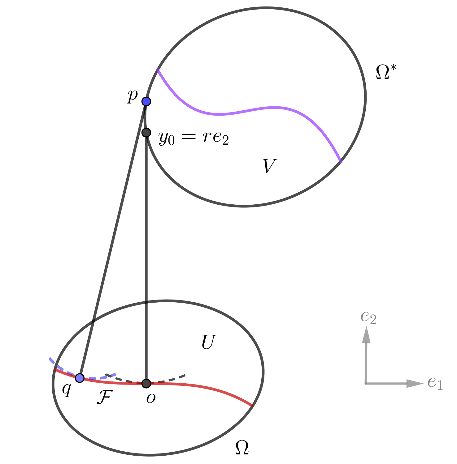
Fig. 5.1.

The next lemma is a refinement of Lemma 5.1.

Lemma 5.2.

$\rho(x_{1})\leq Cx_{1}^{2}$ for $x_{1}$ close to $0$. Moreover, $\rho(x_{1})=\frac{1}{2r}x_{1}^{2}+o(x^{2}_{1})$ for $x_{1}<0$ close to $0$.

Proof.

First, by the interior ball property in Lemma 2.1, $\mathcal{F}$ stays below the ball $B_{r}(y_{0})$, which implies that $\rho(x_{1})\leq\frac{1}{2r}x_{1}^{2}+o(x^{2}_{1})$ for $x_{1}$ close to $0.$ Hence it suffices to prove $\rho(x_{1})\geq\frac{1}{2r}x_{1}^{2}+o(x^{2}_{1})$ for $x_{1}<0$ near the origin.

Consider a point $q=(q_{1},\rho(q_{1}))\in\mathcal{F}$ for $q_{1}<0$ small. Denote $p=Du(q)\in\partial\Omega^{*}$. By the interior ball property again, we have $B_{|p-q|}(p)\cap\Omega\subset U.$ It implies $|p-q|\leq|p-0|,$ since otherwise $0$ would be an interior point of $U$ contradicting to the fact that $0\in\partial U.$ Hence we have

(5.5) $$\begin{split}|p_{2}-\rho(q_{1})|^{2}+(p_{1}+|q_{1}|)^{2}&=|p-q|^{2}\\ &\leq|p|^{2}=p_{1}^{2}+p_{2}^{2}.\end{split}$$

It follows that

$$\rho(q_{1})\geq\frac{1}{2p_{2}}q_{1}^{2}.$$

By the continuity of $Du$, we have $p_{2}\to r$ as $q_{1}\to 0$, namely $p_{2}=r+o(1)$ as $q_{1}\to 0.$ Therefore,

$$\rho(q_{1})\geq\frac{1}{2r+o(1)}q_{1}^{2}\geq\frac{1}{2r}q_{1}^{2}+o(q_{1}^{2}).$$

∎

By our discussion in Section 2, $v\in C^{1}(\mathbb{R}^{2})$ and $Dv=\text{Id}$ in $\Omega\setminus U$. Hence, as $0\in\mathcal{F}\subset\partial U$,

$$Dv(0)=0=Dv(y_{0}).$$

By the convexity of $v$, we infer that

$$Dv(te_{2})=0\quad\forall\,t\in[0,r].$$

By subtracting a constant, we may assume that $v(y_{0})=0$ and $v\geq 0$ on $\mathbb{R}^{2}$. Then $v(te_{2})=0$ for all $t\in[0,r]$ as well.

Consider the point $p=(p_{1},p_{2})\in\partial\{v<h\}\cap\partial\Omega^{*}$ with $p_{2}<r$ (see Fig. 5.2). Since $0\in\{v<h\}$, by the convexity of $\{v<h\}$ and $\Omega^{*}$, the sub-level set

(5.6) $$S_{h}[v]=\{v<h\}\cap\Omega^{*}\ \text{is pinched between the rays}\ \overrightarrow{0y_{0}}\ \text{and}\ \overrightarrow{0p}.$$

Denote $s:=r-p_{2}$. From (5.4), $p_{1}=\rho^{*}(-s)=as^{2}+o(s^{2})$.

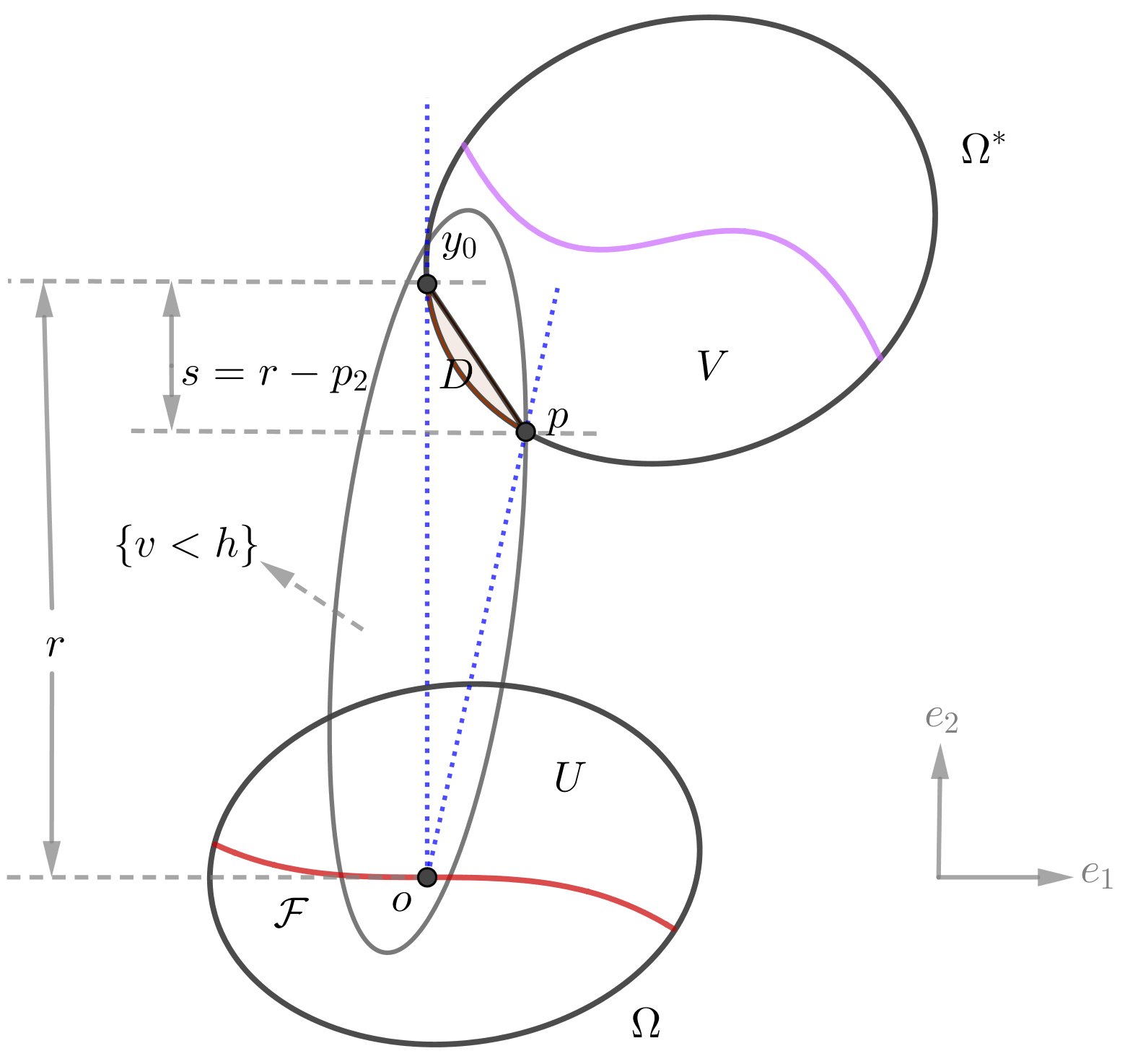
Fig. 5.2.

Lemma 5.3.

There exist positive constants $C_{1},C_{2}$ depending on $\lambda$ and the domains $\Omega,\Omega^{*}$, but independent of $h$, such that

(5.7) $$C_{1}h^{1/3}\leq s\leq C_{2}h^{1/3}.$$

Proof.

Let $D\subset S_{h}[v]$ be the region enclosed by $\partial\Omega^{*}$ and the segment $\overline{y_{0}p}$, (see Fig. 5.2). We have

(5.8) $$\begin{split}|D|&=\frac{1}{2}s\rho^{*}(-s)-\int_{0}^{s}\rho^{*}(-t)\,dt\\ &=\frac{1}{2}as^{3}+o(s^{3})-\int_{0}^{s}(at^{2}+o(t^{2}))\,dt\\ &=\frac{1}{6}as^{3}+o(s^{3}).\end{split}$$

By the volume estimate (2.28), we also have $|D|\leq|S_{h}[v]|\approx h$. Hence, $s\leq C_{2}h^{1/3}$.

For any given $y\in S_{h}[v]$, by (5.6) we have $\frac{y_{1}}{y_{2}}\leq\frac{p_{1}}{p_{2}}.$ By the strict convexity of $v$, we have $\text{diam}(S_{h}[v])\leq\frac{r}{3}$ for $h$ sufficiently small. Hence, $p_{2}\geq\frac{2}{3}r$ and $y_{2}\leq\frac{4}{3}r$, thus we obtain

$$y_{1}\leq\frac{p_{1}}{p_{2}}y_{2}\leq Cs^{2}.$$

From (5.4) we also have

$$y_{1}\geq\rho^{*}(y_{2}-r)\geq\frac{1}{2}a(y_{2}-r)^{2}.$$

Combining the above two inequalities, we obtain $|y_{2}-r|\leq Cs\ \forall\,y\in S_{h}[v]$. Hence

$$S_{h}[v]\text{ is contained in the box }[0,Cs^{2}]\times[r-Cs,r+Cs].$$

It follows that $h\approx|S_{h}[v]|\leq 2C^{2}s^{3}$, which then implies $s\geq C_{1}h^{1/3}$. ∎

Thanks to Lemma 5.3, we are able to give a precise description of the shape of the centred sub-level set $S^{c}_{h}[v](y_{0})$ in the subsequent lemma.

Remark 5.2.

In order to simplify notations, we can translate $y_{0}$ to the origin by letting $\hat{u}(x)=u(x)-y_{0}\cdot x$ and $\hat{v}(y)=v(y+y_{0}).$ By subtracting a constant we may also assume $\hat{u}(0)=\hat{v}(0)=0$, and $D\hat{u}(0)=D\hat{v}(0)=0.$ Under the translation, $V$ becomes $\hat{V}$ defined by (5.2) and

$$D\hat{u}(\mathbb{R}^{2})=\hat{\Omega}^{*}=\left\{y-y_{0}:y\in\Omega^{*}\right\}.$$

By the properties $(i)$–$(iii)$ in §2.1, it is also straightforward to check that $\hat{u}^{*}=\hat{v}$ in $\hat{V}$, and $\hat{u}^{*}$ is strictly convex in $\hat{\Omega}^{*}.$ For simplicity, we denote $\hat{u},\hat{v},\hat{\Omega}^{*},\hat{V}$ by $u,v,\Omega^{*},V$. We remark that the separation of $\Omega^{*}$ and $\Omega$ will not be used in the rest of this subsection.

By Remark 5.2, we may assume $y_{0}=0,v(0)=0$ and $Dv(0)=0.$ The following lemma characterises the shape of the centred sub-level set $S^{c}_{h}[v](0)$.

Lemma 5.4.

There exists a positive constant $C$ independent of $h$ such that

(5.9) $$B_{\frac{1}{C}}(0)\subset A_{h}\big{(}S^{c}_{h}[v]\big{)}\subset B_{C}(0),$$

where $A_{h}$ is a linear transform given by

(5.10) $$A_{h}=\left(\begin{matrix}h^{-\frac{2}{3}},&0\\ 0,&h^{-\frac{1}{3}}\end{matrix}\right).$$

Proof.

Let $D$ be as in the proof of Lemma 5.3. From (5.8) and (5.7), we have the volume estimate $|D|\approx h$. Hence

$$|A_{h}(D)|=\frac{1}{h}|D|\geq\frac{1}{C}$$

for some $C>0$ independent of $h$. Since $D$ is contained in the rectangle $[0,Ch^{2/3}]\times[-Ch^{1/3},0]$, we see that $A_{h}(D)$ is bounded, and $A_{h}(D)\subset B_{C}(0)$ for a constant $C$ independent of $h$. Hence there exist a ball contained in $A_{h}(D)$, namely

$$B_{\frac{1}{C}}(q)\subset A_{h}(D)$$

for a point $q\in A_{h}(D)$ and a different constant $C$. From the equivalence relation (2.30), we thus conclude

(5.11) $$B_{\frac{1}{C}}(q)\subset A_{h}(D)\subset A_{h}(S_{h}[v])\subset A_{h}(S_{bh}^{c}[v]),$$

where $b\geq 1$ is a constant independent of $h$.

By the volume estimate (2.28), we have $|S_{h}[v]|\approx|S_{h}^{c}[v]|\approx h$, hence

(5.12) $$|A_{h}(S_{bh}^{c}[v])|\approx 1.$$

By (5.11), (5.12) and noting that $S_{bh}^{c}[v]$ is a convex set centred at $0$, we obtain (5.9). ∎

The proof of Lemma 5.4 also applies to the sub-level set $S_{h}[v]$. In fact, from (5.11), $A_{h}(S_{h}[v])$ contains a ball $B_{1/C_{1}}(q)$. By John’s lemma, there exists an ellipsoid $E$ centered at $q^{\prime},$ the center of mass of $A_{h}(S_{h}[v]),$ such that $E\subset A_{h}(S_{h}[v])\subset C(n)E.$ Let $r_{1}\leq r_{2}\leq\cdots r_{n}$ be the principal radii of $E.$ Similarly to (5.12), we see that by (2.28), the volume $|A_{h}(S_{h}[v])|\approx 1,$ hence $r_{1}r_{2}\cdots r_{n}\approx 1.$ Since $A_{h}(S_{h}[v])$ contains a ball $B_{1/C_{1}}(q),$ $r_{1}\geq\frac{1}{C_{1}C(n)}.$ Hence $r_{n}\lesssim\frac{1}{r_{1}^{n-1}}\leq C.$ Therefore, $A_{h}(S_{h}[v])$ also has a good shape, namely, $B_{1/C}(q^{\prime})\subset A_{h}(S_{h}[v])\subset B_{C}(q^{\prime}),$ for some positive constant $C$ independent of $h.$

Proof of Proposition 5.1 when $n=2$.

Denote $V_{h}=A_{h}(V)$, $U_{h}=\frac{1}{h}A^{-1}_{h}(U)$. Locally near the origin, the boundary $\partial U_{h}$ can be represented by

(5.13) $$\partial U_{h}=\Big{\{}(x_{1},x_{2})\in\mathbb{R}^{2}:\ x_{2}=\rho_{h}(x_{1}):=h^{-\frac{2}{3}}\rho(h^{\frac{1}{3}}x_{1})\Big{\}}.$$

By Lemma 5.2, we have $\rho_{h}(t)\leq Ct^{2},$ and $\rho_{h}(t)=\frac{1}{2r}t^{2}+o(1)t^{2}$ for $t<0.$

Similarly, by (5.4), the boundary $\partial V_{h}$ can locally be represented by

(5.14) $$\partial V_{h}=\left\{(y_{1},y_{2})\in\mathbb{R}^{2}:\ y_{1}=\rho^{*}_{h}(y_{2})=h^{-\frac{2}{3}}\rho^{*}(h^{\frac{1}{3}}y_{2})=ay_{2}^{2}+o(1)y_{2}^{2}\right\},$$

where $o(1)\rightarrow 0$ as $h\rightarrow 0$.

Denote

(5.15) $$v_{h}(y)=\frac{1}{h}v(A_{h}^{-1}y).$$

We claim that for $h>0$ small, $v_{h}$ is locally uniformly bounded in $\mathbb{R}^{2}$. Note that by (2.15) we have $S^{c}_{h}[v]\cap V=S^{c}_{h}[v]\cap\Omega^{*}$ is convex and $S^{c}_{h}[v]\cap\Omega=\emptyset$ for $h$ small. Hence, by (2.1)

$$C^{-1}\chi_{{}_{S^{c}_{h}[v]\cap V}}\leq\mbox{det}\,D^{2}v\leq C\chi_{{}_{S^{c}_{h}[v]\cap V}}\quad\mbox{ in }S^{c}_{h}[v].$$

Therefore, the Monge-Ampère measure $\mu_{v}$ is doubling for $S^{c}_{h}[v],$ when $h$ is small. Note also that, by the same reason the doubling property holds for all centred sub-level sets $S^{c}_{h}[v](y)$ for $y\in\overline{V}$ close to the origin and $h$ small. Then, for any $k>0$ large, by the geometric decay of sections (see [4, Lemma 2.2] or [5, Lemma 7.6]), there exists a constant $M_{k}$ such that

$$kS^{c}_{h}[v]\subset S^{c}_{M_{k}h}[v]\quad\text{ for $h>0$ small}.$$

On the other hand, by (5.9) we have

$$B_{\frac{k}{C}}(0)\subset A_{h}\left(kS^{c}_{h}[v]\right)\subset A_{h}\left(S^{c}_{M_{k}h}[v]\right).$$

From (2.14), we have $v\leq C_{1}M_{k}h$ in $S^{c}_{M_{k}h}[v]$ for a constant $C_{1}$ independent of $h$. Hence under the normalisation (5.15), we obtain

(5.16) $$0\leq v_{h}\leq C_{1}M_{k}\quad\text{in }B_{\frac{k}{C}}(0),$$

where the constants $C,C_{1}$ are independent of $k,h$. As $k>0$ can be arbitrarily large, the claim is proved. By (5.16), [12, Corollary A.23] and the convexity of $v_{h},$ we have that

(5.17) $$\|Dv_{h}\|_{L^{\infty}(B_{{k}/{2C}}(0))}\leq\frac{\|v_{h}\|_{L^{\infty}(B_{{k}/{C}}(0))}}{{k}/{2C}}\leq\frac{2CC_{1}M_{k}}{k}.$$

Now, passing to a subsequence, by the above claim we may assume that $v_{h}$ converges to $v_{0}$ locally uniformly. By the expression (5.14), we may also assume that $V_{h},\rho^{*}_{h}$ converge to $V_{0},\rho^{*}_{0}$ locally uniformly, and

$$V_{0}:=\big{\{}y\in\mathbb{R}^{2}\,:\,y_{1}>\rho_{0}^{*}(y_{2})=ay_{2}^{2}\big{\}}.$$

Moreover,

(5.18) $$\mbox{det}\,D^{2}v_{0}=c_{0}\chi_{{}_{V_{0}}}\quad\text{ in }\ \mathbb{R}^{2}$$

for some constant $c_{0}>0$.

Denote by $U_{0}$ the interior of $\partial v_{0}(\mathbb{R}^{2})$. Since $v_{0}$ is a convex function defined on entire $\mathbb{R}^{2},$ $U_{0}$ is convex. First we need a property that for any $\tau>0,$ there exists a constant $M_{\tau}>0$ independent of $h$ such that

(5.19) $$B_{\tau}(0)\cap U_{h}\subset Dv_{h}(B_{M_{\tau}}(0)\cap V_{h})\quad\text{ for $h>0$ small}.$$

This property will be proved for general dimension later, see Lemma 5.10 and its proof.

For any $k$ large, by (5.17) we also have

(5.20) $$Dv_{h}(B_{k}(0))\subset B_{{}_{C_{k}}}\cap\overline{U_{h}}\quad\text{ for $h>0$ small}$$

for some constant $C_{k}$ independent of $h.$ By (5.19) and (5.13), we have that

$$\{x:x_{2}>Cx^{2}_{1}\}\cap B_{\tau}(0)\subset Dv_{h}(B_{M_{\tau}}(0)).$$

Let $h\rightarrow\infty,$ and then take $\tau\rightarrow\infty$ (also take $M_{\tau}\rightarrow\infty$) we have that

$$\{x\in\mathbb{R}^{2}:x_{2}>Cx_{1}^{2}\}\subset\partial v_{0}(\mathbb{R}^{2}),$$

which implies

(5.21) $$\{x\in\mathbb{R}^{2}:x_{2}>Cx_{1}^{2}\}\subset U_{0}.$$

By (5.21) and the convexity of $U_{0},$ we have that $U_{0}\subset\{x:x_{2}\geq 0\}.$ Hence $U_{0}$ is the epigraph of some convex function $\rho_{0}$ with $\rho(0)=\rho^{\prime}(0)=0,$ namely, $U_{0}=\{x:x_{2}>\rho_{0}(x)\}.$ Replacing $\{x\in\mathbb{R}^{2}:x_{2}>Cx_{1}^{2}\}$ by $\{x:x_{2}>\rho_{h}(x_{1}),x_{1}<0\}$ in the above argument, we have that $\{x\in\mathbb{R}^{2}:x_{2}>\frac{1}{2r}x_{1}^{2},x_{1}<0\}\subset U_{0},$ which implies $\rho_{0}(x_{1})\leq\frac{1}{2r}x_{1}^{2}$ for $x_{1}<0.$ Note that $\rho_{h}(t)=\frac{1}{2r}t^{2}+o(1)t^{2}$ for $t<0.$

Then, for any $k$ large, since the convex functions $v_{h}$ locally uniformly converges to $v_{0}$ in $\mathbb{R}^{n},$ and both $v_{h},v_{0}$ are $C^{1}$ in the interior of $B_{k}(0)\cap V_{0}$ (provided $h$ is sufficiently small), by convexity we have that $Dv_{h}$ converges to $Dv_{0}$ locally uniformly in $B_{k}\cap V_{0}.$ Hence, $Dv_{h}(x)\rightarrow Dv_{0}(x)$ for any $x\in V_{0}.$ Then, by (5.20) and (5.13), taking limit $h\rightarrow 0,$ we have that $Dv_{0}(V_{0})\cap\{x:x_{1}\leq 0\}\subset\{x:x_{2}\geq\frac{1}{2r}x_{1}^{2}\}.$ By (5.18) we see that $|\partial V_{0}(\mathbb{R}^{2}\backslash V_{0})|=0,$ which implies that $|U_{0}\backslash Dv_{0}(V_{0})|=0.$ Note that the boundary of convex set has Lebesgue measure $0$. From the above discussion we deduce that $U_{0}\cap\{x:x_{1}\leq 0\}\subset\{x:x_{2}\geq\frac{1}{2r}x_{1}^{2}\},$ which implies that $\rho_{0}(x_{1})\geq\frac{1}{2r}x_{1}^{2}$ for $x_{1}<0$.

Therefore, we have

(5.22) $$U_{0}=\Big{\{}(x_{1},x_{2})\in\mathbb{R}^{2}\,:\,x_{2}>\rho_{0}(x_{1})\Big{\}}$$

where $\rho_{0}$ is a convex function satisfying $0\leq\rho_{0}(t)\leq Ct^{2}$ and $\rho_{0}(t)=\frac{1}{2r}t^{2}$ for $t<0.$ Hence $U_{0}\subset\{x_{2}\geq 0\}$ and $\{x_{2}=0\}$ is a support plane of $U_{0}$ at $0$.∎

5.2. Blow-up in higher dimensions

In this subsection we assume $n\geq 3$ and the obliqueness fails at $x_{0}\in\mathcal{F}.$ Similarly as in §5.1, denote $y_{0}=Du(x_{0})$, which is a point on $\partial V\setminus\overline{\partial V\cap\Omega^{*}}\subset\partial\Omega^{*}$. Denote still by $\nu_{{}_{U}}(x_{0}),\nu_{{}_{V}}(y_{0})$ the unit inner normals of $U,V$ at $x_{0},y_{0}$, respectively. By a change of coordinates, we assume that $x_{0}=0$, $\nu_{{}_{U}}(0)=e_{n}$, and $\nu_{{}_{V}}(y_{0})=e_{1}$. By subtracting a constant we can also assume that $v\geq 0$ and $v(y_{0})=0$. From (2.11), $y_{0}=re_{n}$ for some $r>0$.

Unless otherwise specified, we use the notations $x=(x_{1},\cdots,x_{n})\in\mathbb{R}^{n}$; $x^{\prime}=(x_{1},\cdots,x_{n-1})$, $\hat{x}=(x_{2},\cdots,x_{n})\in\mathbb{R}^{n-1}$; and $\tilde{x}=(x_{2},\cdots,x_{n-1})\in\mathbb{R}^{n-2}$.

Similarly to (5.3), the free boundary $\mathcal{F}$ can locally be expressed by

$$\mathcal{F}=\{x\,:\,x_{n}=\rho(x_{1},\tilde{x})\}\ \ \ \text{near $0$}$$

for some function $\rho$. By Lemma 2.1, $\mathcal{F}$ lies below the ball $B_{r}(y_{0})$ near $0$. Hence by $ii)$ of Theorem 2.1, the function $\rho$ satisfies

(5.23) $$-C(x_{1}^{2}+|\tilde{x}|^{2})^{\frac{1+\alpha^{\prime}}{2}}\leq\rho(x_{1},\tilde{x})\leq C(x_{1}^{2}+|\tilde{x}|^{2})$$

for some $\alpha^{\prime}\in(0,1)$. Analogously to (5.4), we also have

$$\partial V=\left\{y\,:\,y_{1}=\rho^{*}(\tilde{y},y_{n}-r)\right\}\quad\text{ near }\ y_{0}$$

for some $C^{2}$ smooth and uniformly convex function $\rho^{*}$, which can be expressed as

(5.24) $$\rho^{*}(\tilde{y},t)=P(\tilde{y},t)+o(|\tilde{y}|^{2}+t^{2}),$$

where $P$ is a quadratic polynomial satisfying

$$C^{-1}(|\tilde{y}|^{2}+t^{2})\leq P(\tilde{y},t)\leq C(|\tilde{y}|^{2}+t^{2})$$

for some positive constant $C$.

For brevity, we write $S_{h}[v](y_{0}),S_{h}^{c}[v](y_{0})$ simply as $S_{h}[v],S^{c}_{h}[v]$ when no confusion arises. By $(ii)$ of Corollary 2.1, for any given $\varepsilon>0$, there exists $C_{\varepsilon}$ such that

(5.25) $$\begin{split}&B_{C_{\epsilon}h^{\frac{1}{2}+\epsilon}}(y_{0})\cap\{y_{1}=0\}\subset S_{h}^{c}[v].\\ \end{split}$$

A key estimate is the following

Lemma 5.5.

For any given $\epsilon>0$ small, there exists a constant $C_{\epsilon}$ such that for all unit vector $e\in\text{span}\{e_{2},e_{3},\cdots,e_{n-1}\}$,

(5.26) $$|(y-y_{0})\cdot e|\leq C_{\epsilon}h^{\frac{1}{2}-\epsilon}\quad\forall\,y\in S_{h}^{c}[v].$$

Let $p=(p_{1},0,\cdots,0,p_{n})$ be a point on $\partial\{v<h\}\cap\partial\Omega^{*}$ with $p_{n}<r$ (see Fig. 5.3). Denote $s=r-p_{n}$. Since $\partial\Omega^{*}$ is $C^{2}$ smooth and uniformly convex, we have $p_{1}=as^{2}+o(s^{2})$ for a positive constant $a.$ Lemma 5.5 is built upon the following estimate.

Lemma 5.6.

For any $\epsilon>0$ small, there exist constants $C,C_{\epsilon}$ such that

(5.27) $$Ch^{\frac{1}{3}}\leq s\leq C_{\epsilon}h^{\frac{1}{3}-\epsilon}$$

when $h>0$ is small, where $C>0$ is a constant independent of $\varepsilon$.

Proof.

Let $D\subset\text{span}\{e_{1},e_{n}\}$ be a two-dimensional region enclosed by $\partial\Omega^{*}$ and the segment $\overline{y_{0}p}$ (see Fig. 5.3). By (5.8), we have $|D|_{\mathcal{H}_{2}}=\frac{1}{6}as^{3}+o(s^{3})$, where $|\cdot|_{\mathcal{H}_{d}}$ denotes the $d$-dimensional Hausdorff measure. From (2.30), we have

(5.28) $$D\subset S_{h}[v]\cap V\subset S_{bh}^{c}[v].$$

By (5.25) we have

(5.29) $$C_{\epsilon}h^{\frac{1}{2}+\epsilon}e_{i}\subset S^{c}_{bh}\quad\text{for}\ i=2,\cdots,n-1.$$

Combining these estimates and using (2.28) and the convexity of $S^{c}_{bh}$, we obtain

$$h^{\frac{n}{2}}\approx|S_{bh}^{c}|_{\mathcal{H}_{n}}\geq C_{\epsilon}h^{(\frac{1}{2}+\epsilon)(n-2)}|D|_{\mathcal{H}_{2}}\geq C_{\epsilon}s^{3}h^{(\frac{1}{2}+\epsilon)(n-2)}.$$

Hence the second inequality of (5.27) is obtained.

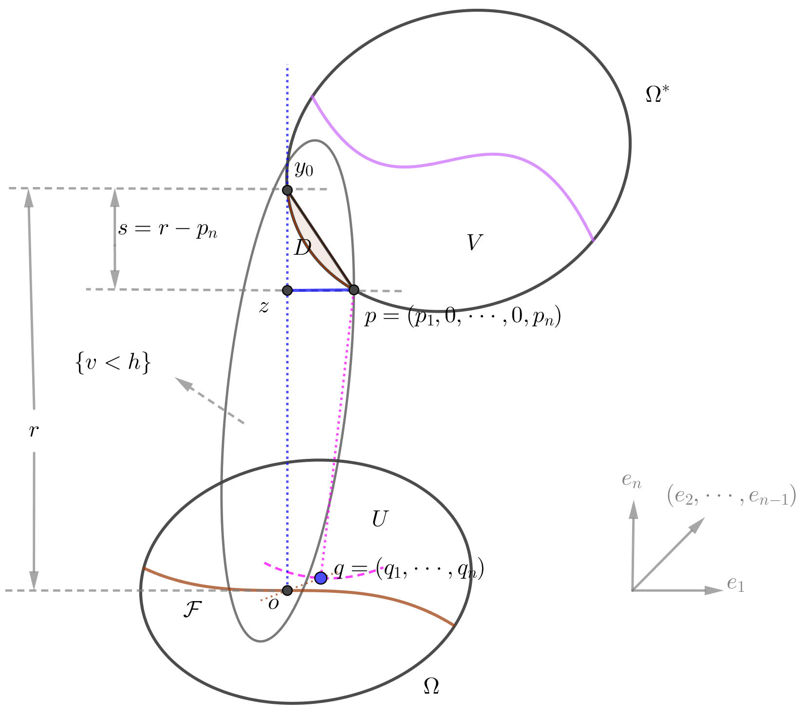
Fig. 5.3.

Next we show the first inequality of (5.27). By the reasoning before Lemma 5.3, we may assume that $v\geq 0$ in $\mathbb{R}^{n}$, $v(0)=v(y_{0})=0$, and $v=0$ on the segment $\overline{0y_{0}}$. In particular, we have $v(z)=0$, where $z=p_{n}e_{n}$ is the projection of $p$ on the $x_{n}$ axis. Denote $q=(q_{1},\cdots,q_{n})=Dv(p)\in\mathcal{F}$. By the convexity of $v$, we have

(5.30) $$q_{1}=Dv(p)\cdot e_{1}\geq\frac{v(p)-v(z)}{|p-z|}=\frac{h}{p_{1}}\geq C\frac{h}{s^{2}}.$$

By the interior ball property (Lemma 2.1), we have $B_{|p-q|}(p)\cap\Omega\subset U$. Hence

(5.31) $$|p-q|^{2}\leq|p-0|^{2}.$$

By the interior ball property again, the free boundary $\mathcal{F}$ lies below the ball $B_{r}(y_{0})$. It implies

(5.32) $$q_{n}\leq r-\sqrt{r^{2}-|q^{\prime}|^{2}},$$

where $q^{\prime}=(q_{1},q_{2},\cdots,q_{n-1})$.

Note that when $h>0$ is sufficiently small, by strict convexity of $v$ in $V$, $S_{h}[v]$ will be small, and then by the continuity of $Dv$, $|q|$ will be small, which ensures $|q^{\prime}|<r$ and $p_{n}>r-\sqrt{r^{2}-|q^{\prime}|^{2}}.$ Recall that $p_{n}=r-s$. By (5.31) and (5.32), we have

$$|q^{\prime}|^{2}+p_{1}^{2}-2p_{1}q_{1}+\big{(}r-s-(r-\sqrt{r^{2}-|q^{\prime}|^{2}})\big{)}^{2}\leq p_{1}^{2}+(r-s)^{2},$$

from which one infers that

$$2sr \leq 2p_{1}q_{1}+2sr\Big{(}1-\frac{|q^{\prime}|^{2}}{r^{2}}\Big{)}^{\frac{1}{2}}$$

$$\leq 2p_{1}q_{1}+2sr-\frac{s}{r}|q^{\prime}|^{2}.$$

Namely $\frac{s}{r}|q^{\prime}|^{2}\leq 2p_{1}q_{1}$. Noting that $q_{1}\leq|q^{\prime}|$, we thus obtain

$$\frac{s}{r}q_{1}\leq 2p_{1}.$$

Recall that $p_{1}\leq Cs^{2}+o(s^{2})$. By (5.30), we then deduce

$$\frac{h}{sr}\leq Cp_{1}\leq Cs^{2},$$

from which it follows that $s\geq Ch^{\frac{1}{3}}$. So the first inequality of (5.27) is proved. ∎

With Lemma 5.6, we are now ready to prove Lemma 5.5.

Proof of Lemma 5.5.

Let $D$ be the region defined in the proof of Lemma 5.6, (see Fig. 5.3). By (5.28),

(5.33) $$D\subset S_{bh}^{c}[v].$$

From (5.8) and thanks to (5.27), we have

(5.34) $$|D|_{\mathcal{H}_{2}}=\frac{1}{6}as^{3}+o(s^{3})\geq Ch,$$

provided $h>0$ is small enough.

Let $e\in\text{span}\{e_{2},e_{3},\cdots,e_{n-1}\}$ be a unit vector. Denote by $e^{\perp}$ the subspace orthogonal to $e$, passing through the point $y_{0}$. Then by (5.25), (5.33) and (5.34), we have

$$|S_{bh}^{c}[v]\cap e^{\perp}|_{\mathcal{H}_{(n-1)}}\geq Ch^{(\frac{1}{2}+\epsilon)(n-3)}|D|_{\mathcal{H}_{2}}\geq C_{\epsilon}h^{1+(\frac{1}{2}+\epsilon)(n-3)}.$$

Hence, $\forall\,y\in S_{bh}^{c}[v]$, by the convexity of $S_{bh}^{c}[v]$ and the volume estimate (2.28) we obtain

$$\begin{split}h^{n/2}\approx|S_{bh}^{c}[v]|_{\mathcal{H}_{n}}&\geq|S_{bh}^{c}[v]\cap e^{\perp}|_{\mathcal{H}_{(n-1)}}\times|(y-y_{0})\cdot e|\\ &\geq C_{\epsilon}h^{1+(\frac{1}{2}+\epsilon)(n-3)}|(y-y_{0})\cdot e|,\end{split}$$

which implies that $|(y-y_{0})\cdot e|\leq C_{\epsilon}h^{\frac{1}{2}-(n-3)\epsilon}$. Note that the constant $b$ in (2.30) is independent of $h$. Replacing $h$ with ${h}/{b}$, we then obtain the desired estimate (5.26). ∎

Corollary 5.1.

For any $y\in S_{h}[v]$, we have

$$Dv(y)\cdot e_{n}\geq-C_{\epsilon}h^{1-\epsilon}\ \ \ \text{for $h>0$ small. }$$

Proof.

For any given $y\in S^{c}_{h}[v]\cap V$, by Lemma 5.5,

(5.35) $$|y_{i}|\leq C_{\epsilon}h^{\frac{1}{2}-\epsilon}\ \ \ \text{for}\ i=2,\cdots,n-1.$$

From (5.25), $B_{C_{\epsilon}h^{\frac{1}{2}+\epsilon}}(y_{0})\cap\{y_{1}=0\}\subset S^{c}_{h}[v].$ Hence by (2.28), we have

$$h^{\frac{n}{2}}\approx|S_{h}^{c}[v]|\geq C_{\epsilon}^{n-1}h^{(\frac{1}{2}+\epsilon)(n-1)}y_{1},$$

which implies

(5.36) $$y_{1}\leq C_{\epsilon}h^{\frac{1}{2}-(n-1)\epsilon}.$$

For any given $y\in S_{h}[v]$, by the equivalence relation (2.30), the above estimates (5.35) and (5.36) also hold. By Lemma 2.1, similarly to (5.31) we have $|y-Dv(y)|\leq|y|$. Hence if $Dv(y)\cdot e_{n}<0$, we have

$$|Dv(y)\cdot e_{n}| \leq|y|-y_{n}=\sqrt{y_{1}^{2}+\cdots+y_{n-1}^{2}+y_{n}^{2}}-y_{n}$$

(5.37) $$\leq\frac{C}{y_{n}}(y_{1}^{2}+\cdots+y_{n-1}^{2}).$$

When $h>0$ is small, $y$ is close to $y_{0}$ and $y_{n}\geq\frac{r}{2}$. Combining (5.35), (5.36) and (5.2), we obtain $Dv(y)\cdot e_{n}\geq-C_{\epsilon}h^{1-\epsilon}.$ ∎

In the rest of the section, we will not use the condition that $\Omega^{*}$ and $\Omega$ are separate anymore. By the changes in Remark 5.2, we may assume $y_{0}=0$ for simplicity. Let $T_{h}$ be an affine transformation such that $T_{h}(S_{h}^{c}[v])\sim B_{1}(0)$. Let $T_{1}:y\mapsto\bar{y}$ be the transform given by

(5.38) $$\left\{{\begin{array}[]{ll}\bar{y}_{1}=h^{-\frac{2}{3}}y_{1},&\\ \bar{y}_{i}=h^{-\frac{1}{2}}y_{i},&\ \ \ i=2,\cdots,n-1,\\ \bar{y}_{n}=h^{-\frac{1}{3}}y_{n}.&\end{array}}\right.$$

The following lemma shows that $T_{h}$ is close to $T_{1}$, in the sense that the norm of $T_{2}:=T_{h}\circ T_{1}^{-1}$ is bounded by $h^{-\epsilon}$ for any $\epsilon>0$, when $h>0$ small. It provides geometric estimates for the shape of the centred sub-level set $S^{c}_{h}[v]$.

Lemma 5.7.

For any $\epsilon>0$, there exists a constant $C_{\epsilon}>0$ independent of $h$ such that

(5.39) $$B_{\frac{1}{C_{\epsilon}}h^{\epsilon}}\subset T_{1}(S_{h}^{c}[v])\subset B_{C_{\epsilon}h^{-\epsilon}},$$

and

(5.40) $$\|T_{2}\|+\|T_{2}^{-1}\|\leq C_{\epsilon}h^{-\epsilon}.$$

Proof.

Let $b$ be the constant in (2.30). By (5.25) we have that

(5.41) $$B_{C_{\epsilon}h^{\frac{1}{2}+\epsilon}}(0)\cap\{y_{1}=0\}\subset S^{c}_{bh}[v].$$

Let $D$ be domain in the $x_{1}x_{n}$-plane, given in the proof of Lemma 5.6. Let $G$ be the convex hull of the set $D\cup\{C_{\epsilon}h^{\frac{1}{2}+\epsilon}e_{i}:i=2,\cdots,n-1\}.$ Since $D\subset S_{h}[v]\subset S_{bh}^{c}[v]$, by (5.25) we have $G\subset S_{bh}^{c}[v].$

By Lemma 5.6, we have

$$T_{1}(G)\subset B_{C_{\epsilon}h^{-c_{{}_{1}}\epsilon}}(0)\ \ \text{ and }\ \ |T_{1}(G)|\geq C_{\epsilon}h^{c_{{}_{2}}\epsilon}$$

for some constants $c_{{}_{1}},c_{{}_{2}}>0$. Note that the first inclusion uses $p_{1}=as^{2}+o(s^{2})\lesssim h^{\frac{2}{3}-2\epsilon},$ and the second inequality use (5.8), the estimate on $|D|_{\mathcal{H}_{2}}.$

By convexity, it implies that there exists a ball

(5.42) $$B_{C_{\epsilon}h^{c_{{}_{3}}\epsilon}}(z)\subset T_{1}(G)$$

for some point $z\in T_{1}(G)$ and some constant $c_{{}_{3}}>0$. As $\epsilon>0$ can be arbitrarily small, we may simply assume that $c_{{}_{3}}=1$.

Since $T_{1}(G)\subset T_{1}(S_{bh}^{c}[v])$ and $|T_{1}(S_{bh}^{c}[v])|\approx 1$, by (5.42) we have

$$\text{diam}(T_{1}(S_{bh}^{c}[v]))\leq C_{\epsilon}h^{-(n-1)\epsilon}.$$

By John’s Lemma [4, Lemma 2.1], there exists an ellipsoid $E$ centred at $0,$ such that $E\subset T_{1}(S_{bh}^{c}[v])\subset CE$ for some constant $C$ depending only on $n.$ Let $r_{1}\leq\cdots\leq r_{n}$ be the principal semi-axes of $E$. Then we have $r_{n}\leq C_{\epsilon}h^{-(n-1)\epsilon}$ and $r_{1}r_{2}\cdots r_{n}\approx|T_{1}(S_{bh}^{c}[v])|\approx 1$, which implies $r_{1}\geq\frac{1}{C_{\epsilon}}h^{(n-1)^{2}\epsilon}.$ Therefore we obtain (5.39).

Recall that $T_{2}\circ T_{1}(S_{h}^{c}[v])=T_{h}(S_{h}^{c}[v])\sim B_{1}$. By (5.39) we have (5.40). ∎

Remark 5.3.

Note that since $T_{h}(S^{c}_{h}[v])\sim B_{1}(0),$ by (2.30) the equivalence relation between $S^{c}_{h}[v]$ and $S_{h}[v]$ we have that $T_{h}(S_{h}[v])$ also has a good shape and satisfies

(5.43) $$B_{\frac{1}{C}}(0)\cap T_{h}(V)\subset T_{h}(S_{h}[v])\subset B_{C}(0)\cap T_{h}(V)$$

for some constant $C>0$ independent of $h.$

With Lemma 5.7 for the geometric estimate of the sub-level set $S^{c}_{h}[v]$, we can now carry out the normalisation process. Let

(5.44) $$v_{h}(y):=\frac{1}{h}v(T_{h}^{-1}y).$$

Similarly to the claim following (5.15), $v_{h}$ is locally uniformly bounded in $\mathbb{R}^{n}$ as $h\to 0$. Hence by passing to a subsequence, $v_{h}\rightarrow v_{0}$, $T_{h}(V)\rightarrow V_{0}$ locally uniformly, and $v_{0}$ satisfies

(5.45) $$\mbox{det}\,D^{2}v_{0}=c_{0}\chi_{{}_{V_{0}}}\quad\text{in }\mathbb{R}^{n}$$

for a constant $c_{0}>0$. Here by $T_{h}(V)\rightarrow V_{0}$ locally uniformly we mean that for any fixed $k>0$ large, $T_{h}(V)\cap B_{k}(0)$ converges to $V_{0}\cap B_{k}(0)$ as $h\rightarrow 0$ in Hausdorff distance. Note that $T_{h}(V)\cap B_{k}(0)$ is convex when $h$ is sufficiently small. Since for any fixed $k>0,$ we have the diameter of $T_{h}(V)\cap B_{k}(0)$ is uniformly bounded for all $h$ small, hence by the Blaschke selection theorem that up to a subsequence we have $T_{h}(V)\cap B_{k}(0)$ converges to a convex set. Then by the standard diagonal method, we can choose a subsequence such that $T_{h}(V)\rightarrow V_{0}$ locally uniformly.

Since $V_{0}$ is convex, the doubling property holds for the centred sub-level sets of $v_{0}$, namely

$$\Big{|}\frac{1}{2}S_{h}^{c}[v_{0}](y)\cap V_{0}\Big{|}\geq C\Big{|}S_{h}^{c}[v_{0}](y)\cap V_{0}\Big{|}\quad\forall\ y\in\overline{V_{0}},$$

where the constant $C$ depends only on $n$. As $v_{0}$ is a global convex function, $\partial v_{0}(\mathbb{R}^{n})$ is also convex. Hence, by (5.45) and Caffarelli’s boundary regularity theory [3], $v_{0}$ is strictly convex and $C^{1}$ smooth in $\overline{V_{0}}$. However, unlike (5.22) in dimension two, we do not have any further information on the regularity of $\partial U_{0}$, where $U_{0}$ is the interior of $\partial v_{0}(\mathbb{R}^{n})$. Thus we cannot infer higher regularity of $v_{0}$ at the moment. To overcome this difficulty, our strategy is to show that the blow-up limits $U_{0},V_{0}$ have nice decomposition properties (Lemmas 5.9–5.14).

Denote $V_{h}=T_{h}(V)$. The following lemma shows that in the normalisation (5.44), the modulus of convexity and the $C^{1,\alpha^{\prime}}$ norm of $v_{h}$ are locally uniformly bounded as $h\to 0$.

Lemma 5.8.

There exist constants $\alpha^{\prime}\in(0,1]$ and $\beta^{\prime}\geq 2$ such that

(5.46) $$C_{1}|y|^{\beta^{\prime}}\leq v_{h}(y)\leq C_{2}|y|^{1+\alpha^{\prime}}\quad\text{ for }y\in B_{1}(0)\cap V_{h},$$

where the positive constants $C_{1}$ and $C_{2}$ are independent of $h.$

Proof.

Since $T_{h}(S_{h}^{c}[v])\sim B_{1}$, by Remark 5.3 $T_{h}(S_{h}[v])$ has a good shape and

(5.47) $$B_{\frac{1}{C}}(0)\cap V_{h}\subset T_{h}(S_{h}[v])\subset B_{C}(0)\cap V_{h}$$

for a constant $C$ independent of $h.$

The geometric decay estimate (see [4, Lemma 2.2] or [5, Lemma 7.6]) implies that for any given $s_{1}<1,$ there exists a constant $s_{0}<1$ independent of $h$ such that

(5.48) $$S^{c}_{\bar{s}h}[v]\subset s_{1}S^{c}_{h}[v]\quad\ \forall\,\bar{s}\in(0,s_{0}).$$

Since (5.48) is invariant under the normalisation (5.44), the inclusion (5.48) still holds for $v_{h},$ namely, given $h$ small we have

(5.49) $$S^{c}_{\bar{s}\tilde{h}}[v_{h}]\subset s_{1}S^{c}_{\tilde{h}}[v_{h}]\quad\ \forall\,\bar{s}\in(0,s_{0}).$$

for $\tilde{h}<1.$ Choose $s_{1}=\frac{1}{2}$ and let $\bar{s}=\frac{1}{4}s_{0}<\frac{1}{4}.$ By (5.47) we have $B_{\frac{1}{C}}(0)\subset S^{c}_{1}(v_{h})\subset B_{C}(0).$ For any $y\in B_{1}(0)\cap V_{h},$ let $k$ be the positive integer satisfying

(5.50) $$C2^{-k}<|y|\leq C2^{-k+1}.$$

By (5.49), we have $y\notin\frac{1}{2^{k}}S_{1}^{c}[v_{h}]\supset S^{c}_{\bar{s}^{k}}[v_{h}].$ By (2.30), we have $S^{c}_{\bar{s}^{k}}[v_{h}]\cap V_{h}\supset S_{b^{-1}\bar{s}^{k}}[v_{h}].$ Hence $v_{h}(y)\geq b^{-1}\bar{s}^{k}.$ From (5.50), it follows that $k\geq\frac{\log(2C)-\log|y|}{\log 2}.$ Therefore, $v_{h}(y)\geq C_{1}|y|^{\beta^{\prime}},$ where $C_{1}=b^{-1}\bar{s}^{\frac{\log(2C)}{\log 2}},$ and $\beta^{\prime}=-\frac{\log\bar{s}}{\log 2}.$

To prove the second inequality, we claim that there exists a constant $\delta>0$ such that

(5.51) $$v(\frac{1}{2}z)\leq\frac{1}{2}(1-\delta)v(z)\ \ \text{for any $z\in B_{1}(0)\cap V.$}$$

Indeed, if the claim fails, then there exist $\delta_{k}\rightarrow 0$, $z_{k}\in B_{1}(0)\cap V$ such that

$$v(\frac{1}{2}z_{k})\geq\frac{1}{2}(1-\delta_{k})v(z_{k}).$$

The strict convexity of $v$ implies that $z_{k}\rightarrow 0$ and $h_{k}:=v(z_{k})\rightarrow 0$ as $k\rightarrow\infty.$ Denote $\hat{z}_{k}=T_{h_{k}}z_{k}.$ Then we have $v_{h_{k}}(\hat{z}_{k})=1$ and

$$v_{h_{k}}(\frac{1}{2}\hat{z}_{k})\geq\frac{1}{2}(1-\delta_{k})v_{h_{k}}(\hat{z}_{k}).$$

By passing to a subsequence, we may assume that $\hat{z}_{k}\rightarrow z_{0}\in\overline{V_{0}}$ and $v_{0}(\frac{1}{2}z_{0})=\frac{1}{2}v_{0}(z_{0}).$ By convexity, we see that $v_{0}$ is linear on the segment $\overline{0z_{0}},$ which contradicts to the strict convexity of $v_{0}$ in $\overline{V_{0}}.$ Hence, the claim (5.51) is proved.

Since (5.51) is invariant under the normalisation (5.44), it also holds for $v_{h}$. Hence $v_{h}(\frac{1}{2}y)\leq\frac{1}{2}(1-\delta)v_{h}(y)$ for $y\in B_{\frac{1}{C}}(0)\cap V_{h}.$ By iteration we obtain $v_{h}(\frac{1}{2^{k}}y)\leq\frac{1}{2^{k}}(1-\delta)^{k}v_{h}(y)$. Hence there exist constants $\alpha^{\prime}\in(0,1]$ and $C_{2}>0$, independent of $h$, such that $v_{h}(y)\leq C_{2}|y|^{1+\alpha^{\prime}}$ for $y\in B_{1}(0)\cap V_{h}.$ ∎

Lemma 5.9.

For the limit $V_{0}=\lim_{h\to 0}V_{h}$, we have the decomposition

(5.52) $$V_{0}=\omega_{0}^{*}\times H^{*}_{0},$$

where $H^{*}_{0}$ is an $n-2$ dimensional subspace of $\mathbb{R}^{n}$, $\omega_{0}^{*}\subset(H^{*}_{0})^{\perp}:=\{y\in\mathbb{R}^{n}:y\perp H^{*}_{0}\}$ is convex, and $\omega_{0}^{*}$ is smooth. Moreover, $\omega_{0}^{*}$ can be represented as an epigraph of some convex function.

Proof.

Recall that the boundary $\partial V$ is uniformly convex and is given by the function $\rho^{*}$ in (5.24). Let $e\in H:=\text{span}\{e_{2},e_{3},\cdots,e_{n-1}\}$ be any given unit vector. Let

$$z=te+\rho^{*}(te)e_{1}\in\partial V$$

be a boundary point, where $t=h^{\frac{1}{2}-2\epsilon}$ and $\epsilon>0$ is sufficiently small. Let’s track the behaviour of the point $z$ under the affine transformation $T_{h}=T_{2}\circ T_{1}$.

By (5.38), we see that $T_{1}z=h^{-2\epsilon}e+h^{-2/3}\rho^{*}(te)e_{1}$. Hence by (5.40) we have

(5.53) $$|T_{h}z|\geq C_{\epsilon}h^{-\epsilon}\rightarrow\infty\quad\text{ as }h\rightarrow 0.$$

Meanwhile, since $0\leq\rho^{*}(te)\leq Ct^{2}=Ch^{1-4\epsilon}$, by (5.40) we also have

(5.54) $$\text{dist}(T_{h}z,T_{h}H)\leq\|T_{2}\|h^{-2/3}\rho^{*}(te)\leq C_{\epsilon}h^{\frac{1}{3}-5\epsilon}\rightarrow 0\quad\text{ as }h\rightarrow 0.$$

Up to a subsequence, we assume that $T_{h}H$ converges to an $n-2$ dimensional subspace $H_{0}^{*}$ in the sense that $T_{h}H\cap B_{k}(0)$ converges to $H_{0}^{*}\cap B_{k}(0)$ in Hausdorff distance, for all given $k>0.$ Indeed, since $T_{h}H$ is an $n-2$ dimensional subspace, we may assume $T_{h}H$ to be the orthogonal complement of $\text{span}\{e_{1h},e_{nh}\}$ with two orthogonal unit vectors $e_{1h}$ and $e_{nh}.$ Then since $e_{1h},e_{nh}\in\mathbb{S}^{n}$, up to a subsequence we may assume $e_{1h},e_{nh}$ converges to $e_{10},e_{n0}$, respectively. Let $H_{0}^{*}$ be the $n-2$ dimensional subspace orthogonal to $\text{span}\{e_{10},e_{n0}\},$ then we have the desired convergence as above.

Given any $y\in H_{0}^{*},$ by the discussion above, we have that there exists a point $y_{h}\in T_{h}H$ such that $y_{h}\rightarrow y$ as $h\rightarrow 0.$ Let $e_{h}:=\frac{T_{h}^{-1}y_{h}}{|T_{h}^{-1}y_{h}|},$ and $z_{h}=te_{h}+\rho^{*}(te_{h})e_{1}\in\partial V,$ where $t=|T_{h}^{-1}y_{h}|$ provided $h$ is small enough. Then, by (5.40) we have that $t\leq\frac{1}{C_{\epsilon}}h^{\frac{1}{2}-\epsilon}.$ By the same computation leading to (5.54), we have that $\text{dist}(T_{h}z_{h},T_{h}(te_{h}))\rightarrow 0$ as $h\rightarrow 0.$ Note that $T_{h}(te_{h})=y_{h}\rightarrow y$ as $h\rightarrow 0.$ Hence $\partial V_{h}\ni T_{h}z_{h}\rightarrow y$ as $h\rightarrow 0,$ which implies that $y\in\partial V_{0}.$ Hence, $H_{0}^{*}\subset\partial V_{0}.$ By the convexity of $V_{0}$, it follows that $V_{0}=\omega_{0}^{*}\times H^{*}_{0}$, where $\omega_{0}^{*}$ is a convex set in $(H^{*}_{0})^{\perp}.$

Next we prove the smoothness of $\omega_{0}^{*}.$ From (5.24), one sees that

(5.55) $$\tilde{e}_{h}:=\frac{(T_{h}^{t})^{-1}e_{1}}{|(T_{h}^{t})^{-1}e_{1}|}$$

is the unit inner normal of $V_{h}$ at $0$, where $T_{h}^{t}$ is the transpose of $T_{h}$ as a matrix. Denote the unit vector $\tilde{e}^{\prime}_{h}=\frac{T_{h}^{-1}(T_{h}^{t})^{-1}e_{1}}{|T_{h}^{-1}(T_{h}^{t})^{-1}e_{1}|},$ namely $T_{h}\tilde{e}^{\prime}_{h}$ is in the direction of $\tilde{e}_{h}.$ By the definition of $T_{h},$ a direct computation shows that

(5.56) $$\tilde{e}^{\prime}_{h}\cdot e_{1}\geq C_{\epsilon}h^{4\epsilon}.$$

By the $C^{2}$ regularity of $\partial V$ at 0 (see (5.24)) we have $x_{h}=(x_{1},x_{2},\cdots,x_{n}):=h^{6\epsilon}\tilde{e}^{\prime}_{h}\in V$ provided $h$ is small. Indeed, by (5.56) we have

$$x_{1}=h^{6\epsilon}\tilde{e}^{\prime}_{h}\cdot e_{1}\geq C_{\epsilon}h^{10\epsilon}\gg h^{12\epsilon}\geq\sum_{i=2}^{n}|x_{i}|^{2}$$

for $h$ small, which implies that $x_{h}\in V.$ Hence

(5.57) $$T_{h}x_{h}=|T_{h}x_{h}|\tilde{e}_{h}\in V_{h}.$$

By the definition of $T_{h}$ we have

(5.58) $$|T_{h}x_{h}|\geq C_{\epsilon}h^{-\frac{1}{3}+7\epsilon}\rightarrow\infty\ \ \text{ as }\ h\rightarrow 0.$$

Extend the quadratic polynomial $P$ in (5.24) to $\mathbb{R}^{n}$ such that

$$\tilde{P}(y_{1},\hat{y})=P(\hat{y}),\quad\hat{y}=(y_{2},\cdots,y_{n}).$$

Recall that, by (5.24),

$$\partial V=\left\{(y_{1},\hat{y})\,:\,y_{1}=P(\hat{y})+o(P)\right\}\ \ \text{ near }0.$$

By a straightforward computation, we have

(5.59) $$\partial V_{h}=\big{\{}y\,:\,\langle y,\tilde{e}_{h}\rangle=\tilde{P}_{h}(y)+o(\tilde{P}_{h})\big{\}}\ \ \text{ near }0,$$

where $\tilde{P}_{h}(y)=\frac{1}{|(T_{h}^{t})^{-1}e_{1}|}\tilde{P}(T_{h}^{-1}y)\geq 0$, and

(5.60) $$B_{1}(0)\cap V_{h}\subset\Big{\{}y\,:\,\langle y,\tilde{e}_{h}\rangle\geq\frac{1}{2}\tilde{P}_{h}(y)\Big{\}}\ \ \text{ for $h>0$ small}.$$

We claim that the coefficients of the quadratic polynomial $\tilde{P}_{h}$ are uniformly bounded as $h\to 0$. Assume the claim for a moment. Then by passing to a subsequence, we have $\tilde{e}_{h}\rightarrow e_{0}^{*},\tilde{P}_{h}\rightarrow\tilde{P}_{0}$ for a unit vector $e_{0}^{*}$ and a quadratic polynomial $\tilde{P}_{0}$. Moreover, the higher order term $o(\tilde{P}_{h})$ in (5.59) converges to $0$ locally uniformly as $h\to 0$. Hence $\partial V_{0}=\{y\,:\,\langle y,e_{0}^{*}\rangle=\tilde{P}_{0}\}$ is smooth, which implies that $\omega_{0}^{*}$ is smooth. By (5.57), (5.58) and convexity of $V_{0},$ passing to limit, we have

(5.61) $$\{te_{0}^{*}:t>0\}\subset V_{0},$$

which implies that $w^{*}_{0}$ is an epigraph of some convex function.

It remains to prove the above claim. Let $d_{h}$ be the largest coefficient of $\tilde{P}_{h}$. Suppose by contrary that $d_{h}\rightarrow\infty$ as $h\rightarrow 0$. Then $\frac{1}{d_{h}}\tilde{P}_{h}$ has bounded coefficients, and up to a subsequence we assume that $\frac{1}{d_{h}}\tilde{P}_{h}\rightarrow\tilde{P}_{*}$ for a quadratic polynomial $\tilde{P}_{*}$ whose largest coefficient equals $1$. Hence by (5.60),

$$B_{1}(0)\cap V_{h}\subset B_{1}(0)\cap\Big{\{}y\,:\,\frac{1}{d_{h}}\langle y,\tilde{e}_{h}\rangle\geq\frac{1}{2d_{h}}\tilde{P}_{h}(y)\Big{\}}.$$

Since $\tilde{P}_{h}(y)$ is a non-negative quadratic polynomial, we have that

$$Q_{h}:=B_{1}(0)\cap\Big{\{}y\,:\,\frac{1}{d_{h}}\langle y,\tilde{e}_{h}\rangle\geq\frac{1}{2d_{h}}\tilde{P}_{h}(y)\Big{\}}$$

is convex and uniformly bounded. Then, by Blaschke selection theorem, up to a subsequence, we may assume $Q_{h}$ converges to a convex set $Q_{\infty}$ in Hausdorff distance. We claim that $|Q_{\infty}|=0.$ Suppose not, then there exists a ball $B_{r}(q)\subset Q_{\infty}.$ Hence, $B_{\frac{r}{2}}(q)\subset Q_{h}$ for $h$ sufficiently small. This implies that $\frac{1}{d_{h}}\langle y,\tilde{e}_{h}\rangle\geq\frac{1}{2d_{h}}\tilde{P}_{h}(y)$ in $B_{\frac{r}{2}}(q),$ and passing to limit $h\rightarrow 0,$ we have that $\tilde{P}_{*}=0$ in $B_{\frac{r}{2}}(q),$ contradicting to the fact that the largest coefficient of $\tilde{P}_{*}$ equals $1$. Therefore $|Q_{\infty}|=0.$ Since the convex set $Q_{h}\rightarrow Q_{\infty}$ in Hausdorff distance, and $B_{1}(0)\cap V_{h}\subset Q_{h},$ we see that $|B_{1}(0)\cap V_{h}|\to 0$ as $h\rightarrow 0$. On the other hand, by the uniform density property (Lemma 2.2), we have $|B_{1}(0)\cap V_{h}|\geq\epsilon_{0}$ for some positive constant $\epsilon_{0}$ independent of $h$, which leads to a contradiction. The claim is thus proved. ∎

Note that under the normalisation (5.44), we have

(5.62) $$Dv_{h}(y)=\frac{1}{h}(T^{t}_{h})^{-1}Dv(T_{h}^{-1}y),$$

where $T_{h}^{t}$ is the transpose of $T_{h}$ as a matrix. Denote $T_{h}^{*}:=\frac{1}{h}(T^{t}_{h})^{-1}$. Then correspondingly, the free boundary $\mathcal{F}\subset Dv(\partial V)$ is changed to $T_{h}^{*}(\mathcal{F})$ by the normalisation (5.44).

Similarly to the decomposition following (5.38), we can decompose $T_{h}^{*}=T_{2}^{*}\circ T_{1}^{*}$ with $T_{1}^{*}=\frac{1}{h}(T_{1}^{t})^{-1}$ and $T_{2}^{*}=(T_{2}^{t})^{-1}$. From (5.38), the transform $T_{1}^{*}:x\mapsto\bar{x}$ is a rescaling given by

$$\left\{{\begin{array}[]{ll}\bar{x}_{1}=h^{-\frac{1}{3}}x_{1};&\\ \bar{x}_{i}=h^{-\frac{1}{2}}x_{i}&\ \ \ i=2,\cdots,n-1,\\ \bar{x}_{n}=h^{-\frac{2}{3}}x_{n}.&\end{array}}\right.$$

By Lemma 5.7, we also have the estimate $\|T_{2}^{*}\|+\|(T_{2}^{*})^{-1}\|\lesssim h^{-\epsilon}$, similarly to (5.40). In the following we denote $T_{h}^{*}(U)$ by $U_{h}.$

Lemma 5.10.

For any $\tau>0$ large, there exists a constant $M_{\tau}>0$ independent of $h$ such that

(5.63) $$B_{\tau}(0)\cap U_{h}\subset Dv_{h}(B_{M_{\tau}}(0)\cap V_{h})\quad\text{ for $h>0$ small}.$$

Proof.

The inclusion (5.63) essentially follows from Lemma 5.8. In particular, for $\tau>0$ small enough (say, $\tau<C_{1}$ in (5.46)), (5.63) follows directly from the the first inequality in (5.46). For $\tau>0$ large, we prove (5.63) by a re-scaling as follows.

Let $y\in V_{h}\setminus\{v_{h}<1\},$ such that $v_{h}(y)\geq 1$. By the convexity of $v_{h}$ and (5.46) we have

(5.64) $$\frac{v_{h}(y)}{|y|}\geq c_{1}$$

for some constant $c_{1}$ independent of $h.$ For the given $\tau>0,$ by (5.46) and since the $C^{1,\alpha^{\prime}}$ norm of $v_{h}$ is independent of $h,$ there exists a small constant $\epsilon_{\tau}>0$, independent of $h$, such that

(5.65) $$Dv_{h}(\{v_{h}<\epsilon_{\tau}\}\cap V_{h})\subset\frac{1}{\tau}B_{c_{1}}(0)\cap U_{h}.$$

Let $q$ be the intersection of the segment $\overline{0y}$ and level set $\{v_{h}=\epsilon_{\tau}\}$, such that $v_{h}(q)=\epsilon_{\tau}$. By (5.65) we have

(5.66) $$\frac{v_{h}(q)}{|q|}\leq|Dv_{h}(q)|\leq\frac{1}{\tau}c_{1}.$$

Let $\check{q}:=T_{\epsilon_{\tau}h}T_{h}^{-1}q$ such that $v_{\epsilon_{\tau}h}(\check{q})=1$, and let $\check{y}:=T_{\epsilon_{\tau}h}T_{h}^{-1}y$ such that $v_{\epsilon_{\tau}h}(\check{y})\geq 1/\epsilon_{\tau}$. Then, since (5.64) is independent of $h,$ we have

(5.67) $$\frac{v_{\epsilon_{\tau}h}(\check{q})}{|\check{q}|}\geq c_{1}.$$

Since $\frac{v_{\epsilon_{\tau}h}(\check{y})}{v_{h}(y)}=\frac{v_{\epsilon_{\tau}h}(\check{q})}{v_{h}(q)}$ and $\frac{|\check{y}|}{|y|}=\frac{|\check{q}|}{|q|},$ by (5.64), (5.66) and (5.67) we obtain

(5.68) $$\begin{split}|Dv_{\epsilon_{\tau}h}(\check{y})|&\geq\frac{v_{\epsilon_{\tau}h}(\check{y})}{|\check{y}|}=\frac{v_{\epsilon_{\tau}h}(\check{q})}{|\check{q}|}\left(\frac{v_{h}(y)/|y|}{v_{h}(q)/|q|}\right)\\ &\geq c_{1}\frac{c_{1}}{c_{1}/\tau}\geq\tau c_{1}.\end{split}$$

Note also that for the $\epsilon_{\tau}<1$ small, by the convexity of $v_{\epsilon_{\tau}h}$ and (5.46) one has

(5.69) $$\Big{\{}v_{\epsilon_{\tau}h}<\frac{1}{\epsilon_{\tau}}\Big{\}}\cap V_{\epsilon_{\tau}h}\subset\frac{1}{\epsilon_{\tau}}\Big{\{}v_{\epsilon_{\tau}h}<1\Big{\}}\cap V_{\epsilon_{\tau}h}\subset B_{\frac{C}{\epsilon_{\tau}}}\cap V_{\epsilon_{\tau}h}$$

for some constant $C$ independent of $h.$ Therefore, from (5.69) it follows that for any $\check{y}\in V_{\epsilon_{\tau}h}$ with $|\check{y}|\geq C/\epsilon_{\tau}$, one has $v_{\epsilon_{\tau}h}(\check{y})\geq\frac{1}{\epsilon_{\tau}},$ and then by (5.68) we have $|Dv_{\epsilon_{\tau}h}(\check{y})|\geq\tau c_{1}$. Namely,

(5.70) $$B_{\tau c_{1}}(0)\cap U_{\epsilon_{\tau}h}\subset Dv_{\epsilon_{\tau}h}\Big{(}B_{\frac{C}{\epsilon_{\tau}}}\cap V_{\epsilon_{\tau}h}\Big{)}.$$

The conclusion (5.63) now follows from (5.70) by replacing $h$ with ${h}/{\epsilon_{\tau}}$. ∎

Denote by $U_{0}$ the interior of $\partial v_{0}(\mathbb{R}^{n})$. We have the following observation.

Lemma 5.11.

The set $U_{0}$ is convex, and can be decomposed into

(5.71) $$U_{0}=\omega_{0}\times H_{0},$$

where $H_{0}$ is an $n-2$ dimensional subspace of $\mathbb{R}^{n}$, and $\omega_{0}$ is a convex set in $H_{0}^{\perp}:=\{x:x\perp H_{0}\}.$

Proof.

Since $v_{0}$ is a convex function on the entire space $\mathbb{R}^{n},$ it is well known that the interior of $\partial v_{0}(\mathbb{R}^{n})$ is a convex set. Originally, by the second inequality of (5.23) we have

$$\hat{U}:=\{x:x_{n}>C|x|^{2}\}\cap B_{r_{1}}\subset U\cap B_{r_{1}}$$

for some small $r_{1}>0$. By passing to a subsequence, we may assume the sequence of convex sets $T^{*}_{h}\hat{U}$ converges to a convex set $\hat{U}_{0}$ locally uniformly, as $h\to 0$. Similarly to the proof of Lemma 5.9, by replacing $T_{1},T_{2}$ therein with $T_{1}^{*},T_{2}^{*}$, we see that $\partial{\hat{U}_{0}}$ contains an $n-2$ dimensional subspace $H_{0}$ of $\mathbb{R}^{n}.$ By Lemma 5.10 we have $H_{0}\subset\partial{\hat{U}_{0}}\subset\partial v_{0}(\mathbb{R}^{n})\subset\overline{U_{0}}.$ By convexity of $U_{0}$, we see that it must split as (5.71). ∎

Let $u_{0}$ be the Legendre transform of $v_{0},$ namely,

(5.72) $$u_{0}(x)=\sup_{y\in\mathbb{R}^{n}}\left\{x\cdot y-v_{0}(y)\right\}\quad\text{for}\ x\in\overline{U_{0}}.$$

Lemma 5.12.

We have the following properties for $u_{0},v_{0}$:
1. $v_{0}$ is $C^{1}$ and strictly convex in $\overline{V_{0}}.$ Moreover, $v_{0},$ as a convex function defined on $\mathbb{R}^{n},$ is differentiable at all point $y\in\overline{V}_{0}.$
2. $u_{0}$ is $C^{1}$ and strictly convex in $B_{r}(0)\cap\overline{U_{0}}$ for some $r>0$ small.

Proof.

Since $V_{0}$ is convex, we have that the Monge-Ampère measure $\mbox{det}\,D^{2}v$ is doubling, hence $S^{c}_{h}[v_{0}](y)$ has geometric decay property for any $y\in\overline{V_{0}}\cap B_{K}(0),$ given any fixed $K.$ By the similar proof to Lemma 5.8, we have that $v_{0}$ restricted to $B_{K}(0)\cap\overline{V_{0}}$ is strictly convex and $C^{1},$ for any fixed $K>0.$ Now, we only need to prove that $v_{0}$ is differentiable at $\partial V_{0}.$ The proof follows [1, Section 3, Proof of Theorem 2.1 (i)]. For reader’s convenience, we sketch the proof here. Since $v_{0}$ is convex, for any unit vector $e$, the lateral derivatives

$$\partial_{e}^{+}v_{0}(y)=:\lim_{t\searrow 0}t^{-1}[v_{0}(y+te)-v_{0}(y)]$$

$$\partial_{e}^{-}v_{0}(y)=:\lim_{t\searrow 0}t^{-1}[v_{0}(y)-v_{0}(y-te)]$$

exist. To prove that $v_{0}$ is $C^{1}$ at $y\in\partial V_{0}$, it suffices to prove that

(5.73) $$\partial_{e}^{+}v_{0}(y)=\partial_{e}^{-}v_{0}(y)$$

for all unit vector $e$. By convexity of $v_{0}$, it suffices to prove (5.73) for $e=e^{\prime}_{k}$ for all $k=1,2,\cdots,n$, where $e^{\prime}_{k}$, $k=1,\cdots,n$, are any fixed $n$ linearly independent unit vectors. Since $V_{0}$ is convex, we can choose all of them point inside $V_{0},$ namely, $te^{\prime}_{k}\in V_{0}$ for $t>0$ small. Assume to the contrary that $v_{0}$ is not $C^{1}$ at $y\in\partial V_{0}$. Suppose (5.73) fails for some $e^{\prime}_{k}.$ Let us assume that $x=0$, $v_{0}(0)=0$, $v_{0}\geq 0$, and $\partial_{e^{\prime}_{k}}^{+}v_{0}(0)>\partial_{e^{\prime}_{k}}^{-}v_{0}(0)=0$.

Now we consider a section $S^{c}_{h}[v_{0}](z)$, where $z=a^{\prime}e_{k}^{\prime}$ for some small constant $a^{\prime}>0.$ Note that by John’s lemma, there exits an ellipsoid $E$ with center $z$ such that $E\subset S^{c}_{h}[v_{0}](z)\subset C(n)E.$ Since $v_{0}$ is Lipschitz and $\partial_{e^{\prime}_{k}}^{+}v_{0}(0)>0$, we have that $C^{-1}\varepsilon\leq v_{0}(-\varepsilon e^{\prime}_{k})\leq C\varepsilon$ for any small positive $\varepsilon,$ where $C$ is a positive constant. Since $\partial_{e^{\prime}_{k}}^{+}v_{0}(0)=0$, we have $v_{0}(Ma^{\prime}e^{\prime}_{k})=o(a^{\prime}),$ where $M=2C(n).$ Hence, we can choose $a^{\prime}>0$ small and $\varepsilon=Cv_{0}(Ma^{\prime}e^{\prime}_{k})$ and so that the following properties hold:
1) $o(a^{\prime})=v_{0}(Ma^{\prime}e^{\prime}_{k})=C^{-1}\varepsilon\ll a^{\prime}$, and
2) $-\varepsilon e^{\prime}_{k}$ is on the boundary of some section $S^{c}_{h}[v_{0}](z)$.
The existence of such section $S^{c}_{h}[v_{0}](z)$ in 2) follows from the property that centered section, say $S^{c}_{h}[v_{0}](z)$, varies continuously with respect to the height $h$, see [5, Lemma A.8].

Suppose $S^{c}_{h}[v_{0}](z)=\{v_{0}<L\}$ for some linear function $L.$ Since $S^{c}_{h}[v_{0}](z)$ is balanced around $z=a^{\prime}e_{k}^{\prime}$ and $M=2C(n),$ we have that $Ma^{\prime}e^{\prime}_{k}\notin S^{c}_{h}[v_{0}](z).$ Hence $L(Ma^{\prime}e^{\prime}_{k})\leq v_{0}(Ma^{\prime}e^{\prime}_{k})\leq C^{-1}\varepsilon\leq v_{0}(-\varepsilon e^{\prime}_{k})=L(-\varepsilon e^{\prime}_{k}),$ where the second inequality follows from property 1) and the last equality follows from property 2). Hence, $L$ is increasing in $-e^{\prime}_{k}$ direction, which implies

(5.74) $$(L-v_{0})(0)\geq(L-v_{0})(z)=h.$$

On the other hand, since $\mbox{det}\ D^{2}v_{0}$ is doubling for sections centered in $\overline{V}_{0},$ we have that

(5.75) $$(L-v_{0})(0)\leq C(\frac{\varepsilon}{a^{\prime}})^{\frac{1}{n}}h$$

contradicting to (5.74) since $a^{\prime}\gg\varepsilon.$ Hence $v_{0}$ must be differentiable at $y.$

By the strict convexity of $v_{0}$ in $\overline{V_{0}},$ we have that $|Dv_{0}(y)|\geq 2r>0$ for all $y\in\overline{V_{0}}\backslash B_{1}(0).$ Indeed, by convexity of $v_{0},$ we have that $|Dv_{0}(y)|\geq\inf_{\partial B_{1}(0)\cap\overline{V_{0}}}v_{0}(y)$ for all $y\in\overline{V_{0}}\backslash B_{1}(0).$ Hence,

(5.76) $$B_{r}(0)\cap\overline{U_{0}}\subset Dv_{0}(B_{1}(0)\cap\overline{V_{0}}).$$

Now, $Du_{0}$ is the optimal map from $Dv_{0}(B_{1}(0)\cap\overline{V_{0}})$ with density $1$ to $B_{1}(0)\cap\overline{V_{0}}$ with density $c_{0}.$ Since the densities are bounded from below and above, and the target domain is convex, by Caffarelli’s regularity theory we have that $u_{0}$ is strictly convex and $C^{1}$ in $B_{r}(0)\cap U_{0}.$ Note that this is an interior regularity property. It follows that

(5.77) $$Du_{0}(B_{r}(0)\cap U_{0})\subset B_{1}(0)\cap V_{0},$$

namely, the interior points in $B_{r}(0)\cap U_{0}$ will be mapped to the interior points of $V_{0}.$

First, we show that $u_{0}$ is strictly convex in $B_{r}(0)\cap\overline{U_{0}}.$ Suppose not, then there exist points $x,\tilde{x}\in B_{r}(0)\cap\overline{U_{0}}$ such that $u_{0}$ is affine along the segment $x\tilde{x}.$ Let $p$ be the mid point of the segment $x\tilde{x}.$ Let $q\in\overline{V_{0}}$ such that $Dv_{0}(q)=p.$ Since $u_{0}$ is the Legendre transform of $v_{0},$ it implies that the segment $x\tilde{x}$ is contained in the subdifferential of $v_{0}$ at $q,$ contradicting to the property that all the points in $\overline{V_{0}}$ are differentiable points of $v_{0}.$

Now, we show that $u_{0}$ is $C^{1}$ in $B_{r}(0)\cap\overline{U_{0}}.$ We already have the interior regularity. For any $x\in\partial\overline{U_{0}}\cap B_{r}(0),$ If $u_{0}$ is not $C^{1}$ at $x,$ then there exists two sequence $U_{0}\ni x_{k},\tilde{x}_{k}\rightarrow x$ such that $V_{0}\ni Du_{0}(x_{k}),Du_{0}(\tilde{x}_{k})$ converges to two different points $y,\tilde{y}\in\overline{V_{0}}\cap B_{1}(0)$ respectively. It implies that $Dv_{0}(y)=Dv_{0}(\tilde{y}),$ by convexity of $v_{0}$ we have that $v_{0}$ is affine along the segment $y\tilde{y},$ contradicting to the strict convexity of $v_{0}$ in $B_{1}(0)\cap\overline{V_{0}}.$ Hence $u_{0}$ is $C^{1}$ in $B_{r}(0)\cap\overline{U_{0}}.$ ∎

Remark 5.4.

Since $\mbox{det}\,D^{2}v_{0}=c_{0}\chi_{{}_{V_{0}}}\ \text{in }\mathbb{R}^{n}$ and $V_{0}$ is convex, we have that $|\partial v_{0}(\mathbb{R}^{n}\backslash V_{0})|=0.$ It implies that for almost everywhere $x\in U_{0},$ we can find $y\in V_{0},$ such that $Dv_{0}(y)=x.$ Note also that by continuity of $Dv_{0}$ in $\overline{V_{0}}$ we have $\overline{U_{0}}=Dv_{0}(\overline{V_{0}}).$ Suppose for a subsequence $h_{k}\rightarrow 0,$ we have that $v_{k}:=v_{h_{k}}$ converges to $v_{0}$ locally uniformly in $\mathbb{R}^{n}.$ In particular, $v_{k}\rightarrow v_{0}$ uniformly in $B_{r}(0)$ for any $r>0$ fixed. Now, we claim that $Dv_{k}$ converges to $Dv_{0}$ uniformly in $B_{\frac{r}{2}}(0)\cap\overline{V}_{0}.$ Indeed, suppose $Dv_{k}$ does not converge to $Dv_{0}$ uniformly in $B_{\frac{r}{2}}(0)\cap\overline{V_{0}}.$ Then, there exists a positive constant $\epsilon>0$ and a sequence of points $y_{k}\in B_{\frac{r}{2}}(0)\cap\overline{V_{0}},$ such that

(5.78) $$|Dv_{k}(y_{k})-Dv_{0}(y_{k})|\geq\epsilon.$$

By (5.17), we have that $Dv_{k}$ is uniformly bounded in $B_{r}(0)$ for all $k.$ Passing to a subsequence, we may assume

(5.79) $$Dv_{k}(y_{k})\rightarrow x\in\overline{U_{0}}$$

and $y_{k}\rightarrow y\in B_{\delta}(0)\cap\overline{V_{0}}.$ By continuity of $Dv_{0}$ we have that $Dv_{0}(y_{k})$ converges to $Dv_{0}(y).$ By (5.78) we have that

(5.80) $$|x-Dv_{0}(y)|\geq\epsilon.$$

By convexity of $v_{k},$ we have that $v_{k}(z)\geq v_{k}(y_{k})+Dv_{k}(y_{k})\cdot(z-y_{k}).$ Since $v_{k}\rightarrow v_{0}$ uniformly in $B_{r}(0),$ by (5.79), passing to limit we have $v_{0}(z)\geq v_{0}(y)+x\cdot(z-y),$ which implies that $Dv_{0}(y)=x$ contradicting to (5.80). Hence $Dv_{k}$ converges to $Dv_{0}$ uniformly in $B_{\frac{r}{2}}(0)\cap\overline{V_{0}}.$

Since $u_{0}$ is strictly convex and $C^{1}$ in $B_{r}(0)\cap\overline{U_{0}},$ similar to (5.76) we have that

(5.81) $$B_{r^{\prime}}(0)\cap\overline{V_{0}}\subset Du_{0}(B_{r}(0)\cap\overline{U_{0}})$$

for some positive constant $r^{\prime}.$ Then, for any $y\in\partial V_{0}\cap B_{r^{\prime}}(0),$ we claim that $Dv_{0}(y)\subset\partial U_{0}\cap B_{r}(0).$ Suppose not, then $x:=Dv_{0}(y)\subset U_{0},$ which implies that $y=Du_{0}(x)$ is in the interior of $V_{0},$ contracting to the assumption that $y\in\partial\overline{V_{0}}\cap B_{r^{\prime}}.$ Therefore

(5.82) $$Dv_{0}(\partial V_{0}\cap B_{r^{\prime}}(0))\subset\partial U_{0}\cap B_{r}(0).$$

Similarly to (5.55), by straightforward computation we see that

(5.83) $$\bar{e}_{h}:=\frac{(T_{h}^{*t})^{-1}e_{n}}{|(T_{h}^{*t})^{-1}e_{n}|}$$

is the unit inner norm of $U_{h}=T_{h}^{*}(U)$ at $0.$ By the definition of $T_{h}^{*}$, we have $(T_{h}^{*t})^{-1}=hT_{h}.$ By passing to a subsequence, we may assume $\bar{e}_{h}\rightarrow e_{0}$ as $h\rightarrow 0$. Then we have the following nice property.

Lemma 5.13.

The hyperplane $e_{0}^{\perp}:=\{x\in\mathbb{R}^{n}:x\cdot e_{0}=0\}$ is the supporting hyperplane of $U_{0}$ at $0$.

Proof.

Let $y\in T_{h}(S_{h}[v])$. Then $T_{h}^{-1}(y)\in S_{h}[v]$, and by Corollary 5.1, we have

(5.84) $$Dv(T_{h}^{-1}y)\cdot e_{n}\geq-Ch^{1-\epsilon}.$$

By Remark 5.3 and (5.46), there exists a constant $c$ independent of $h$ such that for any $x\in B_{c}(0)\cap T_{h}^{*}(U),$ there exists $y\in T_{h}(S_{h}[v])$ such that $x=Dv_{h}(y)$. Then from (5.62),

(5.85) $$x=\frac{1}{h}(T_{h}^{t})^{-1}Dv(T_{h}^{-1}y).$$

Combining (5.84), (5.85) together with (5.83), we obtain

(5.86) $$x\cdot\bar{e}_{h}\geq-\frac{Ch^{1-\epsilon}}{|hT_{h}e_{n}|}.$$

By the arbitrariness of $x$, it suffices to show that the right hand side of inequality (5.86) converges to $0$, as $h\to 0$. Recall that $T_{h}=T_{2}\circ T_{1}$. From (5.38), we have $T_{1}e_{n}=h^{-\frac{1}{3}}e_{n}$. From (5.40), we also have $|T_{h}e_{n}|\gtrsim h^{-\frac{1}{3}+\epsilon}$. Therefore, by (5.86) we infer that

(5.87) $$x\cdot\bar{e}_{h}\geq-Ch^{\frac{1}{3}-2\epsilon}\rightarrow 0,$$

as $h\rightarrow 0$.

Now, for almost everywhere $x\in U_{0}\cap B_{c}(0),$ by Remark 5.4, we can find $y\in V_{0}$ such that $x=Dv_{0}(y).$ Since $V_{h}\cap B_{c}(0)$ converges to $V_{0}\cap B_{c}(0)$ in Hausdorff distance, we have that $y\in V_{h}\cap B_{c}(0),$ provided $h$ is sufficiently small. Hence by (5.87), we have that $Dv_{h}(y)\cdot\bar{e}_{h}\geq 0.$ By Remark 5.4 we have that, up to a subsequence, $Dv_{h}(y)\rightarrow Dv_{0}(y)=x.$ Hence, passing to limit, we have that $x\cdot e_{0}\geq 0.$ By continuity, we have that $x\cdot e_{0}\geq 0$ for all $x\in U_{0}\cap B_{c}(0).$ Hence, by the convexity of $U_{0}$ in Lemma 5.11, we reach the conclusion of Lemma 5.13. ∎

From the definitions (5.55) and (5.83), one can verify that $\bar{e}_{h}\perp\tilde{e}_{h}$ for any $h>0$. Passing to the limit we have

(5.88) $$e_{0}\perp e_{0}^{*},$$

where $e_{0}^{*}$ is the unit inner normals of $\partial V_{0}$ at $0$, and $e_{0}$ is the same as that in Lemma 5.13. We remark that despite the decompositions $U_{0}=\omega_{0}\times H_{0}$ in Lemma 5.11 and $V_{0}=\omega_{0}^{*}\times H^{*}_{0}$ in Lemma 5.9, the $n-2$ dimensional subspaces $H_{0},H_{0}^{*}$ may differ from each other, see Fig. 5.4. The next lemma says that we can align them by an affine transformation.

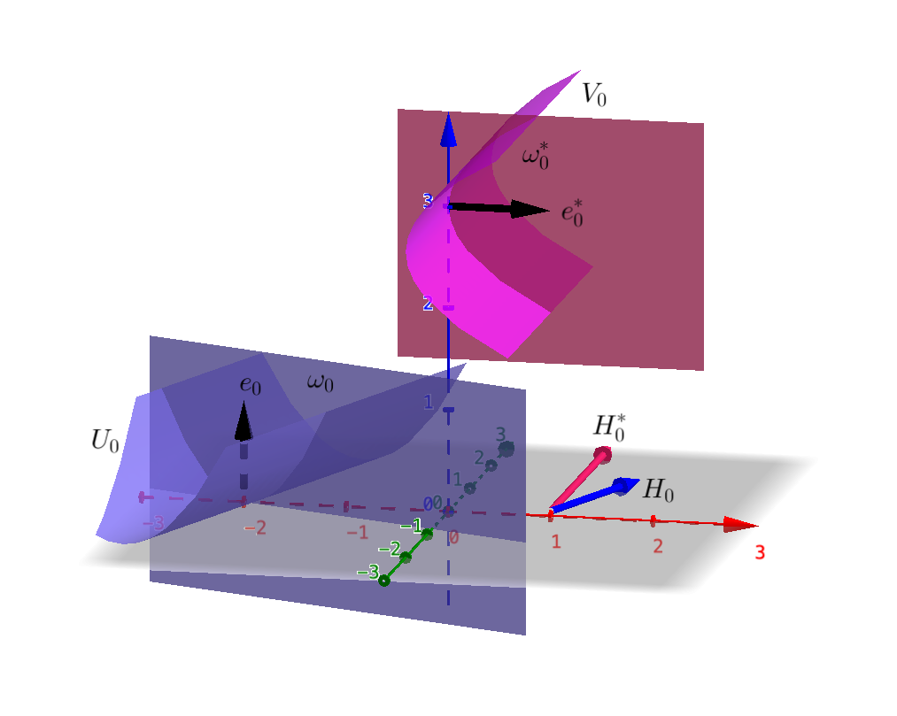
Fig. 5.4.

Lemma 5.14.

There exists an affine transformation $A$ with $\mbox{det}\,A=1$ such that $AH_{0}=(A^{t})^{-1}H_{0}^{*}$. Hence, by the affine transform $A$ and another coordinate change, we can make both $A(U_{0})$ and $(A^{t})^{-1}(V_{0})$ flat in the $e_{2},\cdots,e_{n-1}$ directions.

Proof.

We first claim that for any unit vector $e\in H_{0}$, $e$ cannot be parallel to $e_{0}^{*}$. For if not, then $e_{0}^{*}\in H_{0}$. Let $u_{0}$ be the Legendre transform of $v_{0},$ namely,

(5.89) $$u_{0}(x)=\sup_{y\in\mathbb{R}^{n}}\left\{x\cdot y-v_{0}(y)\right\}\quad\text{for}\ x\in\overline{U_{0}}.$$

By Lemma 5.12, we have that $u_{0}$ is strictly convex and $C^{1}$ in $B_{r_{0}}(0)\cap\overline{U_{0}}$ for some $r_{0}>0.$ Note that since $v_{0}(0)=0$, $v_{0}\geq 0$, we also have $u_{0}(0)=0$, $u_{0}\geq 0$. On the other hand, by (5.77) $Du_{0}(U_{0}\cap B_{r}(0))\subset\{y:y\cdot e_{0}^{*}\geq 0\}$, we have $Du_{0}\cdot e_{0}^{*}\geq 0$ in $U_{0}\cap B_{r}(0),$ namely $u_{0}$ is monotone increasing in the $e_{0}^{*}$ direction. It follows that $u_{0}(-te_{0}^{*})\leq 0$ for $t>0$ small, and thus $u_{0}(-te_{0}^{*})=0$ for $t>0$ small, which contradicts to the strict convexity of $u_{0}$. The claim is proved.

Now, for a fixed unit vector $e\in H_{0}$, by the above claim we can find a vector $\tilde{e}\in H_{0}^{*}$ such that $e$ is not orthogonal to $\tilde{e}$. Hence there exists an affine transformation $A_{1}$ with $\mbox{det}A_{1}=1$ such that $A_{1}e$ is parallel to $(A_{1}^{t})^{-1}\tilde{e}$ (see (3.2) and [8, (4.7)]). The unit inner normals of $A_{1}(U_{0})$ and $(A_{1}^{t})^{-1}V_{0}$ at $0$ are still orthogonal to each other. Denote $\bar{e}_{2}=\frac{A_{1}e}{|A_{1}e|}$. Then, $A_{1}(U_{0})=\omega_{1}\times H_{1}\times\text{span}\{\bar{e}_{2}\}$, where $\omega_{1}$ is a two dimensional convex subset and $H_{1}$ is an $n-3$ dimensional subspace in $\mathbb{R}^{n}$. Similarly, $(A_{1}^{t})^{-1}V_{0}=\omega^{*}_{1}\times H^{*}_{1}\times\text{span}\{\bar{e}_{2}\}$, where $\omega^{*}_{1}$ is a two dimensional convex subset and $H^{*}_{1}$ is an $n-3$ dimensional subspace in $\mathbb{R}^{n}$.

Then we restrict ourself to the sets $\omega_{1}\times H_{1}$ and $\omega^{*}_{1}\times H^{*}_{1}$ in the $(n-1)$-space $(\bar{e}_{2})^{\bot}$. Similarly as above, we can find unit vectors $e^{\prime}\in H_{1},\tilde{e}^{\prime}\in H^{*}_{1}$ and an affine transform $A_{2}$ such that $A_{2}e^{\prime}$ is parallel to $(A_{2}^{t})^{-1}\tilde{e}^{\prime}$, and $A_{2}\bar{e}_{2}=\bar{e}_{2}$ remains unchanged. Let $\bar{e}_{3}=\frac{A_{2}e^{\prime}}{|A_{2}e^{\prime}|}$. Repeating this process, after a sequence of affine transformations $A_{i}$, $i=1,\cdots,n-2$, we have $AH_{0}=(A^{t})^{-1}H_{0}^{*}$, where $A=A_{n-2}\cdots A_{1}.$ ∎

Proof of Proposition 5.1 when $n\geq 3$.

By Lemma 5.9, Lemma 5.11, Lemma 5.14 and the relation (5.88), up to an affine transformation and a change of coordinates we may assume $V_{0}=\omega_{0}^{*}\times H$ and $U_{0}=\omega_{0}\times H,$ where $H=\text{span}\{e_{2},\cdots,e_{n-1}\},$ and

(5.90) $$\omega_{0}^{*}=\{(y_{1},y_{n}):y_{1}\geq\rho_{0}^{*}(y_{n})\}$$

for some smooth convex function $\rho_{0}^{*}$ satisfying $\rho_{0}^{*}\geq 0$, $\rho_{0}^{*}(0)=0.$ Meanwhile, $\omega_{0}$ is a convex set in $\text{span}\{e_{1},e_{n}\}$ with $0\in\partial\omega_{0}$ and $\omega_{0}\subset\{(x_{1},x_{n}):x_{n}\geq 0\}.$ However, $\partial\omega_{0}$ may not be a graph of a function of $x_{1}$, for example see Fig. 5.5. To make $\partial\omega_{0}$ locally a graph, we can apply a sliding transform as follows.

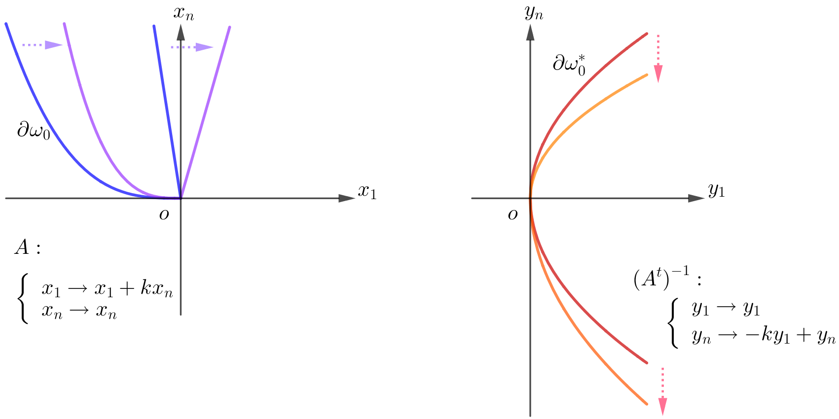
Fig. 5.5.

Let $A$ be an affine transform such that

$$A:\left\{\begin{array}[]{rll}x_{1}&\to\ \ x_{1}+kx_{n}&\text{for a constant $k\in\mathbb{R}$}\\ x_{i}&\to\ \ x_{i}&\text{for }i=2,\cdots,n.\end{array}\right.$$

Note that $A$ makes $U_{0}$ to slide along the $x_{1}$ direction, and at the same time $(A^{t})^{-1}$ makes $V_{0}$ slide along the $y_{n}$ direction, while the $(n-2)$-space $H$ remains invariant. Hence, by choosing a proper constant $k\in\mathbb{R}$, we may assume that $\omega_{0}=\{(x_{1},x_{n}):x_{n}\geq\rho_{0}(x_{1})\}$ for a convex function $\rho_{0}.$ Note that since $\rho_{0}^{*}$ is smooth, after the corresponding affine transform $(A^{t})^{-1},$ $\omega_{0}^{*}$ still satisfies (5.90) but with a different smooth function $\rho_{0}^{*}.$ ∎

Remark 5.5.

By the proof of Lemma 5.9, after the above transform, we have that $\partial V_{0}=\{y_{1}>P_{0}(y)\}$ for some nonnegative quadratic polynomial. Since $\partial V_{0}$ is flat in $e_{2},\cdots,e_{n-1}$ directions, we have that $P_{0}$ depends only on $y_{1},y_{n}.$ Since $P_{0}$ is nonnegative, we may denote it as $P_{0}(y)=ay_{n}^{2}+2by_{n}y_{1}+cy_{1}^{2}$ with $b^{2}\leq ac.$ We claim that $b=c=0$ and $a>0.$ In fact, if $c>0,$ then $P_{0}(te_{1})>y_{1}$ for $t$ large, which implies $te_{1}\notin V_{0}.$ On the other hand, by (5.61) we have that $te_{1}\in V_{0}$ for any $t$ large, which is a contradiction. Hence, $c=0,$ which also implies $b=0.$ If $a=0,$ then $\partial V_{0}$ is flat, which implies that $te_{n}\in\partial V_{0}$ for $t<0.$ Since $Dv_{0}(\mathbb{R}^{n})\subset\{x:x_{n}\geq 0\},$ which implies that $v_{0}$ is increasing in $e_{n}$ direction. Since $v_{0}\geq 0$ and $v_{0}(0)=0,$ it implies that $v_{0}(te_{n})=0$ for all $t<0,$ contradicting to the strict convexity of $v_{0}$ in $B_{1}(0)\cap\overline{V_{0}}.$ Therefore, we may denote $\partial V_{0}:=\{y:y_{1}=\rho^{*}_{0}(y_{n})\}$ with $\rho^{*}_{0}(y_{n})=ay_{n}^{2}$ for some positive constant $a.$

6. Proof of obliqueness

In this section we will use the limit profile obtained in Section 5 to prove the following obliqueness estimate.

Proposition 6.1.

Assume that $\overline{\Omega},\overline{\Omega^{*}}\subset\mathbb{R}^{n}$ are disjoint, uniformly convex domains with $C^{2}$ boundaries, and that the densities $f\in C({\overline{\Omega}})$, $g\in C(\overline{\Omega^{*}})$ are positive, continuous functions. Then for any $x_{0}\in\mathcal{F}$ and $y_{0}=Du(x_{0})$, we have

(6.1) $$\nu_{{}_{U}}(x_{0})\cdot\nu_{{}_{V}}(y_{0})>0,$$

where $\nu_{{}_{U}}(x_{0})$ is the unit inner normal of $U$ at $x_{0}$, and $\nu_{{}_{V}}(y_{0})$ is the unit inner normal of $V$ at $y_{0}$.

6.1. Obliqueness in dimension two

In the argument below, we will adopt some techniques from [6]. Recall that if the obliqueness fails at $x_{0},$ then Proposition 5.1 holds. Let $v_{0},U_{0},V_{0}$ be as in Proposition 5.1:

(6.2) $$V_{0}=\big{\{}(y_{1},y_{2})\in\mathbb{R}^{2}\,:\,y_{1}>\rho_{0}^{*}(y_{2})\big{\}},$$

where $\rho_{0}^{*}(t)=at^{2}$ for some constant $a>0$, and

(6.3) $$U_{0}=\big{\{}(x_{1},x_{2})\in\mathbb{R}^{2}\,:\,x_{2}>\rho_{0}(x_{1})\big{\}},$$

where $\rho_{0}$ is a convex function satisfying $0\leq\rho_{0}(t)\leq Ct^{2}$ for a constant $C>0$, and $\rho_{0}(t)=\frac{1}{2r}t^{2}$ for $t<0$, where $r>0$ is a constant. By subtracting a constant we may assume that $v_{0}(0)=0.$

Recall that by (5.82), we have that $Dv_{0}(\partial V_{0}\cap B_{r^{\prime}}(0))\subset\partial U_{0}.$ Then by the monotonicity of convex function $v_{0}$ we have

(6.4) $$Dv_{0}(y)\in\partial U_{0}\cap\{x_{1}<0\}\quad\ \forall\,y\in\partial V_{0}\cap\{y_{2}>0\}\cap B_{r^{\prime}}(0).$$

Indeed, given any $y\in\partial V_{0}\cap\{y_{2}>0\}\cap B_{r^{\prime}}(0),$ suppose $x=Dv_{0}(y)\in\partial U_{0}\cap\{x_{1}\geq 0\}.$ Let $\{\tilde{x}\in\mathbb{R}^{2}:(\tilde{x}-x)\cdot e=0\}$ be a supporting line of the convex set $U_{0}$ at $x\in\partial U_{0},$ for some unit vector $e.$ Replacing $e$ by $-e$ if necessary, we may also assume that $U_{0}\subset\{\tilde{x}\in\mathbb{R}^{2}:(\tilde{x}-x)\cdot e>0\}.$ Note that $e$ can be chosen as the unit inner normal vector of $\partial U_{0}$ at $x$ when $\partial U_{0}$ is $C^{1}$ at $x.$ Then, by (6.2), (6.3) and using the assumptions that $y_{2}>0$ and $x_{1}\geq 0,$ we have that the angle between $e$ and the unit inner normal of $V_{0}$ at $y$ is strictly large than $\frac{\pi}{2}.$ Hence, by the smoothness of $\partial V_{0}$ we have that $-e$ points inside $V_{0},$ namely $y-te\in V_{0}$ for $t>0$ small. Denote $x_{t}:=Dv_{0}(y-te)\in U_{0}\subset\{\tilde{x}\in\mathbb{R}^{2}:(\tilde{x}-x)\cdot e>0\}.$ Then,

$$\left(Dv_{0}(y-te)-Dv_{0}(y)\right)\cdot(y-te-y)=(x_{t}-x)\cdot(-e)<0,$$

contradicting to the monotonicity of $Dv_{0}.$

By ($i$) of Proposition 5.1, we have that both $\partial U_{0}\cap\{x_{1}<0\}$ and $\partial V_{0}\cap\{y_{2}>0\}$ are smooth and uniformly convex. Hence by the localised estimates of Caffarelli [4], $v_{0}$ is smooth up to the boundary in $V_{0}\cap\{y_{2}>0\}$. Let $p,\xi$ be the points on $\partial S_{h}[v_{0}]$ such that

(6.5) $$p_{2}=p\cdot e_{2} =\sup\{y\cdot e_{2}\,:\,y\in S_{h}[v_{0}]\},$$

$$\xi_{2}=\xi\cdot e_{2} =\inf\{y\cdot e_{2}\,:\,y\in S_{h}[v_{0}]\}.$$

From (6.4), one sees that $p$ is in the interior of $V_{0}$. Hence $\{x\in\mathbb{R}^{2}:x_{2}=p_{2}\}$ is the tangent line of $\{v_{0}<h\}$ at $p.$ We claim that

(6.6) $$p_{2}\geq C|\xi_{2}|$$

for a constant $C>0$ independent of $h$. The proof of (6.6) is similar to that of [6, Lemma 4.1]. For the reader’s convenience, we include a brief proof below.

Suppose (6.6) is not true, then there exists a sequence $h\rightarrow 0$ such that

(6.7) $$\frac{p_{2}}{\xi_{2}}\rightarrow 0\quad\text{as }\ h\rightarrow 0.$$

Let $T_{h}$ be a linear transformation such that $T_{h}(S_{h}[v_{0}])\sim B_{1}$, and let $v_{0h}(\cdot)=\frac{1}{h}v_{0}(T_{h}^{-1}(\cdot)).$ Similarly to $v_{h}$, $v_{0h}$ sub-converges to a convex function $\bar{v}$ locally uniformly as $h\to 0$. Denote $H_{1h}=T_{h}\left(\{x_{2}=p_{2}\}\right)$ and $H_{2h}=T_{h}\left(\{x_{2}=\xi_{2}\}\right).$ By (6.7) we have

$$\frac{\text{dist}(0,H_{1h})}{\text{dist}(0,H_{2h})}\rightarrow 0\quad\text{as }\ h\rightarrow 0.$$

Along a subsequence, $H_{1h}$ and $H_{2h}$ converge to straight lines $H_{1}$ and $H_{2}$, respectively. Since $T_{h}(S_{h}[v_{0}])$ has a good shape, we have $\text{dist}(H_{1h},H_{2h})\approx 1$. Then the limit $H_{1}$ passes $0$. On the other hand, since $H_{1h}$ is a tangent line of $\{v_{0h}=1\}$, we have $v_{0h}\geq 1$ on one side of $H_{1h}$. Passing to the limit, we have $\bar{v}\geq 1$ on one side of $H_{1}$, which however contradicts to the facts that $0\in H_{1}$, $\bar{v}(0)=0$ and $\bar{v}$ is continuous. Hence claim (6.6) is proved.

Recall that $Dv_{0}(V_{0})\subset\{x_{2}\geq 0\}$. Hence $v_{0}$ is increasing in $y_{2}$, and $\sup\{y\cdot e_{1}:y\in S_{h}[v_{0}]\}$ is achieved at $\xi$, the point defined in (6.5). That is

$$\xi_{1}=\sup\{y\cdot e_{1}\,:\,y\in S_{h}[v_{0}]\}.$$

From (2.28), (6.6) and noting that $\xi\in\partial V_{0}=\{y_{1}=ay_{2}^{2}\}$, we have the estimates

$$h\approx|S_{h}[v_{0}]| \leq Cp_{2}\xi_{1}$$

$$\leq Cp_{2}\xi_{2}^{2}\leq Cp_{2}^{3}.$$

It implies that $p_{2}\gtrsim h^{1/3}$. Therefore, as $p\in\partial S_{h}[v_{0}]$, we obtain

$$v_{0}(p)=h\leq Cp_{2}^{3}.$$

Denote $\tilde{p}=(p_{1},\frac{1}{2}p_{2}).$ Since $v_{0}$ is increasing in the $e_{2}$ direction, we have $v_{0}(\tilde{p})\leq v_{0}(p)$ and

(6.8) $$v_{0}(\tilde{p})\leq h\leq Cp_{2}^{3}.$$

By the convexity of $v_{0}$,

(6.9) $$\partial_{2}v_{0}(\tilde{p})\leq\frac{v_{0}(p)-v_{0}(\tilde{p})}{\frac{1}{2}p_{2}}\leq C\frac{h}{p_{2}}\leq Cp_{2}^{2},$$

where $\partial_{2}v_{0}=\partial_{y_{2}}v_{0}\geq 0$.

Introduce the function

(6.10) $$w(y):=\partial_{2}v_{0}(y)+v_{0}(y)-y_{2}\partial_{2}v_{0}(y)\quad\mbox{ in }V_{0}.$$

By equation (5.18), $w$ satisfies

$$\sum_{i,j=1}^{2}V^{ij}w_{ij}=0\ \ \ \text{ in }V_{0},$$

where $\{V^{ij}\}$ is the cofactor matrix of $\{D^{2}v_{0}\}$.

Lemma 6.1.

Let

(6.11) $$\underline{w}(t):=\inf\big{\{}w(y_{1},t)\,:\,y_{1}>\rho_{0}^{*}(t)\big{\}},\quad 0<t<1.$$

Then for $t>0$ small, say $t\in(0,\delta_{0})$, we have

(6.12) $$0\leq\underline{w}(t)\leq Ct^{2}.$$

Proof.

Observe that $w=(1-y_{2})\partial_{2}v_{0}+v_{0}\geq 0$ for $y_{2}<1.$ Let $p$ be the point defined in (6.5). By (6.8) and (6.9), we have

$$\underline{w}(\frac{1}{2}p_{2})\leq w(\tilde{p})\leq Cp_{2}^{3}+Cp_{2}^{2}\leq 2Cp_{2}^{2},$$

for $p_{2}>0$ small. By sending $h\rightarrow 0,$ $p_{2}$ will take all arbitrarily small positive values, hence the desired estimate follows. ∎

Lemma 6.2.

For $t>0$ small, the minimum of $w(\cdot,t)$ in (6.11) is attained in the interior of $V_{0}.$

Proof.

Recall that $v_{0}$ is smooth up to the boundary in $V_{0}\cap\{y_{2}>0\},$ and

$$\partial V_{0}\cap\{y_{2}>0\}=\left\{(y_{1},y_{2})\,:\,y_{1}=\rho_{0}^{*}(y_{2})=ay_{2}^{2},\ y_{2}>0\right\}.$$

For $y=(y_{1},y_{2})\in\partial V_{0}\cap\{y_{2}>0\}$, by (6.4) and (5.22), we have

$$Dv_{0}(y)\in\Big{\{}(x_{1},x_{2})\,:\,x_{2}=\rho_{0}(x_{1})=\frac{1}{2r}x_{1}^{2},\ x_{1}<0\Big{\}}.$$

Hence

$$\partial_{2}v_{0}(\rho_{0}^{*}(t),t)=\rho_{0}(\partial_{1}v_{0}(\rho_{0}^{*}(t),t))\quad\ \text{ for }\ t>0.$$

Differentiating the above equation in $t$, we obtain

$$\partial_{21}v_{0}\cdot\left((\rho_{0}^{*})^{\prime}-\rho_{0}^{\prime}\right)=\rho^{\prime}_{0}(\rho_{0}^{*})^{\prime}\partial_{11}v_{0}-\partial_{22}v_{0}.$$

Since $(\rho_{0}^{*}(t))^{\prime}>0$, $\rho_{0}^{\prime}(\partial_{1}v_{0}(\rho_{0}^{*}(t),t))<0$ for $t>0$, and $\partial_{11}v_{0}>0$, $\partial_{22}v_{0}>0$, from the above formula it follows that $\partial_{21}v_{0}<0$ for $t>0$. Hence for $y=(\rho_{0}^{*}(y_{2}),y_{2})\in\partial V_{0}$ with $0<y_{2}<1$, we obtain

$$\partial_{1}w(y)=(1-y_{2})\partial_{21}v_{0}+\partial_{1}v_{0}<0.$$

On the other hand, recall that $\partial_{2}v_{0}\geq 0$ and $v_{0}\geq 0$. For any small $\delta>0$, by the strict convexity of $v_{0}$ in $V_{0}$, there exists $\epsilon>0$ such that

$$w(y)=(1-y_{2})\partial_{2}v_{0}+v_{0}\geq\epsilon\ \ \ \text{for}\ y\in B_{1}(0)\backslash B_{\delta}.$$

By the assumption in the beginning of Section 5, we have that $v(0)=0,v\geq 0,$ which implies that $v_{h}(0)=0,v_{h}\geq 0,$ passing to limit $h\rightarrow 0,$ we have $v_{0}(0)=0,v_{0}\geq 0.$ Hence $Dv_{0}(0)=0.$ Note that by Lemma 5.12, we have that $v_{0},$ as a convex function defined on $\mathbb{R}^{n},$ is differentiable at $0.$ By the definition of $w,$ we have $w(0)=\partial_{2}v_{0}(0)+v_{0}(0)-y_{2}\partial_{2}v_{0}(0)=0.$ Hence, by the $C^{1}$ regularity of $v_{0}$, there exists $\delta_{0}>0$, such that $w(\cdot,t)$ attains its minimum in the interior of $V_{0}$ for any $0<t<\delta_{0}.$ ∎

Lemma 6.3.

For $t\in(0,\delta_{0})$, the function $\underline{w}$ defined in (6.11) is concave,

Proof.

If $\underline{w}$ is not concave, there exist constants $0<r_{1}<r_{2}<\delta_{0}$ and an affine function $L(t)$ such that $\underline{w}(r_{i})=L(r_{i})$ for $i=1,2$, and the set $\{t\in(r_{1},r_{2}):w(t)<L(t)\}\neq\emptyset$. Extend $L$ to $\mathbb{R}^{2}$ such that $L(s,t)=L(t)$, namely, $L$ is independent of $s$. Denote

$$D_{\varepsilon}=\{y\in V_{0}\ :\ y_{2}\in(r_{1},r_{2}),\text{ and }w(y)<L(y)-\varepsilon\}.$$

By our definition of $\underline{w}$ and Lemma 6.2, we can choose $\varepsilon>0$ such that

(6.13) $$\emptyset\neq D_{\varepsilon}\Subset V_{0}.$$

Indeed, by our choice of $L$, $D_{\varepsilon\,|\,\varepsilon=0}\neq\emptyset$. Let $\varepsilon_{0}=\sup\{\varepsilon\,:\,D_{\varepsilon}\neq\emptyset\}$. Then (6.13) holds for $\varepsilon<\varepsilon_{0}$ and sufficiently close to $\varepsilon_{0}$.

Recall that $\sum_{i,j}V^{ij}w_{ij}=0$ in $V_{0}$. The strong maximum principle implies that $w=L$ in $D_{\varepsilon}$. However, $w<L$ in $D_{\varepsilon}$ by our definition of $D_{\varepsilon}$. We reach a contradiction. ∎

Proof of Proposition 6.1 in 2d.

Suppose the obliqueness fails. By Lemma 6.1 and Lemma 6.3, $\underline{w}(t)$ is concave in $(0,\delta_{0})$ and satisfies $0\leq\underline{w}(t)\leq Ct^{2}$. Note that $\underline{w}(t)\to 0$ as $t\to 0$. Hence, we must have $\underline{w}(t)\equiv 0$ for $t\in(0,\delta_{0})$. On the other hand, for a fixed $t_{0}\in(0,\delta_{0})$, by the strict convexity of $v_{0}$, we have $w(y_{1},t_{0})=(1-t_{0})\partial_{2}v_{0}+v_{0}>\epsilon_{0}$ for any $(y_{1},t_{0})\in\overline{V_{0}}$, where the constant $\epsilon_{0}>0$ is independent of $y_{1}$. Therefore, $\underline{w}(t_{0})\geq\epsilon_{0}>0$. We reach a contradiction. ∎

6.2. Obliqueness in higher dimensions

Suppose the obliqueness fails at $x_{0},$ let $v_{0},U_{0},V_{0}$ be as in Proposition 5.1. When $n\geq 3,$ since $U_{0}$ is not $C^{1,1}$ in general, we do not have the $C^{2}$ regularity of $v_{0}$ up to $\partial V_{0}\cap\{y_{n}>0\}$ as that in dimension 2. Hence, in the proof we need to use the approximation technique developed in [6, Section 5.2].

Proof of Proposition 6.1 for general dimensions.

Step 1. By Proposition 5.1, we may assume that

(6.14) $$\partial U_{0} =\{x:x_{n}=\rho_{0}(x_{1})\};$$

$$\partial V_{0} =\{y:y_{1}=\rho_{0}^{*}(y_{n})\}$$

for a convex function $\rho_{0}$ satisfying $\rho_{0}(0)=0$, $\rho_{0}\geq 0$; and for a smooth convex function $\rho_{0}^{*}$ satisfying $\rho_{0}^{*}(0)=0$, $\rho_{0}^{*}\geq 0$.

We remark that the smoothness of $\rho_{0}^{*}$ follows from Lemma 5.9, but the function $\rho_{0}$ may not be smooth. Unlike (5.22) in dimension two, the lack of smoothness of $\rho_{0}$ prevents us from obtaining further regularity of $v_{0}$. By (5.45), $v_{0}$ satisfies

(6.15) $$\mbox{det}\,D^{2}v_{0}=c_{0}\chi_{{}_{V_{0}}}\ \ \text{in}\ \mathbb{R}^{n},$$

$$Dv_{0}(V_{0})=U_{0}$$

for a constant $c_{0}>0$. To overcome this obstacle, in the following we first show that $v_{0}$ can be approximated by a sequence of smooth functions.

Fix a small $r_{0}>0$, let $\tilde{V}_{0}$ be interior of the convex hull of $\Sigma:=Du_{0}(B_{r_{0}}\cap\overline{U_{0}})$, where $u_{0}$ is as in (5.89). By the proof of Lemma 5.12, in particular (5.77) and (5.81), we have that

(6.16) $$B_{\delta}(0)\cap\overline{V_{0}}\subset\Sigma\subset\overline{V_{0}},$$

for $\delta$ small. Now, by (6.16) and convexity of $V_{0},$ when we take convex hull of $\Sigma,$ the part $B_{\delta}(0)\cap\overline{V_{0}}$ is not changed. Therefore, we have that

(6.17) $$\tilde{V}_{0}\cap B_{\delta}(0)=\Sigma\cap B_{\delta}(0)=V_{0}\cap B_{\delta}(0)$$

when $\delta>0$ is small.

Approximating $\rho_{0}$ by smooth convex functions $\rho_{k},$ we can approximate $B_{r_{0}}\cap U_{0}$ in Hausdorff distance by a sequence of convex set $U_{k}:=\{x:\ x_{n}>\rho_{k}(x_{1})\}\cap B_{r_{0}}$, which is smooth near $0$, such that for each $k$,

$$\partial U_{k}\cap B_{r_{0}}=\{x\,:\,x_{n}=\rho_{k}(x_{1})\}$$

for a convex, smooth function $\rho_{k}$ satisfying $\rho_{k}(0)=0$, $\rho_{k}\geq 0$, and $\rho_{k}^{\prime}(t)<0$ when $t<0$; and such that $\rho_{k}\to\rho_{0}$ locally uniformly as $k\to\infty$. Now, let $v_{k}$ be the convex function solving

$$(Dv_{k})_{\#}(c_{k}\chi_{{}_{\Sigma}}+\frac{c_{k}}{k}\chi_{{}_{\tilde{V}_{0}\backslash\Sigma}})=\chi_{{}_{U_{k}}},$$

where the constant

$$c_{k}=\frac{|U_{k}|}{|\Sigma|+\frac{1}{k}|\tilde{V}_{0}\backslash\Sigma|}\rightarrow c_{0}\ \ \text{as}\ k\rightarrow\infty.$$

By the definition of $U_{k}$ and the fact that the convex fucntions $\rho_{k}\to\rho_{0}$ locally uniformly as $k\to\infty,$ we can deduce that $|U_{k}|$ converges to $|B_{r_{0}}\cap U_{0}|.$

Then by (6.17) and subtracting a constant if necessary, we have that $v_{k}\rightarrow v_{0}$ uniformly in $B_{r_{1}}(0)\cap\overline{V_{0}}$ as $k\rightarrow\infty$, for some $r_{1}<r_{0}$ independent of $k$.

We also extend $v_{k}$ to $\mathbb{R}^{n}$ as follows

$$v_{k}(x):=\sup\{L(x)\,:\,L\ \text{is affine},L\leq v_{k}\ \text{in}\ \tilde{V}_{0},\ \text{and}\ DL\in U_{k}\}$$

for any $x\in\mathbb{R}^{n}.$ By subtracting a constant, we may assume $v_{k}(0)=0.$ Since

$$\|Dv_{k}\|_{L^{\infty}(\mathbb{R}^{n})}\leq\text{diam}(U_{k})\leq r_{0},$$

up to a subsequence, we may assume $v_{k}$ converges to a convex function $\tilde{v}_{0}$ locally uniformly. Now, by weak convergence of Monge-Ampère measure we have $\mbox{det}D^{2}\tilde{v}_{0}=c_{0}\chi_{\Sigma}$ in $\mathbb{R}^{n}.$ Moreover, $D\tilde{v}_{0}$ is the optimal map from $\Sigma$ to $B_{r_{0}}(0)\cap U_{0}.$ By uniqueness of optimal maps we have that $\tilde{v}_{0}=v_{0}$ in $V_{0}\cap B_{\delta}(0).$ Since $v_{0}$ is differentiable at $0$ (follows from Lemma 5.12), we have that $\partial v_{0}(B_{\delta}(0))\subset B_{r_{0}}(0)\cap\overline{U_{0}},$ provided $\delta$ is small enough. This implies that $v_{0}=\tilde{v}_{0}$ in $B_{\delta}(0).$ Since $v_{k}\rightarrow v_{0}$ uniformly in $B_{\delta}(0)$ and $v_{0}$ is differentiable at points in $B_{\delta}(0)\cap\overline{V_{0}}$ (follows from Lemma 5.12), by the argument in Remark 5.4, we have that $Dv_{k}$ converges to $Dv_{0}$ uniformly in $B_{r_{1}}(0)\cap\overline{V_{0}}$ by choosing $r_{1}=\frac{\delta}{2}.$

Since $\partial U_{k},\partial\tilde{V}_{0}$ are also smooth near $0,$ by the localised $C^{2,\alpha}$ estimate in [6, Theorem 1.1], $v_{k}$ is smooth in $B_{r_{2}}\cap\overline{V_{0}}$, for some $r_{2}>0$ independent of $k$. Here $r_{2}<r_{1}$ is chosen small such that $Dv_{k}(B_{r_{2}}\cap\overline{V_{0}})\subset B_{\frac{r_{0}}{2}}(0)\cap\overline{U_{k}}.$ Since $Dv_{k}$ converges to $Dv_{0}$ uniformly in $B_{r_{1}}(0)\cap\overline{V_{0}},$ $v_{0}\in C^{1}(B_{r_{1}}(0)\cap\overline{V_{0}})$ and $Dv_{0}(0)=0,$ we can choose such $r_{2}$ uniformly for all $k.$ Note that the statement of [6, Theorem 1.1] is a global one, but the proof is actually a local one. Indeed, for any $y\in B_{r_{2}}\cap\partial V_{0},$ by the above discussion we have that $Dv_{k}(y)\in B_{\frac{r_{0}}{2}}(0)\cap\partial U_{k}.$ Since both $B_{r_{2}}\cap\partial V_{0}$ and $B_{\frac{r_{0}}{2}}(0)\cap\partial U_{k}$ are smooth, and densities are positive constants in $B_{r_{2}}\cap\overline{V_{0}}$ and $B_{\frac{r_{0}}{2}}(0)\cap\overline{U_{k}},$ by [6, Lemma 3.1] we have the tangential $C^{1,1-\epsilon}$ estimate of $u_{k}$ holds at $y,$ then, by [6, Section 5] we have that the obliqueness holds at points $y$ and $Dv_{k}(y).$ Finally by [6, proof of Theorem 1.1, Section 6], we have that $v_{k}$ is $C^{2,\alpha}$ smooth at $y.$ Therefore we obtain a smooth approximation sequence of $v_{0}$. Note that we only need to use the smoothness of $v_{k}$ in $B_{r_{2}}\cap\overline{V_{0}}$ for taking the second order derivative, but we do not need to use the bound of $C^{2}$ norm for $v_{k}.$

Step 2. Let $w(y):=\partial_{n}v_{0}(y)+v_{0}(y)-\frac{n}{2}y_{n}\partial_{n}v_{0}(y)$, and define

$$\underline{w}(t)=\inf\{w(y_{1},y_{2},\cdots,y_{n-1},t)\,:\,y_{1}>\rho_{0}^{*}(t)\},\quad 0<t<1.$$

Replacing $v_{0}$ by $v_{k}$, we can also define $w_{k}$ and $\underline{w_{k}}$ in the same way. Note that for a point $y=(\rho_{0}^{*}(y_{n}),y_{2},\cdots,y_{n})\in\partial V_{0}\cap B_{\delta}(0)$ with $y_{n}>0,$ we have that $x=Dv_{k}(y)\in\partial U_{k}.$ Similar to the reason for (6.4), we also have that $x_{1}<0.$ By the definition of $U_{k},$ we have that $x_{n}=\rho_{k}(x_{1}),$ hence,

$$\partial_{n}v_{k}(\rho_{0}^{*}(y_{n}),y_{2},\cdots,y_{n})=\rho_{k}\left(\partial_{1}v_{k}(\rho_{0}^{*}(y_{n}),y_{2},\cdots,y_{n})\right).$$

Then similar to the computation in Lemma 6.2, we can show that $\partial_{n1}v_{k}(y)<0.$ Now, analogously to Lemmas 6.2 and 6.3, one can verify that $\underline{w_{k}}(t)$ is a concave function in $(0,\delta_{0})$ for some positive constant $\delta_{0}$ independent of $k$. Hence by passing to the limit, $\underline{w}(t)$ is also concave in $(0,\delta_{0})$.

Denote $\hat{U}_{0}=Dv_{0}(B_{1}(0)\cap V_{0}).$ By the strict convexity of $v_{0}$ in $\overline{V_{0}},$ we have $B_{r_{1}}(0)\cap U_{0}\subset\hat{U}_{0}$ for some small $r_{1}>0$. Hence $\hat{U}_{0}$ is locally convex near 0. Let

$$\tilde{u}_{0}(x):=\sup\{L(x):L\ \text{is affine},\ L\leq u_{0}\ \text{in}\ \hat{U}_{0},\ \text{and}\ DL\in B_{1}(0)\cap V_{0}\},\ \ \ x\in\mathbb{R}^{n},$$

where $u_{0}$ is the Legendre transform of $v_{0}$ as in (5.89). Then $\tilde{u}_{0}$ satisfies

(6.18) $$\mbox{det}\,D^{2}\tilde{u}_{0}=\frac{1}{c_{0}}\chi_{\hat{U}_{0}}\ \ \ \text{in}\ \mathbb{R}^{n}.$$

Since $\tilde{u}_{0}$ is strictly convex in $\overline{\hat{U}_{0}}$, and $B_{r_{1}}(0)\cap U_{0}\subset\hat{U}_{0}$, we have $S^{c}_{h}[\tilde{u}_{0}]\cap U_{0}=S^{c}_{h}[\tilde{u}_{0}]\cap\hat{U}_{0}$ for $h$ small.

Since $U_{0}$ is flat in $e_{2},\cdots,e_{n-1}$ directions near $0$, the right hand side of (6.18) is independent of $x_{2},\cdots,x_{n-1}$ near $0$. By Pogorelov’s interior second derivative estimate (see [4, Corollary 1.1]), $\tilde{u}_{0}$ is $C^{1,1}$ smooth in the $e_{i}$-direction near $0$, for $i=2,\cdots,n-1$. Namely, $u_{0}(te_{i})=\tilde{u}_{0}(te_{i})\leq C_{1}t^{2}$ near $t=0$. Hence, for $i=2,\cdots,n-1$ and $y\in V_{0}$ close to $0$,

$$v_{0}(y) =u_{0}^{*}(y)$$

$$=\sup_{x\in\overline{U_{0}}}\left\{x\cdot y-u_{0}(x)\right\}$$

$$\geq\sup_{t\in(-1,1)}\left\{te_{i}\cdot y-C_{1}t^{2}\right\}$$

$$\geq C_{2}y_{i}^{2}$$

for a constant $C_{2}>0$. Hence

(6.19) $$S_{h}[v_{0}]\subset\left\{y\in\mathbb{R}^{n}\,:\,|y_{i}|\leq Ch^{\frac{1}{2}},\ i=2,\cdots,n-1\right\}$$

for some constant $C$ independent of $h.$

Step 3. We introduce the points $p,\xi,q\in\partial S_{h}[v_{0}]$ such that

$$p_{n} =\sup\{y_{n}\,:\,y\in S_{h}[v_{0}]\},$$

$$\xi_{n} =\inf\{y_{n}\,:\,y\in S_{h}[v_{0}]\},$$

$$q_{1} =\sup\{y_{1}\,:\,y\in S_{h}[v_{0}]\}.$$

Similarly to the proof of (6.6) (see also [6, Corollary 5.1]), we have $p_{n}\geq C|\xi_{n}|.$ By (6.19), $S_{h}[v_{0}]$ is contained in a cuboid, that is

(6.20) $$S_{h}[v_{0}]\subset[0,q_{1}]\times[-Ch^{\frac{1}{2}},Ch^{\frac{1}{2}}]^{n-2}\times[-Cp_{n},Cp_{n}].$$

Since $Dv_{0}(V_{0})\subset\{x_{n}\geq 0\}$, the function $v_{0}$ is monotone increasing in the $e_{n}$-direction, which implies $q\in\partial V_{0}$. Hence, from (6.14),

$$q_{1}=\rho_{0}^{*}(q_{n})\leq Cq_{n}^{2}\leq Cp_{n}^{2}.$$

From (6.20) and the volume estimate (2.28), we have

$$h^{\frac{n}{2}}\approx|S_{h}[v_{0}]|\leq Ch^{\frac{1}{2}(n-2)}p_{n}q_{1}\leq Ch^{\frac{1}{2}(n-2)}p_{n}^{3},$$

which implies $p_{n}\geq Ch^{1/3}$. It then follows, analogously to (6.8),

$$v_{0}(p)=h\leq Cp_{n}^{3}.$$

By following the proof of Lemma 6.1, we can further deduce the decay estimate

(6.21) $$0\leq\underline{w}(t)\leq Ct^{2}.$$

Step 4. In the above we have shown that $\underline{w}$ is concave and satisfies the estimate (6.21). We can now derive a contradiction as in dimension two, by showing that $\underline{w}$ is positive when $t>0$. On the one hand, by (6.21) and the concavity of $\underline{w}(t)$, we have $\underline{w}(t)\leq 0$ $\forall\,t\in(0,\delta_{0}).$ On the other hand, for a fixed $0<t_{0}<\delta_{0}$ small, by the strict convexity of $v_{0}$, we have

$$\underline{w}(y_{1},y_{2},\cdots,y_{n-1},t_{0})=(1-\frac{n}{2}t_{0})\partial_{n}v_{0}+v_{0}\geq\epsilon_{0},$$

where the constant $\epsilon_{0}>0$ is independent of $y_{1},\cdots,y_{n-1}$. Therefore, $\underline{w}(t_{0})\geq\epsilon_{0}>0$, which is a contradiction. ∎

References

- [1] E. Andriyanova and S. Chen. Boundary regularity of potential functions in optimal transportation with quadratic cost. Analysis and PDE 9 (2016),1483–-1496.
- [2] L. A. Caffarelli, The regularity of mappings with a convex potential. J. Amer. Math. Soc., 5 (1992), 99–104.
- [3] L. A. Caffarelli, Boundary regularity of maps with convex potentials. Comm. Pure Appl. Math., 45 (1992), 1141–1151.
- [4] L. A. Caffarelli, Boundary regularity of maps with convex potentials II. Ann. of Math., 144 (1996), 453–496.
- [5] L. A. Caffarelli and R. J. McCann, Free boundaries in optimal transport and Monge-Ampère obstacle problems. Ann. of Math., 171 (2010), 673–730.
- [6] S. Chen; J. Liu and X.-J. Wang, Global regularity for the Monge-Ampère equation with natural boundary condition. Ann. of Math., to appear.
- [7] S. Chen; J. Liu and X.-J. Wang, Boundary regularity for the second boundary-value problem of Monge-Ampère equations in dimension two, arXiv:1806.09482.
- [8] S. Chen and X.-J. Wang, Strict convexity and regularity of potential functions in optimal transportation under condition A3w. J. Differential Equations, 260 (2016),1954–1974,
- [9] Ph. Delanoë, Classical solvability in dimension two of the second boundary value problem associated with the Monge-Ampère operator. Ann. Inst. Henri Poincaré, Analyse Non Linéaire, 8 (1991), 443–457.
- [10] A. Figalli, A note on the regularity of the free boundaries in the optimal partial transport problem. Rend. Circ. Mat. Palermo, 58 (2009), 283-286.
- [11] A. Figalli, The optimal partial transport problem. Arch. Ration. Mech. Anal., 195 (2010), 533–560.
- [12] A. Figalli, The Monge-Ampère equation and its applications, Zurich Lectures in Advanced Mathematics, European Mathematical Society, 2017.
- [13] D. Gilbarg and N. S. Trudinger. Elliptic partial differential equations of second order. Springer-Verlag, Berlin, 2001.
- [14] E. Indrei, Free boundary regularity in the optimal partial transport problem. J. Funct. Anal., 264 (2013), 2497–2528.
- [15] H. Y. Jian and X.-J. Wang, Continuity estimates for the Monge-Ampère equation, SIAM J. Math. Anal., 39 (2007), 608–626.
- [16] J. Kitagawa and B. Pass. The multi-marginal optimal partial transport problem. In Forum of Mathematics, Sigma, volume 3. Cambridge University Press, 2015
- [17] J. Kitagawa and R. McCann, Free discontinuties in optimal transport. Arch. Rational Mech. Anal., 232 (2019), 1505–1541
- [18] O. Savin and H. Yu, Regularity of optimal transport between planar convex domains, available at Duke Math. J., 169 (2020), 1305–1327.
- [19] J. Urbas, On the second boundary value problem of Monge-Ampère type. J. Reine Angew. Math., 487 (1997), 115–124.
- [20] J. Urbas, Oblique boundary value problems for equations of Monge-Ampère type. Calc. Var. PDEs, 7 (1998), 19–39.
- [21] C. Villani, Topics in optimal transportation, Grad. Stud. Math. 58, Amer. Math. Soc., 2003.
- [22] C. Villani, Optimal transport, Old and new. Springer, Berlin, 2006.