Design of Anti-Jamming Waveforms for
Time-Hopping Spread Spectrum Systems in
Tone Jamming Environments

Abstract

We consider the problem of designing waveforms for mitigating single tone jamming (STJ) signals with an estimated jamming frequency in time-hopping spread spectrum (TH SS) systems. The proposed design of waveforms optimizes the anti-jamming (AJ) performance of TH SS systems by minimizing the correlation between the template and STJ signals, in which the problem of waveform optimization is simplified by employing a finite number of rectangular pulses. The simplification eventually makes the design of waveforms be converted into a problem of finding eigenvalues and eigenvectors of a matrix. Simulation results show that the waveforms designed by the proposed scheme provide us with performance superior not only to the conventional waveforms but also to the clipper receiver in the mitigation of STJ. The waveforms from the proposed design also exhibit a desirable AJ capability even when the estimated frequency of the STJ is not perfect.

I Introduction

The spread spectrum (SS) techniques, spreading the bandwidth of a signal beyond that actually required, have been developed not only for commercial communication but also for covert communication. Systems adopting SS techniques have been effectively utilized for the multiple access capability, suppression of interference, alleviation of multipath fading effects, and resilience against jamming signals [1]. In particular, among the three classes direct sequence (DS), frequency-hopping (FH), and time-hopping (TH) of SS systems, the TH SS systems, modulating the transmission signal by shifting it arbitrarily in time, have been widely used due to their better (compared to the DS and FH SS systems) capability of resolving multipath, easiness in implementation with low complexity [2], and low probability of interception [1].

In addition to pulse position modulation (PPM), many pulse amplitude modulation schemes such as the binary phase shift keying (BPSK) and on-off keying [3] can be incorporated in the TH SS systems. In [3, 4, 5], the bit error rate (BER) performance of TH SS systems with various modulation schemes has been analyzed in channels with additive white Gaussian noise (AWGN), multipath fading channels, and multiple access interference (MAI). In [6], the hard-input-hard-output capacity of TH-BPSK system is analyzed in the presence of timing error with interpath, interchip, and intersymbol interferences. In [7], the MAI-plus-noise whitening filter was proposed to improve the performance of a TH-BPSK system.

In the meantime, as the hardware and software technology advances, modern jamming attacks become more complex and intelligent from single tone jamming (STJ), a special case of tone jamming (TJ), into the multi tone jamming (MTJ), time-varying STJ (TV-STJ), and sweep jamming (SWJ), for instance [8, 9, 10, 11]. Nonetheless, the TJ (especially the STJ) is commonly considered and assumed in the investigation of anti-jamming (AJ) schemes for TH SS systems: This is because of the fact that the bandwidths of the TH SS systems are far wider than those of conventional systems [4] and that most jammers would choose the STJ for its simplicity, effectiveness, and jamming efficiency with a concentrated power on the channel [12, 13].

Obviously, analyzing and improving the anti-TJ performance of TH SS systems are of paramount importance and have been investigated in various studies. For instance, the BER performance of a TH SS system is analyzed under multipath fading and TJ environment in [4], and design of TH sequence and pulse shaping for a TH SS system in TJ environment is addressed in [12]. In [14] and [15], designing a notch filter and tuning of system parameters, respectively, for mitigating the effects of TJ on TH SS systems have been discussed. Let us also note that the joint optimization of power allocation schemes with the channel selection of SS systems and user scheduling are proposed for the AJ purpose under some intelligent jamming scenarios in [9] and [16].

Analyses of the AJ performance of TH SS systems and designing TH pulses for spectral efficiency [17], multiple access performance [18], compliance with spectral emission constraints [19, 20] have been carried out extensively. Yet, it seems that design of waveforms for the purpose of AJ has not attracted much interest so far. In this paper, to improve the anti-TJ performance of TH SS systems at the transmitter side, we propose an optimal design of waveforms against STJ. In the proposed design of waveforms, the AJ performance of TH SS systems is optimized by minimizing the correlation between the template signal of the TH systems and the estimated jamming signal. The problem of designing waveforms is first simplified by approximating the continuous waveform to be designed via a linear combination of a finite number of rectangular pulses. After some further manipulations, we have shown that the simplified problem can be solved with optimization techniques such as Powell’s conjugate–direction method.

Simulation results confirm that the waveforms designed by the proposed scheme enhance the AJ performance of TH SS systems in the TJ environment even when the estimation of the jamming frequency is imperfect. It is noteworthy that design of waveforms is also one of the key elements of the waveform reconfiguration in game-theoretic strategies for developing intelligent AJ communication systems that react against the counterpart in a timely manner [11, 21].

The main contributions of this paper can be summarized as follows:

• An optimal design of waveforms for TH SS systems against STJ is proposed for the improvement of anti-TJ performance at the transmitter side.

• The problem of designing waveforms is simplified by waveform approximations and analytic derivations. The simplified problem can be solved by finding the eigenvectors of a matrix, for which many common optimization techniques can be employed.

• The waveforms designed by the proposed scheme outperform the conventional waveforms of TH SS systems in the STJ environment for both the ideal and imperfect estimation of the jamming frequency.

• The proposed design of waveforms could be employed as a key function of waveform reconfiguration for developing game-theoretic AJ communication systems.

The remainder of the paper is organized as follows. In Section II, we describe the system and jamming models together with some preliminary notions in the proposed design of waveforms for AJ purposes. Section III is devoted to the description of the proposed procedure of designing waveforms, followed by discussions on numerical and simulation results in Section IV. Section V summarizes this paper.

II System and Jamming Models

II-A TH SS System Model

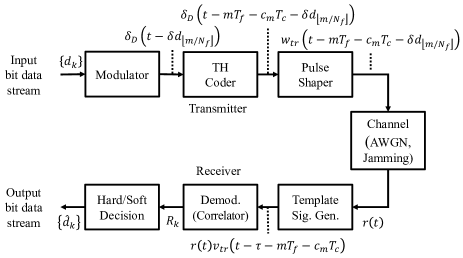
Figure 1: Block diagram of TH systems.

A block diagram of TH systems is shown graphically in Fig. 1. In this figure, $\delta_{D}(t)$ is the Dirac delta function [22] and $\left\{d_{k}\right\}$ denotes a stream of data bits, in which each bit is of duration $T_{b}$ composed of $N_{f}=T_{b}/T_{f}$ frames of duration $T_{f}$. A frame in turn consists of $N_{c}=T_{f}/T_{c}$ chips of duration $T_{c}$, where $T_{c}\ll T_{f}$ in practice. The transmitted waveform $w_{tr}(t)$ of the TH system, in the form of pulses with a very short duration, is often called a monocycle. The duration $T_{p}$ of a monocycle is usually chosen to be $T_{p}<T_{c}$ and is in the order of $1$ ns yielding a bandwidth in the order of $1$ GHz.

For the transmission of the data stream $\left\{d_{k}\right\}$, we first generate a TH code $\left\{c_{m}\right\}_{m=1}^{N_{h}}$, a set of independent and identically distributed random variables over $\left\{1,2,...,N_{c}\right\}$. The TH code determines the location of a chip within a frame: For example, when $c_{5}=3$, we transmit a monocycle at the third chip in the fifth frame. When the TH-PPM is employed, a monocycle is delayed by the PPM shift $\delta$ and $0$ for a data bit ‘1’ and ‘0’, respectively. The transmitted waveform of the TH-PPM can then be written as [2]

$$s_{PPM}(t)=\sum_{m=-\infty}^{\infty}w_{tr}\left(t-mT_{f}-c_{m}T_{c}-\delta d_{\lfloor m/N_{f}\rfloor}\right),$$ (1)

where $\lfloor\cdot\rfloor$ is the floor function. The signal $r(t)$ received at the receiver can subsequently be written as

$$r(t)=\alpha s_{PPM}(t-\tau)+j(t)+n(t),$$ (2)

where $\alpha$ is the channel gain, $\tau$ is a random variable over $\left[0,\infty\right)$ representing the time asynchronism between the transmitter and receiver, $j(t)$ is the jamming signal, and $n(t)$ is the AWGN.

When a correlator receiver is employed, the received signal $r(t)$ is correlated with the template signal

$$v_{tr}(t)=w_{tr}(t)-w_{tr}(t-\delta)$$ (3)

of the monocycle $w_{tr}(t)$. Assuming a perfect synchronization (i.e., $\tau$, $c_{m}$, $T_{f}$, and $T_{c}$ are available at the receiver), the output of the correlator for the $k$-th bit can be expressed as

$$R_{k} = \sum_{m=kN_{f}}^{(k+1)N_{f}-1}\int_{\tau+mT_{f}}^{\tau+(m+1)T_{f}}r(t)$$ (4)

$$\quad\times v_{tr}\left(t-\tau-mT_{f}-c_{m}T_{c}\right)dt$$

$$= S_{k}+J_{k}+N_{k},$$

where $S_{k},J_{k}$, and $N_{k}$ are the correlator outputs corresponding to the TH signal $s_{PPM}(t)$, jamming signal $j(t)$, and AWGN $n(t)$, respectively. The decision hypothesis that a data bit of ‘0’ is sent is chosen if $R_{k}\geq 0$: Specifically,

$$\widehat{d}_{k}=\frac{1}{2}\left\{1-\mbox{sgn}\left(R_{k}\right)\right\}$$ (5)

is the estimate of $d_{k}$.

II-B Tone Jamming Models

When a jamming signal has a single and a multitude of frequencies, it is called an STJ and a MTJ signals, respectively [10]. In this paper, we assume the STJ model, which can be a serious attack with a concentrated power. The jamming signal $j(t)$ in (2) can be expressed more specifically as

$$j_{STJ}\left(t;f_{J},\theta_{J}\right)=\sqrt{2P_{J}}\cos\left(2\pi f_{J}t+\theta_{J}\right),$$ (6)

where $P_{J}$, $f_{J}$, and $\theta_{J}$ are the power, frequency, and phase, respectively, of the STJ signal.

II-C Correlation between TH and Jamming Signals

Let us denote the correlation function between the jamming and template signals by

$$R_{tr,T}\left(z;\theta_{J},f_{J},T_{c}\right)$$ (7)

$$=\int_{0}^{T_{c}}{v_{tr}(t)\cos(2\pi f_{J}\left(t+z)+\theta_{J}\right)dt}$$

using (6) for an STJ, where the constant $\sqrt{2P_{J}}$ is omitted for simplicity.

Since the template signal $v_{tr}\left(t-\tau-mT_{f}-c_{m}T_{c}\right)$ has non-zero values only during one chip duration of $T_{c}$, i.e.,

$$mT_{f}+c_{m}T_{c}\leq t-\tau\leq mT_{f}+(c_{m}+1)T_{c}$$ (8)

per one frame, the correlator output $J_{k}$ in (4) of the jamming signal for the $k$-th bit can be expressed in general as

$$J_{k} = \sum_{m=kN_{f}}^{(k+1)N_{f}-1}\int_{\tau+mT_{f}}^{\tau+(m+1)T_{f}}j(t)v_{tr}\left(t-\tau-mT_{f}-c_{m}T_{c}\right)dt$$ (9)

$$= \sum_{m=kN_{f}}^{(k+1)N_{f}-1}\int_{\tau+mT_{f}+c_{m}T_{c}}^{\tau+mT_{f}+\left(c_{m}+1\right)T_{c}}j(t)$$

$$\quad\qquad\qquad\times v_{tr}\left(t-\tau-mT_{f}-c_{m}T_{c}\right)dt$$

$$= \sum_{m=kN_{f}}^{(k+1)N_{f}-1}{R_{tr,T}\left(\Delta_{m};\theta_{J},f_{J},T_{c}\right)},$$

where

$$\Delta_{m}=\tau+mT_{f}+c_{m}T_{c}$$ (10)

denotes the time shift between the template signal $v_{tr}\left(t-\tau-mT_{f}-c_{m}T_{c}\right)$ of the TH system and jamming signal $j(t)$ at the $m$-th frame. It is noteworthy that possible values of the time shift $\Delta_{m}$ in (9) under the influence of the STJ signal (6) are

$$\mathrm{mod}\left(\mathrm{mod}\left(nT_{J}-\tau,T_{c}\right),T_{J}\right),$$ (11)

where $n$ is an integer and $T_{J}=1/f_{J}$ is the period of the jamming signal. Since $\tau$ is a random variable and $T_{c}$ is not an integer multiple of $T_{J}$ in general, $\Delta_{m}$ is also a random variable.

II-D Clipper

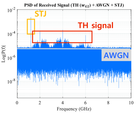
Figure 2: PSD of the received signal with the components of TH signal, STJ signal, and noise specified.

Fig. 2 shows an example of the power spectral density (PSD) $P_{rec}(f)$ of the received signal $r(t)$ under the STJ model in terms of the TH, STJ, and AWGN components when the Gaussian doublet

$$w_{G2}\left(t+T_{m}\right)=A\left\{1-4\pi\left(\frac{2t}{T_{p}}\right)^{2}\right\}\exp\left\{-2\pi\left(\frac{2t}{T_{p}}\right)^{2}\right\},$$ (12)

one of the waveforms employed most commonly in TH systems, is used as the monocycle, where $A$ is the amplitude and $T_{m}$ denotes the center of the waveform.

The clipper [23], a simple AJ filter with a threshold, limits the signal based on the second largest value of $\left|P_{rec}(f)\right|$: Normally, an STJ signal exhibits the maximum peak of the PSD due to its concentration at a frequency, and the second largest value is $\max|P_{TH}(f)|$, where $P_{TH}(f)$ is the PSD of the TH signal. Therefore, the clipping threshold $\lambda_{C}$ is determined as

$$\lambda_{C}=K\max|P_{TH}(f)|,$$ (13)

where the constant $K$ is often selected in the interval $[1,1.5]$: In this paper, we choose $K=1.2$, and assume a clipper at the receiver for all the waveforms later in the comparisons and further investigation of the AJ performance of the waveform from the proposed design.

III Design of Waveforms

III-A Problem Formulation

We now consider the design of waveforms to enhance the AJ capability of the TH system against the STJ. The correlation function $R_{tr,T}$ in (9) is a sinusoidal function of $\Delta_{m}$. Since the maximum value of the correlator output with respect to $\Delta_{m}$ determines the AJ performance, the cost function is

$$\max_{\Delta_{m}}\left|R_{tr,T}\left(\Delta_{m};\theta_{J},f_{J},T_{c}\right)\right|.$$ (14)

Let us try to find the optimal waveform $\widehat{w}_{tr}(t)$ that minimizes the cost function under the constraint $\left\|\widehat{w}_{tr}(t)\right\|^{2}=1$. We assume that $T_{c}$ is given and $\theta_{J}$ is equal to zero, and thus the term $\theta_{J}$ will not be shown explicitly from now on. Then, denoting by $\widehat{f}_{J}$ the estimate of the actual jammer frequency $f_{J}$, the problem of waveform design can be formulated as

$$\widehat{w}_{tr,\widehat{f}_{J}}(t)= \arg\min_{w_{tr}}\max_{\Delta_{m}}\left|R_{tr,T}\left(\Delta_{m};\widehat{f}_{J},T_{c}\right)\right|$$ (15)

$$\mbox{such that }\left\|\widehat{w}_{tr}(t)\right\|^{2}=1.$$

III-B Problem Simplification

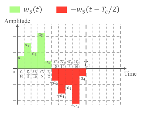
Figure 3: Approximation of waveform $w_{tr}(t)$ as a weighted sum of $N=5$ rectangular pulses

The problem (15) is rather intractable mainly due to the minimization and maximization over continuous spaces involved in the optimization. To make the problem somewhat tractable, we consider an approximation

$$w_{N}(t)=\sum_{i=1}^{N}{a_{i}\mbox{rect}\left(\frac{t-(2i-1)\tfrac{T_{c}}{4N}}{\tfrac{T_{c}}{2N}}\right)}$$ (16)

of the TH waveform $\widehat{w}_{tr,\widehat{f}_{J}}(t)$, where $\left\{a_{i}\right\}_{i=1}^{N}$ are the weights for the $N$ rectangular pulses $\mbox{rect}(\cdot)$ of duration ${T_{p}}/{N}$ with $T_{p}=T_{c}/2$ as shown in Fig. 3. Then, with the template signal

$$v_{N}(t)=w_{N}(t)-w_{N}\left(t-\frac{T_{c}}{2}\right),$$ (17)

the correlation $R_{tr,T}$ in (9) can be expressed as

$$R_{N,T}\left(\Delta_{m};f_{J},T_{c}\right)$$ (18)

$$\quad=A_{N}\left(f_{J};T_{c}\right)B_{N}\left(\Delta_{m},f_{J},\left\{a_{i}\right\};T_{c}\right)$$

by substituting (16) and $\theta_{J}=0$ in (7), where

$$A_{N}\left(f;t\right)=\frac{2}{\pi f}\sin\frac{\pi ft}{2}\sin\frac{\pi ft}{2N}$$ (19)

and

$$B_{N}\left(\alpha,f,\left\{a_{i}\right\};t\right)=\sum_{i=1}^{N}{a_{i}\sin\left\{\pi f\left(\frac{N-1+2i}{2N}t+2\alpha\right)\right\}}.$$ (20)

By noting that $A_{N}\left(f_{J};T_{c}\right)$ is independent of $\Delta_{m}$, that $B_{N}\left(\Delta_{m},f_{J},\left\{a_{i}\right\};T_{c}\right)$ is a sum of sinusoids at the same frequency, and that the sum of sinusoids of the same frequency with possibly different phases and amplitudes is also a sinusoid at that frequency, we have

$$F_{N}\left(f_{J},\left\{a_{i}\right\};T_{c}\right) = \left|A_{N}\left(f_{J};T_{c}\right)\right|$$ (21)

$$\quad\times\max_{\Delta_{m}}\left|B_{N}\left(\Delta_{m},f_{J},\left\{a_{i}\right\};T_{c}\right)\right|$$

$$= \left|A_{N}\left(f_{J};T_{c}\right)\right|\sqrt{\mathcal{X}_{N}^{2}+\mathcal{Y}_{N}^{2}}$$

from (18)-(20), where

$$F_{N}\left(f,\left\{a_{i}\right\};t\right)=\max_{\alpha}\left|R_{N,T}\left(\alpha;f,t\right)\right|,$$ (22)

$$\mathcal{X}_{N}=\sum_{i=1}^{N}{a_{i}\cos\frac{N-1+2i}{2N}\pi f_{J}T_{c}},$$ (23)

and

$$\mathcal{Y}_{N}=\sum_{i=1}^{N}{a_{i}\sin\frac{N-1+2i}{2N}\pi f_{J}T_{c}}.$$ (24)

Employing (21) in (15), we can express the problem of designing waveforms with the estimated frequency $\widehat{f}_{J}$ as

$$\widehat{W}_{N,\widehat{f}_{J}}= \arg\min_{\left\{a_{i}\right\}_{i=1}^{N}}{F_{N}\left(\widehat{f}_{J},\left\{a_{i}\right\};T_{c}\right)}$$ (25)

$$\mbox{such that }\sum_{i=1}^{N}{a_{i}^{2}}=1,$$

where

$$\widehat{W}_{N,\widehat{f}_{J}}=\left\{\hat{a}_{k}\right\}_{k=1}^{N}$$ (26)

denotes a set of $N$ coefficients of $\widehat{w}_{N,\widehat{f}_{J}}(t)$, an approximation of the optimal waveform $\widehat{w}_{tr,\widehat{f}_{J}}(t)$ defined in (15) with $N$ rectangular pulses.

Let us in passing note that

$$A_{N}\left(f;T_{c}\right)=0$$ (27)

if $fT_{c}=2kN$ for an integer $k$. In addition, $A_{N}\left(f;T_{c}\right)$ decreases rather fast as $f$ increases beyond $f=\frac{2N}{T_{c}}$. Therefore, we will concentrate on the range from $0$ to $\frac{2N}{T_{c}}$ Hz of jamming frequency.

III-C Solutions and Algorithms

Let us note that the maximum $F_{N}$ in (25) can now be rewritten as

$$F_{N}\left(\widehat{f}_{J},\left\{a_{i}\right\};T_{c}\right)=\left|A_{N}\left(\widehat{f}_{J};T_{c}\right)\right|$$ (28)

$$\times\sqrt{\sum_{i=1}^{N}{a_{i}^{2}}+2\sum_{n=1}^{N-1}\cos{\frac{\pi n\widehat{f}_{J}T_{c}}{N}}{\sum_{k=1}^{N-n}{a_{k}a_{k+n}}}}$$

$$=\left|A_{N}\left(\widehat{f}_{J};T_{c}\right)\right|\sqrt{\mathbf{a}^{T}\,\mathcal{C}\mathbf{a}}$$

from (21), where $\mathbf{a}=\left[a_{1},a_{2},...,a_{N}\right]^{T}$ and the matrix $\mathcal{C}$ has

$$c_{i,j}=\cos\left(\frac{\pi\widehat{f}_{J}T_{c}\left|i-j\right|}{N}\right)$$ (29)

as its $(i,j)$-th elements. The problem (25) of designing waveforms with (28) can thus be represented as a minimization of $\mathbf{a}^{T}\,\mathcal{C}\mathbf{a}$, for which the solution should satisfy the Karush–-Kuhn–-Tucker (KKT) conditions [24]

$$\mathbf{a}^{T}\left(\mathcal{C}-\lambda I\right)=0;\qquad\mathbf{a}^{T}\mathbf{a}=1;\qquad\lambda>0.$$ (30)

The KKT conditions (30) imply that the solution to the minimization of $\mathbf{a}^{T}\,\mathcal{C}\mathbf{a}$ will be the normalized eigenvectors of the positive eigenvalues of the matrix $\mathcal{C}$. The waveform solution to (25) for mitigating the STJ can thus be obtained, for example, by Powell’s conjugate‐-direction method [25] after taking the conditions (30) into account as described in Algorithm 1, where $\left[\mathbf{u}_{1},\mathbf{u}_{2},...,\mathbf{u}_{N}\right]$ denotes a set of initial direction vectors and $\mathbf{e}_{i}$ is the standard unit vector.

Data: An estimate $\widehat{f}_{J}$ of $f_{J}$, $h(\mathbf{a})=\mathbf{a}^{T}\,\mathcal{C}\mathbf{a}$,

        Initial $\mathbf{a}_{i}$

Result: $\hat{\mathbf{a}}\leftarrow\mathbf{a}_{i}$

1 while $\mathcal{C}\mathbf{a}_{i}\neq\lambda\mathbf{a}_{i}$ for some $\lambda>0$ do

2       $\left[\mathbf{u}_{1},\mathbf{u}_{2},...,\mathbf{u}_{N}\right]\leftarrow\left[\mathbf{e}_{1},\mathbf{e}_{2},...,\mathbf{e}_{N}\right]$.

3       $i\leftarrow 1$.

4       Initialize $\mathbf{a}_{i}$.

5       while not converged do

6             $\mathbf{p}_{0}\leftarrow\mathbf{a}_{i}$

7             for $k=1,2...N$ do

8                  $\hat{\gamma}_{k}\leftarrow\arg\min_{\gamma_{k}}{h\left(\mathbf{p}_{k-1}+\gamma_{k}\mathbf{u}_{k}\right)}$.

9                   $\mathbf{p}_{k}\leftarrow\mathbf{p}_{k-1}+\hat{\gamma}_{k}\mathbf{u}_{k}$.

10             end for

11            $i\leftarrow i+1$.

12             for $j=1,2,...,N-1$ do

13                  $\mathbf{u}_{j}\leftarrow\mathbf{u}_{j+1}$.

14             end for

15            $\mathbf{u}_{N}\leftarrow\mathbf{p}_{N}-\mathbf{p}_{0}$.

16             $\hat{\gamma}\leftarrow\arg\min_{\gamma}{h\left(\mathbf{p}_{0}+\gamma\mathbf{u}_{N}\right)}$.

17             $\mathbf{a}_{i}\leftarrow\mathbf{p}_{0}+\hat{\gamma}\mathbf{u}_{N}$.

18       end while

19      

20 end while

Algorithm 1 Design of AJ waveforms against STJ with Powell’s method

III-D Challenges and Possible Solutions in Other Jamming Scenarios

The proposed design of waveforms provides us with an optimality against STJ; yet, we will probably encounter in practice with other more complex and intelligent jamming scenarios. Let us briefly describe how we can generalize and extend the proposed waveform design for coping with the challenges in such various jamming scenarios.

Many intelligent jamming (IJ), such as the MTJ, TV-STJ, and SWJ as mentioned before, schemes are based on the concepts of optimization, awareness, game theory, and software defined communications for the efficiency and effectiveness of jammers. With the knowledge of the protocol, IJ schemes are shown to perform (from the viewpoint of jammers) better than the trivial continuous high power noise jamming while also retaining its effectiveness: More specifically, IJ schemes are reported to be more efficient than the periodic and trivial jammings by one to two and five, respectively, orders of magnitude [26].

Now, although application of the proposed waveforms against STJ directly to the MTJ cases may not be promising, the design of waveforms against MTJ can be formulated, for example, as

$$\widehat{w}_{tr,\widehat{\mathcal{F}}_{J}}(t)= \arg\min_{w_{tr}}\max_{\Delta_{m}}\sum_{\omega=1}^{\Omega}\left|R_{tr,T}\left(\Delta_{m};\widehat{f}_{J,\omega},T_{c}\right)\right|$$ (31)

$$\mbox{such that }\left\|\widehat{w}_{tr}(t)\right\|^{2}=1$$

by extending (15) to take the multiple estimates

$$\widehat{\mathcal{F}}_{J}=\left\{\widehat{f}_{J,\omega}\right\}_{\omega=1}^{\Omega}$$ (32)

of jamming frequencies into consideration. We expect that simplification and/or approximation of the problem (31) for the design of waveforms against MTJ would provide us with some insight or solution for possible practical implementation. We would also like to note that MTJ with the jamming frequencies falling inside (a small portion of) the bandwidth of the TH SS systems can statistically be considered as a STJ in the perspective of the AJ performance [4].

The TV-STJ is a subclass of random jamming, in which several tones varying in time are employed [16]. The waveforms designed by the proposed technique can clearly be employed within periods the TV-STJ. When the variation of the TV-STJ is very fast, the problem could possibly be modeled and solved with the methods of signal detection and classification, widely developed by utilizing energy detectors, higher-order statistical features, and statistical tests [27]: They can also be achieved by using learning methods based on techniques of neural networks as shown in [28, 29].

For SWJ, which swepdf a narrow-band jamming signal over a wide frequency band, sinusoidal signals are widely used with a linear sweep method because of simplicity and usefulness [8]. By viewing the SWJ as a TV-STJ, the technique described above against the TV-STJ can similarly be applied against SWJ by optimizing waveforms periodically. Alternatively, by generalizing (15) again, we can design a waveform against the SWJ over the bandwidth of the SWJ as

$$\widehat{w}_{tr,\widehat{\mathcal{F}}_{J}}= \arg\min_{w_{tr}}\max_{\Delta_{m}}\int_{\widehat{f}_{J,l}}^{\widehat{f}_{J,u}}\left|R_{tr,T}\left(\Delta_{m};f,T_{c}\right)\right|df$$ (33)

$$\mbox{such that }\left\|\widehat{w}_{tr}(t)\right\|^{2}=1,$$

for example, where $\widehat{\mathcal{F}}_{J}=\left\{\widehat{f}_{J,l},\widehat{f}_{J,u}\right\}$ now denotes the set of estimates of the lower and upper jamming frequencies of the SWJ. The problem (33) is applicable to the partial-band noise jamming signal as well, but is rather intractable for a direct solution mainly due to the minimization, maximization, and integration over continuous spaces involved in the optimization. Apparently, simplification and/or approximation of the problem (33) would constitute a good topic for a future study.

IV Numerical and Simulation Results

In this section, we discuss the performance of the proposed method of designing waveforms via numerical and simulation results for $N=5$ and $T_{c}=1$ ns with the pulse duration $T_{p}=T_{c}/2=0.5$ ns and approximate bandwidth of $5$ GHz as in [12]. Normally, TH SS systems are deployed in network applications; yet, to focused fully on the effects of jammer [4], we consider scenarios with one-node-only and static setup without taking mobility, Doppler’s effect, and inter-node interference into consideration.

IV-A Numerical Results

From (19)-(24), we have

$$F_{5}(f_{J},\left\{a_{i}\right\};1)=\left|A_{5}(f_{J};1)\right|\sqrt{\mathcal{X}_{5}^{2}+\mathcal{Y}_{5}^{2}},$$ (34)

where

$$A_{5}(f;1)=\frac{2}{\pi f}\sin\frac{\pi f}{2}\sin\frac{\pi f}{10},$$ (35)

$$\mathcal{X}_{5}=\sum_{i=1}^{5}{a_{i}\cos\frac{i+2}{5}\pi f_{J}},$$ (36)

$$\mathcal{Y}_{5}=\sum_{i=1}^{5}{a_{i}\sin\frac{i+2}{5}\pi f_{J}},$$ (37)

and $f_{J}$ is in GHz.

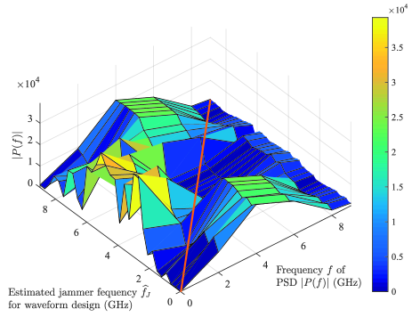
Figure 4: Spectrogram of the optimal waveforms. Each row represents the PSD of the waveform optimized for the estimated jammer frequency $\widehat{f}_{J}$.

Fig. 4 shows the spectrogram of the waveform optimized for the estimated jammer frequency $\widehat{f}_{J}$, where the color density represents the PSD of the waveform. It is clearly observed that the lowest PSD is located at the frequency for which the waveform is optimized: i.e., colors on the diagonal line are generally darker blue (meaning lower PSD values) than those away from the diagonal line.

Let us next consider the BER performance of some waveforms with simulation parameters $N_{f}=3$, $N_{c}=4$, $N_{p}=100$, $T_{f}=4$ ns, $T_{m}=0.25$ ns, $T_{p}=0.5$ ns, $\delta=0.5$ ns, and a sampling interval of 0.02 ns for all signals [4]: We have chosen $T_{f}=4$ for simplicity in the simulations although it does not completely satisfy the condition $T_{f}\gg T_{c}$ of practical cases.

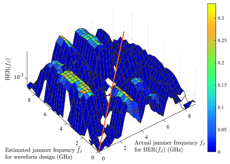
Figure 5: BER performance of the optimal waveform at $f_{J}$ versus $f$.

Fig. 5 simulates the BER performance of the TH system with the waveforms optimized for the estimated jammer frequency $\widehat{f}_{J}$ versus the actual jammer frequency $f_{J}$. The BER performance along the diagonal line is very close to the minimum simulated BER of $2.5\times 10^{-7}$: This implies that the proposed design of waveforms improves the BER performance of the TH system when the estimate $\widehat{f}_{J}$ is close to $f_{J}$. As the BER is observed to decrease sharply over 8 GHz, we will mainly focus on the interval $[0,9]$ GHz from now on.

In the following simulations, we mainly show the results for the actual jamming frequency $f_{J}$ of $1.5$, $3.0$, and $6.6$ GHz for a clarity reason in the figures: Let us mention that we have nonetheless performed simulations from 0 to 9 GHz in an interval of 0.3 GHz. The AJ performance of the TH systems with the optimized waveforms $\widehat{w}_{5,1.5}(t)$, $\widehat{w}_{5,3.0}(t)$, and $\widehat{w}_{5,6.6}(t)$ are compared with that of the TH system with the conventional waveform and that of the TH system with the clipper receiver described by the threshold (13). Here, the ‘conventional’ waveform we considered is the Gaussian doublet

$$w_{G2}(t+0.25)=A\left(1-64\pi t^{2}\right)\exp\left(-32\pi t^{2}\right)$$ (38)

with the unit of $t$ in ns [2], and the optimized waveforms $\widehat{w}_{5,1.5}(t)$, $\widehat{w}_{5,3.0}(t)$, and $\widehat{w}_{5,6.6}(t)$ can be expressed by

$$\widehat{W}_{5,\textrm{1.5}}=\left\{-0.441,\,0.717,\,-0.517,0.013,\,0.157\right\},$$ (39)

$$\widehat{W}_{5,\textrm{3.0}}=\left\{0.487,\,0.523,\,0.656,\,0.241,\,0.032\right\},$$ (40)

and

$$\widehat{W}_{5,\textrm{6.6}}=\left\{-0.282,\,0.662,\,0.197,\,0.370,\,-0.554\right\},$$ (41)

respectively, as obtained by solving (25) numerically with Algorithm 1. The waveforms $w_{G2}(t)$, $\widehat{w}_{5,\textrm{1.5}}(t)$, $\widehat{w}_{5,\textrm{3.0}}(t)$, and $\widehat{w}_{5,\textrm{6.6}}(t)$ are shown in Fig. 6 with STJ signals at 1.5, 3.0, and 6.6 GHz.

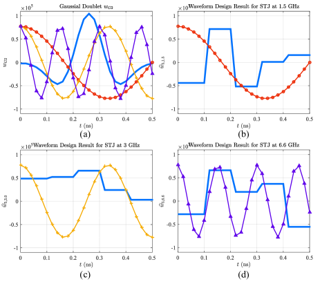
Figure 6: Proposed waveforms of the TH system (the blue curve) with $N=5$ against STJ signals of SJR=$0$ dB at 1.5 (the red curve with ‘O’ markers), 3.0 (the yellow curve with ‘+’ markers), and 6.6 GHz (the purple curve with ‘$\triangle$’ markers): (a) $w_{G2}$, (b) $\widehat{w}_{5,\textrm{1.5}}$, (c) $\widehat{w}_{5,\textrm{3.0}}$, and (d) $\widehat{w}_{5,\textrm{6.6}}$.

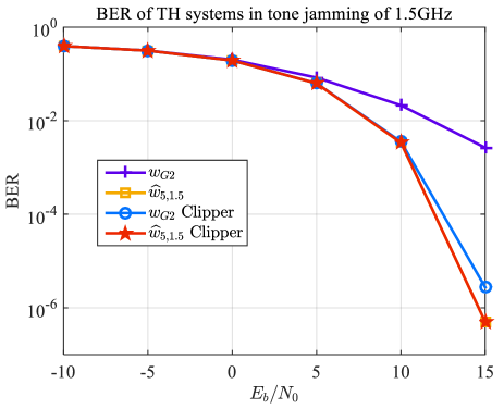
Figure 7: Comparison of BER of the TH systems with $\widehat{w}_{5,\textrm{1.5}}$ (the yellow curve with ‘$\Box$’ markers), with $\widehat{w}_{5,\textrm{1.5}}$ and the clipper (the red curve with ‘$\medstar$’ markers), with $w_{G2}$ (the purple curve with ‘+’ markers), and with $w_{G2}$ and the clipper (the blue curve with ‘O’ markers) in an AWGN channel with STJ of SJR=$-10$ dB at 1.5 GHz.

In Fig. 7, we compare the BER of the TH systems employing $\widehat{w}_{5,\textrm{1.5}}$ (the yellow curve with ‘$\Box$’ markers), $\widehat{w}_{5,\textrm{1.5}}$ with clipping (the red curve with ‘$\medstar$’ markers), $w_{G2}$ (the purple curve with ‘+’ markers), and $w_{G2}$ with clipping (the blue curve with ‘O’ markers) over an AWGN channel with signal-to-jamming ratio (SJR) of $-10$ dB and $f_{J}=1.5$ GHz. The BER of the TH system with the optimized waveform $\widehat{w}_{5,\textrm{1.5}}$ is clearly lower than that with the conventional Gaussian doublet $w_{G2}$ even with clipping.

Additionally, $\widehat{w}_{5,\textrm{1.5}}$ exhibits the same BER performance regardless of the clipper at the receiver. This implies that the clipper does not provide an additional improvement of performance beyond the optimization of waveform design. We have confirmed that the same observation holds when the jammer frequency is of other values between 0 and 9 GHz although not specifically shown in this figure for brevity. In order to investigate the advantages of the proposed design technique of waveforms conservatively, we assume the clipper receiver is embedded in TH systems from now on.

IV-B Simulation Results

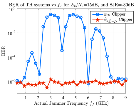
Figure 8: BER performance versus jammer frequency $f_{J}$ of the TH systems employing the optimized waveform $\widehat{w}_{5,\widehat{f}_{J}=f_{J}}$ (the red curve with ‘$\medstar$’ markers) and Gaussian doublet $w_{G2}$ (the blue curve with ‘O’ markers) over an AWGN channel of $E_{b}/N_{0}=15$ dB and SJR=$-30$ dB.

Fig. 8 presents the BER performance versus the actual jammer frequency $f_{J}$ of the TH systems employing the optimized waveform $\widehat{w}_{5,\widehat{f}_{J}=f_{J}}$ (the red curve with ‘$\medstar$’ markers) and Gaussian doublet $w_{G2}$ (the blue curve with ‘O’ markers) over an AWGN channel with the bit energy to noise power spectral density ($E_{b}/N_{0}$) $15$ dB and SJR=$-30$ dB. At almost all values from 0 to 9 GHz of the jammer frequency, the simulation results again show that the optimized waveforms generally outperform the conventional scheme with clipping. The improvement of AJ performance with the optimized waveforms over the Gaussian doublet becomes very large when the jammer frequency is 3, 5, and 6.5 GHz, at which the Gaussian doublet has most of its power.

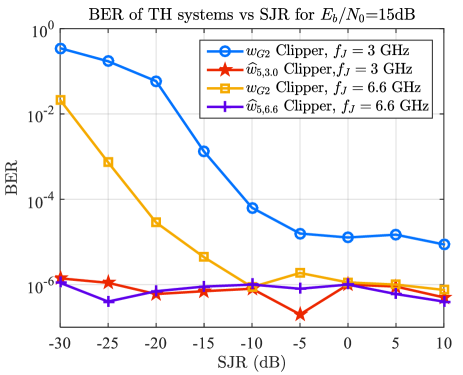
Figure 9: BER performance of the TH systems with the optimized waveform $\widehat{w}_{5,3.0}$ (the red curve with ‘$\medstar$’ markers) and Gaussian doublet $w_{G2}$ (the blue curve with ‘O’ markers) against an STJ at 3 GHz, and the optimized waveform $\widehat{w}_{5,6.6}$ (the purple curve with ‘+’ markers) and Gaussian doublet $w_{G2}$ (the yellow curve with ‘$\Box$’ markers) against an STJ at 6.6 GHz.

In Fig. 9, we consider the BER performance of the TH systems with the optimized waveform $\widehat{w}_{5,3.0}$ (the red curve with ‘$\medstar$’ markers) and with the Gaussian doublet $w_{G2}$ (the blue curve with ‘O’ markers) for the STJ at $f_{J}=3$ GHz when $E_{b}/N_{0}=15$ dB. The BER of the TH systems with $w_{G2}$ (the yellow curve with ‘$\Box$’ markers) and with $\widehat{w}_{5,6.6}$ (the purple curve with ‘+’ markers) for the STJ at $f_{J}=6.6$ GHz are also shown. We observe that the optimized waveforms $\widehat{w}_{5,3.0}$ and $\widehat{w}_{5,6.6}$ provide a stable AJ performance of BER=$10^{-6}$ even when the SJR of the STJ varies. On the other hand, the BER of the TH system with $w_{G2}$ becomes worse as the SJR decreases. In addition, when the SJR increases, the BER performance of $w_{G2}$ for $f_{J}=3.3$ GHz is saturated at the level of $10^{-5}$, a value (roughly 10 times) higher than that of the proposed waveform. We have confirmed that the same observation holds at other values in the range $[0,9]$ GHz of the jammer frequency.

IV-C Imperfect Estimation of Jamming Frequency

We have so far assumed idealistically perfect estimation of $f_{J}$, which is not always possible in practical scenarios especially when the jammer power is not strong enough. Let us now consider the scenario that an estimation error

$$\varepsilon_{f}=\widehat{f}_{J}-f_{J}$$ (42)

occurs in estimating the jammer frequency $f_{J}$. The estimation error $\varepsilon_{f}$ is commonly assumed to follow a Gaussian distribution, i.e.,

$$\varepsilon_{f}\sim\mathcal{N}\left(\mu_{\varepsilon_{f}},\sigma_{\varepsilon_{f}}^{2}\right),$$ (43)

where $\mu_{\varepsilon_{f}}$ and $\sigma_{\varepsilon_{f}}$ are the mean and standard deviation of $\varepsilon_{f}$, respectively [30].

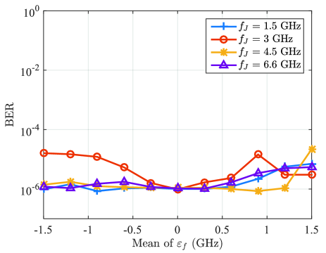
Figure 10: BER performance of the TH systems employing $\widehat{w}_{5,\widehat{f}_{J}}$ versus the mean of the estimation error $\varepsilon_{f}=\widehat{f}_{J}-f_{J}$ when the standard deviation of the estimation error is 0 over an AWGN channel of $E_{b}/N_{0}=15$ dB and STJ of SJR=$-10$ dB at 1.5 (the blue curve with ‘+’ marker), 3 (the red curve with ‘O’ markers), 4.5 (the yellow curve with ‘*’ markers), and 6.6 GHz (the purple curve with ‘$\bigtriangledown$’ markers).

Fig. 10 shows the BER performance of the TH system with $\widehat{w}_{5,\widehat{f}_{J}}$ versus $\mu_{\varepsilon_{f}}$ when $\sigma_{\varepsilon_{f}}=0$ for several values of STJ frequency. The simulation results in this figure indicate that the proposed design of waveforms provides a reasonable BER level of $2\times 10^{-5}$ even when the mean of the estimation error is from -1.5 to 1.5 GHz. When $\mu_{\varepsilon_{f}}=-1.5$ and $0.9$ GHz, the AJ performance of the TH system with the proposed design of waveforms degrades mostly under the STJ with $f_{J}=3$ GHz: Yet, even this most severe degradation provides a BER of $10^{-5}$ approximately, a value much better than the BER $8\times 10^{-5}$ with $w_{G2}$ (shown in Fig. 9). In the cases of 1.5 and 6.6 GHz of $f_{J}$, the estimation error from -1.5 to 0.3 GHz does not influence the AJ performance of the TH systems with the proposed design of waveforms significantly. The proposed design of waveforms also exhibits a robustness property against estimation errors from $-1.5$ to $1.2$ GHz for an STJ of $f_{J}=4.5$ GHz.

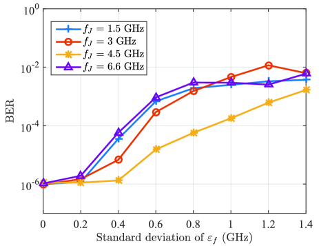
Figure 11: BER performances of the TH systems employing $\widehat{w}_{5,\widehat{f}_{J}}$ versus the standard deviation of the estimation error $\varepsilon_{f}=\widehat{f}_{J}-f_{J}$ over an AWGN channel of $E_{b}/N_{0}=15$ dB and STJ of SJR=$-10$ dB at 1.5 (the blue curve with ‘+’ marker), 3 (the red curve with ‘O’ markers), 4.5 (the yellow curve with ‘*’ markers), and 6.6 GHz (the purple curve with ‘$\bigtriangledown$’ markers).

Fig. 11 presents the BER performance of the TH system with $\widehat{w}_{5,\widehat{f}_{J}}$ versus $\sigma_{\varepsilon_{f}}$ when $\mu_{\varepsilon_{f}}=0$ under STJ with various values of jamming frequency. It is observed that $\sigma_{\varepsilon_{f}}$ of the estimator should be less than 0.46, 0.54, 0.9, and 0.43 GHz when $f_{J}=1.5,3,4.5,$ and $6.6$ GHz, respectively, to ensure a BER level of $10^{-4}$. The proposed design of waveforms clearly provides a BER performance of $10^{-5}$ when the standard deviation of the estimation error is less than 0.3 GHz for almost all values from 0 to 9 GHz of jammer frequency although we have shown the results only for $f_{J}=1.5,3,4.5,$ and $6.6$ GHz for a brevity reason in this figure. In addition, we have considered the influence of the mean and variance of the estimation error only for limited cases: Yet, we believe that the standard deviation $\sigma_{\varepsilon_{f}}$ of the estimation error is more crucial than the mean $\mu_{\varepsilon_{f}}$ of the estimation error when estimating the jammer frequency $f_{J}$ in the design of AJ waveforms.

V Conclusion

In this paper, the problem of designing waveforms with an aim of improving the anti-jamming performance against STJ has been addressed. The problem of designing waveform is formulated and simplified by analyzing the correlation between the TH and jamming signals. Assuming an estimate of the frequency of STJ signal is available, an algorithm is provided for the design of suboptimal waveforms.

The waveforms designed with a perfect estimate of the jamming frequency outperform the conventional Gaussian doublet regardless of the clipper for almost all values from 0 to 9 GHz of jammer frequency. We have in addition observed that the proposed design can provide us with waveforms that overcome the unavoidable saturation of the BER performance of the conventional Gaussian waveform even with a clipper.

In the case of non-ideal estimation of the jamming frequency, simulation results showed that the AJ capability the waveforms designed with the proposed scheme still maintain a reasonable BER level of $2\times 10^{-5}$ even when the mean of estimation error is in the range of $[-1.5,1.5]$ GHz. In addition, the proposed design of waveforms can provide a BER performance of $10^{-5}$ when the standard deviation of the estimate is less than 0.3 GHz for almost all values from 0 to 9 GHz of jammer frequency. We have also observed that the standard deviation of the estimation error from the estimation of jammer frequency is more influential than the mean of the estimation error in the design of AJ waveforms. Finally, the proposed design of waveforms exhibits robustness to the estimation errors of the jammer frequency.

We wish to add that consideration of complex and intelligent jamming scenarios (including the MTJ, TV-STJ, and SWJ) in the design of waveforms, and investigation of joint optimization of power allocation schemes and waveform design are expected to be highly promising and fruitful topics for further studies.

Hyoyoung Jung (S’12) received the B.S. degree in electronic engineering from Inha University, South Korea, in 2011. He is currently pursuing the M.S. and Ph.D. integrated degree in electrical engineering and computer science from the Gwangju Institute of Science and Technology, South Korea. His research interests include statistical signal processing, machine learning, and anti-jamming communication systems.

Binh Van Nguyen received the bachelor degree in electrical and electronics from the Ho Chi Minh City University of Technology, Ho Chi Minh City, Vietnam, in 2010, and the M.S. and the Ph.D. degree in wireless communications from the Gwangju Institute of Science and Technology (GIST), Gwangju, Republic of Korea, in 2012 and 2016, respectively. From Sep. 2016 to Oct. 2018, he worked as a Research Fellow at GIST. From Nov. 2018 to Aug. 2019, he worked as an Assistant Research Professor at GIST. He is now with Samsung Electronics, Suwon, Republic of Korea, and with the Institute of Research and Development, Duy Tan University, Da Nang 550000, Vietnam. His research interests include cooperative communications, physical layer security, and chaotic and anti-jamming communications.

Iickho Song (S’80–M’87–SM’96–F’09) received the B.S.E. (magna cum laude) and M.S.E. degrees in electronics engineering from Seoul National University, Seoul, South Korea, in 1982 and 1984, respectively, and the M.S.E. and Ph.D. degrees in electrical engineering from the University of Pennsylvania, Philadelphia, PA, USA, in 1985 and 1987, respectively. He was a Member of the Technical Staff, Bell Communications Research in 1987. In 1988, he joined the School of Electrical Engineering, Korea Advanced Institute of Science and Technology, Daejeon, South Korea, where he is currently a Professor. He has coauthored a few books including Advanced Theory of Signal Detection (Springer, 2002) and Random Variables and Random Processes (Freedom Academy, 2014; in Korean), and published papers on signal detection, statistical signal processing, and applied probability. Prof. Song is a Fellow of the Korean Academy of Science and Technology (KAST). He is also a Fellow of the IET, and a Member of the Acoustical Society of Korea (ASK), Institute of Electronics Engineers of Korea (IEEK), Korean Institute of Communications and Information Sciences (KICS), Korea Institute of Information, Electronics, and Communication Technology, and Institute of Electronics, Information, and Communication Engineers. He has served as the Treasurer of the IEEE Korea Section, an Editor for the Journal of the ASK, an Editor for Journal of the IEEK, an Editor for the Journal of the KICS, an Editor for the Journal of Communications and Networks (JCN), and a Division Editor for the JCN. He was the recipient of several awards including the Young Scientists Award (KAST, 2000), Achievement Award (IET, 2006), and Hae Dong Information and Communications Academic Award (KICS, 2006).

Kiseon Kim received the B.Eng. and M.Eng. degrees in electronics engineering from Seoul National University, Seoul, South Korea, in 1978 and 1980, respectively, and the Ph.D. degree in electrical engineering systems from the University of Southern California at Los Angeles, Los Angeles, CA, USA, in 1987. From 1988 to 1991, he was with Schlumberger, Houston, TX, USA. From 1991 to 1994, he was with the Superconducting Super Collider Laboratory, Waxahachie, TX, USA. In 1994, he joined the Gwangju Institute of Science and Technology, Gwangju, South Korea, where he is currently a Professor. His current research interests include wideband digital communications system design, sensor network design, analysis and implementation both at the physical and at the resource management layer, and biomedical application design. He is also a member of the National Academy of Engineering of Korea, a Fellow of the IET, and a Senior Editor of the IEEE SENSORS JOURNAL.

References

- [1] R. Poisel, Modern Communications Jamming Principles and Techniques, Second Ed., Artech House, 2011.
- [2] M. Z. Win and R. A. Scholtz, “Ultra-wide bandwidth time-hopping spread-spectrum impulse radio for wireless multiple-access communications,” IEEE Transactions on Communications, vol. 48, no. 4, pp. 679-689, Apr. 2000.
- [3] B. Hu and N. C. Beaulieu, “Accurate evaluation of multiple-access performance in TH-PPM and TH-BPSK UWB systems,” IEEE Transactions on Communications, vol. 52, no. 10, pp. 1758-1766, Oct. 2004.
- [4] L. Piazzo and F. Ameli, “Performance analysis for impulse radio and direct-sequence impulse radio in narrowband interference,” IEEE Transactions on Communications, vol. 53, no. 9, pp. 1571-1580, Sep. 2005.
- [5] I. Hosseini and N. C. Beaulieu, “Bit error rate of TH-BPSK UWB receivers in multiuser interference,” IEEE Transactions on Wireless Communications, vol. 8, no. 10, pp. 4916-4921, Oct. 2009.
- [6] B. Zhao, Y. Chen, and R. Green, “Hard-input–hard-output capacity analysis of UWB BPSK systems with timing errors,” IEEE Transactions on Vehicular Technology, vol. 61, no. 4, pp. 1741-1751, May 2012.
- [7] H. Yazdani, A. M. Rabiei, and N. C. Beaulieu, “On the benefits of MAI-plus-noise whitening in TH-BPSK IR-UWB systems,” IEEE Transactions on Wireless Communications, vol. 13, no. 7, pp. 3690-3700, July 2014.
- [8] Y.-E. Chen, Y.-R. Chien, and H.-W. Tsao, “Chirp-like jamming mitigation for GPS receivers using wavelet-packet-transform-assisted adaptive filters,” Proc. Int. Comp. Symp., Chiayi, Taiwan, 2016, pp. 458-461.
- [9] S. D’Oro, E. Ekici, and S. Palazzo, “Optimal power allocation and scheduling under jamming attacks,” IEEE/ACM Transactions on Networking, vol. 25, no. 3, pp. 1310-1323, June 2017.
- [10] B. V. Nguyen, H. Jung, and K. Kim, “On the anti-jamming performance of the NR-DCSK systems,” Security and Communication Networks, vol. 2018, pp. 1-8, Feb. 2018.
- [11] L. Jia, Y. Xu, Y. Sun, S. Feng, and A. Anpalagan, “Stackelberg game approaches for anti-jamming defence in wireless networks,” IEEE Wireless Communications Magazine, vol. 25, no. 6, pp. 120-128, Dec. 2018.
- [12] H. Shao and N. C. Beaulieu, “Direct sequence and time-hopping sequence designs for narrowband interference mitigation in impulse radio UWB systems,” IEEE Transactions on Communications, vol. 59, no. 7, pp. 1957-1965, July 2011.
- [13] M. Wilhelm, I. Martinovic, J. B. Schmitt, and V. Lenders, “Reactive jamming in wireless networks: How realistic is the threat?”, Proc. 4th ACM Conf. Wireless Netw. Security, Hoboken, NJ, USA, 2011, pp. 47–52.
- [14] R. A. Scholtz, R. Weaver, E. Homier, J. Lee, P. Hilmes, A. Taha, and R. Wilson, “UWB radio deployment challenges,” Proc. IEEE Int. Symp. Pers., Indoor, Mobile Radio Commun., London, UK, 2000, pp. 620-625.
- [15] M. Iacobucci, M. G. Di Benedetto, and L. De Nardis, “Radio frequency interference issues in impulse radio multiple access communications,” Proc. IEEE Conf. UWB Syst. Technol., Baltimore, MD, USA, 2002, pp. 293-296.
- [16] K. Xu, Q. Wang, and K. Ren, “Joint UFH and power control for effective wireless anti-jamming communication,” Proc. IEEE INFOCOM, Orlando, FL, USA, 2012, pp. 738-746.
- [17] J. A. N. da Silva and M. L. R. de Campos, “Spectrally efficient UWB pulse shaping with application in orthogonal PSM,” IEEE Transactions on Communications, vol. 55, no. 2, pp. 313-322, Feb. 2007.
- [18] N. C. Beaulieu and B. Hu, “On determining a best pulse shape for multiple access ultra-wideband communication systems,” IEEE Transactions on Wireless Communications, vol. 7, no. 9, pp. 3589-3596, Sep. 2008.
- [19] N. C. Beaulieu and B. Hu, “A pulse design paradigm for ultra-wideband communication systems,” IEEE Transactions on Wireless Communications, vol. 5, no. 6, pp. 1274-1278, June 2006.
- [20] S. Sharma and V. Bhatia, “UWB pulse design using constraint convex sets method,” Inernational Journal of Communication Systems, vol. 30, no. 14, pp. 1-14, Sep. 2017.
- [21] L. Jia, Y. Xu, Y. Sun, S. Feng, L. Yu, and A. Anpalagan, “A game-theoretic learning approach for anti-jamming dynamic spectrum access in dense wireless networks,” IEEE Transactions on Vehicular Technology, vol. 68, no. 2, pp. 1646-1656, Feb. 2019.
- [22] G. B. Arfken, H. J. Weber, and F. E. Harris, Mathematical Methods for Physicists, Academic Press, 2012.
- [23] K. C. Teh, A. C. Kot, and K. H. Li, “Multitone jamming rejection of FFH/BFSK spread-spectrum system over fading channels,” IEEE Transactions on Communications, vol. 46, no. 8, pp. 1050-1057, Aug. 1998.
- [24] S. Boyd and L. Vandenberghe, Convex Optimization, Combridge University Press, 2004.
- [25] M. J. D. Powell, “An efficient method for finding the minimum of a function of several variables without calculating derivatives,” The Computer Journal, vol. 7, no. 2, pp. 155-162, Jan. 1964.
- [26] C. Corbett, J. Uher, J. Cook, and A. Dalton, “Countering Intelligent Jamming with Full Protocol Stack Agility,” IEEE Security and Privacy, vol. 12, no. 2, pp. 44-50, Mar.-Apr. 2014.
- [27] Y. A. Eldemerdash, O. A. Dobre, and M. Öner, “Signal Identification for Multiple-Antenna Wireless Systems: Achievements and Challenges,” IEEE Communications Surveys and Tutorials, vol. 18, no. 3, pp. 1524-1551, thirdquater 2016.
- [28] Z. Wu, Y. Zhao, Z. Yin, and H. Luo, “Jamming signals classification using convolutional neural network,” IEEE International Symposium on Signal Processing and Information Technology (ISSPIT), Bilbao, Spain 2017, pp. 62-67.
- [29] O. A. Topal, S. Gecgel, E. M. Eksioglu, and G. K. Kurt, “Identification of Smart Jammers: Learning based Approaches Using Wavelet Representation,” arXiv prePrint, arXiv:1901.09424, Jan. 2019.
- [30] H. Mehrpouyan and S. D. Blostein, “Bounds and algorithms for multiple frequency offset estimation in cooperative networks,” IEEE Transactions on Wireless Communications, vol. 10, no. 4, pp. 1300-1311, Apr. 2011.