Guiding and confining of light in a two-dimensional synthetic space using electric fields

Abstract

Synthetic dimensions provide a promising platform for photonic quantum simulations. Manipulating the flow of photons in these dimensions requires an electric field. However, photons do not have charge and do not directly interact with electric fields. Therefore, alternative approaches are needed to realize electric fields in photonics. One approach is to use engineered gauge fields that can mimic the effect of electric fields and produce the same dynamical behavior. Here, we demonstrate such an electric field for photons propagating in a two-dimensional synthetic space. We achieve this using a linearly time-varying gauge field generated by direction-dependent phase modulations. We show that the generated electric field leads to Bloch oscillations and the revival of the state after a certain number of steps dependent on the field strength. We measure the probability of the revival and demonstrate good agreement between the observed values and the theoretically predicted results. Furthermore, by applying a nonuniform electric field, we show the possibility of waveguiding photons. Ultimately, our results open up new opportunities for manipulating the propagation of photons with potential applications in photonic quantum simulations.

Photons are promising candidates for implementing quantum simulations due to their wave characteristics that exhibit strong interference effects. Recently, numerous complicated quantum simulations have been performed using photonic systems by molding the flow of light in real space Sparrow et al. (2018); Ma et al. (2011); Lanyon et al. (2010); Aspuru-Guzik and Walther (2012). However, these systems are extremely difficult to scale and reconfigure. Synthetic dimensions provide a promising alternative approach for photonic quantum simulations in a scalable and resource efficient way without requiring complex photonic circuits Navarrete-Benlloch et al. (2007); Bouwmeester et al. (1999); Bell et al. (2017); Qin et al. (2018); Dutt et al. (2019); Regensburger et al. (2012); Lustig et al. (2019); Lin et al. (2016, 2018); Yuan et al. (2018); Goyal et al. (2013); Cardano et al. (2015, 2016, 2017). One powerful technique to implement a synthetic space is through time-multiplexing Schreiber et al. (2010, 2011, 2012); Nitsche et al. (2016); Barkhofen et al. (2017); Chen et al. (2018), which can scale to a higher number of dimensions efficiently. But significant challenges remain to fully control the evolution of photons in synthetic spaces.

One important challenge is that photons do not directly interact with electromagnetic fields because of their lack of charge. This limitation makes it difficult for photons to simulate the complex dynamical behavior of electrons or atoms. But significant progress in the past decade has led to the development of techniques to engineer magnetic and electric fields for photons Hafezi et al. (2011); Mittal et al. (2014); Rechtsman et al. (2013); Fang et al. (2012). In particular, realization of synthetic magnetic fields has led to the exploration of topological physics in photonic systems Ozawa et al. (2019), and measurement of associated topological invariants Hu et al. (2015); Cardano et al. (2017); D’Errico et al. (2018). Similarly, various ways to engineer electric fields have been reported in real dimensional photonic circuits Bromberg et al. (2010); Corrielli et al. (2013); Witthaut et al. (2004). One outcome of applying a constant electric field in periodic systems is the generation of state revivals known as Bloch oscillations, originally predicted in electronic systems Bloch (1929); Haller et al. (2010); Ben Dahan et al. (1996). Bloch oscillations have been observed in photonic systems such as coupled optical waveguide arrays Pertsch et al. (1999); Morandotti et al. (1999); Lenz et al. (1999); Trompeter et al. (2006); Longhi (2006); Dreisow et al. (2009); Levy and Kumar (2010) and one-dimensional quantum walks of photons Xue et al. (2015); Cedzich and Werner (2016). Bloch oscillations in one dimension have also been explored using frequency as a synthetic dimension Peschel et al. (2008); Bersch et al. (2009); Yuan and Fan (2016). However, the extension of electric fields to two-dimensional synthetic spaces has not yet been explored.

Here we demonstrate an electric field for photons in a two-dimensional synthetic space. We use time-multiplexing as a versatile platform to create the synthetic space and a time-varying gauge field to create the electric field. Under the application of a constant electric field, we show that photons return to the original state after a certain number of steps, thus demonstrating Bloch oscillations. Furthermore, by generating a spatially nonuniform electric field, we realize a synthetic quantum well, which guides photons without the use of a bandgap.

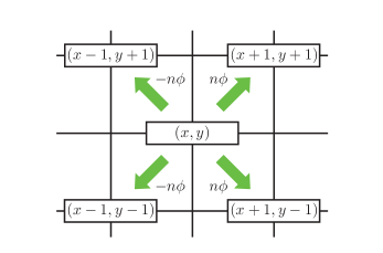
Figure 1: Applied phase modulation scheme for the nth step of the quantum walk.

In our time-multiplexed photonic quantum walk, the quantum walker state space is mapped into time delays of optical pulses. The experimental setup is a closed-loop fiber architecture composed of two beam splitters with their ports connected to fibers of different lengths mapping the $\pm x$ and $\pm y$ directions to different time delays. Full details of the experimental setup are explained in the Supplemental Material sup . One complete propagation of an optical pulse around the loop is equivalent to the hopping of the walker to one of the four possible corners in the synthetic space (Fig. 1). Semiconductor optical amplifiers as well as polarization controllers are used in the setup to compensate for the losses and polarization changes that the optical pulses experience in each round trip, respectively. The quantum walk distribution at each time step is studied via two photodetectors analyzing two channels that we refer to as the up and down channels (See Fig. S1). A single incident laser pulse that is injected into the up channel initializes the quantum walk evolution from the origin in the synthetic space.

In this setup, we use electro-optic modulators that can introduce desired phase shifts to pulses moving to the right or left directions to generate the synthetic gauge field. Specifically, here we implement a linearly time-varying gauge field ($\overrightarrow{A}=-\mathcal{E}t\hat{x}$, in which $t$ denotes the time step and $\hat{x}$ is the unit vector in the $x$ direction) that leads to the generation of a constant electric field ($\overrightarrow{\mathcal{E}}=-\partial\overrightarrow{A}/\partial t$). To implement this gauge field, a phase modulation needs to be applied that varies with the time step. Figure 1 depicts the synthetic lattice with the required phase modulation criteria describing the amount of phase that the walker accumulates in hopping to the four possible corners at time step $n$.

This method of generating an electric field is distinguished from previously used approaches in discrete-time quantum walks, which have been based on position-dependent but time-independent gauge fields Cedzich et al. (2013); Genske et al. (2013); Bru et al. (2016). In these approaches, an effective linear electric potential $V=-\mathcal{E}x$ is implemented, which leads to the generation of electric fields based on $\overrightarrow{\mathcal{E}}=-\nabla V$. In order to create such a gauge field in discrete-time quantum walks, the unitary operation in each time step must have an extra term relative to the standard quantum walk evolution operator $U_{0}$ as $U_{\phi}=e^{i\phi x}U_{0}$. In contrast, the current approach does not require any coordinate-dependent unitary operation to generate an electric field. This is of particular interest for time-multiplexed quantum walks, as it relaxes the need for any variation of phase modulations during each time step. The equivalence of these approaches can be understood in terms of a gauge transformation Cedzich et al. (2019). The similarity between the approach used and the conventional coordinate-based method of implementing an electric field in a two-dimensional quantum walk Bru et al. (2016) is described in the Supplemental Material sup . We show that the total phase accumulated in some sample closed loops that start from the origin and return to it in both pictures are the same. In fact, this similarity holds for any closed path starting from the origin and ending at it.

(a)

(b)

(c)

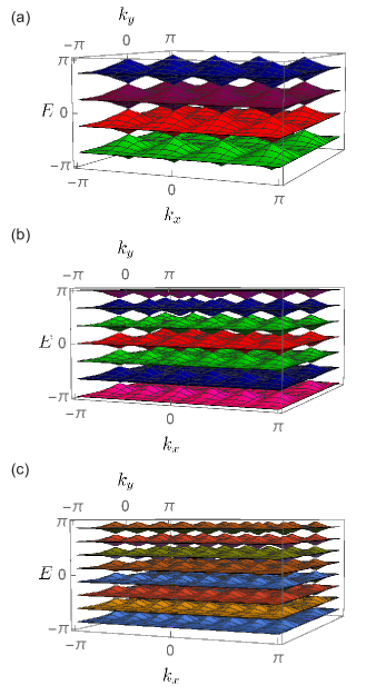
Figure 2: Pseudo energy band diagrams of the two-dimensional quantum walk for different gauge field strengths: (a) $\phi=\pi/2$, (b) $\phi=\pi/3$, and (c) $\phi=\pi/4$.

The application of the electric field in our two-dimensional discrete-time quantum walk will lead to Bloch oscillations and the revival of the quantum state. This can be intuitively explained through the band diagram structure of the system. As we show in the Supplemental Material sup , for a phase modulation with a fractional value of $\phi$ as $\phi=2\pi/q$, the band structure has $2q$ bands. The analytical expressions for the pseudo energy band structure under such a phase modulation are given by:

END

(a)

(b)

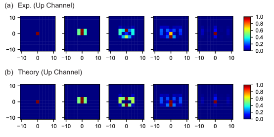
Figure 3: (a) Experimental observations and (b) theoretical predictions of the evolution of the quantum walk distribution under time-dependent phase modulation for the case of $\phi=\pi/4$. The columns from left to right show the distributions at time steps of 0, 2, 4, 6, and 8, respectively. In these plots, all the distributions are normalized to their maximum.

$$E_{n,\pm,k_{x},k_{y}}=\frac{2n\pi}{q}\pm$$

$$\frac{1}{q}\arccos\left(\cos\left(\frac{\pi q}{2}\right)\left(\sin^{q}k_{y}-1\right)-\cos\left(qk_{x}+\frac{\pi q}{2}\right)\sin^{q}k_{y}\right)$$

where $k_{x}$ and $k_{y}$ are the momentum wave vectors in inverse synthetic space and $n\in Z$. This expression for $q=1$ returns to the form of $E_{\pm}=\pm\arccos\left(\sin\left(k_{x}\right)\sin\left(k_{y}\right)\right)$, which represents the band structure for the quantum walk under no effective applied gauge field Chalabi et al. (2019). Figure 2 shows the band diagrams for three different values of the phase modulations. By increasing $q$, the band structure becomes flatter and the corresponding group velocities tend toward zero. As has been demonstrated in one dimensional quantum walks, this will lead to the revival of the quantum walk with high probability sup . This band flattening also occurs in the two-dimensional Floquet quantum walks considered here, which will lead to the return of the quantum walker toward the origin after $q$ steps. In our system, the application of an electric field in the $x$ direction will lead to the revival of the quantum walk not only in the $x$ direction but also in the $y$ direction (see Supplemental Material sup ).

To experimentally demonstrate Bloch oscillations in our 2D time-multiplexed quantum walk caused by the applied electric field, we investigate the evolution of the quantum walk distribution at different time steps. In order to measure the quantum walk distribution, we measure the power of the optical pulses received by the photodetectors at different time delays for each time step. Figure 3a shows the experimentally measured quantum walk distributions at different time steps. This figure demonstrates state revival under the application of the time-varying gauge field due to the uniform electric field generated. The phase strength of the applied electric field in this case is $\phi=\pi/4$. As this figure shows, after 8 steps, the quantum walker returns to the origin with high probability. The experimental results are in good agreement with the corresponding theoretical predictions shown in Fig. 3b.

To quantify the effect of the gauge field on the revival of the quantum state, we measure the probability of the walker returning to the origin (revival probability $P_{U}\left(0,0\right)$) as a function of the number of steps taken (Fig. 4). We measure this probability for different time-varying phase modulations after the appropriate number of time steps ($2\pi/\phi$ steps) needed for the revival to happen. As shown in Fig. 4, the revival probability increases with increasing number of steps. Additionally, this figure indicates that the experimental results are in good agreement with the theoretical predictions. In the Supplemental Material sup , we demonstrate that by decreasing the phase modulation, $\phi$, the revival probability increases and tends toward unity. Using these measured probability distributions, we can also calculate the statistical averages of the distribution at different time steps. Specifically, we measured and analyzed the quadratic means as well as the norm ones of the $x$ and $y$ coordinates at different time steps (Figs. S2 and S3). As these results show, the quadratic means as well as the norm ones of $x$ and $y$ tend toward the local minimum values after $2\pi/\phi$ steps. The variational behaviors of these quantities with the time step confirm the revival effect in both the $x$ and $y$ directions and are in good agreement with the theoretically predicted results.

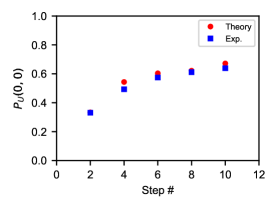
Figure 4: Probability of revival: Experimental (blue solid squares) and theoretical (red solid circles) probabilities of the walker returning to the origin with respect to the required number of quantum walker steps. The error bars in the measurements are smaller than the size of the plotted data points.

We are not restricted to implementing only uniform electric fields in our two-dimensional quantum walk. Spatially discontinuous electric fields can also be created by simply controlling the modulation pattern of the phase modulators. This provides the possibility to perform waveguiding in the synthetic space using gauge fields. Figure 5a shows an example of a discontinuous electric field in a two-dimensional synthetic space. In this configuration, the electric field is zero in the $-2<y<2$ region and non-zero outside this range. Due to the boundary created by the discontinuous gauge fields, the quantum random walk evolution is mainly confined to the region where the electric field is equal to zero. Figure 5b presents the experimentally measured quantum walk distributions at different time steps showing the trapping caused by the existence of the boundaries in the electric field pattern. The experimentally measured results are in good agreement with the theoretical predictions shown in Fig. 5c. Additionally, more quantitative agreement can be inferred based on Fig. 5d depicting the variations of the quadratic means as functions of the time step. This figure clearly shows that the presence of boundaries in the field pattern has led to the confinement of the quantum walk in the y ribbon. We note that this confinement is not induced by a bandgap and is therefore physically distinct from the confinement in conventional crystal heterostructures. None of the three regions shown in Fig. 5 supports a bandgap, thus demonstrating the confinement is directly induced by the gauge field itself. These results demonstrate the possibility of using a nonuniform electric field in order to guide the path of the quantum walk in a desired fashion.

In conclusion, we studied the time evolution of a quantum random walk under a time-varying gauge field in a two-dimensional synthetic space. Using a linearly time-varying phase modulation, an electric field acting on photonic quantum walkers can be created. Our findings demonstrate that under the influence of such an electric field a complete revival caused by Bloch oscillations happens in two-dimensional quantum walks. This revival becomes more accurate as we increase the number of steps. Moreover, we demonstrated that a discontinuous electric field could impose confinement on the evolution of a quantum random walk, even when there is no bandgap. While we demonstrated the Bloch oscillation for a quantum walk initiated with classical coherent laser pulses, the same physics holds at the single photon level. The obtained results can be extended to the investigation of the effect of dynamic localization Dunlap and Kenkre (1986); Lenz et al. (2003); Longhi et al. (2006); Iyer et al. (2007); Joushaghani et al. (2009, 2012); Yuan and Fan (2015). Our demonstration of an electric field for photons in time-multiplexed synthetic lattices will have potential applications in photonic quantum simulations, for example, multi-photon interference and Boson sampling in the time-domain Orre et al. (2019), and the realization of photonic lattices with strong nonlinearities mediated via artificial atoms like quantum dots Pichler et al. (2017); Chalabi and Waks (2018).

This work was supported by the Air Force Office of Scientific Research-Multidisciplinary University Research Initiative (Grant No. FA9550-16-1-0323), the Physics Frontier Center at the Joint Quantum Institute, the National Science Foundation (Grant No. PHYS. 1415458 as well as PHY-1430094), and the Center for Distributed Quantum Information. The authors would also like to acknowledge support from the U.S. Department of Defense. Moreover, the authors acknowledge support from the Laboratory for Telecommunication Sciences.

END

(a)

(b)

(c)

(d)

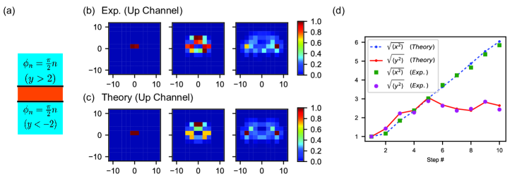
Figure 5: Confinement of the quantum walker through the application of a discontinuous electric field. (a) Schematic describing the phase modulation pattern in the synthetic space that leads to a zero electric field for $-2<y<2$ and a non-zero electric field outside this range (b) Experimental observations and (c) theoretical predictions of the evolution of the quantum walk distribution under the discontinuous electric field. The columns from left to right show the distributions at time steps of 1, 5, and 9, respectively. All the distributions are normalized to their maximum. (d) Experimentally measured and theoretically predicted quadratic means of x and y as a function of the time step. The error bars in the measurements are smaller than the size of the plotted data points.

END

in 1,…,20 See pages \x of SupplemMaterial

References

- Sparrow et al. (2018) C. Sparrow, E. Martín-López, N. Maraviglia, A. Neville, C. Harrold, J. Carolan, Y. N. Joglekar, T. Hashimoto, N. Matsuda, J. L. O’Brien, D. P. Tew, and A. Laing, Nature 557, 660 (2018).
- Ma et al. (2011) X.-s. Ma, B. Dakic, W. Naylor, A. Zeilinger, and P. Walther, Nature Physics 7, 399 (2011).
- Lanyon et al. (2010) B. P. Lanyon, J. D. Whitfield, G. G. Gillett, M. E. Goggin, M. P. Almeida, I. Kassal, J. D. Biamonte, M. Mohseni, B. J. Powell, M. Barbieri, A. Aspuru-Guzik, and A. G. White, Nature Chemistry 2, 106 (2010).
- Aspuru-Guzik and Walther (2012) A. Aspuru-Guzik and P. Walther, Nature Physics 8, 285 (2012).
- Navarrete-Benlloch et al. (2007) C. Navarrete-Benlloch, A. Pérez, and E. Roldán, Physical Review A 75, 062333 (2007).
- Bouwmeester et al. (1999) D. Bouwmeester, I. Marzoli, G. P. Karman, W. Schleich, and J. P. Woerdman, Physical Review A 61, 013410 (1999).
- Bell et al. (2017) B. A. Bell, K. Wang, A. S. Solntsev, D. N. Neshev, A. A. Sukhorukov, and B. J. Eggleton, Optica 4, 1433 (2017).
- Qin et al. (2018) C. Qin, F. Zhou, Y. Peng, D. Sounas, X. Zhu, B. Wang, J. Dong, X. Zhang, A. Alù, and P. Lu, Physical Review Letters 120, 133901 (2018).
- Dutt et al. (2019) A. Dutt, M. Minkov, Q. Lin, L. Yuan, D. A. B. Miller, and S. Fan, Nature Communications 10, 3122 (2019), arXiv:1903.07842 .
- Regensburger et al. (2012) A. Regensburger, C. Bersch, M.-A. Miri, G. Onishchukov, D. N. Christodoulides, and U. Peschel, Nature 488, 167 (2012).
- Lustig et al. (2019) E. Lustig, S. Weimann, Y. Plotnik, Y. Lumer, M. A. Bandres, A. Szameit, and M. Segev, Nature 567, 356 (2019).
- Lin et al. (2016) Q. Lin, M. Xiao, L. Yuan, and S. Fan, Nature Communications 7, 13731 (2016).
- Lin et al. (2018) Q. Lin, X.-Q. Sun, M. Xiao, S.-C. Zhang, and S. Fan, Science Advances 4, eaat2774 (2018).
- Yuan et al. (2018) L. Yuan, M. Xiao, Q. Lin, and S. Fan, Physical Review B 97, 104105 (2018), arXiv:1710.01373 .
- Goyal et al. (2013) S. K. Goyal, F. S. Roux, A. Forbes, and T. Konrad, Physical Review Letters 110, 263602 (2013).
- Cardano et al. (2015) F. Cardano, F. Massa, H. Qassim, E. Karimi, S. Slussarenko, D. Paparo, C. de Lisio, F. Sciarrino, E. Santamato, R. W. Boyd, and L. Marrucci, Science Advances 1, e1500087 (2015).
- Cardano et al. (2016) F. Cardano, M. Maffei, F. Massa, B. Piccirillo, C. de Lisio, G. De Filippis, V. Cataudella, E. Santamato, and L. Marrucci, Nature Communications 7, 11439 (2016).
- Cardano et al. (2017) F. Cardano, A. D’Errico, A. Dauphin, M. Maffei, B. Piccirillo, C. de Lisio, G. De Filippis, V. Cataudella, E. Santamato, L. Marrucci, M. Lewenstein, and P. Massignan, Nature Communications 8, 15516 (2017).
- Schreiber et al. (2010) A. Schreiber, K. N. Cassemiro, V. Potoček, A. Gábris, P. J. Mosley, E. Andersson, I. Jex, and C. Silberhorn, Physical Review Letters 104, 050502 (2010).
- Schreiber et al. (2011) A. Schreiber, K. N. Cassemiro, V. Potoček, A. Gábris, I. Jex, and C. Silberhorn, Physical Review Letters 106, 180403 (2011).
- Schreiber et al. (2012) A. Schreiber, A. Gabris, P. P. Rohde, K. Laiho, M. Stefanak, V. Potocek, C. Hamilton, I. Jex, and C. Silberhorn, Science 336, 55 (2012).
- Nitsche et al. (2016) T. Nitsche, F. Elster, J. Novotný, A. Gábris, I. Jex, S. Barkhofen, and C. Silberhorn, New Journal of Physics 18, 063017 (2016).
- Barkhofen et al. (2017) S. Barkhofen, T. Nitsche, F. Elster, L. Lorz, A. Gábris, I. Jex, and C. Silberhorn, Physical Review A 96, 033846 (2017).
- Chen et al. (2018) C. Chen, X. Ding, J. Qin, Y. He, Y.-H. Luo, M.-C. Chen, C. Liu, X.-L. Wang, W.-J. Zhang, H. Li, L.-X. You, Z. Wang, D.-W. Wang, B. C. Sanders, C.-Y. Lu, and J.-W. Pan, Physical Review Letters 121, 100502 (2018).
- Hafezi et al. (2011) M. Hafezi, E. A. Demler, M. D. Lukin, and J. M. Taylor, Nature Physics 7, 907 (2011).
- Mittal et al. (2014) S. Mittal, J. Fan, S. Faez, A. Migdall, J. M. Taylor, and M. Hafezi, Physical Review Letters 113, 087403 (2014).
- Rechtsman et al. (2013) M. C. Rechtsman, J. M. Zeuner, Y. Plotnik, Y. Lumer, D. Podolsky, F. Dreisow, S. Nolte, M. Segev, and A. Szameit, Nature 496, 196 (2013).
- Fang et al. (2012) K. Fang, Z. Yu, and S. Fan, Nature Photonics 6, 782 (2012).
- Ozawa et al. (2019) T. Ozawa, H. M. Price, A. Amo, N. Goldman, M. Hafezi, L. Lu, M. C. Rechtsman, D. Schuster, J. Simon, O. Zilberberg, and I. Carusotto, Reviews of Modern Physics 91, 015006 (2019).
- Hu et al. (2015) W. Hu, J. C. Pillay, K. Wu, M. Pasek, P. P. Shum, and Y. D. Chong, Physical Review X 5, 011012 (2015).
- D’Errico et al. (2018) A. D’Errico, F. Cardano, M. Maffei, A. Dauphin, R. Barboza, C. Esposito, B. Piccirillo, M. Lewenstein, P. Massignan, and L. Marrucci, “Two-dimensional topological quantum walks in the momentum space of structured light,” (2018), arXiv:1811.04001 [quant-ph] .
- Bromberg et al. (2010) Y. Bromberg, Y. Lahini, and Y. Silberberg, Physical Review Letters 105, 263604 (2010).
- Corrielli et al. (2013) G. Corrielli, A. Crespi, G. Della Valle, S. Longhi, and R. Osellame, Nature Communications 4, 1555 (2013).
- Witthaut et al. (2004) D. Witthaut, F. Keck, H. J. Korsch, and S. Mossmann, New Journal of Physics 6, 41 (2004).
- Bloch (1929) F. Bloch, Zeitschrift fï¿œr Physik 52, 555 (1929).
- Haller et al. (2010) E. Haller, R. Hart, M. J. Mark, J. G. Danzl, L. Reichsöllner, and H.-C. Nägerl, Physical Review Letters 104, 200403 (2010).
- Ben Dahan et al. (1996) M. Ben Dahan, E. Peik, J. Reichel, Y. Castin, and C. Salomon, Physical Review Letters 76, 4508 (1996).
- Pertsch et al. (1999) T. Pertsch, P. Dannberg, W. Elflein, A. Bräuer, and F. Lederer, Physical Review Letters 83, 4752 (1999).
- Morandotti et al. (1999) R. Morandotti, U. Peschel, J. S. Aitchison, H. S. Eisenberg, and Y. Silberberg, Physical Review Letters 83, 4756 (1999).
- Lenz et al. (1999) G. Lenz, I. Talanina, and C. M. de Sterke, Physical Review Letters 83, 963 (1999).
- Trompeter et al. (2006) H. Trompeter, W. Krolikowski, D. N. Neshev, A. S. Desyatnikov, A. A. Sukhorukov, Y. S. Kivshar, T. Pertsch, U. Peschel, and F. Lederer, Physical Review Letters 96, 053903 (2006).
- Longhi (2006) S. Longhi, Europhysics Letters (EPL) 76, 416 (2006).
- Dreisow et al. (2009) F. Dreisow, A. Szameit, M. Heinrich, T. Pertsch, S. Nolte, A. Tünnermann, and S. Longhi, Physical Review Letters 102, 076802 (2009).
- Levy and Kumar (2010) M. Levy and P. Kumar, Optics Letters 35, 3147 (2010).
- Xue et al. (2015) P. Xue, R. Zhang, H. Qin, X. Zhan, Z. H. Bian, J. Li, and B. C. Sanders, Physical Review Letters 114, 140502 (2015).
- Cedzich and Werner (2016) C. Cedzich and R. F. Werner, Physical Review A 93, 032329 (2016).
- Peschel et al. (2008) U. Peschel, C. Bersch, and G. Onishchukov, Open Physics 6 (2008), 10.2478/s11534-008-0095-0.
- Bersch et al. (2009) C. Bersch, G. Onishchukov, and U. Peschel, Optics Letters 34, 2372 (2009).
- Yuan and Fan (2016) L. Yuan and S. Fan, Optica 3, 1014 (2016).
- (50) See Supplemental Material at [URL will be inserted by publisher] for methods and theoretical derivations.
- Cedzich et al. (2013) C. Cedzich, T. Rybár, A. H. Werner, A. Alberti, M. Genske, and R. F. Werner, Physical Review Letters 111, 160601 (2013), arXiv:1302.2081 .
- Genske et al. (2013) M. Genske, W. Alt, A. Steffen, A. H. Werner, R. F. Werner, D. Meschede, and A. Alberti, Physical Review Letters 110, 190601 (2013).
- Bru et al. (2016) L. A. Bru, M. Hinarejos, F. Silva, G. J. de Valcárcel, and E. Roldán, Physical Review A 93, 032333 (2016).
- Cedzich et al. (2019) C. Cedzich, T. Geib, A. H. Werner, and R. F. Werner, Journal of Mathematical Physics 60, 012107 (2019), arXiv:1808.10850 .
- Chalabi et al. (2019) H. Chalabi, S. Barik, S. Mittal, T. E. Murphy, M. Hafezi, and E. Waks, Physical Review Letters 123, 150503 (2019).
- Dunlap and Kenkre (1986) D. H. Dunlap and V. M. Kenkre, Physical Review B 34, 3625 (1986).
- Lenz et al. (2003) G. Lenz, R. Parker, M. Wanke, and C. de Sterke, Optics Communications 218, 87 (2003).
- Longhi et al. (2006) S. Longhi, M. Marangoni, M. Lobino, R. Ramponi, P. Laporta, E. Cianci, and V. Foglietti, Physical Review Letters 96, 243901 (2006).
- Iyer et al. (2007) R. Iyer, J. Stewart Aitchison, J. Wan, M. M. Dignam, and C. Martijn de Sterke, Optics Express 15, 3212 (2007).
- Joushaghani et al. (2009) A. Joushaghani, R. Iyer, J. K. S. Poon, J. S. Aitchison, C. M. de Sterke, J. Wan, and M. M. Dignam, Physical Review Letters 103, 143903 (2009).
- Joushaghani et al. (2012) A. Joushaghani, R. Iyer, J. K. S. Poon, J. S. Aitchison, C. M. de Sterke, J. Wan, and M. M. Dignam, Physical Review Letters 109, 103901 (2012).
- Yuan and Fan (2015) L. Yuan and S. Fan, Physical Review Letters 114, 243901 (2015).
- Orre et al. (2019) V. V. Orre, E. A. Goldschmidt, A. Deshpande, A. V. Gorshkov, V. Tamma, M. Hafezi, and S. Mittal, Physical Review Letters 123, 123603 (2019).
- Pichler et al. (2017) H. Pichler, S. Choi, P. Zoller, and M. D. Lukin, Proceedings of the National Academy of Sciences 114, 11362 (2017).
- Chalabi and Waks (2018) H. Chalabi and E. Waks, Physical Review A 98, 063832 (2018).