Theory of the coherence of topological lasers

Abstract

We present a theoretical study of the temporal and spatial coherence properties of a topological laser device built by including saturable gain on the edge sites of a Harper–Hofstadter lattice for photons. For small enough lattices the Bogoliubov analysis applies, the emission is nearly a single-mode one and the coherence time is almost determined by the total number of photons in the device in agereement with the standard Schawlow-Townes phase diffusion. In larger lattices, looking at the lasing edge mode in the comoving frame of its chiral motion, the spatio-temporal correlations of long-wavelength fluctuations display a Kardar-Parisi-Zhang (KPZ) scaling. Still, at very long times, when the finite size of the device starts to matter, the functional form of the temporal decay of coherence changes from the KPZ stretched exponential to a Schawlow-Townes-like exponential, while the nonlinear many-mode dynamics of KPZ fluctuations remains visible as an enhanced linewidth as compared to the single-mode Schawlow-Townes prediction. While we have established the above behaviors also for non-topological laser arrays, the crucial role of topology in protecting the coherence from static disorder is finally highlighted: our ground-breaking numerical calculations suggest the dramatically reinforced coherence properties of topological lasers compared to corresponding non-topological devices. These results open exciting possibilities for both fundamental studies of non-equilibrium statistical mechanics and concrete applications to laser devices.

I Introduction

The laser is one of the most fundamental tools in modern science (Siegman, 1987; Svelto, 2010). Its defining feature is the emission of radiation with unprecedented long coherence length and time. This makes laser sources essential ingredients in a wide range of applications and justifies the continuous theoretical and technological research of new devices. Also from a fundamental science perspectives, the physical mechanisms underlying laser oscillation represent an archetypical model at the crossroad of nonlinear physics, non-equilibrium statistical mechanics, and quantum optics Haken (1983); Gardiner and Zoller (2004); Chiocchetta et al. (2017); Keeling et al. (2017).

Recent years have witnessed an explosion of the field of topological photonics (Ozawa et al., 2019). Following the ground-breaking works Haldane and Raghu (2008); Wang et al. (2009), experiments have initially focussed on demonstrating the topologically protected chiral propagation of light along the edges of passive photonic lattices displaying topologically non-trivial band structures in a variety of different material platforms and frequency regions. In addition to the study of nonlinear topological photonics effects Smirnova et al. (2019), a major attention has been devoted in the last years to laser operation in topological edge modes Ota et al. (2020), first in one-dimensional SSH chains of polariton resonators (St-Jean et al., 2017) and, soon afterwards, in 2D photonic crystal (Bahari et al., 2017) and microcavity arrays (Bandres et al., 2018).

Pioneering theoretical studies have focused on the properties of the steady-state emission of topological laser devices (Harari et al., 2018; Seclì et al., 2019), highlighting their promise with respect to the power slope efficiency and to the robustness of the steady state emission in the presence of a strong static defect located on the edge of the lattice or of a moderate disorder distributed throughout the device. However, a dynamical study of the temporal and spatial coherence properties of the resulting laser emission including the effect of noise due, e.g., to spontaneous emission is still missing. The characterization of the ultimate limitations to the coherence properties is a key element in view of technological applications of topological lasers and will be the main topic of this work.

In the absence of external noise sources, the long time coherence of a single-mode laser is ruled by the diffusion of the phase of the macroscopic electromagnetic field. As it was first theoretically understood by Schawlow and Townes (Schawlow and Townes, 1958), an intrinsic mechanism for the diffusion of the phase is given by spontaneous emission events, which result in an exponential decay of the temporal coherence function and in a corresponding broadening of the emission linewidth. In analogy with this ultimate linewidth of single-mode lasers, it is natural to investigate the ultimate limitations to the coherence of a spatially extended topological laser device whose physics involves a complex multi-mode nonlinear dynamics, to be treated with non-equilibrium statistical mechanics methods.

To facilitate the identification of the fundamental process common to all concrete realizations of topological laser device, we restrict to the simplest scenario of a so-called class-A laser Longhi et al. (2018), in which the carrier dynamics in the gain medium can be neglected and laser operation is described in terms of a coherent field amplified by a saturable gain medium with a temporally instantaneous response. With no loss of generality, we focus on the Harper–Hofstadter topological laser model and we consider that gain is distributed around the whole edge of the system (Seclì et al., 2019). We further assume that the real part of the refractive index of the medium does not depend on light intensity. As usual in the semi-classical laser theory Gardiner and Zoller (2004); Scully and Zubairy (1997), the effect of spontaneous emission is modeled as a spatio-temporally white noise in the stochastic differential equations for the multi-mode laser field.

Since topological laser operation occurs into a chiral mode localized on the one-dimensional edge of the two-dimensional lattice, we expect that the coherence properties resemble the ones of one-dimensional arrays of coupled laser resonators, for which it was anticipated in (Gladilin et al., 2014; Altman et al., 2015; Ji et al., 2015; He et al., 2015; Lauter et al., 2017; Squizzato et al., 2018) that (for small intensity fluctuations) the long–wavelength phase dynamics follows a Kardar-Parisi-Zhang (KPZ) dynamics (Kardar et al., 1986) Here, we numerically prove that the same holds for the topological laser, once the phase fluctuations are studied in the reference frame moving at the group velocity of the chiral mode. In particular, we show that the spatio-temporal correlation functions satisfy the KPZ scaling with no dramatic renormalization of the nonlinear coupling.

While the KPZ scaling holds in spatially infinite systems or, in finite systems, until the dynamics has had time to experience the finite size, the study of key optical properties such as long-time coherence of a realistic topological laser device requires an explicit analysis of finite-size effects that goes beyond the available non-equilibrium statistical mechanics literature. In this respect, a main result of our study is that the very long time coherence of a finite system does not follow the KPZ scaling but decays exponentially à la Schawlow-Townes, yet with a reinforced phase diffusion coefficient due to the intrinsic nonlinearity of the KPZ model. For smaller lattices instead, the Bogoliubov analysis applies and yields a Petermann factor Siegman (1989a, b) close to unity, meaning that the emission is nearly single-mode and, in agreement with the standard Schawlow-Townes picture, its coherence time is determined by the total number of photons in the device over the noise rate, which is the optimal scenario.

Finally, as a dramatic consequence of the topological protection, our ground-breaking numerical simulations suggest that coherence of a topological laser is very weakly affected by a static disorder. Coherence is only lost when the strength of disorder is on the order of the topological gap, that is orders of magnitude higher than what is needed to spoil the coherence of a non-topological array. This has a paramount importance in view of practical applications of topological lasers as sources of intense coherent light.

The structure of the article is the following. In Sec. II we focus on finite 1D laser chains and, after inspecting the crossover from the Kardar-Parisi-Zhang scaling to a Schawlow-Townes-like phase diffusion at very long times, we illustrate the significant reduction of the coherence time from the single-mode Schawlow–Townes prediction due to the nonlinear dynamics of the spatial fluctuations of the phase. In Sec. III we first review the basic concepts of topological laser operation into the chiral edge mode of a 2D Harper–Hofstadter lattice. We then investigate the emission spectrum and the one–dimensional character of the phase fluctuations. In particular, we probe the universal KPZ scaling of long wavelength fluctuations at intermediate times and we compute the linewidth of the laser emission at very long times. In Sec. IV we demonstrate the robustness of the coherence of the topological laser emission in the presence of a static disorder. Conclusions and perspectives are finally drawn in Section V.

II One-dimensional array of laser resonators

In this Section we make use of a semi-classical approach based on stochastic differential equations to characterize the coherence properties of a simple model of spatially extended laser formed by a one-dimensional array of single-mode resonators. While a sizable literature has investigated the behaviour of long-wavelength fluctuations in terms of the KPZ equation (Altman et al., 2015; Gladilin et al., 2014; Ji et al., 2015; He et al., 2015; Lauter et al., 2017; Squizzato et al., 2018), not much attention has been paid to the temporal dependence of the equal–space correlation function of spatially finite systems, which is one of the experimentally most relevant quantities for lasers. To facilitate the reader, we will first set the stage by reviewing the Schawlow–Townes linewidth for single laser resonators and then we will move up to the case of interest of a finite array of coupled resonators.

II.1 Single resonator linewidth

The basic features of laser operation in a single-mode resonator, namely stimulated amplification, the spontaneous breaking of the $U(1)$ symmetry of the field and the stabilization of the emission intensity by gain saturation are all captured by the stochastic differential equation

$$i\partial_{t}\psi=\frac{i}{2}\left[\frac{P}{1+n/n_{S}}-\gamma\right]\psi+\sqrt{2D}\xi\ ,$$ (1)

for the single complex variable $\psi$ describing the amplitude of the electromagnetic field in the resonator, $n=|\psi|^{2}$ is the field intensity, $\gamma$ is the loss rate of the “cold” resonator, $P$ the amplification rate induced by the (unsaturated) gain and $n_{S}$ is the gain saturation coefficient. The stochastic term $\xi$ consists of a white noise of unit variance $\langle\xi^{*}(t)\xi(t^{\prime})\rangle=\delta(t-t^{\prime})$ rescaled to have a diffusion coefficient $D$.

Eq. (1) is invariant under a $U(1)$ symmetry describing the rotation of the phase of the field $\psi$. The steady–state field $\psi_{0}$ is zero below the lasing threshold $P<P_{th}=\gamma$. Above the threshold $P>P_{th}$, it breaks the symmetry by choosing a specific phase and the steady-state intensity $n_{0}$ satisfies $n_{0}=n_{S}\left[\frac{P}{P_{th}}-1\right]$. In particular, for $P=2P_{th}$ it holds the very transparent expression $n_{0}=n_{S}$.

To deal analytically with Eq. (1) it is convenient to resort to the modulus–phase formalism: writing the field as $\psi=\sqrt{n}e^{i\phi}$ one has

$$\partial_{t}\phi = \sqrt{\frac{D}{n}}\xi_{1}$$ (2)

$$\partial_{t}n = \left[\frac{P}{1+n/n_{S}}-\gamma\right]n+2\sqrt{nD}\ \xi_{2}$$ (3)

in terms of the two real and independent noises $\langle\xi_{l}(t)\xi_{l^{\prime}}(t^{\prime})\rangle=\delta_{l,l^{\prime}}\delta(t-t^{\prime}),\ l,l^{\prime}=1,2$. For small enough perturbations, the intensity relaxes to $n_{0}$ with at a rate $\Gamma=\frac{\gamma(P-\gamma)}{P}$. On the other hand, as a direct consequence of the $U(1)$ symmetry of the model, the dynamics of the phase is a diffusion with no restoring force.

Assuming noise is small enough to cause minor perturbations to the intensity, phase differences follow a Gaussian distribution, so within the so-called cumulant approximation (Gladilin et al., 2014), the autocorrelation of the field reads

$$g^{(1)}(t)=\langle\psi^{*}(t)\psi(0)\rangle\simeq n_{0}e^{-\frac{1}{2}\langle[\phi(t)-\phi(0)]^{2}\rangle}.$$ (4)

As a consequence, the usual Brownian motion scaling entails that the decay of coherence is described by the exponential

$$g^{(1)}(t)\simeq n_{0}e^{-\frac{\gamma_{ST}}{2}|t|}.$$ (5)

In Fourier space, this corresponds to a Lorentzian power spectral density. The coherence decay rate

$$\gamma_{ST}=\frac{D}{n_{0}}.$$ (6)

is the celebrated Schawlow–Townes linewidth Schawlow and Townes (1958); Henry (1982). The crucial feature of this formula is the steady-state intensity $n_{0}$ appearing at the denominator, which has the following physical interpretation: the more photons are present in the resonator, the less the phase of the field is perturbed when a additional photon with a random phase is emitted into the mode by a spontaneous emission process.

II.2 Extended lasers and KPZ equation

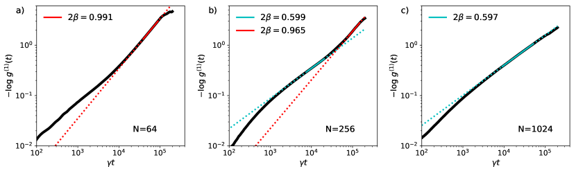
Figure 1: Kardar-Parisi-Zhang to Schawlow-Townes crossover in the temporal coherence of finite, one-dimensional laser arrays The numerical prediction of Eq. (7) for the logarithm of the equal–space time correlation function $-\log g^{(1)}(t)$ is plotted in loglog scale as a function of time for increasing system sizes $N_{x}=64$ (left), $N_{x}=256$ (middle), $N_{x}=1024$ (right). In all cases, lasing occurs around $k_{x}^{las}=0$. For a given temporal window, the decay of the coherence is dominated by a Schawlow–Townes–like diffusion $g^{(1)}(t)\sim e^{-B|t|}$ for small sizes [panel (a)] and by the KPZ behavior $g^{(1)}(t)\sim e^{-B|t|^{2/3}}$ for large sizes [panel (c)]. The crossover between the two regimes is visible for intermediate sizes [panel (b)]. The cyan and red lines are linear fits of $\log[-\log g^{(1)}(t)]$ with $2\beta\log|t|+B^{\prime}$. Other system parameters: $J=0.5\gamma$, $P=2\gamma$, $n_{S}=1000,D=\gamma$.

For a single single-mode resonator, the linewidth is inversely proportional to the number of photons present in the mode. For an array of coupled resonators, the naive intuition is that the linewidth will be determined by the number of photons that are present within some correlation length. In particular, for small system sizes all resonators oscillate in phase and, for a given number of photons per resonator $n_{0}$, the coherence time is proportional to length of the array. On the other hand, for large enough systems, it is known that the physics is described by the Kardar–Parisi–Zhang (KPZ) equation(He et al., 2015). The main goal of this Section is to connect these two points of view into a unified perspective.

To attack this question in a quantitative way, we make use of a generalization of Eq. (1) to a one–dimensional array of $N_{x}$ coupled laser resonators $x=1,...,N_{x}$

$$i\partial_{t}\psi_{x}=-J\psi_{x+1}-J\psi_{x-1}+\frac{i}{2}\left[\frac{P}{1+\frac{n_{x}}{n_{S}}}-\gamma\right]\psi_{x}+\sqrt{2D}\xi_{x}\ ,$$ (7)

with inter-site coupling $J$ and independent noises $\langle\xi_{x}^{*}(t)\xi_{x^{\prime}}(t^{\prime})\rangle=\delta_{xx^{\prime}}\delta(t-t^{\prime})$. Periodic boundary conditions are assumed.

For large $J$ and calling $a$ the distance between neighbouring resonators, one can interpret Eq. (7) as a discrete version of a continuous field of mass $m=\frac{1}{2Ja^{2}}$. The corresponding continuous equation is the complex Ginzburg–Landau equation (Wouters and Carusotto, 2007). Assuming fast relaxation of the intensity fluctuations, one can focus on the dynamics of the phase (derivation reviewed in Sec. SI sup ), which is described by the Kuramoto–Sivashinsky equation (KSE)

$$\partial_{{t}}{\phi}=\frac{1}{2m}\left[-\frac{\Gamma^{-1}}{2m}\partial^{4}_{{x}}{\phi}-(\partial_{{x}}{\phi})^{2}\right]+\sqrt{\frac{D}{n_{0}}}{\xi_{1}}.$$ (8)

Here, $\phi$ is the unwound phase living on the real axis, and not the compact one restricted to $[0,2\pi]$.

The characteristic scales of the system as a function of the microscopic parameters have been reported in Gladilin et al. (2014):

$$l^{*}=\left[\frac{J^{4}}{\Gamma^{3}Dn_{0}^{-1}}\right]^{1/7},\ \ t^{*}=\left[\frac{J^{2}}{\Gamma^{5}(Dn_{0}^{-1})^{4}}\right]^{1/7},$$

$$\ \ \phi^{*}=\left[\frac{(Dn_{0}^{-1})^{2}}{J\Gamma}\right]^{1/7}.$$ (9)

Measuring space, time and (unwound) phase in terms of $l^{*},t^{*},\phi^{*}$ the adimensional KSE reads

$$\partial_{\tilde{t}}\tilde{\phi}=-\partial^{4}_{\tilde{x}}\tilde{\phi}-(\partial_{\tilde{x}}\tilde{\phi})^{2}+\tilde{\xi}.$$ (10)

However, since other scales can be relevant for the $2D$ topological laser to be discussed below, in most of the paper we will use the physical (without tilde) space, time and phase variables. A rescaling will be proposed in order to study KPZ features in Sec. III.4.

The renormalization group analysis shows that at long distances and times the KSE flows to the KPZ universality class(Ueno et al., 2005). The KPZ equation (Kardar et al., 1986) reads

$$\partial_{\tilde{t}}\tilde{\phi}=\nu\partial^{2}_{\tilde{x}}\tilde{\phi}+\frac{\lambda}{2}(\partial_{\tilde{x}}\tilde{\phi})^{2}+\sqrt{\mathcal{D}}{\xi_{1}}$$ (11)

and it was originally proposed to describe the growth of interfaces. Its scaling behavior at low energies (and assuming an infinite system and stationary regime) is characterized by the correlation function

$$\Delta\tilde{\phi}_{\tilde{x},\tilde{t}}^{2}\equiv\langle[\tilde{\phi}(\tilde{x},\tilde{t})-\tilde{\phi}(0,0)]^{2}\rangle$$ (12)

and by two exponents $\chi,z$ which determine the asymptotic behavior of the spatial and temporal correlations respectively, according to $\Delta\tilde{\phi}_{\tilde{x},0}^{2}\sim\tilde{x}^{2\chi}$ and $\Delta\tilde{\phi}_{0,\tilde{t}}^{2}\sim\tilde{t}^{2\chi/z}$. In $1D$ we have $\chi=1/2$ for the roughness exponent and $z=3/2$ for the dynamical exponent; even more precisely it holds

$$\Delta\tilde{\phi}_{\tilde{x},\tilde{t}}^{2}=\left(\frac{1}{2}\lambda A^{2}t\right)^{2/3}g_{KPZ}\left(\frac{\tilde{x}}{(2\lambda^{2}A\tilde{t}^{2})^{1/3}}\right)$$ (13)

where $A=\mathcal{D}/\nu$ is the variance of $\partial_{\tilde{x}}\tilde{\phi}$. The universal function $g_{KPZ}$ is known exactly (Prähofer and Spohn, 2004) and we here recall its limiting values $g_{KPZ}(u)-2|u|\to 0$ for $u\to\infty$ and $g_{KPZ}(u)\to 1.150...$ for $u\to 0$.

As a consequence, the equal–time correlation function has the random walk form $\Delta\tilde{\phi}_{\tilde{x},0}^{2}=\frac{A}{2}|\tilde{x}|$, for which the KPZ nonlinearity $\lambda$ does not play any role. In other words, only looking at the spatial correlations the dynamics is not distinguishable from the one of the linear ($\lambda=0$) Edwards–Wilkinson (EW) model. In both cases, one has $\chi=1/2$ which corresponds to an exponential decay of the spatial coherence Gladilin et al. (2014); He et al. (2015).

A difference is instead visible in the spatio-temporal correlations, which have $z=2$ in the linear EW model and $z=3/2$ in KPZ. In fact, at small distances and times, the nonlinear term in the KSE can be neglected and a linearized Bogoliubov analysis is accurate. A numerical illustration of the collapse of the coherence functions to the scaling form (13) will be given later on in Fig.6(b) in comparison with the topological lasing case. Even though it goes beyond the present work, it is interesting to remind that the crossover from EW to KPZ physics was shown in Ji et al. (2015) to be slower in the presence of a nonlinear refractive index.

II.3 Linewidth of extended lasers

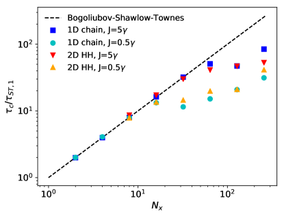
Figure 2: Scaling of the coherence time with system size $N_{x}$. The coherence time $\tau_{c}$ is extracted from the long-time exponential decay of coherence for different systems. Blue and cyan markers refer to the one-dimensional, topologically trivial arrays of laser resonators of Eq. (7) with different values of the inter-site coupling $J=5\gamma$ and $J=0.5\gamma$. The red and orange markers refer to the topological laser case of Eq. (20) for the same two values of $J$. For each point, the value of the coherence time $\tau_{c}$ is normalized to the single-site coherence time $\tau_{ST,1}\equiv\tau_{ST}/N_{x}$ where $\tau_{ST}$ is the Bogoliubov–Schawlow-Townes prediction [(16) for the trivial and (32) for the topological device].

The KPZ results reviewed in the previous sub-section apply to spatially infinite systems in the long-time limit, but are not of direct applicability to the concrete problem of the emission linewidth of a realistic laser device which necessarily has a finite spatial extension. To this purpose, the crucial quantity to study is the time dependence of the equal–space correlator

$$g^{(1)}(t)=\frac{1}{n_{0}}\left|\langle\psi^{*}(x,t)\psi(x,0)\rangle\right|,$$ (14)

which characterizes the temporal coherence of the emission. The dependence on $x$ has been dropped since we are considering a spatially uniform system.

II.3.1 Linearized Bogoliubov prediction

In the Bogoliubov limit, where the linearization on top of the noiseless state is a good approximation, modes of different momenta are decoupled. For a discrete lattice, one obtains with simple algebra that

$$\langle[\phi(x,t)-\phi(x,0)]^{2}\rangle=\frac{1}{N_{x}}\sum_{x}\langle[\phi(x,t)-\phi(x,0)]^{2}\rangle=\\ =\frac{1}{n_{0}N_{x}}\sum_{k}\bar{D}_{k}\int_{0}^{t}dt^{\prime}e^{-2i\omega_{k}(t-t^{\prime})}.$$ (15)

where the effective drift coefficients $\bar{D}_{k}$ are determined by the shape of the Bogoliubov modes and tend to $D$ in the long-wavelength limit $k\to 0$. In this same limit, the lowest Bogoliubov mode has a diffusive character with $\omega_{k}\simeq-i\gamma_{k}=-iJ^{2}\Gamma^{-1}k^{4}$ Wouters and Carusotto (2007). The factor $1/N_{x}$ in front of (15) can be interpreted by viewing the white spatial noise as randomly drawing noise realizations with a given $k$ and unit strength at each site. The probability to pick a given mode is then $1/N_{x}$.

In a spatially finite system where $k$ is quantized, only the $k=0$ mode gives a finite contribution at long times, proportional to $|t|$; the contribution of all other modes decays instead exponentially with time. From this, one immediately obtains the expression of the Bogoliubov–Schawlow–Townes coherence time

$$\tau_{c}=\tau_{ST}=2\gamma_{ST}^{-1}=\frac{2n_{0}N_{x}}{D}$$ (16)

that generalizes the Schawlow-Townes phase diffusion to the case of a finite laser array, $n_{0}N_{x}$ being equal to the total number of photons.

The situation is a bit different for an infinite array. In this case, the sum over discrete $k$ modes has to be replaced by an integral $k$. This yield  the Bogoliubov prediction $g^{(1)}(t)\sim e^{-B|t|^{3/4}}$, where $B$ is a constant. The slower power-law decay stems from the fact that the specific $k=0$ mode is now occurring with a probability zero.

For the sake of completeness, it is worth noting that a different scaling would be found in the presence of a nonlinear refractive index. In this case, the imaginary part of the Bogoliubov frequency scales in fact as $\gamma_{k}\propto k^{2}$ Wouters and Carusotto (2007), which leads to $g^{(1)}(t)\sim e^{-B|t|^{1/2}}$ for an infinite one-dimensional system.

II.3.2 Nonlinear KPZ effects

All the results discussed in the previous subsection were based on a linearized Bogoliubov approximation where different modes are decoupled. Of course, we know that this approximation is not adequate for an infinite or large enough system, where nonlinear KPZ features set in. For an infinite system a stretched exponential behavior

$$g^{(1)}(t)\sim e^{-B|t|^{2\beta}}$$ (17)

was predicted in (He et al., 2015), with a universal $2\beta=2\chi/z=2/3$ and a non–universal value of the constant $B$.

If the system is sufficiently large but finite, the Bogoliubov approximation breaks down, but the spontaneously broken $U(1)$ symmetry still imposes that the coherence must decay at long times at least as fast as a pure exponential, $g^{(1)}(t)\sim e^{-|t|/\tau_{c}}$. In this case, we expect that the KPZ physics typical of the infinite chain should remain visible only for intermediate times, up to a saturation time scaling as $(N_{x})^{z}$.

These arguments on the functional form of the temporal decay of coherence are quantitatively illustrated in Fig. 1, where we display the temporal correlation function computed by numerically solving Eq. (7) for three different system sizes $N_{x}=64,256,1024$: the thick black line shows $-\log g^{(1)}(t)$, while the red and cyan lines are linear fits in the loglog scale of the plot. Keeping the same observation window, for small system sizes the temporal decay of the coherence $g^{(1)}(t)$ is mainly diffusive and follows an exponential law [panel (a)]. For larger sizes [panel (c)], the exponential Schawlow–Townes behavior is pushed at very long times so that only the KPZ stretched exponential $g^{(1)}(t)\sim e^{-B|t|^{2/3}}$ is clearly visible in the time window displayed in the plot. An attempt to see the exponents of both regimes on a single plot is shown in the plot for an intermediate size shown in panel (b): while hint of them is visible, a complete separation of the two regimes would require a very large system sizes and very long observation times, which is numerically very demanding .

The KPZ scaling of $g^{(1)}(t)$ at intermediate times is a clear indication of the crucial role of nonlinear coupling between modes in determining the phase dynamics. While the linearized Bogoliubov theory predicts the (qualitatively correct) exponential form of the decay of coherence at long times, it is natural to wonder whether the KPZ nonlinear couplings are responsible for any quantitative deviation of the coherence time from the Bogoliubov–Schawlow–Townes prediction (16).

This issue is numerically investigated   in Fig. 2 where we plot the numerical result for the coherence time $\tau_{c}$ in one-dimensional arrays of increasing sizes for two different values of the inter-site coupling $J=5\gamma$ (blue) and $J=0.5\gamma$ (cyan) . To better highlight the KPZ features, we have normalized the coherence time to the single site Schawlow–Townes coherence time $\tau_{ST,1}\equiv\tau_{ST}/N_{x}=\frac{2n_{0}}{D}$. For all parameter choices, the coherence time follows the Bogoliubov scaling proportional to $N_{x}$ until a certain critical size numerically compatible with the scaling $l^{*}\sim J^{4/7}$, after which its increase with $N_{x}$ occurs at a much slower rate.

This marked deviation is indeed expected and can be understood looking at the KPZ equation (11): the total phase drift is the $\tilde{k}=0$ part of the phase field, which can be decomposed in two statistically independent contributions

$$\tilde{\phi}(\tilde{x},\tilde{t})=\tilde{\phi}_{0}(\tilde{t})+\tilde{\phi}^{\prime}(\tilde{x},\tilde{t}).$$ (18)

Here, $\tilde{\phi}_{0}$ accounts for the global phase evolution generated by the $\tilde{k}=0$ component of noise,

$$\partial_{\tilde{t}}\tilde{\phi}_{0}\equiv\sqrt{\mathcal{D}}\xi_{1}(\tilde{k}=0,\tilde{t}),$$ (19)

and yields the Schawlow–Townes drift. Even though the equation for $\tilde{\phi}^{\prime}(\tilde{x},\tilde{t})$ is independent of $\xi_{1}(\tilde{k}=0,\tilde{t})$, an additional evolution of $\tilde{\phi}^{\prime}(\tilde{k}=0,\tilde{t})$ is induced by the finite $\tilde{k}$ components $\tilde{\phi}^{\prime}(\tilde{k}\neq 0,\tilde{t})$ of the phase field via the KPZ nonlinearity $\lambda$. The additional phase noise induced by this nonlinear coupling is responsible for the deviation of the coherence time from the Bogoliubov-Schawlow-Townes prediction visible in Fig. 2. The complex behaviour of $\tau_{c}(N_{x})$ shown in the figure suggests that a quantitative explanation of the phenomenon requires a non–perturbative analysis that will be the object of future work. In particular, it is not even clear the exponent $\rho$ characterizing the large $N_{x}$ dependence $\tau_{c}\sim N_{x}^{\rho}$. A similar linewidth enhancement is expected also for other lattice dimensionalities, with $\rho$ smaller in lower dimensions, and for equilibrium atomic condensates at zero temperature. For instance, Beliaev processes due to a nonlinear mode coupling were predicted in (Sinatra et al., 2009) to play a role in the phase diffusion of equilibrium condensates. Note however that the physical origin of the nonlinear mode coupling in atomic condensates is very different from the KPZ nonlinearity of lasers.

III Harper–Hofstadter topological laser

As shown in recent theoretical Harari et al. (2018); Seclì et al. (2019) and experimental Bahari et al. (2017); Bandres et al. (2018) works, it is possible to make the edge mode of a photonic topological insulator to lase by introducing a gain material into the device, while preserving the topological properties such as the chirality of the edge mode propagation and its topological robustness in circumventing defects without suffering backscattering. This section is devoted to the study of the spatio-temporal coherence properties of such a device. Within the usual semi-classical approach, quantum and classical noise is described by including a white noise term to the equation of motion of the field. While the overall behaviour turns out to be very similar to the non-topological case studied in the previous Section, some interesting consequences of the topological nature of the mode are found and highlighted.

III.1 The model

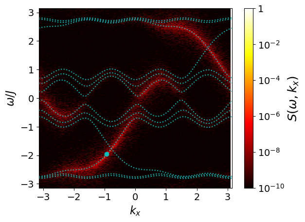
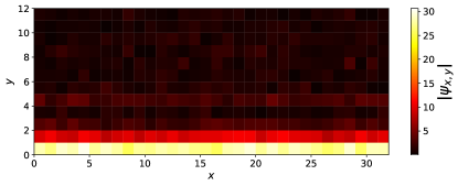
Figure 3: Topological lasing. Lower panel: typical snapshot of the field modulus distribution $|\psi(x,y)|$ at steady-state. Upper panel: wavevector- and energy-resolved spectrum of the field on the $y=1$ edge. The dotted lines are the Harper–Hofstadter bands and the spectral intensities are normalized to the laser emission at $\omega^{las}\simeq-9.774\gamma$, $k_{x}^{las}=-2\pi\frac{19}{128}$. Numerical calculations were performed according to Eq. (20) for a lattice of size $N_{x}=128$, $N_{y}=12$ with periodic boundary conditions along $x$ and a flux density $\alpha=1/4$. System parameters: $J=5\gamma$, $P=2\gamma$, $n_{s}=1000$, $D_{x,y}=\gamma/2(1+\delta_{y,1})$.

With no loss of generality, we focus our attention on the topological bands of a two-dimensional Harper–Hofstadter model. This is a most celebrated topological model and is widely used in studies of topological photonics. By labeling with $x=1,..,N_{x}$ and $y=1,..,N_{y}$ the sites of the two-dimensional lattice, the equations of motion for the field read

$$i\partial_{t}\psi_{x,y}=-J\left[\psi_{x,y+1}+\psi_{x,y-1}+e^{-2\pi i\alpha y}\psi_{x-1,y}+\right.$$

$$\left.+e^{2\pi i\alpha y}\psi_{x+1,y}\right]+\frac{i}{2}\left[\frac{P\delta_{y,1}}{1+n_{x,y}/n_{S}}-\gamma\right]\psi_{x,y}+\sqrt{2D_{x,y}}\xi_{x,y}\ ,$$ (20)

where $\alpha$ is the synthetic magnetic field flux per plaquette in units of the magnetic flux quantum. As in many previous works, we focus on the $\alpha=1/4$ case. To simplify the geometry, we consider a cylindrical lattice with periodic boundary conditions along the $x$ direction, and we introduce the gain medium on all sites of the $y=1$ edge. Inspired by the Wigner approach Gardiner and Zoller (2004), we take the diffusion coefficient to have form $D_{x,y}=(1+\delta_{y,1})\,\gamma/2$. The stronger noise on the edge sites reflects the presence of gain. We have however checked that our results remain qualitatively identical if different spatial distributions of $D_{x,y}$ are used. We have also checked that the statistical results that are going to be discussed in the following of the paper are unchanged if different system geometries are considered, e.g. with open boundary conditions (see e.g. Fig. S3 of sup ).

For the sake of completeness, let us first recall the properties of the underlying Harper–Hofstadter Hamiltonian in the absence of gain, losses and noise. Within the Landau gauge used in Eq. (20), implementing periodic boundary conditions along the $x$ direction makes the system translationally invariant, so that it is convenient to label states by the wavevector $k_{x}$. The dispersion for our $\alpha=1/4$ case is shown by the cyan dotted lines in Fig. 3: it consists of four bands of bulk states delocalized over the whole system, plus two chiral modes localized on each edge and energetically located in the gaps within the bands. On the $y=1$ side per example, the edge state in the lower (upper) gap has positive (negative) group velocity, and viceversa for the other side. The fact that there are no two counter–propagating states on the same edge at the same frequency is at the origin of the topological protection.

We study the temporal evolution of the field according to the stochastic equations (20). Starting the simulation with zero field, noise triggers laser operation by spontaneously breaking the $U(1)$ symmetry. A mean-field study of this physics in the absence of noise with random initial conditions was presented in (Seclì et al., 2019): at steady-state, quasi-monochromatic laser oscillation takes place in a mode which is randomly selected by the initial noise. The probability distribution is peaked at discrete frequencies roughly fixed by the eigenvalues of the underlying finite Harper-Hofstadter model. The distribution is symmetric with respect to zero frequency and has support in the energy gaps of the band structure. The maximum corresponds to the eigenstates that are most localized on the edge for which the effective gain is the strongest: as it was pointed out in (Peano et al., 2016), the $k_{x}$–dependent overlap of the Harper–Hofstadter eigenmode with the gain material determines a non-trivial dependence of the imaginary part of the dispersion.

The main features of the steady-state topological laser operation including noise are illustrated in Fig. 3. In the lower panel we plot a typical example of the field modulus $|\psi_{x,y}|$ for a finite $N_{x}=32,N_{y}=12$ cylindrical lattice, showing localization of the mode on the edge. The upper panel reports instead the power spectral density $S(k_{x},\omega)$ of the field $\psi_{x,1}(t)$ on the $y=1$ edge: the narrow lasing mode is strongly saturated on this scale and is indicated by the cyan circle. Noise-induced fluctuations distribute themselves over all modes but are concentrated on the ones with largest overlap with the $y=1$ side, in particular on the two edge states with opposite chiralities. While the distribution roughly follows the dispersion of the modes in the underlying Harper–Hofstadter model indicated as a cyan dotted line, a complete theory requires a Bogoliubov analysis. This will be the subject of the forthcoming work (Loirette-Pelous, 2019).

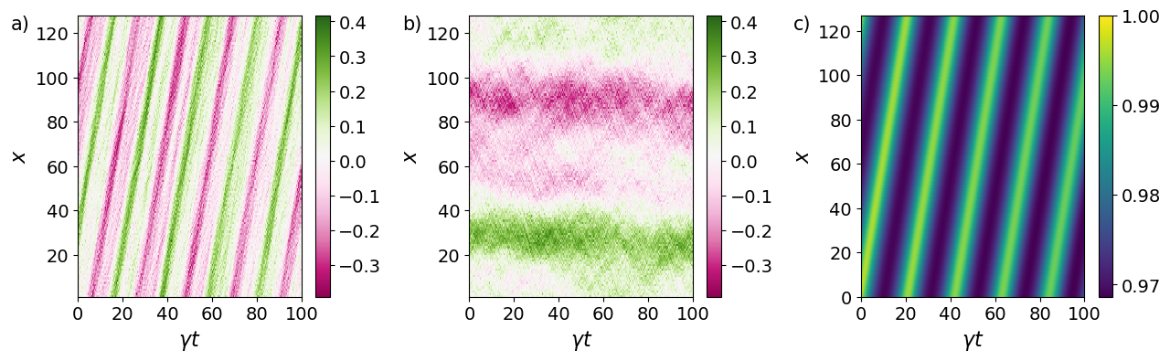
Figure 4: Chiral motion of the phase fluctuations. (a) Spatio-temporal plot of the slowly varying phase of $\psi_{sl}(x,t)$, showing that the fluctuations chirally move around the system. At the steady state in the absence of noise, this plot would be flat. (b) Spatio-temporal plot of the phase of $\psi_{{}_{CM}}(x,t)$ in the co-moving frame: now the fluctuations are observed in their natural frame of reference and evolve slowly. (c) Correlation function $g^{(1)}(x,t)$: since the fluctuations move at $v_{g}$, after a time $t$ the field in $x$ is correlated with the one in $x+v_{g}t$. System parameters: $N_{x}=128,N_{y}=12,J=5\gamma,P=2\gamma,n_{s}=1000,D=2\gamma$.

III.2 Chiral motion of the phase fluctuations

To characterize the spatio-temporal coherence of the emission, we consider the fluctuations of the phase of the one-dimensional field living on the amplifying boundary of the Harper–Hofstadter lattice, $\psi(x,t)\equiv\psi_{x,1}(t)$.

In the steady-state of laser operation, the phase displays slow fluctuations around a carrier wavevector $k_{x}^{las}$ and frequency $\omega^{las}$: the former can be extracted from the (spatial) winding number of the phase around the system, the latter can be determined by fitting the evolution of the field phase on single sites. In the spectrum of Fig.3, they are indicated by the position of the cyan circle. While a precise determination of these quantities can be important from the applicative point of view, they are somehow uninteresting from the statistical mechanics point of view, since they are mostly determined by the deterministic dynamics of the device and are weakly affected by the fluctuations.

In order to remove the carrier frequency and wavevector and concentrate on the stochastic fluctuations, we define the slowly varying field

$${\psi}_{sl}(x,t)\equiv e^{-i(k_{x}^{las}x-\omega^{las}t)}\,\psi(x,t).$$ (21)

Looking at the phase of a typical realization of $\psi_{sl}(x,t)$ shown in Fig. 4(a), we easily recognize a phase fluctuation pattern that moves at a constant velocity and gets slowly distorted. The drift velocity can be inferred from the dispersion $\omega_{em}(k_{x})$ of the lasing chiral edge mode, which has group velocity $v_{g}=\frac{d\omega_{em}}{dk_{x}}(k_{x}^{las})$ and curvature $J_{eff}(k_{x}^{las})=\frac{1}{2}\frac{d^{2}\omega_{em}}{dk^{2}_{x}}(k_{x}^{las})<J$.

In order to focus on the intrinsic dynamics of the phase fluctuations, we plot in Fig. 4(c) a typical realization of the phase evolution seen from the moving frame at $v_{g}$,

$$\psi_{{CM}}(x,t)\equiv\psi_{sl}(x+v_{g}t,t).$$ (22)

For the relatively strong inter-site coupling $J=5\gamma$ and relatively small system size $N_{x}=128$, the phase fluctuations develop very slowly and remain quite small. Their magnitude gets larger if the mean intensity $n_{0}$ is reduced, the inter-site coupling $J$ is reduced, or larger systems are considered. This will be discussed in Sec.III.4.

While the transformation to $\psi_{{}_{CM}}(x,t)$ allows for a direct visualization of the phase dynamics, it is also possible to study the fluctuations circulating along the edge by computing the space–time correlation function of the original field,

$$g^{(1)}(x,t)=|\langle\psi^{*}(x,t)\psi(0,0)\rangle|,$$ (23)

where the average is taken over the noise and invariance under temporal $t$ and spatial $x$ translations is assumed. This analysis requires no preliminary estimate of $k_{x}^{las}$ and $\omega^{las}$ and will be our workhorse in the next sections. As it is apparent looking at the smooth stripes in Fig. 4(c), the analysis of $g^{(1)}(x,t)$ is the cleanest way to extract the velocity at which fluctuations travel. The result $v_{g}\simeq 6.07\,\gamma a$ is perfectly compatible with the group velocity $v_{g}\simeq 6.08\,\gamma a$ obtained from the linear dispersion of the chiral edge mode (see also Fig. S4 of sup ).

III.3 Correlated side-peaks in the emission spectrum

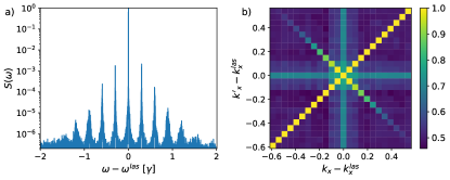
Figure 5: Correlated side-peaks in the emission spectrum. (a) Spectrum of the field on a single resonator located on the amplified edge. The spacing of the side–peaks is determined by the quantization of the wavevector $k_{x}$ around the periodic direction. The side–peaks are generated by parametric scattering processes from the lasing mode into pairs of symmetrically located modes. (b) Color plot of the momentum-space correlation function (25) in the $k_{x},k_{x}^{\prime}$ plane showing -among other- strong correlations between symmetrically located modes.

A complete understanding of the spectral distribution $|\psi(k_{x},\omega)|^{2}$ obtained by spatio-temporal Fourier transform and shown in Fig. 3(b) requires inspecting the Bogoliubov modes on top of the noiseless lasing state. This will be the subject of a forthcoming work (Loirette-Pelous, 2019).

For the moment, we restrict our discussion to a few simple yet important remarks on the emission spectrum from each site. In Fig. 5(a) we show the emission spectrum defined as

$$S(\omega)=\frac{1}{N_{x}}\sum_{x}|\psi(x,\omega)|^{2}$$ (24)

for the parameters and lasing point shown in Fig. 3(b). In addition to the main lasing peak, the emission spectrum displays a comb-like structure with a series of symmetric side-peaks: the frequency spacing is determined by the quantization of the momentum along the periodic direction and is approximatively $v_{g}\frac{2\pi}{N_{x}}$.

The visibility of the comb is not merely due to the existence of eigenstates at those specific values of the frequency, but their population by noise is enhanced by correlations. This is illustrated in Fig. 5(b) where we show the normalized momentum–space intensity–intensity correlation function

$$R^{(2)}(k_{x},k^{\prime}_{x})=\frac{\langle n_{k_{x}}n_{k^{\prime}_{x}}\rangle}{\sqrt{\langle n_{k_{x}}^{2}\rangle\langle n_{k^{\prime}_{x}}^{2}\rangle}}.$$ (25)

Here, the momentum–space densities $n_{k_{x}}$ are evaluated at the same time over the whole edge, $n_{k_{x}}(t)=|\psi(k_{x},t)|^{2}$.

Several features are visible in this plot. The diagonal line for $k_{x}=k_{x}^{\prime}$ is due to a trivial self-correlation and $R^{(2)}$ is here equal to $1$. For generic pairs of modes, the fact that $g^{(2)}(k_{x})=2$ for $k_{x}\neq k_{x}^{las}$ implies that the background value is $R^{(2)}=0.5$. When one (two) modes coincide with the lasing one, $R^{(2)}$ is equal to $1/\sqrt{2}$ (1), which explains the vertical and horizontal stripes and the central peak. The most interesting feature is the stripe on the anti-diagonal, corresponding to correlations between symmetrically located modes such that $k_{x}+k_{x}^{\prime}=2k_{x}^{las}$. For the first two pairs of side–peaks, this correlation is nearly perfect, indicating that these modes are populated in pairs by parametric scattering processes.

Such correlations are of course not specific of topological systems but can be observed also in the trivial systems studied in the previous Sec. II, albeit with a suppressed intensity due to the curvature of the dispersion. In analogy to exciton-polariton systems pumped around the magic angle Carusotto and Ciuti (2013), the magnitude of these parametric correlations would be reinforced again if lasing was made to operate around the inflection point of the dispersion.

III.4 KPZ spatio-temporal correlations

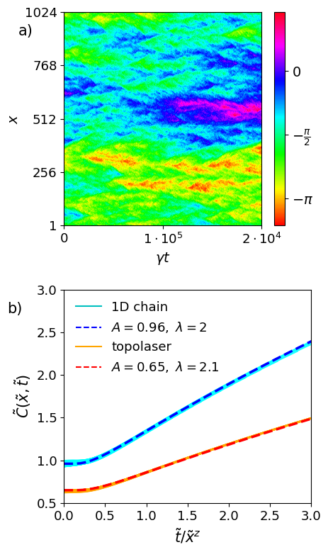
Figure 6: KPZ dynamics of topological lasing. (a) Typical example of the space-time dynamics of the phase of the field $\psi_{{}_{CM}}(x,t)$ on the system edge seen from the comoving frame. (b) Correlators $\tilde{C}(\tilde{t},\tilde{x}^{z})$ for $x=\pm 30,...,\pm 160$ (small lines) for the topological device lasing into the $k_{x}=-2\pi\frac{155}{1024}$ mode (orange) and for the non-topological one-dimensional array lasing in the $k_{x}=0$ mode (cyan). Red and blue dashed lines indicate the KPZ universal function (31) on which all curves collapse. System parameters: $N_{x}=1024$, $J=0.5\gamma$, $P=2\gamma$, $n_{S}=1000$, $D_{x,y}=\gamma/2(1+\delta_{y,1})$.

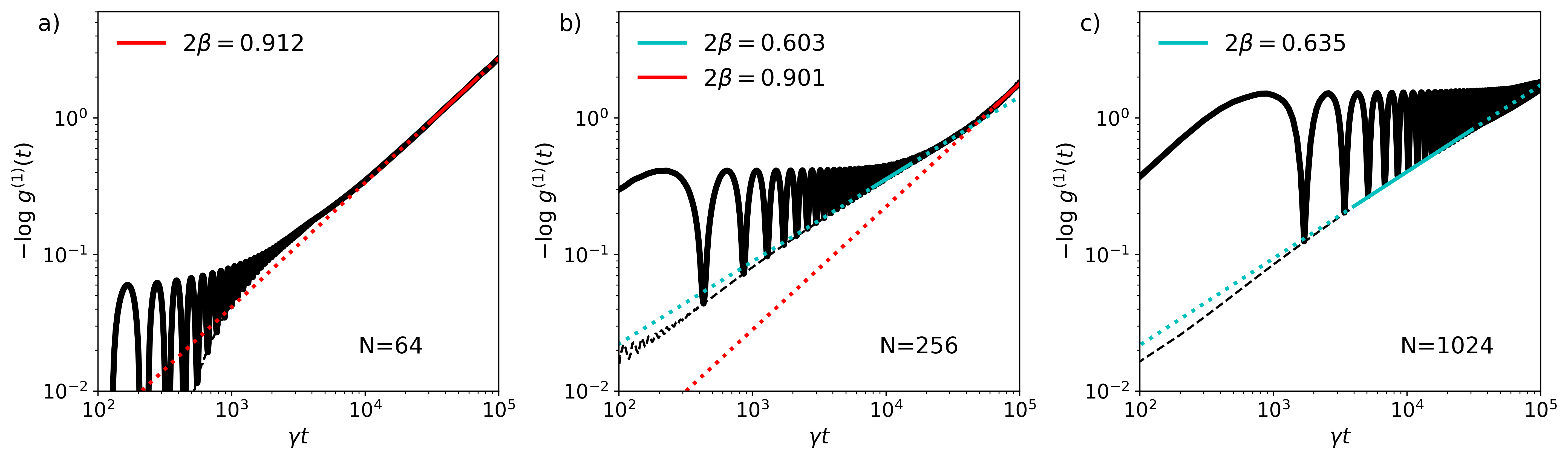
Figure 7: Kardar-Parisi-Zhang to Schawlow-Townes crossover in a finite–size topological laser. This plot is the analogous of Fig. 1 for the topological laser. The thick black lines correspond to the logarithm of the temporal correlation for a given site on the edge of the lattice. The thin dashed lines show the temporal evolution of the coherence $-\log g_{{}_{CM}}^{(1)}(t)$ seen from the reference frame comoving with the edge state. For increasing system sizes and a given temporal window, a crossover between an exponential (red fits) and a KPZ (cyan fits) decay of the coherence is observed. The amplitude of the oscillations is inversely proportional to the spatial coherence of the device. In the long-time limit, only the global phase matters and the oscillations fade away.

The discussion of the emission spectrum presented in the previous subsection gives first hints of the complexity of the multi-mode dynamics of fluctuation dynamics. Here we will build a complete theoretical picture of the spatio-temporal coherence of the topological laser.

To get a first hint on the behaviour, we can make the assumption that the field on the edge can be described in the comoving frame by the 1D equation

$$i\partial_{t}\psi_{{}_{CM}}(x,t)=(-J_{eff}+i\eta)\nabla^{2}\psi_{{}_{CM}}+\\ +\frac{i}{2}\left[\frac{P_{eff}}{1+n_{S}|\psi_{{}_{CM}}|^{2}}-\gamma\right]\psi_{{}_{CM}}+\sqrt{2D}\,\xi.$$ (26)

Here $J_{eff}$ is given by the curvature of the bare Harper–Hofstadter topological mode, $P_{eff}$ is chosen as to retrieve the numerical mean intensity $n_{0}$ on the edge, and $\eta$ accounts phenomenologically for the $k$-dependent localization of the lasing mode on the edge of the lattice. A rigorous account of this dimensional reduction procedure will be presented in (Loirette-Pelous, 2019).

Assuming a fast relaxation of the intensity fluctuations, we can then restrict our attention to the dynamics of the phase. By neglecting terms containing four derivatives (both the linear, Galilean-preserving ones and the nonlinear, Galilean-breaking ones as shown in Sec. SI sup ), one gets to a motion equation for the phase of the KPZ form:

$$\partial_{t}\phi=\eta\nabla^{2}\phi+J_{eff}(\nabla\phi)^{2}+\sqrt{\frac{D}{n_{0}}}\xi.$$ (27)

Since $\eta$ is the less controlled parameter of the model, we do not perform the usual KPZ rescaling (He et al., 2015) to yield an equation containing the effective nonlinearity as the only one parameter. Rather, we rely on the rescaling Eqs. (9) with the effective parameters $J\to J_{eff},P\to P_{eff}$; this transformation does not depend on $\eta$ and yields

$$\partial_{\tilde{t}}\tilde{\phi}=\frac{\eta t_{*}}{l_{*}^{2}}\tilde{\nabla}^{2}\tilde{\phi}+(\tilde{\nabla}\tilde{\phi})^{2}+\xi.$$ (28)

In these units we then expect the KPZ nonlinearity to be close to $\lambda=2$; this value is also protected from renormalization induced by the quartic derivative term in the KSE (Ueno et al., 2005). It is thus natural to expect that the coherence of the topological laser will closely resemble the one of the generic extended laser discussed in Sec.II. In what follow, we proceed to numerically verify this statement on simulations of the stochastic laser equations in the topological two-dimensional lattice.

Based on our previous discussion, we expect that the KPZ universal dynamics occurs, in a lattice of $N_{x}$ sites, on timescales shorter than the saturation time $\sim N_{x}^{z}$ (after which the Schawlow–Townes like behavior described above sets in) but larger than the timescales where the linear Bogoliubov dynamics and non–universal effects dominate. Having a sizable window where to observe KPZ physics then requires the system to be large enough, precisely it should be at least $N_{x}a\gg\sqrt{2}\pi l^{*}$ (Gladilin et al., 2014). We thus consider a large system of length $N_{x}=1024$ with periodic boundary conditions along $x$ and with $N_{y}=12$ points along the open direction $y$. In order to clearly observe KPZ physics while keeping intensity fluctuations within 15% and having a tractable system size, it is beneficial to use a small inter-site coupling $J=0.5\gamma$.

One may argue that such a value of the coupling $J$ (and thus of the topological gap) is comparable with the bare linewidth $\gamma$. Such narrow topological gaps are very relevant for experimental implementationsBahari et al. (2017), but it is not a priori obvious whether in this regime the chiral edge modes survive losses. While this is indeed a serious issue to observe chiral edge propagation in passive systems, it is a crucial result of laser theory that the laser linewidth above threshold can be orders of magnitude smaller than $\gamma$. Our numerical simulations confirm stable lasing into the chiral edge mode even for for small $J/\gamma$; in particular, the robustness of topological lasing has been verified in the presence of a strong defect on the edge, as reported in Fig. S5 sup .

To numerically highlight the KPZ physics we have performed 20 simulations of the full two-dimensional lattice of duration $\gamma T=5\cdot 10^{5}$, starting from a plane wave with the wavevector value for which the Harper–Hofstadter eigenstate is most localized on $y=1$, that is $k_{x}=-2\pi\frac{155}{1024}$. For each run the correlation function $\langle\psi^{*}(x,t)\psi(0,0)\rangle$ on the edge site is computed and then averaged over the 20 trials to yield $g^{(1)}(x,t)$. The typical dynamics occurring in a time $\gamma T=2\cdot 10^{4}$ is depicted in Fig. 6(a), where the phase of the field $\psi_{{}_{CM}}(x,t)$ along the edge is shown in the comoving frame: a structure similar to the fractal structure of interface growth can be recognized.

Defining the correlation function in the comoving frame as

$$g_{{}_{CM}}^{(1)}(x,t)=|\langle\psi_{{}_{CM}}^{*}(x,t)\psi_{{}_{CM}}(0,0)\rangle|$$ (29)

and the rescaled correlator as

$$\tilde{C}(\tilde{t},\tilde{x}^{z})\equiv-2(\phi^{*})^{-2}\tilde{x}^{-2\chi}\log g_{{}_{CM}}^{(1)}(\tilde{x},\tilde{t}),$$ (30)

KPZ universality requires that

$$\tilde{C}(\tilde{x},\tilde{t})=\tilde{C}(\tilde{t}/\tilde{x}^{z})=\left(\frac{1}{2}\lambda A^{2}s\right)^{2/3}g_{KPZ}\left(\frac{1}{(2\lambda^{2}As^{2})^{1/3}}\right)$$ (31)

with $s=\tilde{t}/\tilde{x}^{z}$ and $z=3/2$ on the right-hand side and $g_{KPZ}$ a universal function discussed in Sec.II.2. In particular, one has $\tilde{C}(0)=A$.

In Fig.6(b) we plot $\tilde{C}(\tilde{x},\tilde{t})$ for $x=\pm 30,...,\pm 160$ and demonstrate that within an excellent approximation they only depend on $\tilde{t}/\tilde{x}^{z}$ (to correct for the finite size effects, we actually plot $\tilde{C}(\tilde{x},\tilde{t})/(1-|x|/N_{x})$, as illustrated in Fig. S6 (sup, )). The orange and cyan series correspond to calculations for respectively the topological laser and the trivial one-dimensional chain laser in the $k=0$ mode discussed in Sec.II.2. The same physical parameters have been used in both cases.

The crucial point about Fig.6(b) is that the phase, the space and the time have been rescaled by the $\phi^{*}$, $l^{*}$, $t^{*}$ values obtained by using the effective masses and gain parameters: for the topological laser, $J_{eff}$ is the curvature of the Harper–Hofstadter band at the lasing point and $P_{eff}$ is chosen in order to reproduce the observed intensity on the edge. For instance, $J_{eff}\simeq 0.319\gamma$ hence $l^{*}\simeq 1.92$ here. A detailed report of possible mappings of the $2D$ topological laser to a $1D$ one will be presented soon(Loirette-Pelous, 2019).

As anticipated, the Renormalization Group analysis (Ueno et al., 2005) predicts for the $1D$ array lasing in the $k^{las}=0$ mode that the rescaled KSE Eq. (11) flows to the low energy effective KPZ theory Eq. (10) with $\lambda=2$, since, thanks to the Galilean invariance holding for KSE and KPZ equations, the nonlinear coupling is not renormalized. Indeed, in this case the rescaled correlation functions collapse to a unique curve as shown in Fig.6(b) and this curve is excellently fitted (blue dashed line) using (31) with $\lambda=2$ and $A=0.96$, as expected from the Galilean invariance argument. For the topological laser, the curves again collapse onto a single curve, which is well fitted using $\lambda=2.1$ and $A=0.65$ (red dashed line). The value $\lambda=2.3$ with $A=0.63$ is an upper bound for the fitted value of the nonlinearity.

Notice that for the topological laser there is no a priori guarantee that a Galilean invariant KSE holds microscopically; on the contrary, an analysis on the lines of (Gladilin et al., 2014; Altman et al., 2015) suggests that a rescaling with $J_{eff}$ still yields a microscopic $\lambda=2$, but other terms should also be added in Eq. (10), e.g. of the kind $\nabla^{2}\phi(\nabla\phi)^{2}$, $(\nabla^{2}\phi)^{2}$, $\nabla^{3}\phi\nabla\phi$, etc. These additional terms come from effective imaginary derivatives due to the $k_{x}$ dependent localization of the Harper–Hofstadter eigenstates on the edge; in particular, they break Galilean invariance and one may expect that they significantly renormalize the effective KPZ parameters, since they contain the same number (four) of derivatives as the KSE term. From the numerics, it turns out that the renormalization of $\lambda$ is instead small.

Still, it is interesting to note that the curves for the topological laser (in the properly rescaled units) sit below the ones of the trivial one-dimensional laser array. This feature can be traced back to the imaginary term proportional to $\eta$ in (26) that accounts for the $k$-dependence of the edge mode penetration in the bulk. This term stabilizes the emission and makes the topological device more coherent than the 1D laser with the corresponding $J_{eff},P_{eff}$. The “ultraslow decay of fluctuations” that was observed in (Seclì et al., 2019) is indeed a consequence of the Goldstone branch and thus is a general feature of spatially extended lasers. The crucial role of $\eta$ in topological devices is apparent already at the level of Bogoliubov analysis (Loirette-Pelous, 2019), at least for class-A lasers. It is also remarkable that the very noisy field in the bulk that is visible e.g. Fig. S2 of sup does not impact the coherence of the edge mode.

We conclude this section with a brief remark on the experimental protocol to assess KPZ physics. The analysis of the correlation functions $g_{{}_{CM}}^{(1)}(x,t)$ shown in Fig.6.b was carried out in the reference frame comoving with the chiral mode, while in the lab one can easily measure correlation functions between different points at different times $g^{(1)}(x,t)$. However, since the two correlations functions are simply related by $g_{{}_{CM}}^{(1)}(x,t)=g^{(1)}(x-v_{g}t,t)$, the interesting $g_{{}_{CM}}^{(1)}$ can be extracted by a straightforward post-processing of $g^{(1)}(x,t)$. Graphically, this amounts to tilt the correlation function of Fig. 4(c) with the suitable $v_{g}$ so to have the maximum of $g^{(1)}(x,t)$ at $x=0$ for all times $t$ (see Fig. S4 sup ).

III.5 Temporal coherence and linewidth

After having confirmed that the long-time, large-distance spatio-temporal coherence of the topological laser is well described by the KPZ model, we now proceed to investigate the problem of the coherence time of a realistic, finite-size device. Rather than analyzing with high resolution the linewidth of the main spectral peak of Fig. 5(a), we work in real time and, with a concrete optical experiment in mind, we monitor the temporal coherence of the emission from a given site.

III.5.1 KPZ to Schawlow-Townes crossover

As compared to our discussion of the trivial case in Sec.II.2, there is the complication that phase fluctuations undergo a chiral motion around the system, so the coherence function of a given site displays the strong temporal oscillations visible in Fig. 4(c).

As a first step, we illustrate the crossover between KPZ coherence decay and Schawlow–Townes for different system sizes $N_{x}$. In Fig. 7 we show the temporal evolution of the phase diffusion $-\log g^{(1)}(t)$ (thick solid black lines) and $-\log g_{{}_{CM}}^{(1)}(t)\equiv-\log g_{{}_{CM}}^{(1)}(0,t)$ (thin dashed black lines) in a given temporal window for increasing $N_{x}=64,256,1024$. As expected, these curves show sharp local minima of $-\log g^{(1)}(t)$ corresponding to local maxima of the coherence. As they originate from chiral motion of fluctuations around the system, these oscillations have a period $N_{x}/v_{g}$. The value of the coherence at these minima provides a discrete sampling of the equal-space coherence function $g_{{}_{CM}}^{(1)}(t)$. Similarly, the local maxima (minima of coherence) provide a sampling of $g_{{}_{CM}}^{(1)}(N_{x}/2,t)$.

Looking at the envelope of the minima for the largest system, we see that the agreement of Fig. 7(c) with the KPZ result is very good. In particular, it makes a clear distinction from the predictions of the linear Edwards–Wilkinson model for which the exponent would be different. Note also that the oscillations in $-\log g^{(1)}(t)$ are well visible at short times but fade away at long times, where only the global phase of the field over the whole lattice matters and no oscillation is any longer visible. For the same reason, monitoring a resonator not on the edge one sees a fast initial decay, but at long times the phase diffusion is the same as the edge, as sketched in Fig. S2 (sup, ).

For the smaller systems, the different functional form shown in Fig.7(a) displays an exponential decay of the late-time coherence. As one can see comparing with panel (b), the late-time exponential decay is always there, it is just pushed to extremely long times in the largest systems. This is in close analogy with what we had found in Sec.II.3 for the trivial system.

III.5.2 Linearized Bogoliubov prediction for the linewidth

The natural question is now to estimate the rate of this exponential decay and see how it scales with the size of the system. As a first step, we adopt a linearized Bogoliubov approach. For generic systems of $N$ sites (labelled as $\vec{x}$) of arbitrary dimensionality, let us call $\mathcal{L}_{las}$ the $2N\times 2N$ Bogoliubov matrix of the linearized dynamics on top of the lasing steady-state. Let $V=\{V_{\vec{x}\sigma,p}\}$ be the invertible matrix which diagonalizes $\mathcal{L}_{las}$, where the pseudo-spin $\sigma=\uparrow,\downarrow$ indicates the particle and hole components of the Bogoliubov problem and $p$ labels the $2N$ eigenmodes. The Goldstone mode $V_{\vec{x}\sigma,G}$, that we assume to be unique with all other excitations having a finite life-time, is the eigenstate with zero eigenvalue. As usual, its spatial shape follows the one of the lasing mode. The effective noise acting on the lasing mode will be determined by the projection of the bare noise on it. For generality we consider a position dependent bare noise $D_{\vec{x}}$. Then, in the Bogoliubov approximation, the phase drift associated with the Goldstone mode is given by

$$\langle\Delta_{t}\phi^{2}\rangle=\Phi_{G}^{2}\sum_{\vec{x}}D_{\vec{x}}\ (V^{-1})_{G,\vec{x}\uparrow}(V^{-1})_{G,\vec{x}\downarrow}\ |t|$$ (32)

where the summation represents the projection of the noise on the Goldstone mode and

$$\Phi_{G}=\Phi_{G}(\vec{x})=\frac{-i}{n_{0}(\vec{x})}\left[\psi^{*}_{0}(\vec{x})V_{\vec{x}\uparrow,G}-\psi_{0}(\vec{x})V_{\vec{x}\downarrow,G}\right]$$ (33)

is actually independent of $\vec{x}$ and provides the normalization of the Goldstone mode phase component.

If $VV^{\dagger}=1$ a very clear expression holds for the Schawlow–Townes line:

$$\gamma_{ST}=\frac{\sum_{\vec{x}}D_{\vec{x}}n_{\vec{x}}}{n^{2}_{tot}}=\frac{D_{n}}{n_{tot}}$$ (34)

with $n_{tot}=\sum_{\vec{x}}n_{\vec{x}}$ and $D_{n}=\sum_{\vec{x}}D_{\vec{x}}n_{\vec{x}}/\sum_{\vec{x}}n_{\vec{x}}$. This is for instance the case of a spatially uniform, topologically trivial system, for which the different wavevectors decouple and the sector of $\mathcal{L}_{las}$ at the lasing wavevector $\vec{k}_{las}$ is diagonalized by a $2\times 2$ unitary matrix $VV^{\dagger}=1$, since modulus and phase are decoupled for the lasing mode.

The situation is a bit more complicated in the topological case: the $k_{x}=0$ sector has dimension $2N_{y}\times 2N_{y}$ and $V$ is not unitary $VV^{\dagger}\neq 1$, so the theory discussed above does not hold. However, for the considered parameters it turns out that $VV^{\dagger}\simeq 1$, so the approximate expression

$$\tau_{ST}=\frac{2}{\gamma_{ST}}\simeq 2\frac{\left[\sum_{x,y}n_{x,y}\right]^{2}}{\sum_{x,y}n_{x,y}D_{x,y}}=2N_{x}\frac{\sum_{y}n_{1,y}}{D_{n}}.$$ (35)

is expected to provide an accurate approximation. In the standard laser theory the non–orthogonality of $V$ is also known under the terminology of Petermann factor and excess noise Siegman (1989a, b). The transverse Petermann factor, defined here as the ratio $\mathcal{K}=\frac{\gamma_{ST}}{D_{n}/n_{tot}}$, for the topological laser device is around $\mathcal{K}\simeq 1.002$ for $J=5\gamma$ and $\mathcal{K}\simeq 1.1$ for $J=0.5\gamma$ (the difference to be attributed to gain guiding), meaning that, within the linearized Bogoliubov approximation, the laser emission is for all practical purposes determined only by the total number of photons in the device, which is the textbook, optimal case.

III.5.3 Numerical results for the linewidth

In order to assess the validity range of the Bogoliubov calculation, numerical simulations of the stochastic equations have been performed for the full two-dimensional model. The numerical predictions for the coherence time of the topological laser are shown by the red and orange triangles in Fig. 2 as a function of the system size. The dashed line shows the theoretical prediction Eq. (32). From these results, one concludes that the topological laser behaves again similarly to the topologically trivial one-dimensional laser array: for small $N_{x}$ the agreement with the Bogoliubov-Schawlow-Townes model of phase diffusion is excellent and the coherence grows proportionally to $N_{x}$. On the other hand, marked deviation occur for larger systems with a slower-growing coherence time. (Notice that the dependence of the Petermann factor on $N_{x}$ is negligible and via $k_{x}^{las}$.)

To conclude our discussion, it is interesting to note that the Bogoliubov-Schawlow–Townes prediction that well captures the emission linewidth for small systems does not depend on $J_{eff}$ nor on the dispersion of the Bogoliubov modes at $k_{x}\neq 0$. On the other hand, the deviation observed for larger systems does strongly depend on $J_{eff}$, which pinpoints the crucial role of the KPZ nonlinearities illustrated above .

IV Lasing with on–site disorder

The general message of the previous Section was that the coherence properties of a topological laser follow the same KPZ dynamics as the ones of a topologically trivial, one-dimensional laser array. This conclusion is not restricted to the well-known KPZ features in the infinite system limit, but also applies to the dependence of the coherence time on the system size and to the marked deviations from the single-mode Schawlow-Townes prediction.

In this Section we investigate the effect of static disorder on the coherence of the laser emission. A certain degree of fabrication imperfections and inhomogeneities is in fact expected to be always present in realistic devices. Our numerical study points out a dramatically different behaviour of topologically trivial vs. topological systems: disorder has a strong impact on the coherence of a topologically trivial system, a small amount of disorder being able to give a wide range of realization-dependent, chaotic and multi-mode phenomena. On the other hand, the temporal coherence of a topological laser is robust against a sizable disorder and emission remains well monochromatic as long as the disorder magnitude is not so large to close the topological gap.

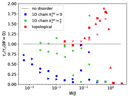
Figure 8: Topological robustness of the temporal coherence. Plot of the coherence time (normalized to the clean system value) as a function of the strength $W$ of the disorder. Different markers refer to different realizations of disorder. Blue and green markers are for a non-topological one-dimensional laser array lasing at $k^{las}=0$ (blue) or $k^{las}=\frac{\pi}{5}$ (green). Red markers are for the topological laser with periodic boundary conditions (squares and triangles) and with open boundary conditions (crosses). Same marker shapes correspond to the same spatial distribution of the disorder potential except for the overall strength $W$.

IV.1 Lasing in a non-topological one-dimensional array with disorder

We start by considering the effect of on–site disorder on the lasing properties of a non-topological array of resonators. We do not aim here to a general discussion of the theory of lasing in disordered systems or to make a connection with random lasers (Wiersma, 2008), but our purpose is just to provide a benchmark to assess the features of a topological laser.

Along all this section, a disordered potential is added to Eqs. (7) and (20) in the form,

$$i\partial_{t}\psi_{\vec{x}}=\ldots+W\mathcal{G}(0,1)\psi_{\vec{x}},$$ (36)

where $\mathcal{G}(0,1)$ is a Gaussian random variable with mean 0 and variance 1. For the sake of definiteness, we restrict here to the $N_{x}=128$ and $J=5\gamma$ case. The lasing dynamics in the presence of disorder is in general very complex, but, since our ultimate goal is a qualitative comparison with the topological laser, we focus here on the coherence time of the system for various values of disorder $W$, and in particular on looking whether there is a clear threshold value of disorder above which coherence collapses.

For linear waves, the sensitivity of the eigenstates at a given energy to a static perturbation is proportional to the spectral density of states. Then, in order to have a fair comparison of the trivial and topological cases, we consider lasing both at $k^{las}=0$ and at $k^{las}=\frac{\pi}{5}$. This latter case has a finite group velocity (and hence a density of states) comparable to the one of the chiral edge mode of the Harper–Hofstadter model in its central part and for these reasons it seems the most natural way of benchmarking the topological laser.

In Fig. 8, we plot the coherence time normalized to the value in the absence of disorder. In particular, we use an exponential fit to extract the coherence time $\tau_{c}$ for each site (an exponential fit is used even if the shape of $g^{(1)}(t)$ is in general very complex) and we plot the average over the lattice. Markers with the same shape indicate that the same realization of disorder and the same initial conditions have been used, while only the overall strength factor $W$ is varied.

From the plot, we see that already a very small disorder has a marked impact on the coherence time of the device, the threshold value depending on $k_{x}^{las}$. While a detailed description of all possible behaviours depending on the disorder realization goes beyond the scope of this work (some illustrative examples are shown in the SI sup ) and not fully understood non-monotonic behaviours are observed in some cases, we can safely conclude that the coherence is quickly lost in most of the realizations. For strong disorder $W\sim 0.8\gamma$ laser operation gets fragmented and different portions of the sample end up lasing at different frequencies (see Fig. S7 of sup ).

IV.2 Lasing in a topological disordered system

The same protocol was repeated for the topological laser on a $N_{x}=128$ times $N_{y}=12$ stripe with periodic boundary conditions and $J=5\gamma$. The results are reported in red squares and triangles in Fig. 8. Simulations were also performed with fully open boundary conditions and gain distributed along the whole edge, yielding the same conclusions. The system size with $N_{x}=52$ and $N_{y}=14$ was chosen to have an edge with the same length of 128 sites. The results are shown in the figure by the red $\times$ markers.

In contrast to the non-topological case, the behavior of the topological laser remains quite regular when disorder is introduced and different realizations show very similar features. Temporal and spatial coherence is very well preserved (as apparent in Fig. S8 (sup, )) until a marked threshold at a value of disorder $W_{thr}\sim J$ on the order of the topological gap of the underlying Harper–Hofstadter model. Beyond this value, spatial and temporal coherence are rapidly lost.

More precisely, for small $W$, disorder has a minor impact at all and the laser field in the chiral edge mode is able to continuously travel around the system. For intermediate values of the disorder strength, but still below the threshold, there is a surprising and systematic enhancement of the temporal coherence. The coherence time remains anyway well below than the ultimate Bogoliubov–Schawlow–Townes bound (32) which for our parameters and $W=0$ is $\tau_{ST}/\tau_{c}\simeq 2.7$. A tentative interpretation of these observations is that disorder partially hampers the KPZ nonlinear dynamics that is responsible for the deviation from the linear Bogoliubov-Schawlow-Townes curve in Fig. 2.

Finally, it is worth noting that in the previous paragraph we initialized the non-topological laser operation in either the $k^{las}=0$ or the $k^{las}=\frac{\pi}{5}$ modes, finding quantitative different behaviours. In the topological case, instead, the vacuum of the field can be taken as the initial condition with no noticeable change, demonstrating that disorder does not affect the capability of the topological laser to autonomously reach its coherent steady state.

V Conclusions

In this work we have investigated the spatio-temporal coherence properties of arrays of coupled laser resonators, focusing on analogies and differences between a non-topological one-dimensional chain and chiral edge-state lasing in a 2D topological Harper–Hofstadter lattice.

In the non-topological case we have highlighted the crossover for growing observation times from a Kardar-Parisi-Zhang scaling to a Schawlow-Townes-like phase-diffusion regime. Also, for a growing system size the long-time phase diffusion rate displays a crossover from the standard single-mode Schawlow-Townes linewidth to a faster decoherence determined by the nonlinear and multi-mode dynamics of spatial fluctuations. Provided one reasons in the reference frame moving at the group velocity of the chiral mode, these results are found to directly apply to the chiral laser emission in the edge states of a topological laser device. In particular, in the Schawlow-Townes regime the topological laser emission is characterized by a transverse Petermann factor very close to one: this further clarifies the nature of the topological localization on the edge, proving that the coherence is not affected by the geometry of the cavity, as it instead occurs for lasing in open resonators. For all practical purposes the coherence time is then determined by the total number of photons in the device, which is the optimal scenario.

While for clean samples the spatio-temporal correlations behave very similarly for the topological and trivial devices, topological protection entails a much larger resilience to inhomogeneities. For the non-topological one-dimensional chain, static disorder is in fact able to spatially localize the lasing mode and/or break it into several disconnected and incoherent pieces. On the other hand, the chiral motion of the edge state of a topological laser device is able to maintain the spatial and temporal coherence across the whole sample up to much larger values of the disorder strength of the order of the topological gap. These results open exciting perspectives both for technological applications and for studies of fundamental physics using topological lasers.

From the theoretical point of view, ongoing research includes the classification of the different Kardar-Parisi-Zhang universality subclasses for our model (Squizzato et al., 2018), the extension of our study to class-B semiconductor lasers by explicitly including the carrier dynamics (Longhi et al., 2018) and different kinds of optical nonlinearities that may lead to further decoherence processes. On a longer run, a natural step involves the generalization of the topological laser concept to photonic lattices with different dimensionalities and different band topologies (Ozawa et al., 2019).

From the experimental side, the effectively periodic boundary conditions naturally enjoyed by a chiral edge mode are extremely promising to suppress undesired spatial inhomogeneities and boundary effects in experimental studies Baboux (2019) of the critical properties of different non-equilibrium statistical models.

On the application side, we demonstrated a level of coherence quantitatively comparable or even better than the corresponding non-topological device, with the crucial advantage that the coherence of a topological laser is robust against the presence of static disorder. While a related robustness result was established in Harari et al. (2018) for the slope efficiency of the laser device, our crucial result is that it also applies to the coherence properties. This confirms the strong promise that topological laser hold for practical opto-electronic applications.

References

- Siegman (1987) A. E. Siegman, Lasers (Oxford University Press, 1987).
- Svelto (2010) O. Svelto, Principles of Lasers (Springer US, 2010).
- Haken (1983) H. Haken, Synergetics (Springer Berlin Heidelberg, 1983).
- Gardiner and Zoller (2004) C. Gardiner and P. Zoller, Quantum noise: a handbook of Markovian and non-Markovian quantum stochastic methods with applications to quantum optics, Vol. 56 (Springer Science & Business Media, 2004).
- Chiocchetta et al. (2017) A. Chiocchetta, A. Gambassi, and I. Carusotto, “Laser operation and bose–einstein condensation: Analogies and differences,” in Universal Themes of Bose–Einstein Condensation, edited by N. P. Proukakis, D. W. Snoke, and P. B. Littlewood (Cambridge University Press, 2017) pp. 409–423.
- Keeling et al. (2017) J. Keeling, L. M. Sieberer, E. Altman, L. Chen, S. Diehl, and J. Toner, “Superfluidity and phase correlations of driven dissipative condensates,” in Universal Themes of Bose–Einstein Condensation, edited by N. P. Proukakis, D. W. Snoke, and P. B. Littlewood (Cambridge University Press, 2017) pp. 205–230.
- Ozawa et al. (2019) T. Ozawa, H. M. Price, A. Amo, N. Goldman, M. Hafezi, L. Lu, M. C. Rechtsman, D. Schuster, J. Simon, O. Zilberberg, and I. Carusotto, Rev. Mod. Phys. 91, 015006 (2019).
- Haldane and Raghu (2008) F. D. M. Haldane and S. Raghu, Phys. Rev. Lett. 100, 013904 (2008).
- Wang et al. (2009) Z. Wang, Y. Chong, J. D. Joannopoulos, and M. Soljačić, Nature 461, 772 (2009).
- Smirnova et al. (2019) D. Smirnova, D. Leykam, Y. Chong, and Y. Kivshar, (2019), arXiv:1912.01784 [physics.optics] .
- Ota et al. (2020) Y. Ota, K. Takata, T. Ozawa, A. Amo, Z. Jia, B. Kante, M. Notomi, Y. Arakawa, and S. Iwamoto, Nanophotonics 9, 547 (2020).
- St-Jean et al. (2017) P. St-Jean, V. Goblot, E. Galopin, A. Lemaître, T. Ozawa, L. L. Gratiet, I. Sagnes, J. Bloch, and A. Amo, Nature Photonics 11, 651 (2017).
- Bahari et al. (2017) B. Bahari, A. Ndao, F. Vallini, A. El Amili, Y. Fainman, and B. Kanté, Science 358, 636 (2017), https://science.sciencemag.org/content/358/6363/636.full.pdf .
- Bandres et al. (2018) M. A. Bandres, S. Wittek, G. Harari, M. Parto, J. Ren, M. Segev, D. N. Christodoulides, and M. Khajavikhan, Science 359, eaar4005 (2018).
- Harari et al. (2018) G. Harari, M. A. Bandres, Y. Lumer, M. C. Rechtsman, Y. D. Chong, M. Khajavikhan, D. N. Christodoulides, and M. Segev, Science 359, eaar4003 (2018).
- Seclì et al. (2019) M. Seclì, M. Capone, and I. Carusotto, arXiv preprint arXiv:1901.01290 (2019).
- Schawlow and Townes (1958) A. L. Schawlow and C. H. Townes, Phys. Rev. 112, 1940 (1958).
- Longhi et al. (2018) S. Longhi, Y. Kominis, and V. Kovanis, EPL (Europhysics Letters) 122, 14004 (2018).
- Scully and Zubairy (1997) M. Scully and M. Zubairy, Quantum Optics (Cambridge University Press, 1997).
- Gladilin et al. (2014) V. N. Gladilin, K. Ji, and M. Wouters, Phys. Rev. A 90, 023615 (2014).
- Altman et al. (2015) E. Altman, L. M. Sieberer, L. Chen, S. Diehl, and J. Toner, Phys. Rev. X 5, 011017 (2015).
- Ji et al. (2015) K. Ji, V. N. Gladilin, and M. Wouters, Phys. Rev. B 91, 045301 (2015).
- He et al. (2015) L. He, L. M. Sieberer, E. Altman, and S. Diehl, Phys. Rev. B 92, 155307 (2015).
- Lauter et al. (2017) R. Lauter, A. Mitra, and F. Marquardt, Phys. Rev. E 96, 012220 (2017).
- Squizzato et al. (2018) D. Squizzato, L. Canet, and A. Minguzzi, Phys. Rev. B 97, 195453 (2018).
- Kardar et al. (1986) M. Kardar, G. Parisi, and Y.-C. Zhang, Physical Review Letters 56, 889 (1986).
- Siegman (1989a) A. E. Siegman, Phys. Rev. A 39, 1253 (1989a).
- Siegman (1989b) A. E. Siegman, Phys. Rev. A 39, 1264 (1989b).
- Henry (1982) C. Henry, IEEE Journal of Quantum Electronics 18, 259 (1982).
- Wouters and Carusotto (2007) M. Wouters and I. Carusotto, Phys. Rev. Lett. 99, 140402 (2007).
- (31) .
- Ueno et al. (2005) K. Ueno, H. Sakaguchi, and M. Okamura, Phys. Rev. E 71, 046138 (2005).
- Prähofer and Spohn (2004) M. Prähofer and H. Spohn, Journal of Statistical Physics 115, 255 (2004).
- Note (1) Note that the small downward deviations that are visible on the black curves next to the right edge of the plotting window (in particular in Fig.1.a) are a numerical artifact due to the large statistical spread of the late-time points. An explanation of its origin is given in Sec. SII of the SM sup .
- Note (2) Note that the numerical effort required for these calculations grows up rapidly with , since one has to access the dynamics at very long times, larger than the KPZ saturation time scaling as . For this reason, a statistical analysis of the errors has been restricted to the case, as expanded in Sec. SII of the SM sup .
- Sinatra et al. (2009) A. Sinatra, Y. Castin, and E. Witkowska, Physical Review A 80, 033614 (2009).
- Peano et al. (2016) V. Peano, M. Houde, F. Marquardt, and A. A. Clerk, Phys. Rev. X 6, 041026 (2016).
- Loirette-Pelous (2019) A. Loirette-Pelous, in preparation. A. Pelous’ Master thesis is available at arXiv:1912.03911 (2019).
- Carusotto and Ciuti (2013) I. Carusotto and C. Ciuti, Rev. Mod. Phys. 85, 299 (2013).
- Note (3) Actually, also the dependence on is such that, given the measured , any uncertainty on the value of will only affect the KPZ coefficient of the Laplacian.
- Note (4) For this plot we chose the corresponding to the maximally localized Harper–Hofstadter eigenvector, but the results are qualitatively independent of this choice. Fixing is however needed if one is to compute the KPZ correlation functions by running parallel simulations.
- Wiersma (2008) D. S. Wiersma, Nature Physics 4, 359 (2008).
- Baboux (2019) F. Baboux, in preparation (2019).
- Bezanson et al. (2012) J. Bezanson, S. Karpinski, V. B. Shah, and A. Edelman, CoRR abs/1209.5145 (2012), arXiv:1209.5145 .