Low Rank Approximation for Smoothing Spline via Eigensystem Truncation

Abstract

Smoothing splines provide a powerful and flexible means for nonparametric estimation and inference. With a cubic time complexity, fitting smoothing spline models to large data is computationally prohibitive. In this paper, we use the theoretical optimal eigenspace to derive a low rank approximation of the smoothing spline estimates. We develop a method to approximate the eigensystem when it is unknown and derive error bounds for the approximate estimates. The proposed methods are easy to implement with existing software. Extensive simulations show that the new methods are accurate, fast, and compares favorably against existing methods.

Keywords: Low Rank Approximation; Eigensystem; Smoothing Spline; Reproducing Kernel Hilbert Space; Approximation Error

1 Introduction

As a general class of powerful and flexible modeling techniques, spline smoothing has attracted a great deal of attention and is widely used in practice. The theory of reproducing kernel Hilbert space (RKHS) is used to construct various smoothing spline models, thus providing a unified framework for theory, estimation, inference, and software implementation [wahba1990spline, gu2013smoothing, wang2011smoothing]. Many special smoothing spline models such as polynomial, periodic, spherical, thin-plate, and L-spline can be fitted using the same code [gss, assist]. The generality and flexibility, however, does come with a high computational cost: time and space complexities of computing the smoothing spline estimate scale as $O(n^{3})$ and $O(n^{2})$ respectively, where $n$ is the sample size. Therefore, fitting smoothing spline models with large data is computationally prohibitive.

Significant research efforts have been devoted to reducing the computational burden for fitting smoothing spline models. Several low rank approximation methods have been proposed in the literature. pseudospline approximated the smoother matrix by a pseudo-eigendecomposition with orthonormal basis functions. kim2004smoothing proposed an $O(nq^{2})$ method by randomly selecting a subset of representers of size $q=o(n)$. Approximating the model space using a random subset of representers is not efficient since these representers are not selected judiciously. ma2015efficient developed an adaptive sampling scheme to select subsets of representers according to the magnitude of the response variable. When the roughness and magnitude of the underlying function do not coincide, the method in ma2015efficient is not spatially adaptive [xu2018]. wood2003thinplate used the Lanczos algorithm [Lanczos:1950zz] to obtain the truncated eigendecomposition for thin-plate splines in $O(Kn^{2})$ operations with $K$ being the rank of the low rank approximation.

Methods in pseudospline, kim2004smoothing, ma2015efficient and wood2003thinplate are low rank approximations. The optimal approximation strategy is to utilize the rapid decaying eigenvalues and obtain approximation from eigendecomposition [melkman1978, wahba1990spline]. The eigenspaces are optimal subspaces (minimal error subspaces) that minimize the Kolmogorov n-width [Santin2016]. To the best of our knowledge, low rank approximation to the general smoothing spline estimate using eigenspace of the corresponding RKHS has not been fully studied. Low rank approximation for a large matrix has been studied for many statistical and machine learning methods including support vector machines [fine2002efficient], kernel principal component analysis [zwald2006convergence], and kernel ridge regression (KRR) [williams2001, cortes2010impact, Bach13, alaoui2015fast, Yang17]. For KRR, cortes2010impact, Bach13 and alaoui2015fast derived error bounds in terms of absolute difference, prediction error, and mean squared error, respectively. These bounds do not apply to smoothing spline directly where the penalty is different from that in a KRR. No error bounds have been derived for low rank approximations to smoothing spline estimates.

In this paper, we study low rank approximation to general smoothing spline estimates using the eigenspace. We will approximate the smoothing spline estimates using truncated eigensystem and derive error bounds for approximate estimates. When the eigensystem is unknown, we will approximate functionals applied to eigenfunctions using precalculate eigensystem on a set of pre-selected points, and derive error bounds for this further approximation. We note that error bounds for approximation errors are more useful in deciding the trade-off between approximation error and computation complexity than asymptotic convergence rate in kim2004smoothing and ma2015efficient. The proposed method can be easily implemented using existing software.

The rest of the paper is organized as follows. Section 2 introduces the low rank approximation method and derives error bounds. Section 3 presents a method for approximating the low rank approximation when eigensystem is unknown and derives error bounds for the additional approximation. Section 4 presents simulation results for the evaluation and comparison of the proposed method.

2 Low Rank Approximation of Smoothing Spline

We review the smoothing spline model in Section 2.1 and present the low rank approximation method in Section 2.2. Error bounds are given in Section 2.3.

2.1 Smoothing spline and its computational cost

Consider the general smoothing spline model

$$y_{i}={\cal L}_{i}f+\epsilon_{i},\quad i=1,\ldots,n,$$ (1)

where $f$ belongs to an RKHS ${\cal H}$ on an arbitrary domain ${\cal X}$, the unknown function $f$ is observed through a known bounded linear functional ${\cal L}_{i}$, and $\epsilon_{i}$ are iid random errors with mean zero and variance $\sigma^{2}$. For the special case where observations are observed directly on the unknown function $f$, ${\cal L}_{i}f=f(x_{i})$ and ${\cal L}_{i}$ in this case is called an evaluational functional.

Let ${\cal H}={\cal H}_{0}\oplus{\cal H}_{1}$ where ${\cal H}_{0}=\text{span}\{\phi_{1},\ldots,\phi_{p}\}$ consists of functions which are not penalized, and ${\cal H}_{1}$ is an RKHS with reproducing kernel (RK) $R_{1}$. The smoothing spline estimate of the function $f$ is the minimizer of the penalized least squares (PLS)

$$\sum_{i=1}^{n}\left(y_{i}-{\cal L}_{i}f\right)^{2}+n\lambda\|P_{1}f\|^{2}$$ (2)

in ${\cal H}$ where $P_{1}$ is the projection operator onto the subspace ${\cal H}_{1}$. Let $\mbox{\boldmath$y$}=(y_{1},\ldots,y_{n})^{\top}$, $T=\left.\{{\cal L}_{i}\phi_{\nu}\}_{i=1}^{n}\right._{\nu=1}^{p}$, and $\Sigma=\{{\cal L}_{i}{\cal L}_{j}R_{1}\}_{i,j=1}^{n}$. Assume that $T$ is of full column rank. Then the PLS has a unique minimizer [wahba1990spline]

$$\hat{f}(x)=\sum_{\nu=1}^{p}d_{\nu}\phi_{\nu}(x)+\sum_{i=1}^{n}c_{i}\xi_{i}(x),$$ (3)

where $\xi_{i}(x)={\cal L}_{i(z)}R_{1}(x,z)$, ${\cal L}_{i(z)}$ indicates that ${\cal L}_{i}$ is applied to what follows as a function of $z$, and coefficients $\mbox{\boldmath$c$}=(c_{1},\ldots,c_{n})^{\top}$ and $\mbox{\boldmath$d$}=(d_{1},\ldots,d_{p})^{\top}$ are solutions of

$$T\mbox{\boldmath$d$}+(\Sigma+n\lambda I)\mbox{\boldmath$c$} =\mbox{\boldmath$y$},$$ (4)

$$T^{\top}\mbox{\boldmath$c$} =\mbox{\boldmath$0$}.$$

Solving (4) takes $O(n^{3})$ floating operations [gu2013smoothing]. Methods in kim2004smoothing and ma2015efficient approximate ${\cal H}_{1}$ by the subspace spanned by a subset of representers $\{\xi_{1},\ldots,\xi_{n}\}$ where the subset is either selected randomly or adaptively. We will approximate ${\cal H}_{1}$ by its eigenspace which is optimal under various circumstances [Santin2016].

2.2 Low rank approximation via eigensystem truncation

Assume that ${\cal X}$ is a compact set in $\mathbb{R}^{d}$. When $R_{1}$ is continuous and square integrable, then there exists an orthonormal sequence of continuous eigenfunctions $\Phi_{1},\Phi_{2},\ldots$ in $L_{2}({\cal X})$ and eigenvalues $\delta_{1}\geq\delta_{2}\geq\ldots\geq 0$ with [wahba1990spline]

$$\int_{{\cal X}}R_{1}(x,z)\Phi_{k}(z)dz =\delta_{k}\Phi_{k}(x),\quad k=1,2,\ldots$$ (5)

$$R_{1}(x,z) =\sum_{k=1}^{\infty}\delta_{k}\Phi_{k}(x)\Phi_{k}(z),$$ (6)

$$\int_{{\cal X}}\int_{{\cal X}}R_{1}(x,z)dxdz =\sum_{k=1}^{\infty}\delta_{k}^{2}<\infty.$$

The eigenvalues usually decay fast. For example, the Sobolev space

$$W_{2}^{m}[0,1]=\left\{f:~{}f,f^{\prime},\ldots,f^{(m-1)}\text{ are absolutely continuous, }~{}\int_{0}^{1}(f^{(m)})^{2}dx<\infty\right\}$$ (7)

has eigenvalues $\delta_{k}\asymp k^{-2m}$ [micchelli1979design].

We will leave the space ${\cal H}_{0}$ unchanged and approximate ${\cal H}_{1}$ by the subspace spanned by the first $K$ eigenfunctions $\tilde{{\cal H}}_{1}=\text{span}\{\Phi_{1},\ldots,\Phi_{K}\}$. $\tilde{{\cal H}}_{1}$ is an RKHS with RK $\tilde{R}_{1}(x,z)=\sum_{k=1}^{K}\delta_{k}\Phi_{k}(x)\Phi_{k}(z)$. The minimizer of the PLS (2) in the approximate space ${\cal H}_{K}={\cal H}_{0}\oplus\tilde{{\cal H}}_{1}$, $\tilde{f}(x)$, provides an approximation to the smoothing spline estimate $\hat{f}(x)$. Let

$$\tilde{\Sigma}=\{{\cal L}_{i}{\cal L}_{j}\tilde{R}_{1}\}_{i,j=1}^{n}=U_{1}\Delta_{1}U_{1}^{\top}\triangleq ZZ^{\top},$$ (8)

where $U_{1}=\left.\{{\cal L}_{i}\Phi_{k}\}_{i=1}^{n}\right._{k=1}^{K}$ is an $n\times K$ matrix, $\Delta_{1}=\text{diag}(\delta_{1},\ldots,\delta_{K})$, $Z=U_{1}\Delta_{1}^{1/2}$, and diag($\cdot$) represents a diagonal matrix. The approximate estimate

$$\tilde{f}(x)=\sum_{\nu=1}^{p}\tilde{d}_{\nu}\phi_{\nu}(x)+\sum_{i=1}^{n}\tilde{c}_{i}\tilde{\xi}_{i}(x),$$ (9)

where $\tilde{\xi}_{i}(x)={\cal L}_{i(z)}\tilde{R}_{1}(x,z)$, and coefficients $\tilde{\mbox{\boldmath$c$}}=(\tilde{c}_{1},\ldots,\tilde{c}_{n})^{\top}$ and $\tilde{\mbox{\boldmath$d$}}=(\tilde{d}_{1},\ldots,\tilde{d}_{p})^{\top}$ are minimizers of

$$\|\mbox{\boldmath$y$}-T\tilde{\mbox{\boldmath$d$}}-\tilde{\Sigma}\tilde{\mbox{\boldmath$c$}}\|^{2}+n\lambda\tilde{\mbox{\boldmath$c$}}^{\top}\tilde{\Sigma}\tilde{\mbox{\boldmath$c$}}.$$ (10)

Let $\mbox{\boldmath$b$}=Z^{\top}\tilde{\mbox{\boldmath$c$}}$, then equation (10) reduces to

$$\|\mbox{\boldmath$y$}-T\tilde{}\mbox{\boldmath$d$}-Z\mbox{\boldmath$b$}\|^{2}+n\lambda\|\mbox{\boldmath$b$}\|^{2}.$$ (11)

Equation (11) is the h-likelihood of the linear mixed effect (LME) model $\mbox{\boldmath$y$}=T\tilde{}\mbox{\boldmath$d$}+Z\mbox{\boldmath$b$}+\mbox{\boldmath$\epsilon$}$ where $\tilde{}\mbox{\boldmath$d$}$ is a vector of fixed effects, $b$ is a vector of random effects, and $\mbox{\boldmath$\epsilon$}=(\epsilon_{1},\ldots,\epsilon_{n})^{\top}$ [Wang98]. Therefore existing software for fitting LME models such as the R package nlme may be used to compute minimizers $b$ and $\tilde{}\mbox{\boldmath$d$}$.

2.3 Error Bounds

Let $f=f_{0}+f_{1}$ where $f_{0}\in{\cal H}_{0}$ and $f_{1}\in{\cal H}_{1}$. Denote $\hat{f}_{0}(x)=\sum_{\nu=1}^{p}d_{\nu}\phi_{\nu}(x)$ and $\hat{f}_{1}(x)=\sum_{i=1}^{n}c_{i}\xi_{i}(x)$ as the estimates of $f_{0}$ and $f_{1}$ respectively, and $\tilde{f}_{0}(x)=\sum_{\nu=1}^{p}\tilde{d}_{\nu}\phi_{\nu}(x)$ and $\tilde{f}_{1}(x)=\sum_{i=1}^{n}\tilde{c}_{i}\tilde{\xi}_{i}(x)$ as the approximations to $\hat{f}_{0}$ and $\hat{f}_{1}$ respectively. Let $\hat{\mbox{\boldmath$f$}}_{0}=(\hat{f}_{0}(x_{1}),\ldots,\hat{f}_{0}(x_{n}))^{\top}$, $\hat{\mbox{\boldmath$f$}}_{1}=(\hat{f}_{1}(x_{1}),\ldots,\hat{f}_{1}(x_{n}))^{\top}$, $\hat{\mbox{\boldmath$f$}}=(\hat{f}(x_{1}),\ldots,\hat{f}(x_{n}))^{\top}$, $\tilde{\mbox{\boldmath$f$}}_{0}=(\tilde{f}_{0}(x_{1}),\ldots,\tilde{f}_{0}(x_{n}))^{\top}$, $\tilde{\mbox{\boldmath$f$}}_{1}=(\tilde{f}_{1}(x_{1}),$
$\ldots,\tilde{f}_{1}(x_{n}))^{\top}$, and $\tilde{\mbox{\boldmath$f$}}=(\tilde{f}(x_{1}),\ldots,\tilde{f}(x_{n}))^{\top}$. Let $\|\cdot\|_{2}$, $\|\cdot\|$, and $\|\cdot\|_{F}$ denote the $L_{2}$, Euclidean, and Frobenius norms respectively. Let $T=(Q_{1}~{}Q_{2})(R^{\top}~{}\mbox{\boldmath$0$})^{\top}$ be the QR decomposition where $Q_{1}$ and $Q_{2}$ are $n\times p$ and $n\times(n-p)$ matrices, $Q=(Q_{1}~{}Q_{2})$ is an orthogonal matrix, and $R$ is a $p\times p$ upper triangular and invertible matrix.

Theorem 1.

Assume that $\{\phi_{1},\ldots,\phi_{p}\}$ is a set of orthonormal basis for ${\cal H}_{0}$, and $|{\cal L}_{i}\Phi_{k}|\leq\kappa$ for all $i=1,\ldots,n$ and $k=1,2,\ldots$. Then

$$\|\tilde{f}_{0}-\hat{f}_{0}\|_{2}^{2} \leq\zeta_{2}\|\tilde{\Sigma}-\Sigma\|_{F}^{2},$$

$$\|\tilde{f}_{1}-\hat{f}_{1}\|_{2}^{2} \leq\zeta_{3}\|\tilde{\Sigma}-\Sigma\|_{F}^{2}+n\kappa^{2}\|\bm{c}\|^{2}D_{K},$$

$$\|\tilde{f}-\hat{f}\|_{2}^{2} \leq 2(\zeta_{2}+\zeta_{3})\|\tilde{\Sigma}-\Sigma\|_{F}^{2}+2n\kappa^{2}\|\bm{c}\|^{2}D_{K},$$

where $\zeta_{1}=\|Q_{2}\|_{F}^{6}\|Q_{2}^{\top}\bm{y}\|^{2}$, $\zeta_{2}=2\lambda_{\text{max}}(A)(\zeta_{1}B\tilde{B}\|\tilde{\Sigma}\|_{F}^{2}+\|{\bm{c}}\|^{2})$, $\zeta_{3}=n\kappa^{2}C_{K}\zeta_{1}B\tilde{B}$, $A=T(T^{\top}T)^{-2}T^{\top}$, $\lambda_{\text{max}}(A)$ is the largest eigenvalue of $A$, $B=\sum_{k=1}^{n-p}\lambda_{k,n}^{-2}$, $\tilde{B}=\sum_{k=1}^{n-p}\tilde{\lambda}_{k,n}^{-2}$, $\tilde{\lambda}_{k,n}$ and $\lambda_{k,n}$ are eigenvalues of $Q_{2}^{\top}\tilde{\Sigma}Q_{2}$ and $Q_{2}^{\top}\Sigma Q_{2}$ respectively, $C_{K}=\sum_{k=1}^{K}\delta_{k}^{2}$, and $D_{K}=\sum_{k=K+1}^{\infty}\delta_{k}^{2}$.

Proof of Theorem 1 is given in Appendix A.

Remarks:

1. We are interested in the approximation error to spline fit with a given dataset. With fixed $y$, orthonormal basis of ${\cal H}_{0}$, eigenfunctions and eigenvalues of ${\cal H}_{1}$, and rank $K$, all terms in the upper bounds can be calculated for control of approximation error.

2. Since $\delta_{k}$ is square summable, all terms involving $D_{K}$ can be made arbitrarily small with large enough $K$.

3. Terms involving $\|\tilde{\Sigma}-\Sigma\|_{F}^{2}$ can be made arbitrarily small with large enough $K$ for common situations. For example, when $\sum_{k=1}^{\infty}\delta_{k}<\infty$ which is true for the Sobolev space $W_{2}^{m}[0,1]$, since $\|\tilde{\Sigma}-\Sigma\|_{F}^{2}\leq\sum_{i=1}^{n}\sum_{j=1}^{n}(\sum_{k=K+1}^{\infty}\delta_{k}\kappa^{2})^{2}=n^{2}\kappa^{4}(\sum_{k=K+1}^{\infty}\delta_{k})^{2}$, then $\|\tilde{\Sigma}-\Sigma\|_{F}^{2}$ can be made arbitrarily small with large enough $K$. Another example is the situation when ${\cal L}_{i}f=f(x_{i})$ and design points $x_{i}$’s are roughly equally spaced, we have $\frac{1}{n}\sum_{i=1}^{n}\Phi_{k}(x_{i})\Phi_{l}(x_{i})\simeq\int\Phi_{k}(z)\Phi_{l}(z)dz=\delta_{k,l}$ where $\delta_{k,l}$ is the kronecker delta function [wahba1990spline]. Then

   $$\|\tilde{\Sigma}-\Sigma\|_{F}^{2}$$

   $$= \sum_{i=1}^{n}\sum_{j=1}^{n}\sum_{k=K+1}^{\infty}\delta_{k}^{2}\Phi_{k}^{2}(x_{i})\Phi_{k}^{2}(x_{j})+2\sum_{k=K+1}^{\infty}\sum_{l=k+1}^{\infty}\delta_{k}\delta_{l}\sum_{i=1}^{n}\Phi_{k}(x_{i})\Phi_{l}(x_{i})\sum_{j=1}^{n}\Phi_{k}(x_{j})\Phi_{l}(x_{j})$$

   $$\simeq \sum_{k=K+1}^{\infty}\delta_{k}^{2}\sum_{i=1}^{n}\Phi_{k}^{2}(x_{i})\sum_{j=1}^{n}\Phi_{k}^{2}(x_{j})$$

   $$\leq n^{2}\kappa^{4}D_{K}.$$

3 Low Rank Approximation When the Eigensystem is Unknown

3.1 Approximation to low rank approximation

When eigenfunctions and eigenvalues are known, we can compute $U_{1}$ and $\Delta_{1}$ easily without needing to perform a matrix eigendecomposition in (8). Eigenfunctions and eigenvalues are known for periodic, spherical, and trigonometric splines [wahba1990spline]. amini2012 provide an approximate eigensystem for linear spline. Except for special cases, eigenfunctions and eigenvalues are in general unknown. We want to avoid the direct eigendecomposition of $\Sigma$ since it requires $O(n^{3})$ computations. The idea behind our approach is to approximate eigenfunctions and eigenvalues on a set of pre-selected points and save them. We then can approximate eigenfunctions at any new $x$ values.

Let $S_{N}=\{s_{1},\ldots,s_{N}\}\subset{\cal X}$ be $N$ pre-selected points. The discrete version of equation (5) based on pre-selected $N$ points

$$\frac{1}{N}\sum_{j=1}^{N}R_{1}(x,s_{j})\Phi_{k}(s_{j})\approx\delta_{k}\Phi_{k}(x),\quad k=1,2,\ldots,$$ (12)

can be used as an interpolation formula in estimation of the eigenfunctions [delves1988computational]. Let $\Omega=\{R_{1}(s_{i},s_{j})\}_{i,j=1}^{N}$ and $\Omega=V\Gamma V^{\top}$ be the eigendecomposition where $V=(\mbox{\boldmath$v$}_{1},\ldots,\mbox{\boldmath$v$}_{N})$ and $\Gamma=\text{diag}(\gamma_{1},\ldots,\gamma_{N})$. The approximation in (12) implies that $\Omega\Phi_{k}(\mbox{\boldmath$s$})\approx N\delta_{k}\Phi_{k}(\mbox{\boldmath$s$})$ where $\mbox{\boldmath$s$}=(s_{1},\ldots,s_{N})^{\top}$ and $\Phi_{k}(\mbox{\boldmath$s$})=\left(\Phi_{k}(s_{1}),\ldots,\Phi_{k}(s_{N})\right)^{\top}$. Columns of $V$ and $\gamma_{k}$’s provide approximations of eigenfunctions and eigenvalues: $\Phi_{k}(s_{j})\approx\sqrt{N}v_{jk}$ where $v_{jk}$ is the $j$th element of $\mbox{\boldmath$v$}_{k}$ and $\delta_{k}\approx N^{-1}\gamma_{k}$ [Girolami:2002:OSD:638929.638938]. Then $\Phi_{k}(x)\approx\sqrt{N}\gamma_{k}^{-1}R_{1}(x,\mbox{\boldmath$s$})\mbox{\boldmath$v$}_{k}\triangleq\check{\Phi}_{k}(x)$ where $\check{\Phi}_{k}(x)$ is the approximate eigenfunction. For any ${\cal L}_{i}$, from (12) we have ${\cal L}_{i}\Phi_{k}\approx\sqrt{N}\sum_{j=1}^{N}{\cal L}_{i(x)}R_{1}(x,s_{j})v_{jk}/\gamma_{k}=\sqrt{N}R_{1i}(\mbox{\boldmath$s$})\mbox{\boldmath$v$}_{k}/\gamma_{k}$ where $R_{1i}(\mbox{\boldmath$s$})=({\cal L}_{i(x)}R_{1}(x,s_{1}),\ldots,{\cal L}_{i(x)}R_{1}(x,s_{N}))$. Using the first $K\leq N$ eigen-vectors and eigen-values only, we approximate the RK

$$R_{1}(x,z)\approx\sum_{k=1}^{K}\delta_{k}\Phi_{k}(x)\Phi_{k}(z)\approx\sum_{k=1}^{K}\gamma_{k}^{-1}R_{1}(x,\mbox{\boldmath$s$})\mbox{\boldmath$v$}_{k}R_{1}(z,\mbox{\boldmath$s$})\mbox{\boldmath$v$}_{k}\triangleq\check{R}_{1}(x,z),$$ (13)

where $R_{1}(x,\mbox{\boldmath$s$})=(R_{1}(x,s_{1}),\ldots,R_{1}(x,s_{N}))$. Then $\Sigma$ is approximated by

$$\Sigma\approx\{{\cal L}_{i(x)}{\cal L}_{j(z)}\check{R}_{1}\}_{i,j=1}^{n}\triangleq\check{\Sigma}=U_{2}V_{1}\Gamma_{1}^{-1}V_{1}^{\top}U_{2}^{\top}=\check{Z}\check{Z}^{\top},$$ (14)

where $U_{2}=(R_{11}^{\top}(\mbox{\boldmath$s$}),\ldots,R_{1n}^{\top}(\mbox{\boldmath$s$}))^{\top}$, $V_{1}=(\mbox{\boldmath$v$}_{1},\ldots,\mbox{\boldmath$v$}_{K})$, $\Gamma_{1}=\text{diag}(\gamma_{1},\ldots,\gamma_{K})$, and $\check{Z}=U_{2}V_{1}\Gamma_{1}^{-1/2}$. The approximate estimate

$$\check{f}(x)=\sum_{\nu=1}^{p}\check{d}_{\nu}\phi_{\nu}(x)+\sum_{i=1}^{n}\check{c}_{i}\check{\xi}_{i}(x),$$ (15)

where $\check{\xi}_{i}(x)={\cal L}_{i(z)}\check{R}_{1}(x,z)$, and coefficients $\check{\mbox{\boldmath$c$}}=(\check{c}_{1},\ldots,\check{c}_{n})^{\top}$ and $\check{\mbox{\boldmath$d$}}=(\check{d}_{1},\ldots,\check{d}_{p})^{\top}$ are minimizers of (10) with $\tilde{\Sigma}$ being replaced by $\check{\Sigma}$. Again, setting $\check{\mbox{\boldmath$b$}}=\check{Z}^{\top}\check{\mbox{\boldmath$c$}}$, we solve the minimization problem (11) with $Z$ being replaced by $\check{Z}$ to obtain the minimizers $\check{\mbox{\boldmath$d$}}=(\check{d}_{1},\ldots,\check{d}_{p})^{\top}$ and $\check{\mbox{\boldmath$b$}}=(\check{b}_{1},\ldots,\check{b}_{K})^{\top}$. Using the fact that $\check{\xi}_{i}(x)={\cal L}_{i(z)}\check{R}_{1}(x,z)=\sum_{k=1}^{K}\gamma_{k}^{-1}R_{1}(x,\mbox{\boldmath$s$})\mbox{\boldmath$v$}_{k}{\cal L}_{i(z)}R_{1}(z,\mbox{\boldmath$s$})\mbox{\boldmath$v$}_{k}$, the estimate of the function at any point $x$ can be calculated as follows:

$$\check{f}(x) =\sum_{\nu=1}^{p}\check{d}_{\nu}\phi_{\nu}(x)+\sum_{i=1}^{n}\check{c}_{i}\check{\xi}_{i}(x)=\sum_{\nu=1}^{p}\check{d}_{\nu}\phi_{\nu}(x)+\sum_{k=1}^{K}\gamma_{k}^{-1}R_{1}(x,\mbox{\boldmath$s$})\mbox{\boldmath$v$}_{k}V_{1}^{\top}R_{1}^{\top}(\mbox{\boldmath$s$})\check{\mbox{\boldmath$c$}}$$

$$=\sum_{\nu=1}^{p}\check{d}_{\nu}\phi_{\nu}(x)+R_{1}(x,\mbox{\boldmath$s$})V_{1}\Gamma_{1}^{-1/2}\check{Z}^{\top}\check{\mbox{\boldmath$c$}}=\sum_{\nu=1}^{p}\check{d}_{\nu}\phi_{\nu}(x)+R_{1}(x,\mbox{\boldmath$s$})V_{1}\Gamma_{1}^{-1/2}\check{\mbox{\boldmath$b$}}.$$ (16)

The eigenvectors $V$ and eigenvalues $\gamma_{k}$’s are pre-calculated and stored, thus the proposed approach only needs $O(nNK)$ in time to generate the approximate truncated eigendecomposition. The computation complexity for calculating LME model estimate is in the order $O(n(p+K)^{2}+K^{4})$: one time matrix calculation (QR decomposition) of order $O(n(p+K)^{2})$ and Newton-Ralphson iterations of order $O(K^{4})$ [lindstrom1988].

3.2 Error Bounds

We now derive upper bounds for the approximation errors and discuss the impact of rank $K$ and the number of pre-selected points $N$. The approximation error $\|\check{f}-\hat{f}\|_{2}^{2}$ is bounded by two approximation errors, $\|\check{f}-\hat{f}\|_{2}^{2}\leq 2\|\check{f}-\tilde{f}\|_{2}^{2}+2\|\tilde{f}-\hat{f}\|_{2}^{2}$, where $\|\tilde{f}-\hat{f}\|_{2}^{2}$ represents the approximation error due to truncation of the eigenfunction sequence and $\|\check{f}-\tilde{f}\|_{2}^{2}$ represents the approximation error due to the approximation of the truncated eigenspace. The upper bounds of the approximation errors due to truncation are given in Theorem 1. The follow theorem provides upper bounds for the approximation errors due to the approximation of the truncated eigenspace.

Theorem 2.

Assume that $\{\phi_{1},\ldots,\phi_{p}\}$ is a set of orthonormal basis for ${\cal H}_{0}$, and $|{\cal L}_{i}\Phi_{k}|\leq\kappa$ and $|{\cal L}_{i}\check{\Phi}_{k}|\leq\kappa^{\prime}$ for all $i=1,\ldots,n$ and $k=1,2,\ldots$. Then

$$\|\check{f}_{0}-\tilde{f}_{0}\|_{2}^{2} \leq\zeta_{2}^{\prime}\|\check{\Sigma}-\tilde{\Sigma}\|_{F}^{2},$$

$$\|\check{f}_{1}-\tilde{f}_{1}\|_{2}^{2} \leq 2\zeta_{4}\sum_{k=1}^{K}\left\|\check{\Phi}_{k}-\Phi_{k}\right\|_{2}^{2}+6\|\check{\bm{c}}\|^{2}\sum_{k=1}^{K}\left[\check{\delta}_{k}^{2}\sum_{i=1}^{n}({\cal L}_{i}\check{\Phi}_{k}-{\cal L}_{i}\Phi_{k})^{2}\right]$$

$$\quad+6n\kappa^{2}\|\check{\bm{c}}\|^{2}\sum_{k=1}^{K}(\check{\delta}_{k}-\delta_{k})^{2}+6\zeta_{3}^{\prime}\|\check{\Sigma}-\tilde{\Sigma}\|_{F}^{2},$$

$$\|\check{f}-\tilde{f}\|_{2}^{2} \leq 4\zeta_{4}\sum_{k=1}^{K}\left\|\check{\Phi}_{k}-\Phi_{k}\right\|_{2}^{2}+12\|\check{\bm{c}}\|^{2}\sum_{k=1}^{K}\left[\check{\delta}_{k}^{2}\sum_{i=1}^{n}({\cal L}_{i}\check{\Phi}_{k}-{\cal L}_{i}\Phi_{k})^{2}\right]$$

$$\quad+12n\kappa^{2}\|\check{\bm{c}}\|^{2}\sum_{k=1}^{K}(\check{\delta}_{k}-\delta_{k})^{2}+(12\zeta_{3}^{\prime}+2\zeta_{2}^{\prime})\|\check{\Sigma}-\tilde{\Sigma}\|_{F}^{2},$$

where $\zeta_{2}^{\prime}=2\lambda_{\text{max}}(A)(\zeta_{1}\tilde{B}\check{B}\|\tilde{\Sigma}\|_{F}^{2}+\|\tilde{\bm{c}}\|^{2})$, $\zeta_{3}^{\prime}=n\kappa^{2}C_{K}\zeta_{1}\tilde{B}\check{B}$, $\zeta_{4}=\|\check{\bm{c}}\|^{2}n\kappa^{\prime 2}C^{\prime}_{K}$, $\check{B}=\sum_{k=1}^{n-p}\check{\lambda}_{k,n}^{-2}$, $\check{\lambda}_{k,n}$ are eigenvalues of $Q_{2}^{\top}\check{\Sigma}Q_{2}$, and $C_{K}^{\prime}=\sum_{k=1}^{K}\check{\delta}_{k}^{2}$.

Proof of 2 is given in Appendix B. The theory of the numerical solution of eigen value problems (baker1977numerical, Theorem 3.4 and 3.5) shows that if the eigenfunctions $\Phi_{k}$’s are continuous over a compact interval $C_{r}=[r_{1},r_{2}]$ for $k=1,2,\ldots$, $N^{-1}\gamma_{k}$ and $\check{\Phi}_{k}$ will converge to the true eigenvalue $\delta_{k}$ and the true eigenfunction $\Phi_{k}$ respectively in the uniform norm: $\lim_{N\rightarrow\infty}\sup_{\{x\in C_{r}\}}|\check{\Phi}_{k}(x)-\Phi_{k}(x)|=0$, given $S_{N}$ is dense enough in the domain. Consequently $\|\check{\Sigma}-\tilde{\Sigma}\|_{F}^{2}=\sum_{i=1}^{n}\sum_{k=1}^{n}(\sum_{k=1}^{K}(\delta_{k}{\cal L}_{i}\Phi_{k}{\cal L}_{j}\Phi_{k}(x_{j})-\check{\delta}_{k}{\cal L}_{i}\check{\Phi}_{k}{\cal L}_{j}\check{\Phi}_{k}(x_{j}))^{2}$ can be arbitrarily small with large enough $N$. The trade-off between the approximation quality and computational time are controlled by both $K$ and $N$.

4 Simulation Studies

The cubic spline is one of the most useful smoothing spline models. In this section, we explore the performance of our low rank approximation method for fitting cubic spline models and compare them with existing methods.

We consider model (1) with ${\cal L}_{i}f=f(x_{i})$ and three cases of $f$: $f(x)=\frac{6}{10}\beta_{30,17}(x)+\frac{4}{10}\beta_{3,11}(x)$ (Case 1), $f(x)=\frac{1}{3}\beta_{20,5}(x)+\frac{1}{3}\beta_{12,12}(x)+\frac{1}{3}\beta_{7,30}(x)$ (Case 2), and $f(x)=\sin(32\pi x)-8(x-.5)^{2}$ (Case 3), where $\beta_{p,q}(x)=\frac{\Gamma(p+q)}{\Gamma(p)\Gamma(q)}x^{p-1}(1-x)^{q-1}$. Cases 1 and 2 have 2 and 3 bumps respectively. The function in Case 3 has periodic oscillations. Cases 1, 2, and 3 reflect an increasingly complex “truth”. We set $n=10000$, $x_{i}=i/n$ for $i=1,\ldots,n$, and consider two standard deviations of random errors: $\sigma=0.1$ and $\sigma=0.2$.

We fit the cubic spline with model space ${\cal H}=W_{2}^{2}[0,1]$ and penalty $\|P_{1}f\|^{2}=\int_{0}^{1}(f^{\prime\prime})^{2}dx$. $W_{2}^{2}[0,1]={\cal H}_{0}\oplus{\cal H}_{1}$ where ${\cal H}_{0}=\text{span}\{1,k_{1}(x)\}$ and ${\cal H}_{1}$ is an RKHS with RK $R_{1}(x,z)=k_{2}(x)k_{2}(z)-k_{4}(|x-z|)$, $k_{r}(x)=B_{r}(x)/r!$, and $B_{r}$ for $r=0,1,\ldots$ are defined recursively by $B_{0}(x)=1$, $B_{r}^{\prime}(x)=rB_{r-1}(x)$, and $\int_{0}^{1}B_{r}(x)dx=0$. The fits with the exact RK $R_{1}$ and a randomly selected subset of representers as in kim2004smoothing are denoted as ALL and RSR respectively.

For our low rank approximation method referred to as EIGEN, we compute and save eigensystem of $R_{1}$ evaluated at grid points $S_{N}=\{s_{j}=j/N\}_{j=1}^{N}$ with $N=100$. Simulation results with $N=1000$ (not shown) are similar. We consider five choices of the rank $K=10,20,30,40,50$. For comparison, we apply the Nyström method to derive an approximation to $\Sigma$. Specifically, let $C$ be an $n\times K$ matrix formed by $K$ randomly selected columns from $n$ columns in $\Sigma$, and $W$ be the intersection of the selected rows and columns of $\Sigma$. Then the Nyström approximation of $\Sigma$ is $CW^{-1}C^{\top}$. Since the running time complexity of eigendecomposition on $W$ is $O(K^{3})$ and matrix multiplication with $C$ takes $O(nK^{2})$, the total complexity of the Nyström method is $O(K^{3}+nK^{2})$. Again, we consider five choices of the rank $K=10,20,30,40,50$. We compute ALL and RSR fits using the R functions ssr in the assist package [assist] and ssanova in the gss package respectively [gss]. For the EIGEN and Nyström methods, the spline estimates are calculated by the R function lme in the nlme package [nlme]. The smoothing parameter $\lambda$ is selected by the GML method [wang2011smoothing].

For each simulation setting, the experiment is replicated for 100 times. Table 1 lists the average MSEs, squared biases, and variances for all methods. As expected, the MSEs of the EIGEN method are getting closer to those of the exact cubic spline estimates as $K$ increases. It indicates that the EIGEN method with a large enough $K$ can fully recover the exact cubic spline estimate. The EIGEN approach performs well and can have smaller MSEs than the ALL and RSR method with an appropriate choice of $K$. For the EIGEN and Nyström methods, bias decreases while variance increases as $K$ increases. A good trade-off between bias and variance depends on the complexity of the true function and standard deviation of the random error. For simple functions such as Case 1, the MSE is dominated by the variance; thus a small $K$ is needed to achieve small MSE. For complex functions such as Case 3, a large $K$ is needed since the MSE is dominated by the bias. The EIGEN method has smaller MSEs than the Nyström method and needs a smaller $K$ to achieve the same level of accuracy.

Table 1: average mean squared error (MSE), squared bias ($\text{Bias}^{2}$) and variance (Var) (in $10^{-4}$) when $n=10000$. “E” and “N” in abbreviations E10-E50 and N10-N50 represent EIGEN and Nyström methods respectively, while the numbers represent $K$.

Method	Case 1			Case 2			Case 3
	$\text{Bias}^{2}$	Var	MSE	$\text{Bias}^{2}$	Var	MSE	$\text{Bias}^{2}$	Var	MSE
$\sigma=0.1$
ALL	0.011	0.465	0.476	0.004	0.475	0.479	0.018	1.914	1.932
RSR	0.022	0.365	0.387	0.005	0.387	0.391	243.116	160.124	403.240
E50	0.011	0.419	0.431	0.004	0.429	0.433	0.015	0.503	0.518
E40	0.016	0.366	0.381	0.003	0.385	0.389	0.014	0.401	0.415
E30	0.044	0.295	0.339	0.003	0.314	0.316	4700.832	0.291	4701.123
E20	0.254	0.209	0.462	0.038	0.216	0.254	4796.596	0.197	4796.793
E10	13.473	0.103	13.577	56.540	0.115	56.655	4892.651	0.107	4892.758
N50	0.038	0.426	0.463	0.005	0.430	0.435	227.180	781.722	1008.902
N40	0.057	0.520	0.577	0.011	0.646	0.658	810.058	1136.019	1946.077
N30	0.164	1.332	1.496	0.085	2.844	2.929	2044.044	1074.665	3118.709
N20	0.611	4.880	5.491	2.663	17.775	20.438	3863.852	459.434	4323.286
N10	49.968	156.727	206.695	75.129	96.968	172.098	4825.268	44.884	4870.152
$\sigma=0.2$
ALL	0.042	1.500	1.542	0.023	1.419	1.441	0.058	5.782	5.840
RSR	0.047	1.398	1.445	0.022	1.348	1.370	248.838	173.654	422.492
E50	0.041	1.457	1.498	0.022	1.385	1.406	0.031	2.106	2.137
E40	0.042	1.385	1.428	0.021	1.323	1.344	0.022	1.707	1.729
E30	0.065	1.203	1.268	0.019	1.162	1.181	4701.181	1.242	4702.424
E20	0.269	0.887	1.156	0.049	0.844	0.893	4796.749	0.856	4797.604
E10	13.479	0.492	13.971	56.547	0.468	57.015	4892.715	0.460	4893.175
N50	0.070	1.370	1.440	0.023	1.294	1.317	224.996	785.140	1010.136
N40	0.090	1.374	1.464	0.030	1.514	1.543	812.801	1138.041	1950.841
N30	0.179	2.089	2.267	0.094	2.599	2.693	2154.415	1052.081	3206.496
N20	0.914	8.236	9.150	1.763	15.985	17.748	3908.169	439.851	4348.021
N10	47.832	196.206	244.039	72.846	103.378	176.223	4838.702	39.928	4878.630

All simulations were run on an HP ProLiant DL380 G9 with dual Xeon 10 core processors and 128GB of RAM. Table 2 lists CPU times in seconds per replication for all methods. We set $n=10000$ in the above simulation such that comparisons can be made with the exact cubic spline estimates. To compare computational costs at different sample sizes, Figure 1 shows CPU times with $n=500,1000,2500,5000,10000$ (left) and $n$ ranged from 20000 to 100000 incremented by 10000 (right). It shows that the computational advantage of the EIGEN and Nyström methods over existing methods is even more profound with larger sample sizes. Figure 2 shows that the CPU times of the EIGEN methods increase with $n$ linearly.

Table 2: system time elapsed in seconds when $n=10000$.

Method	$\sigma=0.1$			$\sigma=0.2$
	Case 1	Case 2	Case 3	Case 1	Case 2	Case 3
ALL	206.823	216.051	233.349	199.757	208.752	233.950
RSR	3.303	3.346	3.635	3.111	3.170	3.625
E50	0.959	0.967	1.025	0.963	0.951	1.037
E40	0.685	0.693	0.750	0.688	0.690	0.758
E30	0.455	0.463	0.518	0.463	0.473	0.526
E20	0.279	0.282	0.305	0.284	0.283	0.310
E10	0.147	0.144	0.155	0.148	0.144	0.153
N50	0.955	0.949	0.989	0.952	0.952	0.969
N40	0.689	0.683	0.688	0.679	0.679	0.684
N30	0.453	0.442	0.451	0.451	0.450	0.452
N20	0.269	0.265	0.269	0.268	0.267	0.269
N10	0.132	0.128	0.132	0.132	0.132	0.131

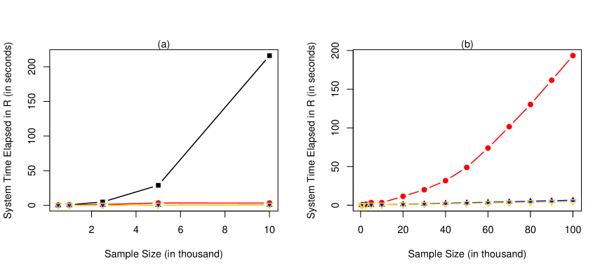
Figure 1: System time elapsed in seconds for fitting Case 3 with $\sigma=0.1$: (a) ALL (black filled square), RSR (red solid circle), EIGEN with $K=30$ (blue solid triangle), and Nyström with $K=30$ (gold triangle point down) with sample sizes $n=500,1000,2500,5000,10000$; (b) RSR (red solid circle), EIGEN with $K=30$ (blue solid triangle) and Nyström with $K=30$ (gold triangle point down) with sample sizes from 20000 to 100000 incremented by 10000.

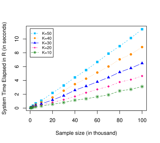
Figure 2: System time elapsed in seconds for fitting Case 3 with $\sigma=0.1$ by the EIGEN approach with $5$ different truncation parameters $K$.

Acknowledgements

This research was supported by a grant from the National Science Foundation (DMS-1507620). The authors acknowledge support from the Center for Scientific Computing from the CNSI, MRL: an NSF MRSEC (DMR1121053).

dcu

Appendix Appendix A Proof of Theorem 1

Lemma 1.

The approximation errors of $\tilde{\bm{c}}$ and $\tilde{\bm{d}}$ in terms of Euclidean norm are upper bounded as

$$\|\tilde{\bm{c}}-\bm{c}\|^{2} \leq\zeta_{1}B\tilde{B}\|\tilde{\Sigma}-\Sigma\|_{F}^{2},$$ (A.1)

$$\|\tilde{\bm{d}}-\bm{d}\|^{2} \leq\zeta_{2}\|\tilde{\Sigma}-\Sigma\|_{F}^{2}.$$ (A.2)

Proof.

The solutions to (4) are

$$\bm{c} =Q_{2}(Q_{2}^{\top}(\Sigma+n\lambda I)Q_{2})^{-1}Q_{2}^{\top}\bm{y},$$ (A.3)

$$\bm{d} =R^{-1}Q_{1}^{\top}(\bm{y}-(\Sigma+n\lambda I)\bm{c}).$$

The coefficients $\tilde{\bm{c}}$ and $\tilde{\bm{d}}$ have similar form as (A.3) with $\Sigma$ being replaced by $\tilde{\Sigma}$. Let $G=Q_{2}^{\top}(\Sigma+n\lambda I)Q_{2}$, $\tilde{G}=Q_{2}^{\top}(\tilde{\Sigma}+n\lambda I)Q_{2}$, and $FDF^{\top}$ and $\tilde{F}\tilde{D}\tilde{F}^{\top}$ be eigendecompositions of $Q_{2}^{\top}\Sigma Q_{2}$ and $Q_{2}^{\top}\tilde{\Sigma}Q_{2}$ respectively where $F$ and $\tilde{F}$ are $(n-p)\times(n-p)$ orthogonal matrices, and $D=\text{diag}(\lambda_{1,n},\ldots,\lambda_{n-p,n})$ and $\tilde{D}=\text{diag}(\tilde{\lambda}_{1,n},\ldots,\tilde{\lambda}_{n-p,n})$ are diagonal matrices with eigenvalues of $Q_{2}^{\top}\Sigma Q_{2}$ and $Q_{2}^{\top}\tilde{\Sigma}Q_{2}$. Then

$$\|\tilde{\bm{c}}-\bm{c}\|^{2} =\|Q_{2}[\tilde{G}^{-1}(\tilde{G}-G)G^{-1}]Q_{2}^{\top}\bm{y}\|^{2}$$

$$=\|Q_{2}\tilde{F}(\tilde{D}+n\lambda I)^{-1}(Q_{2}\tilde{F})^{\top}(\tilde{\Sigma}-\Sigma)Q_{2}F(D+n\lambda I)^{-1}(Q_{2}F)^{\top}\bm{y}\|^{2}$$

$$\leq\|Q_{2}\tilde{F}\|_{F}^{2}\|(\tilde{D}+n\lambda I)^{-1}\|_{F}^{2}\|(Q_{2}\tilde{F})^{\top}\|_{F}^{2}\|(\tilde{\Sigma}-\Sigma)\|_{F}^{2}\|Q_{2}F\|_{F}^{2}$$

$$\quad\cdot\|(D+n\lambda I)^{-1}\|_{F}^{2}\|F^{\top}Q_{2}^{\top}\bm{y}\|^{2}$$

$$=\|(\tilde{\Sigma}-\Sigma)\|_{F}^{2}\left(\sum_{k=1}^{n-p}(\tilde{\lambda}_{k,n}+n\lambda)^{-2}\right)\left(\sum_{k=1}^{n-p}(\lambda_{k,n}+n\lambda)^{-2}\right)\|Q_{2}\|_{F}^{6}\|Q_{2}^{\top}\bm{y}\|^{2}$$

$$\leq\|\tilde{\Sigma}-\Sigma\|_{F}^{2}B\tilde{B}\|Q_{2}\|_{F}^{6}\|Q_{2}^{\top}\bm{y}\|^{2}$$

$$=\zeta_{1}B\tilde{B}\|\tilde{\Sigma}-\Sigma\|_{F}^{2},$$ (A.4)

where we used the facts that the Frobenius norm of a vector equals its Euclidean norm, $\|Q_{2}F\|_{F}^{2}=\text{trace}(Q_{2}FF^{\top}Q_{2}^{\top})=\text{trace}(Q_{2}Q_{2}^{\top})=\|Q_{2}\|_{F}^{2}$, the first inequality holds because of submultiplicativity of the Frobenius norm, and the second inequality holds because of the triangle inequality and smoothing parameter $\lambda$ is non-negative.

Multiplying the first equation in (4) and the corresponding first equation for $\tilde{\bm{c}}$ and $\tilde{\bm{d}}$ by $T^{\top}$, and then taking the difference, we have $T^{\top}T(\tilde{\bm{d}}-\bm{d})+T^{\top}(\tilde{\Sigma}+n\lambda I)\tilde{\bm{c}}-T^{\top}(\Sigma+n\lambda I)\bm{c}=0$. Since $T^{\top}\bm{c}=\bm{0}$ and $T^{\top}\tilde{\bm{c}}=\bm{0}$ by the second equation in (4), we have $\tilde{\bm{d}}-\bm{d}=(T^{\top}T)^{-1}T^{\top}(\tilde{\Sigma}\tilde{\bm{c}}-\Sigma\bm{c})$ and

$$\|\tilde{\bm{d}}-\bm{d}\|^{2} =(\tilde{\Sigma}\tilde{\bm{c}}-\Sigma\bm{c})^{\top}A(\tilde{\Sigma}\tilde{\bm{c}}-\Sigma\bm{c})$$

$$\leq\lambda_{\text{max}}(A)\|\tilde{\Sigma}\bm{c}-\Sigma\bm{c}+\tilde{\Sigma}\tilde{\bm{c}}-\tilde{\Sigma}\bm{c}\|^{2}$$

$$\leq 2\lambda_{\text{max}}(A)\left[\|\bm{c}\|^{2}\|\tilde{\Sigma}-\Sigma\|_{F}^{2}+\|\tilde{\Sigma}\|_{F}^{2}\|\tilde{\bm{c}}-\bm{c}\|^{2}\right]$$

$$\leq 2\lambda_{\text{max}}(A)\left[\|\bm{c}\|^{2}\|\tilde{\Sigma}-\Sigma\|_{F}^{2}+\|\tilde{\Sigma}\|_{F}^{2}\zeta_{1}B\tilde{B}\|\tilde{\Sigma}-\Sigma\|_{F}^{2}\right]$$

$$=2\lambda_{\text{max}}(A)\left(\zeta_{1}B\tilde{B}\|\tilde{\Sigma}\|_{F}^{2}+\|\bm{c}\|^{2}\right)\|\tilde{\Sigma}-\Sigma\|_{F}^{2}$$

$$=\zeta_{2}\|\tilde{\Sigma}-\Sigma\|_{F}^{2},$$

where the second inequality holds by the Cauchy-Schwarz inequality, the third inequality holds because of submultiplicativity of the Frobenius norm, and the fourth inequality hold because of equation (A.4). ∎

Proof of Theorem 1.

Write the component $\hat{f}_{1}$ as

$$\hat{f}_{1}(x)=\sum_{i=1}^{n}c_{i}{\cal L}_{i(z)}R_{1}(x,z)=\sum_{k=1}^{\infty}\left[\delta_{k}\sum_{i=1}^{n}c_{i}{\cal L}_{i}\Phi_{k}\right]\Phi_{k}(x)\triangleq\sum_{k=1}^{\infty}a_{k}\Phi_{k}(x),$$

where $a_{k}=\delta_{k}\sum_{i=1}^{n}c_{i}{\cal L}_{i}\Phi_{k}$. Then the smoothing spline estimate has the form $\hat{f}(x)=\sum_{\nu=1}^{p}d_{\nu}\phi_{\nu}(x)+\sum_{k=1}^{\infty}a_{k}\Phi_{k}(x)$. Similarly, the low-rank approximation $\tilde{f}$ based on $\tilde{\Sigma}$ can be represented as $\tilde{f}(x)=\sum_{\nu=1}^{p}\tilde{d}_{\nu}\phi_{\nu}(x)+\sum_{k=1}^{K}\tilde{a}_{k}\Phi_{k}(x)$ where $\tilde{a}_{k}=\delta_{k}\sum_{i=1}^{n}\tilde{c}_{i}{\cal L}_{i}\Phi_{k}$. Since $\|\tilde{f}_{0}-\hat{f}_{0}\|^{2}_{2}=\int_{\mathcal{X}}(\sum_{\nu=1}^{p}\tilde{d}_{\nu}\phi_{\nu}(x)-\sum_{\nu=1}^{p}d_{\nu}\phi_{\nu}(x))^{2}dx=\|\tilde{\bm{d}}-\bm{d}\|^{2}$, then we have the upper bound for $\|\tilde{f}_{0}-\hat{f}_{0}\|^{2}_{2}$ by Lemma 1. For the approximation error $\left\|\tilde{f}_{1}-\hat{f}_{1}\right\|^{2}_{2}$, we have

$$\left\|\tilde{f}_{1}-\hat{f}_{1}\right\|^{2}_{2} =\int_{\mathcal{X}}\left[\sum_{k=1}^{K}\tilde{a}_{k}\Phi_{k}(x)-\sum_{k=1}^{\infty}a_{k}\Phi_{k}(x)\right]^{2}dx$$

$$=\sum_{k=1}^{K}\left(\tilde{a}_{k}-a_{k}\right)^{2}+\sum_{k=K+1}^{\infty}a_{k}^{2}$$

$$=\sum_{k=1}^{K}\delta_{k}^{2}\left(\sum_{i=1}^{n}(\tilde{c}_{i}-c_{i}){\cal L}_{i}\Phi_{k}\right)^{2}+\sum_{k=K+1}^{\infty}\delta_{k}^{2}\left(\sum_{i=1}^{n}c_{i}{\cal L}_{i}\Phi_{k}\right)^{2}$$

$$\leq\|\tilde{\bm{c}}-\bm{c}\|^{2}\left(\sum_{i=1}^{n}\sum_{k=1}^{K}\delta_{k}^{2}({\cal L}_{i}\Phi_{k})^{2}\right)+\|\bm{c}\|^{2}\left(\sum_{k=K+1}^{\infty}\sum_{i=1}^{n}\delta_{k}^{2}({\cal L}_{i}\Phi_{k})^{2}\right)$$

$$\leq n\kappa^{2}C_{K}\zeta_{1}B\tilde{B}\|\tilde{\Sigma}-\Sigma\|_{F}^{2}+n\kappa^{2}\|\bm{c}\|^{2}D_{K}$$

$$=\zeta_{3}\|\tilde{\Sigma}-\Sigma\|_{F}^{2}+n\kappa^{2}\|\bm{c}\|^{2}D_{K}.$$ (A.5)

Finally, using the fact that $\|\tilde{f}-\hat{f}\|_{2}^{2}\leq 2\|\tilde{f}_{0}-\hat{f}_{0}\|_{2}+2\|\tilde{f}_{1}-\hat{f}_{1}\|_{2}$, we have the upper bound for the overall function. ∎

Appendix Appendix B Proof of Theorem 2

Following similar arguments in the proof of Lemma 1, it can be shown that

$$\|\check{\bm{c}}-\tilde{\bm{c}}\|^{2} \leq\zeta_{1}\tilde{B}\check{B}\|\check{\Sigma}-\tilde{\Sigma}\|_{F}^{2},$$

$$\|\check{\bm{d}}-\tilde{\bm{d}}\|^{2} \leq\zeta_{2}^{\prime}\|\check{\Sigma}-\tilde{\Sigma}\|_{F}^{2}.$$

Furthermore, $\check{f}(x)=\check{f}_{0}(x)+\check{f}_{1}(x)=\sum_{\nu=1}^{p}\check{d}_{\nu}\phi_{\nu}(x)+\sum_{k=1}^{K}\check{a}_{k}\check{\Phi}_{k}(x)$ where $\check{a}_{k}=\check{\delta}_{k}\sum_{i=1}^{n}\check{c}_{i}{\cal L}_{i}\check{\Phi}_{k}$. The upper bound for $\|\check{f}_{0}-\tilde{f}_{0}\|_{2}^{2}$ can be derived similarly as in the proof of Theorem 1. We now derive the upper bound for $\|\check{f}_{1}-\tilde{f}_{1}\|_{2}^{2}$.

$$\|\check{f}_{1}-\tilde{f}_{1}\|_{2}^{2} =\left\|\sum_{k=1}^{K}\check{a}_{k}\check{\Phi}_{k}(x)-\sum_{k=1}^{K}\tilde{a}_{k}\Phi_{k}(x)\right\|_{2}^{2}$$

$$\leq 2\left\|\sum_{k=1}^{K}\check{a}_{k}\check{\Phi}_{k}(x)-\sum_{k=1}^{K}\check{a}_{k}\Phi_{k}(x)\right\|_{2}^{2}+2\left\|\sum_{k=1}^{K}\check{a}_{k}\Phi_{k}(x)-\sum_{k=1}^{K}\tilde{a}_{k}\Phi_{k}(x)\right\|_{2}^{2}$$

$$=2\left\|\sum_{k=1}^{K}\check{a}_{k}\left(\check{\Phi}_{k}(x)-\Phi_{k}(x)\right)\right\|_{2}^{2}+2\sum_{k=1}^{K}(\check{a}_{k}-\tilde{a}_{k})^{2}$$

$$=2(I+II).$$

Moreover,

$$I =\int_{\mathcal{X}}\left(\sum_{k=1}^{K}\check{a}_{k}\left(\check{\Phi}_{k}(x)-\Phi_{k}(x)\right)\right)^{2}dx$$

$$\leq\left(\sum_{k=1}^{K}\check{a}_{k}^{2}\right)\left(\sum_{k=1}^{K}\left\|\check{\Phi}_{k}(x)-\Phi_{k}(x)\right\|_{2}^{2}\right)$$

$$=\sum_{k=1}^{K}\check{\delta}_{k}^{2}\left(\sum_{i=1}^{n}\check{c}_{i}{\cal L}_{i}\check{\Phi}_{k}\right)^{2}\left(\sum_{k=1}^{K}\left\|\check{\Phi}_{k}(x)-\Phi_{k}(x)\right\|_{2}^{2}\right)$$

$$\leq\sum_{k=1}^{K}\check{\delta}_{k}^{2}\left(\sum_{i=1}^{n}\check{c}_{i}^{2}\right)\left(\sum_{i=1}^{n}{\cal L}_{i}\check{\Phi}_{k}^{2}\right)\left(\sum_{k=1}^{K}\left\|\check{\Phi}_{k}(x)-\Phi_{k}(x)\right\|_{2}^{2}\right)$$

$$\leq\|\check{\bm{c}}\|^{2}n\kappa^{\prime 2}\left(\sum_{k=1}^{K}\check{\delta}_{k}^{2}\right)\left(\sum_{k=1}^{K}\left\|\check{\Phi}_{k}(x)-\Phi_{k}(x)\right\|_{2}^{2}\right)$$

$$=\zeta_{4}\sum_{k=1}^{K}\left\|\check{\Phi}_{k}(x)-\Phi_{k}(x)\right\|_{2}^{2}.$$ (A.6)

The first and second inequalities hold by the Cauchy-Schwarz inequality, and the third equality holds because of the boundness assumption of ${\cal L}_{i}\check{\Phi}_{k}$.

$$II =\sum_{k=1}^{K}\left(\check{\delta}_{k}\sum_{i=1}^{n}\check{c}_{i}{\cal L}_{i}\check{\Phi}_{k}-\delta_{k}\sum_{i=1}^{n}\tilde{c}_{i}{\cal L}_{i}\Phi_{k}\right)^{2}$$

$$\leq 3\sum_{k=1}^{K}\left(\check{\delta}_{k}\sum_{i=1}^{n}\check{c}_{i}{\cal L}_{i}\check{\Phi}_{k}-\check{\delta}_{k}\sum_{i=1}^{n}\check{c}_{i}{\cal L}_{i}\Phi_{k}\right)^{2}+3\sum_{k=1}^{K}\left(\check{\delta}_{k}\sum_{i=1}^{n}\check{c}_{i}{\cal L}_{i}\Phi_{k}-\delta_{k}\sum_{i=1}^{n}\check{c}_{i}{\cal L}_{i}\Phi_{k}\right)^{2}$$

$$\qquad+3\sum_{k=1}^{K}\left(\delta_{k}\sum_{i=1}^{n}\check{c}_{i}{\cal L}_{i}\Phi_{k}-\delta_{k}\sum_{i=1}^{n}\tilde{c}_{i}{\cal L}_{i}\Phi_{k}\right)^{2}$$

$$\leq 3\|\check{\bm{c}}\|^{2}\sum_{k=1}^{K}\left[\check{\delta}_{k}^{2}\sum_{i=1}^{n}({\cal L}_{i}\check{\Phi}_{k}-{\cal L}_{i}\Phi_{k})^{2}\right]+3n\kappa^{2}\|\check{\bm{c}}\|^{2}\sum_{k=1}^{K}(\check{\delta}_{k}-\delta_{k})^{2}+3n\kappa^{2}C_{K}\|\check{\bm{c}}-\tilde{\bm{c}}\|^{2},$$

where the first inequality holds by the Cauchy-Schwartz inequality. Combining $I$, $II$ and upper bound for $\|\check{\bm{c}}-\tilde{\bm{c}}\|^{2}$ we have the upper bound for $\|\check{f}_{1}-\tilde{f}_{1}\|_{2}^{2}$.

Finally, using the fact that $\|\check{f}-\tilde{f}\|_{2}^{2}\leq 2\|\check{f}_{0}-\tilde{f}_{0}\|_{2}+2\|\check{f}_{1}-\tilde{f}_{1}\|_{2}$, we have the upper bound for the overall function.

References

• [1] \harvarditem[Alaoui and Mahoney]Alaoui and Mahoney2015alaoui2015fast Alaoui, A. and Mahoney, M. W. (2015). Fast randomized kernel ridge regression with statistical guarantees, Advances in Neural Information Processing Systems, pp. 775–783.
• [2] \harvarditem[Amini and Wainwright]Amini and Wainwright2012amini2012 Amini, A. A. and Wainwright, M. J. (2012). Sampled forms of functional PCA in reproducing kernel Hilbert spaces, Ann. Statist. 40(5): 2483–2510.
• [3] \harvarditem[Bach]Bach2013Bach13 Bach, F. (2013). Sharp analysis of low-rank kernel matrix approximations, in S. Shalev-Shwartz and I. Steinwart (eds), Proceedings of the 26th Annual Conference on Learning Theory, Vol. 30 of Proceedings of Machine Learning Research, PMLR, Princeton, NJ, USA, pp. 185–209.
• [4] \harvarditem[Baker]Baker1977baker1977numerical Baker, C. (1977). The Numerical Treatment of Integral Equations, Monographs on Numerical Analysis Series, Oxford : Clarendon Press.
• [5] \harvarditem[Cortes et al.]Cortes, Mohri and Talwalkar2010cortes2010impact Cortes, C., Mohri, M. and Talwalkar, A. (2010). On the impact of kernel approximation on learning accuracy, in Y. W. Teh and M. Titterington (eds), Proceedings of the Thirteenth International Conference on Artificial Intelligence and Statistics, Vol. 9 of Proceedings of Machine Learning Research, JMLR Workshop and Conference Proceedings, Chia Laguna Resort, Sardinia, Italy, pp. 113–120.
• [6] \harvarditem[Delves and Mohamed]Delves and Mohamed1988delves1988computational Delves, L. and Mohamed, J. (1988). Computational Methods for Integral Equations, Cambridge University Press.
• [7] \harvarditem[Fine and Scheinberg]Fine and Scheinberg2002fine2002efficient Fine, S. and Scheinberg, K. (2002). Efficient SVM training using low-rank Kernel representations, Journal of machine learning research 2(2): 243–264.
• [8] \harvarditem[Girolami]Girolami2002Girolami:2002:OSD:638929.638938 Girolami, M. (2002). Orthogonal Series Density Estimation and the Kernel Eigenvalue Problem, Neural Comput. 14(3): 669–688.
• [9] \harvarditem[Gu]Gu2009gss Gu, C. (2009). General Smoothing Splines, Available at http://cran.r-project.org.
• [10] \harvarditem[Gu]Gu2013gu2013smoothing Gu, C. (2013). Smoothing spline ANOVA models, Vol. 297, Springer Science & Business Media.
• [11] \harvarditem[Hastie]Hastie1996pseudospline Hastie, T. (1996). Pseudosplines, Journal of the Royal Statistical Society: Series B 58: 379–396.
• [12] \harvarditem[Kim and Gu]Kim and Gu2004kim2004smoothing Kim, Y.-J. and Gu, C. (2004). Smoothing spline gaussian regression: More scalable computation via efficient approximation, Journal of the Royal Statistical Society. Series B (Statistical Methodology) 66(2): 337–356.
• [13] \harvarditem[Lanczos]Lanczos1950Lanczos:1950zz Lanczos, C. (1950). An iteration method for the solution of the eigenvalue problem of linear differential and integral operators, J. Res. Natl. Bur. Stand. B 45: 255–282.
• [14] \harvarditem[Lindstrom and Bates]Lindstrom and Bates1988lindstrom1988 Lindstrom, M. J. and Bates, D. M. (1988). Newton-Raphson and EM Algorithms for Linear Mixed-Effects Models for Repeated-Measures Data, Journal of the American Statistical Association 83(404): 1014–1022.
• [15] \harvarditem[Ma et al.]Ma, Huang and Zhang2015ma2015efficient Ma, P., Huang, J. Z. and Zhang, N. (2015). Efficient computation of smoothing splines via adaptive basis sampling, Biometrika 102(3): 631–645.
• [16] \harvarditem[Melkman and Micchelli]Melkman and Micchelli1978melkman1978 Melkman, A. A. and Micchelli, C. A. (1978). Spline spaces are optimal for $L^{2}\,\,n$-width, Illinois J. Math. 22(4): 541–564.
• [17] \harvarditem[Micchelli and Wahba]Micchelli and Wahba1979micchelli1979design Micchelli, C. A. and Wahba, G. (1979). Design Problems for Optimal Surface Interpolation, Technical report, Department of Statistics, University of Wisconsin, Madison.
• [18] \harvarditem[Pinheiro et al.]Pinheiro, Bates, DebRoy, Sarkar and R Core Team2017nlme Pinheiro, J., Bates, D., DebRoy, S., Sarkar, D. and R Core Team (2017). nlme: Linear and Nonlinear Mixed Effects Models. R package version 3.1-131.
• [19] \harvarditem[Santin and Schaback]Santin and Schaback2016Santin2016 Santin, G. and Schaback, R. (2016). Approximation of eigenfunctions in kernel-based spaces, Advances in Computational Mathematics 42(4): 973–993.
• [20] \harvarditem[Wahba]Wahba1990wahba1990spline Wahba, G. (1990). Spline models for observational data, Vol. 59, Siam.
• [21] \harvarditem[Wang]Wang1998Wang98 Wang, Y. (1998). Mixed-effects smoothing spline ANOVA, Journal of the Royal Statistical Society: Series B 60: 159–174.
• [22] \harvarditem[Wang]Wang2011wang2011smoothing Wang, Y. (2011). Smoothing splines: methods and applications, CRC Press.
• [23] \harvarditem[Wang and Ke]Wang and Ke2002assist Wang, Y. and Ke, C. (2002). ASSIST: A Suite of S-plus functions Implementing Spline smoothing Techniques, Available at http://cran.r-project.org.
• [24] \harvarditem[Williams and Seeger]Williams and Seeger2001williams2001 Williams, C. K. I. and Seeger, M. (2001). Using the Nyström Method to Speed Up Kernel Machines, in T. K. Leen, T. G. Dietterich and V. Tresp (eds), Advances in Neural Information Processing Systems 13, MIT Press, pp. 682–688.
• [25] \harvarditem[Wood]Wood2003wood2003thinplate Wood, S. N. (2003). Thin Plate Regression Splines, Journal of the Royal Statistical Society. Series B (Statistical Methodology) 65(1): 95–114.
• [26] \harvarditem[Xu and Wang]Xu and Wang2018xu2018 Xu, D. and Wang, Y. (2018). Divide and Recombine Approaches for Fitting Smoothing Spline Models with Large Datasets, Journal of Computational and Graphical Statistics 27(3): 677–683.
• [27] \harvarditem[Yang et al.]Yang, Pilanci and Wainwright2017Yang17 Yang, Y., Pilanci, M. and Wainwright, M. (2017). Randomized sketches for kernels: Fast and optimal nonparametric regression, Annals of Statistics 45: 991–1023.
• [28] \harvarditem[Zwald and Blanchard]Zwald and Blanchard2006zwald2006convergence Zwald, L. and Blanchard, G. (2006). On the convergence of eigenspaces in kernel principal component analysis, Advances in neural information processing systems, pp. 1649–1656.
• [29]