Robust cooperative synchronization of homogeneous agents with delays on directed communication graphs

Abstract

This study deals with analysis and control of cooperative synchronization for identical agents interacting on a directed graph topology. The agents are considered to have general continuous linear time-invariant dynamics with homogeneous communication and/or control delays. An LMI approach based on a Lyapunov-Krasovskii functional is proposed, together with the synchronizing region concept, which decouples the single-agent dynamics from the detailed graph topology. Moreover, the conventional notion of synchronizing region is here extended by an LMI relaxation utilizing quasi-convex characteristic of the problem. This leads to less conservative results for the region of graph matrix eigenvalues in the complex domain, where the synchronization is guaranteed. The proposed method to calculate the allowable delay bound for synchronization is also less conservative as compared to the results from the literature. Furthermore, two designs for distributed state-feedback control are suggested. The precise delay value and the detailed graph topology need not be known for their application; it suffices only to know the upper bound on the delay and the approximate region where the Laplacian eigenvalues lie. Specific improvements over the results existing in the literature are demonstrated by a numerical example, which validates the proposed approaches.

1 Introduction

The consensus/synchronization problem for multi-agent systems (MASs) has recently been a very attractive research field (Cao et al. 2013; Qin et al. 2017). One of the main reasons for this is the broad area of its application to complex engineering tasks such as flocking/formation control of mobile robots and vehicles, see Oh, Park, and Ahn (2015). Early works such as presented in Olfati-Saber and Murray (2004); Olfati-Saber, Fax, and Murray (2007) focused on consensus problem for one-dimensional agents without a leader, where all agents converge to a final consensus value determined by their precise initial conditions. On the other hand, pinning a group of agents with general higher-order dynamics to a leader is considered in Wang and ChenGuanrong (2002) to synchronize all nodes to the leader node’s trajectory for all initial conditions. Such synchronization problem, also called as cooperative tracking, was studied for general linear time-invariant (LTI) agents in Fax and Murray (2004); Li, Duan, and Chen (2011); Li et al. (2010) without pinning and in Zhang, Lewis, and Das (2011) for pinning control, utilizing Lyapunov stability theory. References Li, Duan, and Chen (2011); Li et al. (2010); Zhang, Lewis, and Das (2011) have considered decoupling the single-agent dynamics from the detailed network topology, through the concept of synchronizing region, which greatly simplifies the design. The synchronizing region refers to the region in the complex plane for the graph matrix eigenvalues such that synchronization of a MAS is guaranteed. The idea of synchronizing region approach was first presented in Pecora and Carrol (1998) for synchronization of identical coupled oscillators, where a master stability function is introduced to reduce effects of graph topology to robust stability of single-agent closed-loop dynamics. Due to this simplifying characteristic, the synchronizing region approach has been adapted for the solution of several MAS problems, e.g. optimal control in Hengster-Movric and Lewis (2014) and $H_{\infty}$ synchronization in Hengster-Movric, Lewis, and Šebek (2015).

Among the studies on synchronization of MASs, time-delay phenomena have been widely investigated since delays are unavoidable in communication links and quite common in control action. Thus, delays must be taken into account in analysis, and robustness to delays must be guaranteed for any realistic cooperative distributed control protocol. There are two main general approaches for analysis of time-delay systems (TDSs) (Gu, Kharitonov, and Chen 2003): frequency domain techniques and time-domain approach based on Lyapunov-Razumikhin functions (LRFs) or Lyapunov-Krasovskii functionals (LKFs). The first results based on Nyquist plots were given in Olfati-Saber and Murray (2004) for consensus of single-integrator agents on a fixed undirected graph topology, with a uniform delay. For the same problem on a digraph topology, a systematic approach in frequency domain for the analysis of delay margin guaranteeing consensus was proposed in Sipahi and Qiao (2011), and a distributed robust consensus control was proposed in Lin, Jia, and Li (2008) to achieve the desired $H_{\infty}$ performance. There are also more recent papers utilizing different frequency domain techniques for consensus of MASs with second-order agents on digraphs, e.g. for double-integrator dynamics in Cepeda-Gomez and Olgac (2013), and for general second-order agents in Hou et al. (2017). Both Cepeda-Gomez and Olgac (2013) and Hou et al. (2017) consider decoupling/decomposition of the dynamics depending on eigenvalues of matrices describing the communication topology, e.g. Laplacian eigenvalues in Hou et al. (2017), so that the analysis can be performed with a set of low-order subsystems. Another remarkable work based on an inequality technique for second-order MASs with multiple time-varying delays is Zhu and Cheng (2010) where the decomposition of the global networked dynamics is considered. Beside the MAS with low-order single-agents mentioned briefly above, several papers were published on consensus/synchronization problem of high-order linear agents with delays. In Münz, Papachristodoulou, and Allgöwer (2010, 2012), robustness of consensus protocols to non-uniform constant feedback delays are investigated for identical and non-identical single-input single-output (SISO) agents with eigenvalues in the open left-half plane, networked on undirected topology. Consensus among multi-input multi-output (MIMO) identical agents on directed graphs with uniform constant communication delays has been studied in Wang et al. (2013), where the proposed approach is valid only for agents with eigenvalues in the closed left-half plane. Frequency domain techniques utilized in Münz, Papachristodoulou, and Allgöwer (2010, 2012); Wang et al. (2013) impose restrictions on single-agent dynamics such as requiring only SISO or only (marginally) stable agents. Predictor-based feedback protocols for consensus of MAS on directed graphs in the presence of communication and input delays have been proposed in Zhou and Lin (2014). Since predictor-based feedback suffers from implementation problems (Zhou, Lin, and Duan 2012), a truncated predictor approach has also been proposed in Zhou and Lin (2014), however it remains valid only for agents which are at most critically unstable just as in Wang et al. (2013). As for the time-domain methods, allowable uniform communication delay bound for consensus of general linear MASs on undirected networks, has been studied via an LKF approach in Zhang and Tian (2014). Based on LKFs, several papers such as (Karimi 2011; Karimi, Zapateiro, and Luo 2012; Yi-Ping and Bi-Feng 2015) worked on general synchronization under delays, however in a centralized manner treating the entire MAS system as a whole. For identical agents on directed graphs with general LTI dynamics and uniform input delays, an algebraic Riccati equation (ARE) solution based on LRF has been proposed for cooperative synchronization in Hengster-Movric et al. (2015), with pinning control and synchronizing region approach. Very recently, allowable delay bound for the same problem without pinning on arbitrary network topology has been studied in Sheng et al. (2018), however assuming the network has closed strong components. Another recent paper Zhang, Saberi, and Stoorvogel (2018) proposes a parametric ARE-based solution for consensus of MAS with non-uniform constant communication delays on connected undirected graphs, where the tolerable delay bound is known, however the agents are assumed to be at most critically unstable. With the exception of Hengster-Movric et al. (2015), the proposed distributed methods in the mentioned papers impose restrictions on single-agent dynamics or on graph topology, even if the delays are uniform and constant.

In this paper, we consider synchronization of homogeneous general LTI agents with uniform constant communication (and/or control) delays. Agents are assumed interacting on a directed graph topology, thus general networks are considered in contrast to Münz, Papachristodoulou, and Allgöwer (2010); Zhang and Tian (2014); Zhang, Saberi, and Stoorvogel (2018) dealing only with undirected graphs. The underlying graph is assumed to have a directed spanning tree, which is a common and a mild assumption in the MAS literature. This is also a more general condition, compared to requiring the existence of closed strong components in Sheng et al. (2018), where only the allowable delay bound is analyzed. There are no restrictions on agent dynamics as in Münz, Papachristodoulou, and Allgöwer (2010); Wang et al. (2013); Zhou and Lin (2014), except for requiring single-agent stabilizability, which is inherently necessary for synchronization. Here we bring together, for the first time, the synchronizing region concepts of cooperative control, Lyapunov-Krasovskii delay-dependent stability analysis, and methods familiar from robust control to present a less conservative robust distributed control design. An LKF based LMI approach is thus proposed for both the analysis of cooperative synchronization in delayed MAS and the synchronization control design. Utilizing the well-known results of synchronizing region concept, we deal with robust stability of the single-agent closed-loop dynamics, where the uncertain parameters stand for the graph matrix eigenvalues and the delay, instead of dealing with the entire global networked dynamics, as e.g. in Karimi (2011); Karimi, Zapateiro, and Luo (2012); Yi-Ping and Bi-Feng (2015). The proposed method relies on a newly revealed quasi-convexity property with respect to graph matrix eigenvalues, which is found to be crucial for our main development. Namely, based on quasi-convexity, a novel approach is presented for analyzing and treating the graph matrix eigenvalues. The proposed approach relaxes the conventional synchronizing region methodology in Hengster-Movric et al. (2015), which is found to be quite conservative both for delay bound and network topology requirements. This relaxation relies on using multiple LKFs and taking advantage of the quasi-convexity. In particular, we propose a unified approach for determining the allowable delay bound and the synchronizing region for any given state-feedback controller, and designing distributed cooperative state-feedback controls. Only the delay upper bound and the approximate region in the complex plane where the Laplacian eigenvalues should reside need to be known.

The main contributions of this paper are summarized as follows:

1. A new approach to reveal the effects of network topology under communication/control delays is proposed in the spirit of synchronizing region. The synchronization criterion for delay bound and graph matrix eigenvalues is relaxed compared to the classical synchronizing region approach in Hengster-Movric et al. (2015), leading to considerably reduced conservatism.

2. An efficient algorithm to estimate the delay-dependent synchronizing region is given based on feasibility of LMIs.

3. A direct robust cooperative synchronization control design is provided without tuning a coupling gain, as opposed to most conventional synchronizing region designs, e.g. in Li et al. (2010); Zhang, Lewis, and Das (2011); Hengster-Movric et al. (2015).

The paper is organized as follows. Section 2 provides notation, graph properties, and quasi-convexity preliminaries. Section 3 presents the MAS dynamics and the problem statements. The proposed LKF based LMI approach to find the allowable delay bound is given in Section 4. Based on the main results in Section 4, an efficient algorithm to obtain an estimate of the delay-dependent synchronizing region and two approaches for distributed state-feedback control design are given in Sections 5 and 6, respectively. The results and improvements are verified via numerical simulations in Section 7, and Section 8 concludes the paper.

2 Preliminaries

Throughout the paper, $\mathbb{R}^{n}$ denotes the n-dimensional real Euclidean space, and $\mathbb{R}^{n\times m}$ is the set of all $n\times m$ matrices. $\mathbb{C}$ stands for the complex numbers. For any complex number $z$, we denote its conjugate by $z^{*}$. The notation $P\succ 0$, for $P\in\mathbb{R}^{n\times n}$ means that $P$ is symmetric and positive definite. The symmetric elements of symmetric (or hermitian) matrices are denoted by $\star$. The notation $P^{H}$ stands for the hermitian (or conjugate) transpose of the matrix $P$. The space of functions $\phi:[-h,0]\rightarrow\mathbb{R}^{n}$, which are absolutely continuous on $[-h,0]$, and have square integrable first order derivatives, i.e. $\dot{\phi}\in L_{2}(-h,0)$, is denoted by $W[-h,0]$ with the norm $\|\phi\|_{W}={\text{max}}_{\theta\in[-h,0]}|\phi(\theta)|+[\textstyle\int_{-h}^{0}|\dot{\phi}(\theta)|^{2}ds]^{1/2}$. For $x:\mathbb{R}\rightarrow\mathbb{R}^{n}$, we denote $x_{t}(\theta)\triangleq x(t+\theta),\;\theta\in[-h,0]$.

2.1 Graph Theory & Properties

$\mathcal{G}=(\mathcal{V},\mathcal{E})$ represents a graph with $N$ nodes $\mathcal{V}=\{v_{1},\ldots,v_{N}\}$ and a set of edges $\mathcal{E}\subseteq\mathcal{V}\times\mathcal{V}$. An edge rooted at $v_{j}$ and ended at $v_{i}$ is denoted by ($v_{j},v_{i}$). We consider only simple graphs, i.e. there are no repeated edges or self-loops. A sequence of successive edges from $v_{i}$ to $v_{j}$ in the form $\{(v_{i},v_{k}),(v_{k},v_{l}),\ldots,(v_{m},v_{j})\}$ is called as directed path. A graph is strongly connected if every two nodes can be joined by a directed path. The graph is said to contain a directed spanning tree if there exists a node $v_{0}$ such that every other node in $\mathcal{V}$ can be connected to $v_{0}$ by a directed path starting from $v_{0}$. Such a special node is then called a root node denoted by $v_{i_{r}}$.

Adjacency (connectivity) matrix is denoted as $E=\{\alpha_{ij}\}$, with $\alpha_{ij}>0$ if $(v_{j},v_{i})\in\mathcal{E}$ and $\alpha_{ij}=0$ otherwise. The set of neighbors of node $v_{i}$ is denoted as $\mathcal{N}_{i}=\{v_{j}:(v_{j},v_{i})\in\mathcal{E}\}$, i.e. the set of nodes with edges coming into $v_{i}$. $D=\text{diag}(d_{1},\ldots,d_{N})$ with $d_{i}=\textstyle{\sum}\alpha_{ij}$ the weighted degree of node $i$ denotes the in-degree matrix for $\mathcal{G}$. Then the (graph) Laplacian matrix is defined as $L=D-E$. The Laplacian matrix $L$ has a simple zero eigenvalue if and only if the digraph contains a spanning tree.

2.2 Convex Polytopes and Quasi-convexity

A compact and convex polytope, denoted by $\Delta_{M}$, is characterized also by the set of its vertices, $V:=\{\nu_{1},\ldots,\nu_{M}\}$. We denote the operation of taking the convex hull by ${\mathbf{co}}\{\cdot\}$, and the operation of taking the set of vertices by ${\mathbf{vert}}\{\cdot\}$. So, by definition $\Delta_{M}={\mathbf{co}}\{V\}$ and $V={\mathbf{vert}}\{\Delta_{M}\}$. Then we have the following.

Definition 1 (Quasi-convexity, Apkarian and Tuan (2000)).

Let $S$ be a convex subset of $\mathbb{R}^{n}$. A function $f:S\rightarrow\mathbb{R}$ is quasi-convex if for all $u,v$ in $S$ and $\alpha\in[0,1]$, $f(\alpha u+(1-\alpha)v)\leq{\rm{max}}\{f(u),f(v)\}$.

Theorem 1 (Multi-quasi-convexity, Apkarian and Tuan (2000)).

Consider a compact convex polytope $\Delta_{M}$ in $\mathbb{R}^{n}$ and the directions $b_{1},\ldots,b_{q}$ determined by the edges of $\Delta_{M}$. Assume that for any $x$ in $\Delta_{M}$, the function $f$ is quasi-convex on the line segments

$$L_{b_{i}}(x):=\{z\in\Delta_{M}:z=x+\xi b_{i},\xi\in\mathbb{R}\},i=1,\ldots,q.$$

Then, $f$ has a maximum over $\Delta_{M}$ at a vertex of $\Delta_{M}$.

3 Multi-agent System and Problem Statement

We consider a set of $N$ homogenous agents having general LTI dynamics with control input delay, $\tau_{\rm{in}}\geq 0$

$$\dot{x}_{i}(t)=Ax_{i}(t)+Bu_{i}(t-\tau_{\rm{in}}),\quad i=1,\ldots,N,$$ (1)

and a leader system with autonomous dynamics

$$\dot{x}_{0}(t)=Ax_{0}(t)$$ (2)

where $x_{0},x_{i}\in\mathbb{R}^{n}$, $u_{i}\in\mathbb{R}^{m}$ are states and inputs, respectively, and $A\in\mathbb{R}^{n\times n}$ and $B\in\mathbb{R}^{n\times m}$. One can consider the leader system (2) as an exosystem serving as a command generator (Zhang, Lewis, and Das 2011), which is to be tracked by all the agents. For that purpose, the leader pins to a subset of agents.

The distributed cooperative tracking (or synchronization) control goal is to find $u_{i}$ depending on $x_{i},\;x_{j\in\mathcal{N}_{i}}$ such that all agents’ states asymptotically synchronize to the trajectory of the leader node (2), i.e. $\parallel x_{i}(t)-x_{0}(t)\parallel\rightarrow 0$ as $t\rightarrow\infty$. We consider the distributed state-feedback control of the form

$$u_{i}(t)=Ke_{i}(t),$$ (3)

applied to each agent, $\forall i$, with the delayed local neighborhood error

$$e_{i}(t)=\sum_{j}{\alpha_{ij}\left[x_{j}(t-\tau_{\rm{c}})-x_{i}(t-\tau_{\rm{c}})\right]+g_{i}\left[x_{0}(t-\tau_{\rm{c}})-x_{i}(t-\tau_{\rm{c}})\right]}$$ (4)

where $\alpha_{ij}$ are the elements of adjacency matrix $E$ of the directed graph topology of the MAS, $g_{i}\geq 0$ are the pinning gains that are nonzero only for a few agents directly connected to the leader, and $\tau_{\rm{c}}\geq 0$ represents the communication delay. Then, the closed-loop dynamics of each agent with the control (3) becomes

$$\dot{x}_{i}(t)=Ax_{i}(t)+BKe_{i}(t-\tau_{\rm{in}}).$$ (5)

For future LKF analysis, we assume that the initial conditions of the MAS (1) are $x_{it}(\theta)\in\phi$ and $u_{it}(\theta)\in\phi$, $\theta\in[-\tau,0]$, where $\tau=\tau_{\rm{in}}+\tau_{\rm{c}}$ is the total delay. Defining the synchronization error of an agent as $\delta_{i}=x_{i}-x_{0}$ and considering the total delay $\tau$, the global synchronization error dynamics of the networked system can be written straightforwardly as

$$\dot{\delta}(t)=\left(I_{N}\otimes A\right)\delta(t)-(L+G)\otimes BK\delta(t-\tau),$$ (6)

where $\delta(t)=\left[\delta_{1}^{T}(t)\ldots\delta_{N}^{T}(t)\right]^{T}\in\mathbb{R}^{N\cdot n}$, and $G={\rm{diag}}(g_{1},\ldots,g_{N})$ is the pinning gain matrix. Notice that the pinned (graph) Laplacian matrix ($L+G$) appears in synchronization dynamics (6), instead of the Laplacian matrix ($L$) itself. Let us here present the assumption on the graph topology that holds throughout the paper, and a relevant lemma on the pinned Laplacian matrix which is important and well-known.

Assumption 1.

The digraph $\mathcal{G}$ contains a directed spanning tree with at least one nonzero pinning gain into a root node.

Lemma 1.

(Wang and ChenGuanrong 2002; Zhang, Lewis, and Das 2011) Under Assumption 1, $L+G$ is non-singular with all the eigenvalues ($\lambda_{j}$) in the open right-half complex plane, i.e. $\lambda_{j}\in\mathbb{C}_{+}$, $j=1,\ldots$,N.

For the synchronization of the MAS (1–4), the global synchronization error dynamics (6) is required to be asymptotically stable, i.e. $\lim_{t\to\infty}\delta(t)\rightarrow 0$. Thus, we state the considered problems as follows:

Problem 1.

Find the allowable delay bound ($\tau\leq h$) in (6) such that the synchronization of the MAS (1–4) is guaranteed for all $\tau\in[0,h]$, for a given specific $K$.

Problem 2.

Find the region for the eigenvalues of $L+G$ in the complex plane where the MAS synchronization with (1–4) is guaranteed for all $\tau\in[0,h]$ and for a given specific $K$.

Problem 3.

Provide a design method, namely find a distributed cooperative state-feedback control law (3) with (4) $\forall\tau\in[0,h]$ such that the states of the agents (1) synchronize to the states of the leader (2), for a given delay bound $(h)$ and for a given region of the eigenvalues of $L+G$.

Remark 1.

We assume that the total delay $\tau$ is constant and uniform for each communication link. Even though this assumption usually does not fit the most realistic cases, nevertheless it is a general assumption in the literature, see e.g. Olfati-Saber and Murray (2004); Zhou and Lin (2014); Yi-Ping and Bi-Feng (2015); Hengster-Movric et al. (2015); Sheng et al. (2018); Wang and Ding (2016), allowing concise theoretical developments, in particular focusing on single-agent dynamics instead of the entire MAS. Moreover, from the practical side, even if the delays are originally found to be unequal, they can be made uniform through specific implementation by using time-stamps and inserting artificial delays on the signals received from neighboring agents, to guarantee the results presented in this work remain valid.

Note that (6) is a retarded functional differential equation (RFDE), which has infinitely many characteristic roots. The stability and stabilization problem of TDSs is known to be NP-hard (Gu, Kharitonov, and Chen 2003). As the number of agents $N$ increases, i.e. the dimension of RFDE (6) gets higher, the computational load for the analysis/synthesis problem of the TDS becomes cumbersome. This is so on large scale networks even for the delay-free case. To avoid such difficulties and to reveal the effects of graph topology on the global dynamics, we resort to synchronizing region approach (Li, Duan, and Chen 2011; Li et al. 2010; Zhang, Lewis, and Das 2011).

The key idea in the synchronizing region approach introduced below is to reduce the global synchronization error dynamics of dimension $Nn$ to $N$ $n$-dimensional systems that depend on the eigenvalues of the graph matrix. With a coordinate transformation matrix, which leads to the transformed graph matrix in the upper triangular form, the global dynamics can be decomposed with respect to the graph topology, i.e. the eigenvalues of $L$ (or $L+G$), see Fax and Murray (2004); Zhang, Lewis, and Das (2011). This decomposition was extended to the leader follower MAS synchronization problem with uniform constant delay in Hengster-Movric et al. (2015) as in the following lemma, under Assumption 1.

Lemma 2.

(Hengster-Movric et al. 2015) The trivial solution of the system (6) is asymptotically stable if and only if the trivial solutions of the systems

$$\dot{x}(t)=Ax(t)-\lambda_{j}BKx(t-\tau),\;j=1,\ldots,N$$ (7)

each having the order of a single-agent, where $\lambda_{j}$ are the eigenvalues of L+G, are asymptotically stable $\forall j$.

As a result of Lemma 2 for the synchronization problem, instead of analyzing (6) with higher dimension ($Nn$), one can investigate the robust stability of a lower dimension ($n$) system (7). This also provides an insight into graph topology both for analysis and design.

Note that (7) is a complex RFDE in $\mathbb{C}^{n}$ depending on $\lambda_{j}$. Thus, to provide a convenient representation from the perspective of robustness, let us rewrite (7) in the form,

$$\dot{x}(t)=Ax(t)+\sigma A_{d}x(t-\tau),$$ (8)

where $A_{d}:=-BK$, and $\sigma\in\mathbb{C}$. Then, the following definition is given to investigate the robust stability of (8) with respect to $\sigma$ and $\tau$.

Definition 2.

Given a complex RFDE as in (8), the delay-dependent synchronizing region (DSR) is a subset of the complex plane $\mathbb{C}$ depending on the delay bound

$$S_{c}(h)=\left\{\sigma\in\mathbb{C}:Ax(t)+\sigma A_{d}x(t-\tau){\rm{\;is\;asymptotically\;stable\;}}\forall\tau\in[0,h]\right\}.$$ (9)

Note that Definition 2 slightly differs from the one in Hengster-Movric et al. (2015), since we consider the synchronizing region where the robust stability for any $\tau\in[0,h]$ is guaranteed. Definitely, the DSR depends also on the system dynamics ($A,B$) and the local feedback matrix ($K$). The use of $\sigma$ is also for the consideration of scaling the pinned Laplacian eigenvalues with a coupling constant $c>0$. This scaling approach will be considered later (c.f. Section 6.2) for control design with $K=c\bar{K}$, where we result in $c\lambda_{j}\in S_{c}(h)$.

4 Allowable Delay Bound for Synchronization

This section presents a solution to Problem 1, and provides a basis for the subsequent solutions of Problems 2 and 3. For this purpose, we utilize the LKF based approach, which is known to reduce conservatism in analysis and control of TDSs as compared to the LRF approach (Fridman 2014a; Briat 2015). This is due to a more general structure of LKF depending also on derivatives of the system states. Let us first present the Lyapunov-Krasovskii stability criterion for general TDSs, which is given in Fridman (2014b) with a slight modification as compared to Gu, Kharitonov, and Chen (2003).

Theorem 2 (Lyapunov-Krasovskii Stability, Fridman (2014b)).

Consider the TDS:

$$\dot{x}(t)=f(t,x_{t}),\;t\geq t_{0},$$ (10)

where $f:\mathbb{R}\times\mathcal{C}[-h,0]\rightarrow\mathbb{R}^{n}$ is continuous in both arguments and is locally Lipschitz continuous in the second argument. Suppose $f$ maps $\mathbb{R}\times$ (bounded sets in $\mathcal{C}[-h,0]$) into bounded sets of $\mathbb{R}^{n}$ and that $u,v,w:\mathbb{R}_{\geq t_{0}}\rightarrow\mathbb{R}_{\geq t_{0}}$ are continuous non-decreasing functions, $u(s)$ and $v(s)$ are positive for $s>0$, and $u(0)=v(0)=0$. Assuming $f(t,0)=0$, the trivial solution of (10), i.e. $x(t)\equiv 0$, is uniformly stable, if there exists a continuous functional $V:\mathbb{R}\times W[-h,0]\times L_{2}(-h,0)\rightarrow\mathbb{R}^{+}$, which is positive-definite, i.e.

$$u(|x(t)|)\leq V(t,x_{t},\dot{x}_{t})\leq v(\parallel x_{t}\parallel_{W}),$$ (11)

and such that its derivative along (10) is non-positive in the sense that

$$\dot{V}(t,x_{t},\dot{x}_{t})\leq-w(|x(t)|).$$ (12)

If $w(s)>0$ for $s>0$, then the trivial solution is uniformly asymptotically stable. If in addition $\lim_{s\to\infty}u(s)=\infty$, then the uniform asymptotic stability is global.

Note that, there are various model transformation and bounding techniques applied both in LRF and LKF approaches, which usually give conservative estimates of the upper delay bound $h$ for which the stability is guaranteed. One can read Briat (2015) for a detailed overview on these techniques. For comparison, note that the conservatism in Hengster-Movric et al. (2015) comes also from an approximate model transformation as well as the nature of LRF approach itself. In contrast, here the utilized LKF approach does not require a model transformation, and relies on a bounding technique given in the following lemma, which is commonly used and gives satisfactory reduced conservatism for RFDEs with constant delays (Fridman 2014a).

Lemma 3 (Jensen Inequality, (Fridman 2014b; Gu 2000)).

For any constant matrix $R\in\mathbb{R}^{n\times n}$, and any function $\phi\in L_{2}[-h,0]$, the following inequality holds:

$$\int_{-h}^{0}\phi^{T}(s)R\phi(s)ds\geq\frac{1}{h}\left(\int_{-h}^{0}\phi^{T}(s)ds\right)R\left(\int_{-h}^{0}\phi(s)ds\right).$$ (13)

Now, following the lines in Fridman (2014a, b), we can give the main theorem on the stability of the complex RFDE (8) based on a commonly used LKF.

Theorem 3 (Delay-dependent stability for the complex RFDE).

Given $h\geq 0$ and $\sigma\in\mathbb{C}$, let there exists $n\times n$ matrices $P\succ 0,\;S\succ 0,\;R\succ 0$, such that the following LMI is feasible:

$$\begin{bmatrix}A^{T}P+PA+S-R&\sigma PA_{d}+R&hA^{T}R\\ \star&-S-R&\sigma^{*}hA_{d}^{T}R\\ \star&\star&-R\\ \end{bmatrix}\prec 0.$$ (14)

Then, the system (8) is uniformly asymptotically stable for all delays $\tau\in[0,h]$.

Proof.

Consider the LKF

$$V(x,\dot{x},t)=x^{H}(t)Px(t)+\int_{t-h}^{t}x^{H}(s)Sx(s)ds+h\int_{-h}^{0}\int_{t+\theta}^{t}\dot{x}^{H}(s)R\dot{x}(s)dsd\theta$$ (15)

where $P\succ 0,S\succ 0,R\succ 0$. Notice that in (15), $V:\mathbb{R}\times W[-h,0]\times L_{2}(-h,0)\rightarrow\mathbb{R}^{+}$ as in Theorem 2, is real valued, even if the states (and their derivatives) are in a complex vector space. Then, (15) satisfies condition (2) considering the positive continuous non-decreasing functions $u(x)=x^{H}(t)Px(t)$ and $v(x,\dot{x},t)=V(x,\dot{x},t)|_{\tau=h}$, as in Theorem 2.

The double integral term in (15) can be rewritten (Fridman 2014b) as

$$h\int_{-h}^{0}\int_{t+\theta}^{t}\dot{x}^{H}(s)R\dot{x}(s)dsd\theta=h\int_{t-h}^{t}(h+s-t)\dot{x}^{H}(s)R\dot{x}(s)ds,\;R\succ 0.$$ (16)

Considering (16), the derivative of the functional (15) is obtained as

$$\begin{split}\frac{dV}{dt}=&\;\dot{x}^{H}(t)Px(t)+x^{H}(t)P\dot{x}(t)+x^{H}(t)Sx(t)-x^{H}(t-h)Sx(t-h)\\ &+h^{2}\dot{x}^{H}(t)R\dot{x}(t)-h\int_{t-h}^{t}\dot{x}^{H}(s)R\dot{x}(s)ds.\end{split}$$ (17)

Now, applying Jensen’s inequality (13) to the integral term in (17), we can write the inequality

$$\begin{split}\frac{dV}{dt}\leq\;\dot{x}^{H}(t)Px(t)&+x^{H}(t)P\dot{x}(t)+x^{H}(t)Sx(t)-x^{H}(t-h)Sx(t-h)+h^{2}\dot{x}^{H}(t)R\dot{x}(t)\\ &-\underbrace{\int_{t-h}^{t}\dot{x}^{H}(s)dsR\int_{t-h}^{t}\dot{x}(s)ds}_{=[x(t)\;-x(t-h)]^{H}R[x(t)\;-x(t-h)]}.\end{split}$$ (18)

Denote $\eta(t)=[x(t)\quad x(t-h)]^{T}$. Then, substituting for $\dot{x}(t)$ the right-hand side of (8) into (18), we get

$$\frac{dV}{dt}\leq\eta^{H}(t)\left[\Phi+(RW)^{H}R^{-1}(RW)\right]\eta(t)$$ (19)

where

$$\Phi=\begin{bmatrix}A^{T}P+PA+S-R&\sigma PA_{d}+R\\ \star&-S-R\\ \end{bmatrix},W=h\left[A\quad\sigma A_{d}\right].$$ (20)

Applying the Schur complement to the matrix in (19) yields the matrix on the left-hand side of (14). If LMI (14) is feasible, then $dV/dt\leq-\varepsilon|x(t)|^{2}$ for some $\varepsilon>0$, which guarantees the asymptotic stability of the system (8). ∎

LMI (14) in $P,S,R$ matrix variables is complex valued. Its left-hand side, denote as $M$, is Hermitian. $M\prec 0$ can readily be handled by its real symmetric matrix form as (Boyd and El Ghaoui 1993):

$$M\prec 0\Leftrightarrow\tilde{M}\triangleq\begin{bmatrix}\Re(M)&-\Im(M)\\ \Im(M)&\Re(M)\end{bmatrix}\prec 0.$$ (21)

For robustness analysis, let us denote $\gamma:=\Re(\sigma)$ and $\beta:=\Im(\sigma)$. Then, (14) can be written as

$$\begin{bmatrix}A^{T}P+PA+S-R&\gamma PA_{d}+R&hA^{T}R&0&\beta PA_{d}&0\\ \star&-S-R&\gamma hA_{d}^{T}R&-\beta A_{d}^{T}P&0&-\beta hA_{d}^{T}R\\ \star&\star&-R&0&\beta hRA_{d}&0\\ \star&\star&\star&A^{T}P+PA+S-R&\gamma PA_{d}+R&hA^{T}R\\ \star&\star&\star&\star&-S-R&\gamma hA_{d}^{T}R\\ \star&\star&\star&\star&\star&-R\end{bmatrix}\prec 0,$$ (22)

using (21). Note that (22) is not an LMI when $\gamma$ and $\beta$ are considered as variables, even if $h$ is fixed, due to their multiplications with matrix variables $P$ and $R$. However, it is still affine in both $\gamma$ and $\beta$, if $h$ is fixed. With this observation on (14), we give the following theorem for the robust stability of (8) with respect to uncertainty in $\sigma$ .

Theorem 4 (Robust Stability of the complex RFDE).

Given $h\geq 0$, if the LMI (14) is feasible for a point set $\Sigma_{M}=\{\sigma_{l}\in\mathbb{C}\}$, $l=1,\ldots,M$, with some $P_{l}\succ 0,S_{l}\succ 0,R_{l}\succ 0$, then the system (8) is uniformly asymptotically stable, $\forall\sigma\in{\mathbf{co}}\{\Sigma_{M}\}$ and $\forall\tau\in[0,h]$.

Proof.

Representing (14) as (22) for a given $h\geq 0$, the feasibility of (14) depending on $\gamma$ and $\beta$ can be expressed as a generalized eigenvalue problem (Boyd et al. 1994), in the form of

$$\begin{array}[]{cc}\rm{maximize}&\quad\gamma\;({\rm{or}}\;\beta)\\ \rm{subject\;to}&(\ref{eq:lmi1rep}),\quad P\succ 0,\;S\succ 0,\;R\succ 0.\\ \end{array}$$

Since the left-hand side of (22) is affine in both $\gamma$ and $\beta$, it is trivially quasi-convex for all ($\gamma,\beta$) in a convex subset of $\mathbb{R}^{2}$ (see Definition 1). Thus, by Theorem 1, it has its maximum at a vertex of ${\mathbf{co}}\{\Sigma_{M}\}$, where $\Sigma_{M}=\{\sigma_{l}\in\mathbb{C}\}$, $l=1,\ldots,M$, describes a complex point set. Consequently, if (14) is feasible for all vertices of ${\mathbf{co}}\{\Sigma_{M}\}$ with some $P_{l}\succ 0,S_{l}\succ 0,R_{l}\succ 0$, there also exists feasible solutions to LMI (14), $\forall\sigma\in{\mathbf{co}}\{\Sigma_{M}\}$. This guarantees the uniform asymptotic stability of (8) by Theorem 3, for any $\sigma\in{\mathbf{co}}\{\Sigma_{M}\}$, which completes the proof. ∎

The following result is a specific application of Theorem 4, which provides the upper delay bound for the MAS synchronization (Problem 1), which is one of the main results of this paper.

Theorem 5 (Delay bound for synchronization).

Let $\Lambda_{N}=\{\lambda_{j}\in\mathbb{C}\}$, $j=1,\ldots,N$ be the set of all eigenvalues of L+G. Define its convex hull as $\Delta:={\mathbf{co}}\{\Lambda_{N}\}$, and its corresponding set of vertices as $V_{M}:={\mathbf{vert}}\{\Delta\}$. Given $h\geq 0$ and $A_{d}=-BK$, let there exists $P_{l}\succ 0,S_{l}\succ 0,R_{l}\succ 0$, such that LMI (14) with $\sigma\leftarrow\nu_{l}$, $\forall\nu_{l}\in V_{M}$, $l=1,\ldots,M$, is feasible. Then, the control law given by (3) and (4) asymptotically synchronizes all agents (1) to the leader node (2) for all delays $\tau\in[0,h]$.

Proof.

Given $h\geq 0$ and $A_{d}=-BK$, apply Theorem 4 to the complex RFDE (7) with $\sigma\leftarrow\lambda_{j}$, where $\lambda_{j}$’s are all the eigenvalues of graph matrix $L+G$. Then, (7) is uniformly asymptotically stable for all $\lambda_{j}$’s, if (14) is feasible for all $\nu_{l}\in V_{M}={\mathbf{vert}}\{{\mathbf{co}}\{\Lambda_{N}\}\}$. Consequently, by Lemma 2, the global synchronization error system (6) is asymptotically stable, i.e. $\lim_{t\to\infty}\delta(t)\rightarrow 0$. So, the synchronization of the states of (1) to the states of leader node (2) is guaranteed, $\forall\tau\in[0,h]$. ∎

Remark 2.

LMI (14) is also affine in $h$ for a fixed $\sigma$. So, the largest delay value $h_{\rm m}$, i.e. the allowable delay bound, can be computed by solving the quasi-convex optimization problem,

$$\begin{array}[]{cc}\sup\limits_{\nu_{l}\in V_{M}}&\quad h\\ \rm{subject\;to}&\quad P_{l}\succ 0,\;S_{l}\succ 0,\;R_{l}\succ 0,\;h>0,\;(\ref{eq:lmi1cons}),\\ \end{array}$$ (23)

using an iterative line search, in the context of Theorem 5.

Notice that in Theorem 5, we examine the LMI feasibility point-wise with respect to the vertices of a convex-hull containing the graph matrix eigenvalues and the regarding distinct LMI matrix variables, i.e. $P_{l},S_{l},R_{l}$. Actually, this multiple LKF approach is proposed to possibly reduce conservatism of the delay bound condition for guaranteed synchronization. Another approach is to consider a common (parameter-independent) LKF with $P,S,R\succ 0$ such that LMI (14) is feasible for all vertex points $\nu_{l}\in V_{M}$ in complex plane. However, this approach yields inherently more conservative results for the allowable delay bound. We will nevertheless utilize a single LKF, but not for the delay bound calculation; Section 6.1 brings a control design based on a common LKF due to its advantages for a direct design with respect to vertices of a convex set in the complex plane.

5 Delay-dependent Synchronizing Region Estimate

In this section, we provide a solution to Problem 2. Namely, we present an algorithm to find DSR, $S_{c}(h)\subseteq\mathbb{C}$ in (9), where the MAS synchronization is guaranteed for a given delay bound $h$ and state-feedback controller $K$, i.e. the LMI (14) in Theorem 3 is feasible $\forall\sigma\in S_{c}(h)$. Recall that (14) can be cast in an affine form with respect to the real and imaginary parts of $\sigma$ as in (22). Thus, we can easily provide a gridding approach as a straightforward relaxation for parameter-dependent LMIs, in the light of Theorems 4 and 5, regarding the multi-quasi-convexity. Namely, we propose Algorithm 1 to find the points $(\gamma_{k},\beta_{k})\in\mathbb{R}_{+}^{2}$, $\gamma:=\Re(\sigma)$ and $\beta:=\Im(\sigma)$ for given $h$ and $K$, where (14) is feasible.

Algorithm 1:	An Estimate of the DSR via Vertex Detection
Initialization:	Select a resolution value $\Delta\in\mathbb{R}$ and set $\beta_{0}=0$. Find $\gamma_{min}\geq 0$ such that LMI (14) is feasible with some $P\succ 0,\;S\succ 0,\;R\succ 0$. Set $k=0$, $\sigma=\gamma_{min}$, and save $\sigma_{0}=\gamma_{min}$.

	LOOP 1 : Increment of imaginary part
1:	while (14) is feasible do
2:	$\sigma\leftarrow\sigma+i\Delta$.
3:	if (14) is feasible go to step 2.
4:	else $k\leftarrow(k+1)$ then $\sigma_{k}=\sigma-i\Delta$ then $\sigma\leftarrow(\sigma+\Delta-i\Delta)$.
5:	if (14) is feasible go to step 2.
6:	else $\sigma\leftarrow(\sigma-\Delta)$
7:	end while
	LOOP 2 : Decrement of real part
8:	while (14) is feasible $\wedge\;\Im(\sigma)\geq 0\;$ do
9:	$\sigma\leftarrow\sigma+\Delta$.
10:	if (14) is feasible go to step 9.
11:	else $k\leftarrow(k+1)$ then $\sigma_{k}=\sigma-\Delta$ then $\sigma\leftarrow(\sigma-\Delta-i\Delta)$.
12:	if (14) is feasible go to step 9.
13:	end while

Notice that only the feasible vertex points in the $(\gamma,\beta)$ space are sought in the algorithm without checking the LMI feasibility for all points in a given range, making the algorithm more efficient. For this purpose, the first loop finds the maximum feasible $\beta$ for each increased value of $\gamma$ with the set resolution starting from a feasible point $(\gamma_{min},0)$. Then, after reaching the largest $\beta$ value for some $\gamma$, the first loop ends and then the maximum feasible $\gamma$ points for each decreased value of $\beta$ is found in the second loop. Note that we take advantage of having just two parameters on which the LMI depends affinely. So, the relaxation by gridding becomes quite easy and efficient (Briat 2015), reducing conservatism.

Remark 3.

Both loops in the algorithm find the vertices $\sigma_{k}$ where $\gamma_{k}\geq 0,\;\beta_{k}\geq 0$. Then, with respect to the hermitian property of the matrix in LMI (14), the feasibility of the LMI also for $\sigma^{*}_{k}$ is trivial.

The region determined by the vertex points $\sigma_{k}$ found by the proposed algorithm may not be convex, especially due to limited resolution. However, with the result of Theorem 5 and the symmetry property mentioned in Remark 3, it is straightforward to conclude the following corollary to determine a convex estimate of the DSR, i.e. a convex subset of $S_{c}(h)$ in (9) for a given $h$.

Corollary 1 (An estimate of DSR).

The MAS (1–4) for a given arbitrary $K$ and $\forall\tau\in[0,h]$ synchronizes asymptotically if all the graph matrix eigenvalues satisfy $\lambda_{j}\in\Delta_{M}={\mathbf{co}}\{\sigma_{k}\}$, $k=0,\ldots,M$, where $\sigma_{k}$ are obtained by Algorithm 1. Furthermore, such $\Delta_{M}$ is a convex estimate of the DSR (9), i.e. $\Delta_{M}\subseteq S_{c}(h)$.

It is useful to determine the DSR in a less conservative way as in the approach proposed above, especially when the knowledge on the communication topology is restricted and uncertain. Also, one would like to know this region possibly for an appropriate design of the communication topology, i.e. the design of the adjacency matrix $E$, with respect to the unknown delay by guaranteeing that each $\lambda_{j}$ resides in the found DSR ($\Delta_{M}$) by Corollary 1.

6 Robust Cooperative Synchronization Control Design

In this section, we propose two different distributed control design approaches for the synchronization of MAS (1–4), i.e. two solutions to Problem 3. The first one considers a pre-defined convex-hull that contains all pinned Laplacian eigenvalues $\lambda_{j}$. It is based on a common LKF for the LMIs with the vertex matrices in the complex plane, which results in a direct design of the state-feedback controller. The second is based on the proposed multiple LKF approach in Sections 4 and 5, together with the feedback gain scaling similarly as in the classical synchronizing region literature.

6.1 Common LKF approach for state-feedback controller design

We consider the state-feedback control gain $K$ design for (8) to synchronize the MAS, for all delay values $0\leq\tau\leq h$ and for a region of $\sigma\in\mathbb{C}$ that contains all $\lambda_{j}$’s. Note that LMI (14) with $A_{d}=-BK$ is nonlinear if $K$ is considered variable, and it is not easy to linearize it via variable transformations without restrictive assumptions on $P,\;S$ and $R$; see Fridman (2014a). Thus, we utilize the descriptor method proposed in Fridman and Shaked (2002) following the lines of Fridman (2014a) to provide an efficient design approach, which may reduce conservatism.

Let us recall the LKF (15) and add the descriptor equation given by

$$\begin{split}0&=\left[x^{T}(t)Y^{T}+\dot{x}^{T}(t)\epsilon Y^{T}\right]\left[Ax(t)+\sigma A_{d}x(t-h)-\dot{x}(t)\right]\\ &+\left[x^{T}(t)A^{T}+\sigma x^{T}(t-h)A_{d}^{T}-\dot{x}(t)\right]\left[Yx(t)+\epsilon Y\dot{x}(t)\right],\end{split}$$ (24)

where $Y\in\mathbb{R}^{n\times n}$ is a full-rank symmetric matrix and $\epsilon>0$, to the right hand side of inequality (18). Denoting $\bar{\eta}(t)=[x(t)\;x(t-h)\;\dot{x}(t)]$, we arrive at

$$\frac{dV}{dt}\leq\bar{\eta}^{H}(t)\begin{bmatrix}A^{T}Y+YA+S-R&\sigma YA_{d}+R&-Y+P+\epsilon A^{T}Y\\ \star&-S-R&\epsilon\sigma^{*}A_{d}^{T}Y\\ \star&\star&-\epsilon 2Y+h^{2}R\\ \end{bmatrix}\bar{\eta}(t),$$ (25)

where $A_{d}=-BK$. Denote $\bar{Y}=Y^{-1}$, $\bar{X}=KY^{-1}$, $[\bar{P}\;\bar{S}\;\bar{R}]=\bar{Y}^{T}[P\;S\;R]\bar{Y}$, and multiply the matrix in (25) by diag $\{\bar{Y},\bar{Y},\bar{Y}\}$ from the right and its transpose from the left. Consequently, we get the LMI

$$\begin{bmatrix}\bar{Y}A^{T}+A\bar{Y}+\bar{S}-\bar{R}&-\sigma B\bar{X}+\bar{R}&\bar{P}-\bar{Y}^{T}+\epsilon\bar{Y}A^{T}\\ \star&-(\bar{S}+\bar{R})&-\sigma^{*}\epsilon\bar{X}^{T}B^{T}\\ \star&\star&-\epsilon 2\bar{Y}+h^{2}\bar{R}\\ \end{bmatrix}\prec 0,$$ (26)

with variables $\bar{P}\succ 0,\bar{S}\succ 0,\bar{R}\succ 0$, any invertible symmetric $\bar{Y}\in\mathbb{R}^{n\times n}$, and any $\bar{X}\in\mathbb{R}^{m\times n}$, for a given tuning scalar parameter $\epsilon>0$, which gives a sufficient condition for the negative definiteness of the time-derivative of the LKF for complex RFDE (8). Notice that LMI (26) is affine in $\sigma$ (and $\sigma^{*}$) such that it can be written similarly as (22), which preserves multi-quasi-convexity. So, we conclude in light of Theorem 4 that if (26) is feasible with $\bar{P}\succ 0,\bar{S}\succ 0,\bar{R}\succ 0$ for all vertices of a convex polygon generated by the real and imaginary parts of $\sigma$, then it is also feasible for all points inside the determined convex polygon. This means there exists a common LKF (15) guaranteeing the stability of the complex RFDE (8) for all those points. With these results, we can give the following theorem for the cooperative tracking control design for MAS.

Theorem 6 (Direct state-feedback design for synchronization).

Given $\epsilon>0$, $h>0$; let there exists common $n\times n$ matrices $\bar{P}\succ 0,\;\bar{S}\succ 0,\;\bar{R}\succ 0$, any symmetric full-rank $\bar{Y}\in\mathbb{R}^{n\times n}$, and any $\bar{X}\in\mathbb{R}^{m\times n}$ such that LMIs (26) with $\sigma\leftarrow\nu_{l}$, $l=1\ldots M$, are feasible, where $\nu_{l}\in V_{M}$ are the vertices of a convex hull and all the pinned Laplacian eigenvalues satisfy $\lambda_{j}\in{\mathbf{co}}\{V_{M}\}$. Then, the state-feedback gain $K=\bar{X}\bar{Y}^{-1}$ guarantees the synchronization of all agents (1) to the leader node (2) for all delays $\tau\in[0,h]$.

Note that tuning the parameter $\epsilon$ may yield less conservative results for delay bound (Fridman 2014a). However, even with thus reduced conservatism, for larger delays it may not be possible to find a common LKF as proposed in Theorem 6. Thus in the following subsection, we present an alternative design approach which offers a less conservative delay bound.

6.2 Controller design via the scaling graph matrix eigenvalues

Here, we provide a distributed control design via scaling graph matrix eigenvalues into the relaxed DSR estimate proposed in Section 5. Consider the local state-feedback control law (3) for each agent in the form

$$u_{i}(t)=c\bar{K}e_{i}(t),$$ (27)

where $c>0$ is the constant coupling gain. Then, one can consider the complex RFDE (8) with $\sigma=c\lambda_{j}$ and $K=\bar{K}$ for the synchronization analysis and control. The strategy is to design a stabilizing controller $\bar{K}$ for a real value of $\sigma$, e.g. name as $\sigma_{R}$, and then to scale all the Laplacian eigenvalues with $c$ inside the estimated DSR. So, we propose the following procedure.

Procedure 1:

1. Design $\bar{K}=\bar{X}\bar{Y}^{-1}$ via solving the LMI (26) with $\sigma\leftarrow\sigma_{R}=[\rm{min}\;\Re(\lambda_{j})+\rm{max}\;\Re(\lambda_{j})]/2$.

2. Find the DSR, i.e. $\Delta_{M}\subseteq S_{c}(h)$, by Corollary 1 for the calculated $\bar{K}$ in (i).

3. Find a value of $c$ by increasing or decreasing starting from $c_{0}=1$ such that all $\sigma_{j}=c\lambda_{j}$ are scaled into $\Delta_{M}$ found in (ii).

Remark 4.

The reason behind the choice of $\sigma_{R}$ in step (i) above is to guarantee the synchronization for a center-like point of all graph matrix eigenvalues in the complex domain. This choice enables one to find a coupling gain $c$ (possibly $c=1$ in most cases) easier/faster that scales all $\lambda_{j}$’s into the $\Delta_{M}$ found in step (ii).

One can easily find the upper (lower) bound on $c$ with an increment (decrement) procedure in step (iii), using the inpolygon command in a simple while loop in MATLAB. It is worth to point out, for comparison that in Hengster-Movric et al. (2015), the coupling constant is pre-chosen as $c\geq\frac{1}{2\rm{min}\;\Re(\lambda_{j})}$, which is quite a restrictive lower bound. One may need to choose $c$ smaller in some cases, such as to avoid exceeding the limit of the control input amplitude.

Remark 5.

In Procedure 1, we make use of multi-quasi-convex nature of the problem to find a single $K$ for multiple LKFs, i.e. feasible LMIs. This relaxes the conventional synchronizing region approach, which uses a common (single) Lyapunov function, LRF or LKF, see e.g. Li et al. (2010); Zhang, Lewis, and Das (2011); Hengster-Movric and Lewis (2014); Hengster-Movric, Lewis, and Šebek (2015); Hengster-Movric et al. (2015). This is found to considerably reduce the conservatism encountered in the conventional synchronizing regions when applied to agents with delays (Hengster-Movric et al. 2015), c.f. Section 7.

Remark 6.

The state-feedback gain $K$ in Theorem 6 can be scaled with a coupling gain $c>1$, such that all $c\lambda_{j}$ are kept inside the $\Delta_{M}$ found by Corollary 1. This is because $K$ found by a common LKF approach may result in a larger DSR which can be estimated by the proposed gridding approach. However, common LKF approach may lead to more conservative results for allowable delay bound as compared to the multiple LKF approach. Thus, a design decision concerning allowable delay bound and graph topology uncertainties is needed with respect to the trade-off between the conservatism of the proposed methods. This fact is illustrated in Section 7.

Finally, let us stress that both control approaches are robust with respect to the allowable delay and the network topology. Both methods guarantee the synchronization for any delay value $0\leq\tau\leq h$, and for any topology having the graph matrix eigenvalues inside a prescribed region.

7 Numerical Example

To demonstrate the (efficacy of) proposed methods, we borrow an example from Hengster-Movric et al. (2015), where four agents having the LTI dynamics

$$\dot{x}_{i}(t)=\begin{bmatrix}0&1\\ -1&0\\ \end{bmatrix}x_{i}(t)+\begin{bmatrix}0\\ 1\\ \end{bmatrix}u_{i}(t-\tau),\quad i=1,\ldots,4,$$ (28)

are considered. The Laplacian matrix for the directed communication topology is described as $L=[2\;-1\;0\;-1\;;\;0\;1\;-1\;0\;;\;-1\;0\;1\;0\;;\;0\;-1\;-1\;2]$. The pinning gain matrix is $G=\text{diag}(1,1,0,0)$. The pinned Laplacian eigenvalues are $\lambda_{1}=0.368$, $\lambda_{2,3}=2.5\pm i0.866$, and $\lambda_{4}=2.618$. The local feedback gain matrix and the coupling constant for the control in (3) is obtained in Hengster-Movric et al. (2015) as $\bar{K}=[0.1\;0.6403]$ and $c=1.34$, respectively. Using those values for the control law (3) with $K=c\bar{K}$, the allowable delay bound for synchronization is here found as $h_{\rm m}=0.4190$ as described in Remark 2 via the feasibility of the LMI (14) for all $\lambda_{j}$’s. This is beacuse the sets $\Lambda_{N}$ and $V_{M}$ in Theorem 5 are the same for this communication topology. Note that the delay bound found in Hengster-Movric et al. (2015) by the LRF approach is $h_{\rm m}=0.1137$, while the ‘actual’ delay bound found by the spectral domain analysis is $\tau_{\rm m}=0.4445$ given also in Hengster-Movric et al. (2015). Thus, a significant improvement in reducing conservatism of the condition on the allowable delay bound is achieved.

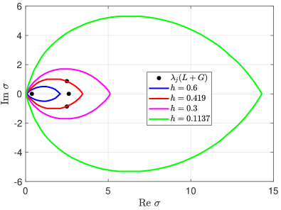
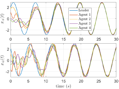
Figure 1: Left: Synchronizing regions ($\Delta_{M}$) found by Corollary 1 for various values of the delay bound $h$ for the controller $K=1.34\;[0.1\;0.6403]$. Right: State variables of the leader and agents for $\tau=0.419$ s.

Table 1: Controllers designed by the proposed approaches in Section 6 for the MAS synchronization.

Design method	$h=0.6\quad(\epsilon=0.1)$	$h=0.9\quad(\epsilon=0.1)$
Theorem 6	$K=[-0.0173\;0.2531]$	no feasible solution
Procedure 1	$\bar{K}=[-0.005\;0.2883],\quad c=1$	$\bar{K}=[-0.011\;0.1446],\quad c=1$
	$c_{min}=0.131,\quad c_{max}=1.873$	$c_{min}=0.131,\quad c_{max}=1.024$

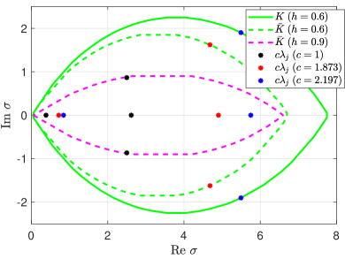
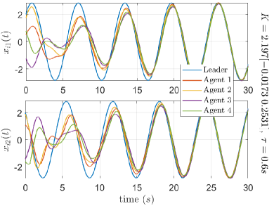
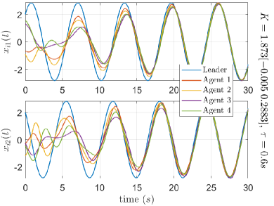
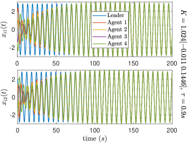
Figure 2: Upper-left: Synchronizing regions ($\Delta_{M}$) found by Corollary 1 for the control designs via Theorem 6 and Procedure 1 as in Table 1 for the upper delay bounds $h=0.6$ and $h=0.9$. Others: State variables of the leader and agents for $\tau=h$, and controllers amplified with $c_{max}$ given Table 1.

We show in Fig. 1–left the DSRs found by Corollary 1 with the resolution $\Delta=0.05$ for the proposed algorithm when $K=1.34[0.1\;0.6403]$ is chosen. Observe that $\lambda_{2,3}$ lie on the boundary of the region whereas $\lambda_{1,4}$ lies inside the region, found for the delay $h=0.419$, which is consistent with the presented result above found by Theorem 5. For comparison, note that the DSR is determined by nonlinear matrix inequalities in Hengster-Movric et al. (2015), and is not easy to determine in its entirety. Note also that the delay bound $h=0.1137$ in Hengster-Movric et al. (2015) is found for the condition $|\lambda_{max}|\leq 2.6457$. Thus, the conservatism of the DSR result is here reduced remarkably. Fig 1–right also demonstrates the synchronization of the both state variables of agents to the states of the leader when $\tau=0.419$ s in (4), where the initial state of the leader is $x_{0}(0)=[2\;2]^{T}$, and each initial state values of the agents are random values in the interval $[-2,2]$.

Let us also design the controllers proposed in Section 6 for the delay bounds $h=0.6$ and $h=0.9$. The state-feedback controllers and coupling gains are obtained for both proposed methods as in Table 1. The DSRs found by Corollary 1 and $c\lambda_{j}$ values with $c_{max}$ are illustrated in Fig 2-upperleft. It is seen that all regions contain $\forall\lambda_{j}$ and $c_{max}\lambda_{2,3}$ lie on the boundary of $\Delta_{M}$. The largest DSR is found for $K$ by means of the common LKF approach, i.e. Theorem 6, as mentioned in Remark 6. Correspondingly, $K$ can also be multiplied with any coupling gain $1\leq c\leq 2.197$, where the synchronization is still guaranteed for $h=0.6$. The other sub-figures of Fig. 2 show that the synchronization of state variables of all the agents to the leader states is achieved for all controllers multiplied by maximum coupling constants.

All the LMI problems above are solved by standard SeDuMi solver with YALMIP toolbox.

8 Concluding remarks

Synchronization of MAS with constant uniform communication and control delays is investigated. Agents are described by general LTI dynamics, and assumed to interact on a directed graph. A unified LMI approach is proposed for determining the allowable delay bound, delay-dependent synchronizing region for any given state-feedback controller, and the design of distributed cooperative state-feedback control. The proposed method is found to be less conservative both for the delay bound and synchronizing region estimates, as compared to other results existing in the literature. This is due to the LKF approach and the relaxation based on the revealed quasi-convexity property. For control design, a multiple LKF and a common LKF approach are proposed. While the multiple LKF results in a less conservative delay bound, the common LKF approach enables a more direct design and provides better robustness to graph uncertainties. For both approaches, it is sufficient to know only the upper bound on the delay and the approximate region in the complex plane where the Laplacian eigenvalues reside. Thus, those are both robust to delay and graph uncertainties.

The proposed approach can also be adapted straightforwardly to the ARE-based design of state-feedback and output feedback controllers in Li et al. (2010); Zhang, Lewis, and Das (2011). Also, it has high potential to reduce conservatism in various MAS synchronization control designs such as optimal and $H_{\infty}$ control studied in Hengster-Movric and Lewis (2014); Hengster-Movric, Lewis, and Šebek (2015). Thus, we believe this paper will have some impact on the synchronization problem of MASs without delays as well. Another potential research area is the extension of the methodology to non-uniform constant or time-varying delays. Subsequent research on the subject will follow these directions.

References

- Apkarian and Tuan (2000) Apkarian, P., and H.D. Tuan. 2000. “Parameterized LMIs in Control Theory.” SIAM Journal on Control and Optimization 38 (4): 1241–1264.
- Boyd and El Ghaoui (1993) Boyd, S., and L. El Ghaoui. 1993. “Method of centers for minimizing generalized eigenvalues.” Linear Algebra and Its Applications 188-189 (C): 63–111.
- Boyd et al. (1994) Boyd, S., L. El Ghaoui, E. Feron, and V. Balakrishnan. 1994. Linear Matrix Inequalities in System and Control Theory. Vol. 15. SIAM.
- Briat (2015) Briat, C. 2015. Linear Parameter-Varying and Time-Delay Systems Analysis, Observation, Filtering & Control. Vol. 3 of Advances in Delays and Dynamics. Springer-Verlag.
- Cao et al. (2013) Cao, Y., W. Yu, W. Ren, and G. Chen. 2013. “An overview of recent progress in the study of distributed multi-agent coordination.” IEEE Transactions on Industrial Informatics 9 (1): 427–438.
- Cepeda-Gomez and Olgac (2013) Cepeda-Gomez, R., and N. Olgac. 2013. “Exact stability analysis of second-order leaderless and leader-follower consensus protocols with rationally-independent multiple time delays.” Systems and Control Letters 62 (6): 482–495.
- Fax and Murray (2004) Fax, J.A., and R.M. Murray. 2004. “Information Flow and Cooperative Control of Vehicle Formations.” IEEE Transactions on Automatic Control 49 (9): 1465–1476.
- Fridman (2014a) Fridman, E. 2014a. Introduction to time-delay systems: Analysis and control. Systems and Control: Foundations and Applications. Birkhauser.
- Fridman (2014b) Fridman, E. 2014b. “Tutorial on Lyapunov-based methods for time-delay systems.” European Journal of Control 20 (6): 271–283.
- Fridman and Shaked (2002) Fridman, E., and U. Shaked. 2002. “An improved stabilization method for linear time-delay systems.” IEEE Transactions on Automatic Control 47 (11): 1931–1937.
- Gu (2000) Gu, K. 2000. “An integral inequality in the stability problem of time-delay systems.” In Proceedings of the IEEE Conference on Decision and Control, Vol. 3, 2805–2810.
- Gu, Kharitonov, and Chen (2003) Gu, K., V. L. Kharitonov, and J. Chen. 2003. Stability of Time-Delay Systems. Boston, MA: Birkhauser.
- Hengster-Movric and Lewis (2014) Hengster-Movric, K., and F.L. Lewis. 2014. “Cooperative optimal control for multi-agent systems on directed graph topologies.” IEEE Transactions on Automatic Control 59 (3): 769–774.
- Hengster-Movric, Lewis, and Šebek (2015) Hengster-Movric, K., F.L. Lewis, and M. Šebek. 2015. “Distributed static output-feedback control for state synchronization in networks of identical LTI systems.” Automatica 53: 282–290.