Prethermal memory loss in interacting quantum systems coupled to thermal baths

Abstract

We study the relaxation dynamics of an extended Fermi-Hubbard chain with a strong Wannier-Stark potential tilt coupled to a bath. When the system is subjected to dephasing noise, starting from a pure initial state the system’s total von Neumann entropy is found to grow monotonously. The scenario becomes rather different when the system is coupled to a thermal bath of finite temperature. Here, for sufficiently large field gradients and initial energies, the entropy peaks in time and almost reaches its largest possible value (corresponding to the maximally mixed state), long before the system relaxes to thermal equilibrium. This entropy peak signals an effective prethermal memory loss and, relative to the time where it occurs, the system is found to exhibit a simple scaling behavior in space and time. By comparing the system’s dynamics to that of a simplified model, the underlying mechanism is found to be related to the localization property of the Wannier-Stark system, which favors dissipative coupling between eigenstates that are close in energy.

The problem of particles moving in a tilted lattice (Wannier-Stark system) is associated with various interesting phenomena, such as Bloch oscillations Bloch (1929), Stark localization Wannier (1960) and Landau-Zener tunneling Zener and Fowler (1934). Despite its long history, it has kept to be a frontier research topic both theoretically Glück et al. (2002) and experimentally  Mendez et al. (1988); Pertsch et al. (1999); Morandotti et al. (1999); Wilkinson et al. (1996); Ben Dahan et al. (1996); Morsch et al. (2001); Kling et al. (2010); Trompeter et al. (2006); Dreisow et al. (2009); Mukherjee et al. (2015); Schmidt et al. (2018a); Guardado-Sanchez et al. (2019). Recent studies van Nieuwenburg et al. (2019); Schulz et al. (2019) show that an interacting Wannier-Stark system can exhibit non-ergodic behavior analogous to disorder-induced many-body localization (MBL) Altman and Vosk (2015); Nandkishore and Huse (2015); Alet and Laflorencie (2018); Abanin et al. (2019). Understanding both the differences and similarities between such disorder-free and conventional MBL constitutes a fundamental question, which currently attracts a lot of attention Khemani et al. (2019); Sun et al. (2019); Taylor et al. (2019); Brenes et al. (2018); Smith et al. (2017a); Grover and Fisher (2014); Schiulaz et al. (2015); Yao et al. (2016); Papić et al. (2015); Smith et al. (2017b, a); De Roeck and Huveneers (2014); Hickey et al. (2016); van Horssen et al. (2015); Carleo et al. (2012).

On the other hand, there is an increased recent interest in the non-equilibrium properties of open many-body quantum systems Breuer and Petruccione (2002); Carmichael (2013); Pichler et al. (2010); Daley (2014); Garrahan and Lesanovsky (2010); Diehl et al. (2008); Verstraete et al. (2009); de Vega and Alonso (2017); Vorberg et al. (2013, 2015); Schnell et al. (2017); Poletti et al. (2012); Bernier et al. (2018); Baumann et al. (2010); Ritsch et al. (2013); Ludwig and Marquardt (2013); Ashida et al. (2018); Nakagawa et al. (2019); Deffner and Lutz (2011); Labouvie et al. (2016); Lüschen et al. (2017); Wu et al. (2019); Wu and Eckardt (2019); Levi et al. (2016); Fischer et al. (2016); Medvedyeva et al. (2016); Everest et al. (2017); Žnidarič et al. (2016); Nissen et al. (2012); Marcuzzi et al. (2014); Tamascelli et al. (2019); Xu et al. (2019); Wang et al. (2014). While the coupling to an environment of finite temperature constitutes a natural situation, it is rather cumbersome to simulate. Therefore, the impact of dissipation is often treated by using dephasing noise Gardiner et al. (2004) as a simpler bath model. Even though dephasing noise will eventually drive the system into an infinite-temperature state, it is assumed to qualitatively capture the effect of weak coupling to a bath on the transient evolution. Understanding, under which circumstances this assumption breaks down is an important question for the simulation of open many-body systems (see also Refs. Guo et al. (2018); Tan et al. (2019)).

Here we report on a surprising phenomenon in the relaxation dynamics of an interacting Wannier-Stark system coupled to a thermal bath of finite temperature. It sheds light on both of the above questions, since it can neither be observed for a disorder-localized system nor for dephasing noise. In a large parameter regime, we find that long before the system reaches thermal equilibrium, it transiently approaches the maximally mixed state. This effect implies an effective prethermal memory loss. It is reminiscent of the universal dynamics recently observed in isolated quantum gases Prüfer et al. (2018); Erne et al. (2018).

We consider a one-dimensional extended Hubbard chain half filled with spin-polarized fermions and subjected to a linear potential gradient. It is described by the Hamiltonian

Here $c_{i}^{\dagger}$ and $n_{i}=c^{\dagger}_{i}c_{i}$ are the creation and number operator for a fermion on lattice site $i$. Moreover, $J$ is the tunneling parameter, $W_{i}=-ri$ captures the potential gradient $r$, and $V$ quantifies nearest-neighbor interactions. The single-particle (bulk) eigenstates, known as Wannier-Stark states, are centered at the lattice sites, with a localization length $\sim J/2r$ (with respect to the site index $i$) and energies that increase by $r$ from site to site Wannier (1960). Moreover, also the interacting system shows properties akin to MBL van Nieuwenburg et al. (2019); Schulz et al. (2019). Henceforth, we use $J$, $J/k_{B}$, and $\hbar/J$ as units for energy, temperature, and time, respectively, so that $J=\hbar=k_{B}=1$.

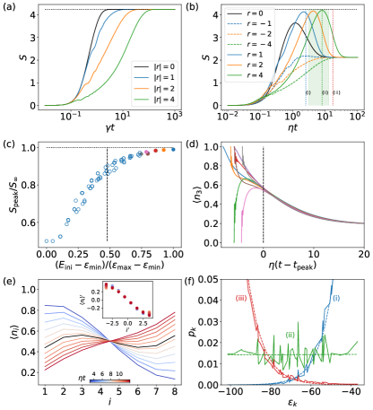
Figure 1: (a), (b) Time evolution of the von Neumann entropy for the tilted ladder (1) initialized in a Fock state with the left half of the chain occupied and coupled to (a) a dephasing bath [Eq. (3)] or (b) a thermal bath [Eq. (Prethermal memory loss in interacting quantum systems coupled to thermal baths)]. The dotted line marks the largest possible entropy $S_{\infty}$. (c) Normalized peak entropy for initial Fock states of various energies $E_{\text{ini}}$. The vertical dashed line marks $E_{\infty}$. (d) Evolution of the mean occupation of the third lattice site relative to the time $t_{\text{peak}}$, where the entropy peak is reached. The line colors mark different initial Fock states corresponding to colored bullets in (c). (e) Density profile $\langle n_{i}\rangle$ at equidistant times during the time window marked by the shaded area in (b). The black line marks $t=t_{\text{peak}}$. The inset shows the collapse of all the curves by rotating them by an angle proportional to the corresponding time. (f) Diagonal elements of the density matrix $p_{k}$ at three points in time [marked by (i)-(iii) in (b)] (solid lines) compared to effective thermal states of identical average energy (dashed lines). The parameters are $M=8$, $V=1$, $\gamma=\eta=0.1$, and $T$ so that $S_{T}=S_{\infty}/2$. The field gradient for (c)-(f) is $r=4$.

When coupled weakly to a thermal bath, which is modeled as a collection of harmonic oscillators in thermal equilibrium and couples to the on-site occupations, the system can be described by a Redfield master equation Breuer and Petruccione (2002),

$$\frac{d\rho}{dt}= -i\left[H,\rho\right]+\eta\sum\limits_{k,q,p,l=1}^{M}{}\left[{R_{kqlp}\left(L_{kq}\rho L_{pl}^{\dagger}-L_{pl}^{\dagger}L_{kq}\rho\right)}\right.$$

$$+\left.{R_{plqk}\left(L_{kq}\rho L_{pl}^{\dagger}-\rho L_{pl}^{\dagger}L_{kq}\right)}\right],$$ (2)

with jump operators $L_{kq}=|k\rangle\langle q|$ between many-body eigenstates $|k\rangle$ of energy $\varepsilon_{k}$ Vorberg et al. (2015); Wu et al. (2019). The corresponding transition rates read $R_{kqpl}=\pi v_{kqpl}g({\varepsilon}_{k}-{\varepsilon}_{q})$, with $v_{kqpl}=\sum\limits_{i=1}^{M}{\langle k|n_{i}|q\rangle\langle p|n_{i}|l\rangle}$ and bath correlation function $g(E)=J(E)/(e^{E/T}-1)$, where we assume an Ohmic spectral density $J(E)=E$.

In the high-temperature limit, we have $g(E)\simeq T$ and the transition rate $R_{kqpl}$ becomes independent of energy. Thus, the master equation reduces to

$$\frac{d\rho}{dt}=-i\left[H,\rho\right]+\gamma\sum\limits_{i=1}^{M}{\left(n_{i}\rho n_{i}-\frac{1}{2}n_{i}^{2}\rho-\frac{1}{2}\rho n_{i}^{2}\right)},$$ (3)

with $\gamma=\eta T$, describing dephasing noise.

Figure 1 shows the time evolution of the von Neumann entropy $S=-\mathrm{tr}\{\rho\log(\rho)\}$ of the total system, when coupled to (a) a dephasing bath or (b) a finite-temperature bath. It is calculated by numerically integrating Eqs. (3) and (Prethermal memory loss in interacting quantum systems coupled to thermal baths), respectively, starting from a Fock state with the left half of the chain occupied. The temperature $T$ of the thermal bath is chosen such that the corresponding equilibrium entropy, $S_{T}$ (obtained for the Gibbs state $\rho_{T}={\cal Z}_{T}^{-1}\sum_{k}e^{-\varepsilon_{k}/T}|k\rangle\langle k|$ with ${\cal Z}_{T}=\sum_{k}e^{-\varepsilon_{k}/T}$), is equal to half the largest possible entropy $S_{\infty}\equiv S_{T=\infty}=\log({\cal D})$, with Hilbert space dimension ${\cal D}=M!/[(M/2)!]^{2}$ (see Fig. S1 of Ref. sm for other temperatures). For dephasing noise [Fig. 1(a)], the entropy grows monotonously to the maximum value $S_{\infty}$, being insensitive to the sign of the potential gradient $r$. In turn, when the system is coupled to the finite- temperature bath [Fig. 1(b)], the entropy approaches its equilibrium value rather differently for negative and positive $r$. While in the former case the entropy grows monotonously to $S_{T}$ (except for small $|r|$), in the latter case it first reaches a peak value $S_{\text{peak}}$ well above $S_{T}$, before relaxing to equilibrium. As will become apparent in the following, this difference can be attributed to the different mean energies of the initial states.

Remarkably, we can observe in Fig. 1(b) that for large positive gradients $r$, the peak entropy almost reaches the largest possible entropy $S_{\infty}$ (dotted line), which uniquely corresponds to the maximally mixed state $\rho_{\infty}\equiv\rho_{T=\infty}=\mathcal{D}^{-1}\sum_{k}|k\rangle\langle k|$. This effect can be observed for a wide range of initial conditions: In Fig. 1(c) we plot the peak entropies $S_{\text{peak}}$ reached during the evolution starting from various initial Fock states, versus their mean energy $E_{\text{ini}}$ (scaled between 0, for the ground-state energy $\varepsilon_{\text{min}}$, and 1, for the energy $\varepsilon_{\text{max}}$ of the most excited state). Peak entropies close to $S_{\infty}$ are found as long as $E_{\text{ini}}$ lies well above the energy $E_{\infty}=\mathrm{tr}\{\rho_{\infty}H\}$ of the maximally mixed state (dashed line).

Since the maximally mixed state is unique, reaching an entropy peak with $S_{\text{peak}}\approx S_{\infty}$ indicates that we can expect the system dynamics to become (approximately) independent of the initial conditions near and after approaching the peak entropy. Such a behavior is confirmed in Fig. 1(d), where we plot the evolution of the site occupation $\langle n_{i=3}\rangle$ relative to the time $t_{\text{peak}}$ at which the entropy peak is reached. The different curves, which correspond to different initial states [labeled by line colors corresponding to the colored bullets in Fig. 1(c)], clearly converge near $\eta(t-t_{\text{peak}})=0$ and subsequently show almost identical behavior. Similar behavior can also be observed for other site occupations $\langle n_{i}\rangle$ and for larger systems (see Figs. S3, S4 and Figs. S6, S9 of Ref. sm , respectively). Thus, the system undergoes an effective prethermal memory loss, long before it reaches thermal equilibrium.

Moreover, we also find that the way the system approaches the maximally mixed state shows a simple form of scaling behavior. In Fig. 1(e) we plot the density distribution, $\langle n_{i}\rangle$, at various times near $t_{\text{peak}}$ [within the shaded area in Fig. 1(b)], for $r=4$ and starting from the Fock state with the left half of the chain occupied [green curve in Fig. 1(b)]. These density profiles collapse on top of each other when rotated by an angle proportional to the evolved time (see inset). Note that for $r=4$ the Wannier-Stark states are already well localized on single lattice sites, so that the plotted density profile (which can directly be measured in quantum-gas systems) approximately corresponds to the occupation of the single-particle eigenstates. In this sense, the observed behavior is somewhat reminiscent of the universal scaling behavior recently observed in the occupations of long-wavelengths momentum modes during the far-from equilibrium dynamics of isolated quantum gases Prüfer et al. (2018); Erne et al. (2018), which was associated with the presence of non-thermal fixed points Berges et al. (2008); Piñeiro Orioli et al. (2015); Nowak et al. (2011).

Further insight on how the system approaches the maximally mixed state is gained by looking at the probability distribution $p_{k}=\langle k|\rho|k\rangle$ for occupying many-body energy eigenstates $|k\rangle$. In Fig. 1(f) we plot the distribution $p_{k}$ (solid lines) for $r=4$ at three times: (i) slightly before, (ii) at, and (iii) slightly after $t_{\text{peak}}$ [as indicated in Fig. 1(b) relative to the green curve]. Interestingly, these distributions agree rather well to those for thermal states $\rho_{T_{\text{eff}}}$ (dashed lines) with the effective temperature $T_{\text{eff}}$ determined by the instantaneous energy, $\mathrm{tr}\{\rho_{T_{\text{eff}}}H\}\equiv E=\mathrm{tr}\{\rho H\}$. This observation suggests that the prethermal memory loss is due to a dissipative form of prethermalization, where the system rapidly approaches a Gibbs state, whose effective temperature $T_{\text{eff}}$ then slowly relaxes to the equilibrium temperature $T$. This scenario immediately explains that an infinite temperature state is approached long before the system has thermalized as long as the initial energy $E_{\text{ini}}$ lies well above the infinite-temperature energy $E_{\infty}$. Namely, in this case the system has enough time to approach a prethermal state $\rho_{T_{\text{eff}}}$, before $1/T_{\text{eff}}$ passes through zero from below at the time when $E$ drops below $E_{\infty}$.

The prethermal relaxation to a Gibbs-like state with slowly varying effective temperature occurs in a way rather different from standard (pre)thermalization Berges et al. (2004). It cannot be understood as the prethermalization of system and bath together, since the bath always remains in the same thermal state with constant temperature $T$. Nor can it be explained by the thermalization of the system itself on a time scale that is fast compared to slow energy dissipation by the bath, since the system is localized and non-ergodic. Let us, therefore, investigate the underlying mechanism and its relation to Stark localization.

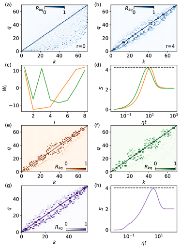
Figure 2: (a), (b) Rate matrix for the Fermi-Hubbard chain coupled to a thermal bath, with $r=0$ (a) and $r=4$ (b). (c) Examples for on-site potentials $W_{i}$ that were optimized over the range $[-16,16]$ to provide a large peak entropy when evolving from the most excited state. The results are representative for $500$ numerical runs. (d) Time evolution of the corresponding entropies. (e)-(f) Corresponding rate matrices $R_{kq}$. (g) Rate matrix and (h) entropy for a tilted bosonic Hubbard chain with $r=4$ and initially all particles occupying the leftmost site. The system sizes are $M=8$, $N=4$ for (a)-(f), and $M=6$, $N=3$ for (g)-(h). Other parameters are $V=1$, $\eta=0.1$, and $T$ so that $S_{T}=S_{\infty}/2$.

Although a two-level system prepared in its excited state passes through the maximum entropy state while equilibrating with a thermal bath sm , such behavior is highly nontrivial for interacting many-body systems. To figure out the conditions for a close-to-maximum peak entropy, let us focus on the weak-coupling limit, where the secular approximation Breuer and Petruccione (2002); Carmichael (2013) gives a Lindblad master equation,

$$\frac{d\rho}{dt}=-i\left[H,\rho\right]+\eta\sum\limits_{k,q=1}^{M}{}R_{kq}{\left(L_{kq}\rho L_{kq}^{\dagger}-\frac{1}{2}\left\{L_{kq}^{\dagger}L_{kq},\rho\right\}\right)},$$

with rates $R_{kq}\equiv R_{kqqk}$. They obey $R_{kq}/R_{qk}=e^{-(\varepsilon_{k}-\varepsilon_{q})/T}$, so that low energy states are favored and the system is asymptotically driven towards the Gibbs state $\rho_{T}$. The matrix elements $\rho_{kq}\equiv\langle k|\rho|q\rangle$ follow $\dot{\rho}_{kq}=-i({\varepsilon}_{k}-{\varepsilon}_{q})\rho_{kq}+\eta\sum_{p}{\left[R_{kp}\rho_{pp}\delta_{kq}-\frac{1}{2}(R_{pk}+R_{pq})\rho_{kq}\right]}$, where diagonal and off-diagonal elements decouple from each other. The latter decay with rates $\Gamma_{kq}=\frac{1}{2}\eta\sum_{p}{(R_{pk}+R_{pq})}$ and have to be negligible already when the peak entropy is reached, to allow for the observed transient approach of the maximally mixed state (this is indeed the case, see Fig. S2 and discussion in Ref. sm ). The dynamics of the diagonal elements $p_{k}\equiv\rho_{kk}$ is determined by the rate matrix $R_{kq}$ through the Pauli rate equation $\dot{p}_{k}=\eta\sum_{q}{\left[R_{kq}p_{q}-R_{qk}p_{k}\right]}$ Breuer and Petruccione (2002).

In Fig. 2 (a) and (b) we compare rate matrices for $r=0$ and $r=4$. Without potential gradient, one finds long-range coupling with respect to energy. In contrast, at a large field gradient ($r=4$) the transition rates predominantly couple states that are close by in energy. The latter is a consequence of Stark localization, where eigenstates that are close in space, so that they are coupled by the bath via the densities $n_{i}$, are close also with respect to energy. Note that for a disorder-localized Fermi-Hubbard chain without this spatio-energetic correlation we find non-local rate matrices and no prethermal memory loss (see Fig. S10 of Ref. sm ). This constitutes an even more drastic difference between the relaxation dynamics of Stark and disorder-induced MBL than the one observed for dephasing noise Wu and Eckardt (2019).

To check, whether a rate matrix with energy-local coupling is crucial for the appearance of a close-to-maximum entropy ($S_{\rm peak}\simeq S_{\infty}$), we investigate the rate matrices for rather different on-site potentials $W_{i}$ [see Fig. 2(c)] that (were optimized to) equally give rise to large peak entropies [see Fig. 2(d)]. It turns out that, indeed, they also show near-neighbor coupling [see Figs. 2(e)-(f)]. Moreover, also the tilted bosonic Hubbard chain [given by Eq. (1) with bosonic annihilation operators $c_{i}$ and the last term replaced by on-site interactions $\frac{1}{2}V\sum_{i}n_{i}(n_{i}-1)$] shows $S_{\text{peak}}\approx S_{\infty}$ together with an energy local rate matrix [see Figs. 2(g)-(h)]. This, together with results for simplified models shown below (and in Fig. S13 of Ref. sm ) indicates clearly that the prethermal memory loss discussed here is a very robust phenomenon.

To address the question, why the appearance of a close-to-maximum entropy is associated with local coupling between energy states, let us now consider a simplified rate model. Here the energy eigenstates have equally spaced non-degenerate energies $\varepsilon_{k}=rk$, with $k=0,1,\cdots\mathcal{D}-1$, and are coupled by thermal rates that are homogeneous and local with respect to energy. We define $R_{k+n,k}\equiv R_{n}$, where $R_{n}=0$ for $|n|>n_{m}$ and $R_{n}=g(nr)$ for $|n|\leq n_{m}$, so that (as a property of the bath correlation function $g$) $R_{n}/R_{-n}=(R_{+}/R_{-})^{n}=e^{-nr/T}$, with $R_{\pm}\equiv R_{\pm 1}$.

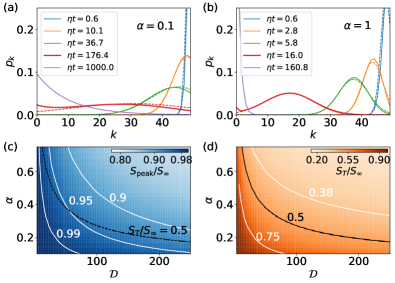
Figure 3: Simplified rate model with nearest-neighbor coupling $n_{m}=1$ evolving from most escited state. (a), (b) Probability distribution $p_{k}$ at different times for $\mathcal{D}=50$ and $\alpha=0.1$ (a) and 1 (b). (c), (d) Normalized peak and thermal entropies $S_{\text{peak}}/S_{\infty}$ (c) and $S_{\rm T}/S_{\infty}$ (d) versus $\alpha$ and ${\cal D}$.

Let us first study nearest-neighbor coupling, $n_{m}=1$. By defining $\nabla^{2}p_{k}=p_{k+1}+p_{k-1}-2p_{k}$ and $\nabla p_{k}=(p_{k+1}-p_{k-1})/2$, we can write the Pauli rate equation as a discrete drift-diffusion equation, $\dot{p}_{k}=\eta(\bar{R}\nabla^{2}p_{k}+\delta R\nabla p_{k})$ Chandrasekhar (1943), where diffusion and drift are quantified by $\bar{R}\equiv(R_{+}+R_{-})/2$ and $\delta R\equiv R_{-}-R_{+}$, respectively. Scaling time with $(\eta\bar{R})^{-1}$, the model is completely characterized by the ratio $\alpha=\delta R/{\bar{R}}$ and the system size $\mathcal{D}$. Starting from the highest excited state, $p_{k}(0)=\delta_{k,k_{\text{ini}}}$ with $k_{\text{ini}}=\mathcal{D}-1$, and setting $\mathcal{D}=50$, in Figs. 3(a) and (b) we plot $p_{k}$ for $\alpha=0.1$ and $\alpha=1$ for different times (solid lines, fat red lines indicate $t_{\text{peak}}$). While for $\alpha=0.1$, a rather uniform distribution is found at a time $t_{\text{peak}}$, approximating the maximum entropy state with $p_{k}=1/\mathcal{D}$, this is not the case for larger drift, $\alpha=1$. Before reaching thermal equilibrium, we find the distribution well approximated by a Gaussian of standard deviation $\sigma=\sqrt{2{\bar{R}}t}$ centered at $k_{0}=k_{\text{ini}}-\delta Rt$ Chandrasekhar (1943) (dashed lines). The condition for reaching an almost flat distribution is, thus, given by the intuitive requirement that the drift time needed to reach $k_{0}=\mathcal{D}/2$, $\tau_{F}=(k_{\text{ini}}-\mathcal{D}/2)/\delta R$, is larger than the diffusion time giving rise to $\sigma=\mathcal{D}/2$, $\tau_{D}=\mathcal{D}^{2}/(8{\bar{R}})$. Thus, for $k_{\text{ini}}=\mathcal{D}-1$ we expect $S_{\text{peak}}\approx S_{\infty}$ as long as $\alpha\lesssim 4\mathcal{D}^{-1}$, which is confirmed in Fig. 3(c) [see also Fig. S12(a) of Ref. sm ].

However, $S_{\text{peak}}\approx S_{\infty}$ is a non-trivial result only as long as the thermal entropy $S_{T}$, plotted in Fig. 3(d), lies well below $S_{\infty}$. For $\mathcal{D}r\gg T$ we can neglect the upper bound of the spectrum and $S_{T}$ approaches the value for an harmonic oscillator with frequency $r$ Gould and Tobochnik (2010), $S_{T}\simeq\frac{x}{x-1}\log(x)-\log(1-x)$ with $x=e^{-r/T}=R_{+}/R_{-}=(2-\alpha)/(2+\alpha)$, so that for $\alpha\ll 1$ one has $S_{T}\simeq\log(1/\alpha)+1+\mathcal{O}(\alpha)$ [Fig. 3(d)]. Thus, $S_{T}/S_{\infty}<s$ as long as $\alpha\gtrsim e\mathcal{D}^{-s}$. While for $\mathcal{D}\to\infty$ this requirement is incompatible with the one for large peak entropies, $\alpha\lesssim 4\mathcal{D}^{-1}$, it turns out that the different prefactors appearing in both conditions (whose values can deviate from our estimates $e$ and $4$) still give rise to a large non-trivial regime for finite $\mathcal{D}$, as can be inferred from Figs. 3(c) and (d).

The simplified rate model with $n_{m}=1$ roughly corresponds to the case of a single particle in a tilted lattice. While it describes peak entropies $S_{\text{peak}}\approx S_{\infty}$ and prethermal memory loss, it gives rise to a Gaussian rather than an exponential prethermal distribution. This suggests that the formation of a prethermal Gibbs state requires more complex rate matrices as they are found for the many-particle case. In Fig. 4 we investigate, what happens when increasing the coupling range $n_{m}$, and thus the complexity, of the simplified rate model [using $\mathcal{D}=50$ and $\eta=0.1$]. We observe that $S_{\text{peak}}$ first increases with $n_{m}$ before, after reaching a maximum at $n_{m}=11$, it decreases again. The first increase with $n_{m}$ might be explained by the prethermal distribution becoming more Gibbs like and thus flatter at $t=t_{\text{peak}}$ than the Gaussian (which always retains a finite $\sigma$). This is confirmed in Fig. 4(b), where we plot the distribution $p_{k}$ at different times for $n_{m}=11$ and find rather good agreement with an effective Gibbs state. The subsequent decrease of $S_{\text{peak}}$ can, in turn, be attributed to an increase of the drift velocity with $n_{m}$, which is clearly visible also in Fig. 4(a) and which reduces the time available for reaching a prethermal distribution. This mechanism explains, why large transient peak entropies $S_{\text{peak}}\approx S_{\infty}$, are found for rate matrices that are local in energy.

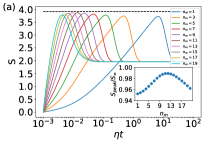
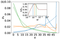
Figure 4: Evolution of the simplified rate model starting from the most excited state for $\mathcal{D}=50$, $\eta=0.1$, and $T$ so that $S_{T}=S_{\infty}/2$. (a) Entropy evolution for different $n_{m}$. Inset: Normalized peak entropies versus $n_{m}$. (b) Distribution $p_{k}$ (solid lines) for $n_{m}=11$ at the times marked in the inset compared to effective Gibbs states (dashed lines).

In conclusion, we have shown that the non-equilibrium relaxation dynamics of interacting Wannier-Stark ladders coupled to a finite-temperature environment can feature effective prethermal memory loss. The effect is found to rely on a dissipative form of prethermalization. In experiment with ultracold atoms, a thermal environment could be provided, for instance, by the coupling to a second atomic species Schmidt et al. (2018b).

A two-level system

Consider a two-level system with eigenstates $|+\rangle$, $|-\rangle$ and the corresponding eigenenergies ${\varepsilon}_{\pm}$. According to the Lindblad master equation introduced in the main text, the dynamics of the corresponding occupation probabilities $p_{\pm}$ is governed by the Pauli master equation

$$\dot{p}_{+}=\eta(R_{+-}p_{-}-R_{-+}p_{+})=-\dot{p}_{-}.$$ (S1)

Its solution is given by

$$p_{+}=\alpha-(\alpha-p_{+}(0))e^{-\eta R_{0}t}=1-p_{-},$$ (S2)

where $R_{0}=R_{+-}+R_{-+}$ and $\alpha=R_{+-}/R_{0}$. While $\alpha=1/2$ for dephasing noise, for a thermal bath of finite temperature we find $\alpha=\left(1+e^{2\Omega/T}\right)^{-1}$, with $\Omega={\varepsilon}_{+}-{\varepsilon}_{-}$ being the energy splitting.

The off-diagonal terms of the density matrix

$$\rho=\begin{pmatrix}p_{+}&\rho_{+-}\\ \rho_{-+}&1-p_{+}\end{pmatrix},$$ (S3)

are described by

$$\rho_{\pm\mp}=e^{\mp i\Omega t-\eta R_{s}t/2}\rho_{\pm\mp}(0),$$ (S4)

with $R_{s}=\sum_{k,q=\pm}R_{kq}$.

To quantify the difference between thermal bath and dephasing noise, we investigate the purity. It is calculated as $f=\sum_{k}\lambda_{k}^{2}$, with $\lambda_{k}$ being the eigenvalues of the density matrix. It shows similar behavior as the von Neumann entropy $S=-\sum_{k}{\lambda_{k}\log(\lambda_{k})}$, but is easier to handle analytically. For the two-level system, we can verify that the purity is given by

$$f = {\frac{1}{2}+2|\rho_{+-}|^{2}+2\left(p_{+}-1/2\right)^{2}}$$ (S5)

$$= A_{1}e^{-\eta R_{0}t}+A_{2}e^{-2\eta R_{0}t}+Be^{-\eta R_{s}t}+C,$$

with

$$A_{1} = 2(1-2\alpha)(\alpha-p_{+}(0)),$$

$$A_{2} = 2(\alpha-p_{+}(0))^{2},$$

$$B = 2|\rho_{+-}(0)|^{2},$$

$$C = 2\alpha(\alpha-1)+1.$$ (S6)

Except for $A_{1}$, all the other coefficients are non-negative. For dephasing noise, we have $\alpha=1/2$, thus $A_{1}=0$. Hence, the purity $f$ decays monotonously to its steady state value $C=1/2$. While for a finite-temperature bath, $A_{1}$ can be negative, depending on the parameters of the system and the initial state. When $A_{1}<0$, there will be a competition between the first term and the others, leading to a non-monotonous behavior in the purity. An obvious example is when we start from the excited state. Then the purity will degrade from its initial value $1$ (for a pure state with $p_{+}=1$) to the minimal value $1/2$ (uniquely corresponding to the maximally mixed state with $p_{+}=p_{-}=1/2$), and then increase again until it approaches the steady state value (for the finite-temperate thermal state with $p_{+}<1/2$). In contrast, if the initial state is the ground state, the purity decreases monotonously, both for thermal bath and dephasing noise.

1D spinless Fermion chain subjected to a linear potential

.1 Dependence of the entropy on temperature

Figure S1(a) shows the dynamics of the von Neumann entropy $S$ for a half-filling spinless Fermion chain described by Hamiltonian (1) in the main text coupled to a thermal bath at different temperatures. The peak entropy during the evolution shows a weak dependence on the temperature, with a larger entropy at a higher temperature, as shown in Fig. S1(b).

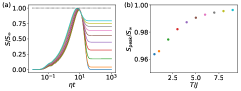
Figure S1: (a) Time evolution of the von Neumann entropy $S$ for a half-filling spinless Fermion chain whose dynamics is governed by Eq. (Prethermal memory loss in interacting quantum systems coupled to thermal baths). The dotted line marks the maximum entropy $S_{\infty}$ for the maximally mixed state. The initial state is a Fock state with the left side of the chain occupied. (b) Peak entropy $S_{\rm peak}$ as a function of the temperature of the thermal bath. The parameters are $M=8$, $V=J$, $r=4J$, $\eta=0.1J$.

.2 Dependence of the entropy on the initial state

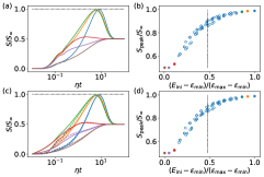
Figure S2: (a),(c) Time evolution of the von Neumann entropy $S$ for a half-filling spinless Fermion chain coupled to a thermal bath described by Eq. (Prethermal memory loss in interacting quantum systems coupled to thermal baths). The dotted line marks the maximum entropy $S_{\infty}$ for the maximally mixed state. The temperature of the thermal bath is chosen such that $S_{T}=S_{\infty}/2$. (b),(d) Peak entropy $S_{\rm peak}$ (normalized by $S_{\infty}$) as a function of the averaged energy of the initial state $E_{\rm ini}$ (scaled between 0, for the ground-state energy $\varepsilon_{\text{min}}$, and 1, for the energy $\varepsilon_{\text{max}}$ of the most excited state). The dotted line marks the average energy of the system, which is also the mean energy of the maximally mixed state (infinity-temperature state), $E_{\infty}=\mathrm{tr}\{\rho_{\infty}H\}$. The initial states for (a), (b) are Fock states, and the initial states for (c), (d) are many-body energy eigenstates. The dashed lines in (c) are the results of (a). The parameters are $M=8$, $V=J$, $r=4J$, $\eta=0.1J$.

In Fig. S2 we compare the time evolution of the entropy for different initial states. While (a) and (b) correspond to initial Fock states, (c) and (d) capture the dynamics starting from many-body energy eigenstates. While for the former scenario the initial density matrix possesses off-diagonal elements in energy representation, this is not the case the for tlatter one. Thus, the fact that both scenarios show almost identical behavior, indicates that the off-diagonal elements of the initial Fock states have decayed before reaching the peak entropy.

.3 Universal behavior of mean occupation in real space

Figure S3 shows time evolution of the mean occupation in real space $\langle n_{i}\rangle$ for a half-filling chain under a linear potential described by Hamiltonian (1) starting from different initial Fock states. The dashed lines denote the time $t_{\rm peak}$ when the peak entropy is reached. By plotting the evolution of the site occupation relative to the time $t_{\rm peak}$, the different curves clearly converge near $t=t_{\rm peak}$, as shown in Fig. S4.

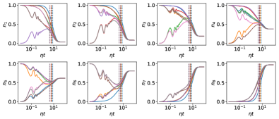
Figure S3: Time evolution of the mean occupation in real space $\langle n_{i}\rangle$ for a half-filling Fermion chain [with Hamiltonian (1)] coupled to a thermal bath described by Eq. (Prethermal memory loss in interacting quantum systems coupled to thermal baths). The vertical dashed lines marks the time when the entropy gets maximal. The initial states are $7$ Fock states with the highest energies. The parameters are $M=8$, $r=4J$, $V=J$, $\eta=0.1J$.

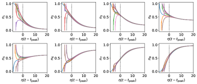
Figure S4: The same as Fig. S3 except that the time $t$ is shifted by the time to get the peak entropy $t_{\rm peak}$. The black dashed line marks $t=t_{\rm peak}$.

In Fig. S5, we show the mean occupation in real space starting from three different initial Fock states [(b)-(d)] for the time window marked by shading area in (a). The density profiles at different times in the vicinity of peak entropy are found to share similar shape. As shown in the inset, by rotating these curves by an angle proportional to the corresponding time, they collapse onto each other.

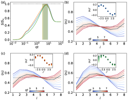
Figure S5: (a) Time evolution of the von Neumann entropy $S$ for a half-filling spinless Fermion chain [with Hamiltonian (1)] coupled to a thermal bath described by Eq. (Prethermal memory loss in interacting quantum systems coupled to thermal baths) starting from three different initial Fock states. (b)-(d) Mean occupation in real space for the time window marked by shading area in (a). The inset shows the collapse of the curves by rotating them by an angle proportional to the corresponding time. The axis in the inset is $i^{\prime}=(i-i_{0})\cos[\chi(t-t_{0})]+(\langle n_{i}\rangle-y_{0})\sin[\chi(t-t_{0})]$, and $\langle n_{i}\rangle^{\prime}=(\langle n_{i}\rangle-y_{0})\cos[\chi(t-t_{0})]-(i-i_{0})\sin[\chi(t-t_{0})]$ with the parameters $x_{0}$, $y_{0}$, $t_{0}$ and $\chi$ adjusted to get the optimal collapse. The parameters are $M=8$, $V=J$, $r=4J$, $\eta=0.1J$, $T$ is chosen to make $S_{T}=S_{\infty}/2$.

.4 Results for larger systems

.4.1 Pauli rate equation

According to the Lindblad master equation introduced in the main text, the dynamics of the diagonal and off-diagonal elements of the density matrix are decoupled. By neglecting the off-diagonal elements (which allows us to study larger system), the density matrix is given by $\rho=\sum_{k}p_{k}|k\rangle\langle k|$, with the diagonal elements $p_{k}$ governed by the Pauli rate equation

$${\dot{p}_{k}}=\eta\sum_{q}{\left({{R_{kq}}{p_{q}}-{R_{qk}}{p_{k}}}\right)}.$$ (S7)

Figure S6 shows time evolution of the mean occupation in real space $\langle n_{i}\rangle$ for a half-filling Fermion chain with $M=16$ sites by solving Eq. (S7). We find similar universal dynamics as in small system [see Fig. S4].

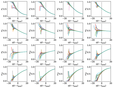
Figure S6: Time evolution of the mean occupation in real space $\langle n_{i}\rangle$ starting from different initial states with high energies. The density matrix is approximated by $\rho=\sum_{k}p_{k}|k\rangle\langle k|$ with $p_{k}$ governed by Eq. (S7). The parameters are $M=16$, $V=J$, $r=4J$.

.4.2 Kinetic theory

The equations of motion for the mean occupations in single-particle eigenstates are given by

$$\langle{\dot{n}}_{k}\rangle=\sum_{q}{\left[{\tilde{R}}_{kq}\langle(1-n_{k})n_{q}\rangle-{\tilde{R}}_{qk}\langle(1-n_{q})n_{k}\rangle\right]},$$ (S8)

where ${\tilde{R}}_{kq}=\sum_{i}|\psi_{ik}|^{2}|\psi_{iq}|^{2}$ and $\psi_{iq}$ is the single particle eigenstate. In order to obtain a closed set of equations in terms of the mean occupations, we employ the mean-field approximation,

$$\langle n_{k}n_{q}\rangle\simeq\langle n_{k}\rangle\langle n_{q}\rangle,$$ (S9)

for $k\neq q$. Then we obtain a set of nonlinear kinetic equations of motion

$$\langle{\dot{n}}_{k}\rangle=\sum_{q}{\left[\left({\tilde{R}}_{kq}\langle n_{q}\rangle-{\tilde{R}}_{qk}\langle n_{k}\rangle\right)-\left({\tilde{R}}_{kq}-{\tilde{R}}_{qk}\right)\langle n_{k}\rangle\langle n_{q}\rangle\right]},$$ (S10)

which can be solved numerically.

The mean-field approximation is equivalent to a Gaussian ansatz for the density matrix

$$\rho=\frac{1}{\cal Z}\exp(-\sum_{k}\alpha_{k}n_{k}),$$ (S11)

where ${\cal Z}$ is the partition function and $\alpha_{k}$ is determined by the $M$ mean occupations $\langle n_{k}\rangle$, as $\alpha_{k}=\ln(\langle n_{k}\rangle^{-1}-1)$. Figure S7 compares the time evolution of entropy for a half-filling chain of $M=8$ sites from exact diagonalization (solid lines) and from mean-field theory (dashed lines) for different initial Fock states. Figure S8 compares the time evolution of the corresponding mean occupation in real space. The deviations that are visible in the steady state result from the fact that Eq. (S11) corresponds to the grand canonical ensemble, rather than to a canonical Gibbs state. Figure S9 shows the time evolution of the mean occupation in real space for a half-filling chain of $M=20$ sites from mean-field theory starting from different initial Fock states.

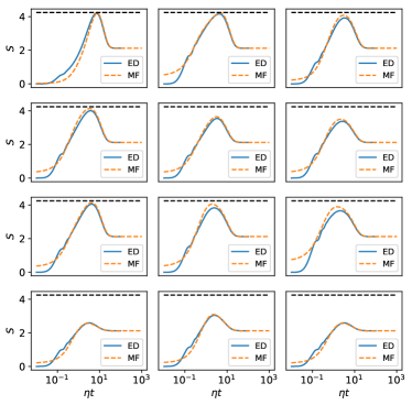
Figure S7: Comparison of time evolution of entropy from numerically solving Eq. (Prethermal memory loss in interacting quantum systems coupled to thermal baths) (solid lines) and from kinetic theory (dashed lines) for different initial Fock states. The parameters are $M=8$, $V=0$, $r=4J$.

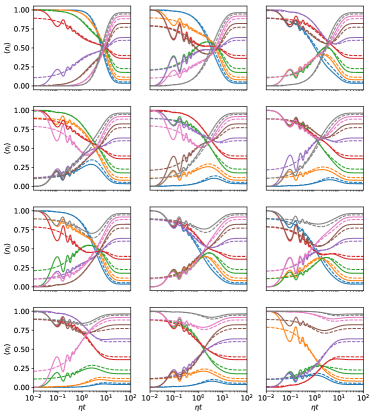
Figure S8: Comparison of time evolution of the mean occupation in real space $\langle n_{i}\rangle$ from numerically solving Eq. (Prethermal memory loss in interacting quantum systems coupled to thermal baths) (solid lines) and from kinetic theory (dashed lines) for different initial Fock states. The parameters are $M=8$, $V=0$, $r=4J$.

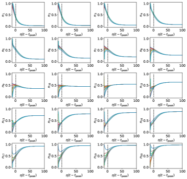
Figure S9: Time evolution of the mean occupation in real space $\langle n_{i}\rangle$ from kinetic theory for a half-filling chain under a linear potential described by Hamiltonian (1). The vertical dashed lines marks the time of reaching peak entropy. The initial states are different Fock states with high energies. The parameters are $M=20$, $r=4J$, $\eta=0.1J$.

Disordered Potential

Fig. S10(a) shows the rate matrix for a Fermi-Hubbard chain under a disordered potential with random on-site energies uniformly drawn from the interval $[-W,W]$ coupled to a thermal bath. It has a non-local structure, which is different from that of the Stark model in the main text [see Fig. 2(b)]. Such a rate matrix can not give rise to a close-to-maximum peak entropy, as shown in Fig. S10(b).

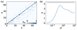
Figure S10: (a) Rate matrix for a Fermi-Hubbard chain under a disordered potential with disorder strength $W=20J$ coupled to a thermal bath. (b)  Time evolution of entropy. The initial state is the highest excited state. The results are for one disorder realization. The parameters are $M=8$, $V=J$, $\eta=0.1J$, $T$ is chosen to make $S_{T}=S_{\infty}/2$.

Optimized potential model

Figure S11 shows time evolution of entropy $S=-\sum_{k}p_{k}\log(p_{k})$ for a half-filling chain (described by Hamiltonian (1) with the on-site potential $W_{i}$ shown in the inset) coupled to a thermal bath. The dynamics of $p_{k}$ is governed by rate equation. The distribution $p_{k}$ at the three different times marked by vertical lines in (a) is shown by solid lines in (b). It is found to be close to a thermal distribution, analogous to the Stark model [see Fig. 1(f) in the main text].

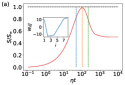
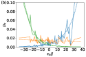
Figure S11: (a) Time evolution of entropy $S=-\sum_{k}p_{k}\log(p_{k})$ for a half-filling chain (described by Hamiltonian (1) with the on-site potential $W_{i}$ shown in the inset) coupled to a thermal bath. The dynamics of $p_{k}$ is governed by rate equation (S7). (b) Distribution of $p_{k}$ at three moments marked in (a) are shown in solid lines, which is close to the distribution of the corresponding thermal states with the same average energy shown in dashed lines. The parameters are $M=8$, $V=J$, $\eta=0.1J$, $T$ is chosen to make $S_{T}=S_{\infty}/2$.

Simplified models

Figure S12 shows the normalized peak entropy $S_{\rm peak}$ and thermal entropy $S_{T}$ for the simplified model where $p_{k}$ is governed by $\dot{p}_{k}=\eta(\bar{R}\nabla^{2}p_{k}+\delta R\nabla p_{k})$ starting from the highest excited state. In (a)-(c), the dependence of $S_{\rm peak}$ and $S_{T}$ on $\alpha=\delta R/\bar{R}$ for three different system dimensionality ${\cal D}$ is shown. In (d)-(f), the dependence of $S_{\rm peak}$ and $S_{T}$ on ${\cal D}$ for three different ${\alpha}$ is shown. The results indicate the existence of a non-trivial parameter regime with both $S_{\text{peak}}\approx S_{\infty}$ and $S_{T}$ well below $S_{\infty}$.

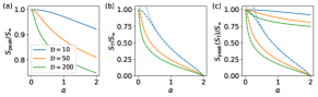
Figure S12: The peak entropy ($S_{\rm peak}$) and the thermal entropy ($S_{\rm T}$) (normalized by the maximum entropy $S_{\infty}=\log({\cal D})$) as a function of (a)-(c) $\alpha\equiv\delta R/\bar{R}$ and (d)-(f) ${\cal D}$. The entropy is calculated as $S=-\sum_{k}p_{k}\log(p_{k})$, with $p_{k}$ governed by rate equation (S7). The initial state is $p_{k}=\delta_{k,{\cal D}-1}$ for $0\leq k\leq{\cal D}-1$. The dotted lines are from the expression $S_{T}=\frac{x}{x-1}\log(x)-\log(1-x)$ with $x=(2-\alpha)/(2+\alpha)$.

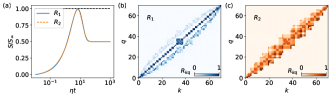
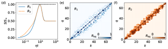
Figure S13: (a) Time evolution of the entropy $S=-\sum_{k}p_{k}\log(p_{k})$ with $p_{k}$ governed by rate equation (S7) under two different rate matrices shown in (b) and (c). The initial state is the highest excited state. The parameters are $M=8$, $V=0$, $r=4J$, $\eta=0.1J$, $\epsilon=0.15$. (d)-(f) show the corresponding results for interacting system with $V=J$. The fitting parameter is $\epsilon=0.22$ in this case.

In Fig. S13(a) we show the time evolution of entropy $S=-\sum_{k}p_{k}\log(p_{k})$ with $p_{k}$ governed by rate equation under two different rate matrices shown in (b) and (c). The former ($R_{1}$) is the real rate matrix of the noninteracting Stark model. It depends on both the bath correlation function and the overlap of wave functions, i.e., $R_{kq}=\pi v_{kq}g(\varepsilon_{k}-\varepsilon_{q})$ with $v_{kq}=\sum_{i}{|\langle k|n_{i}|q\rangle|^{2}}$, which endows it a complex texture. The rate matrix $R_{2}$ used in (c) is obtained from $R_{1}$ by replacing $v_{kq}$ by the binary values $\epsilon$ or $0$, depending on whether $|v_{kq}|>0.1$ or $<0.1$, respectively. As shown in Fig. S13(a), the entropies for these two rate matrices are found to be almost the same. In (d)-(f), we show the corresponding results for interacting system with $V=J$.