Meta Adaptation using Importance Weighted Demonstrations

Abstract

Imitation learning has gained immense popularity because of its high sample-efficiency. However, in real-world scenarios, where the trajectory distribution of most of the tasks dynamically shifts, model fitting on continuously aggregated data alone would be futile. In some cases, the distribution shifts, so much, that it is difficult for an agent to infer the new task. We propose a novel algorithm to generalize on any related task by leveraging prior knowledge on a set of specific tasks, which involves assigning importance weights to each past demonstration. We show experiments where the robot is trained from a diversity of environmental tasks and is also able to adapt to an unseen environment, using few-shot learning. We also developed a prototype robot system to test our approach on the task of visual navigation, and experimental results obtained were able to confirm these suppositions.

I Introduction

In recent years, we have seen many agents perform numerous tasks using Imitation learning, in countless applications, especially robotics. There has been a significant progress made for algorithms which learn amidst noisy environments [9], sparse training signals [26], and imperfect demonstrations [10]. However, there has not been much focus on allowing these agents to gather data and generalize to a wide variety of environments.

Especially for the task of navigation, this is quite crucial because, autonomous navigation systems like self-driving cars, delivery robots should be able to function in almost any situations [\cite[cite]{[\@@bibref{}{DBLP:conf/icra/LekkalaI21, 21, 22, 23, lekkala2016simultaneous}{}{}]}]. Since the data distribution continuously changes, it is challenging to learn a task from a fixed set of data, nor is it practical to obtain a comprehensive dataset [4]. In nearly every real-world applications, the data distribution is long-tailed, meaning that the agent would always encounter new patterns, which has a small number of examples. There would always be instances where the agent has never encountered in the past. Taking a step forward, we would then want these systems to perform well in any given situation by applying prior patterns. Although we are concerned about navigation, researchers from other backgrounds can also find related reasons to concur with us.

Many of the existing solutions restrict their data domain, by training and testing on datasets collected on same environments [\cite[cite]{[\@@bibref{}{wen2022can, 36, 11, lekkala2020attentive}{}{}]}]. Other works like [2], apply their algorithm to self-driving cars, have a much broader data domain. However, since these models were not trained in different settings, for example, cluttered, pedestrian-rich environment, they would not generalize to other settings. Some of the recent works, which try to generalize to new contexts are quite promising but also have some loopholes. With all these practical considerations, it is imperative that we design a method which enables the algorithm to function in diverse scenarios.

Meta-Learning deals with applying prior knowledge from various skills to learn a new skill in a few shot setting. These algorithms facilitate the model to utilize previous experience by constructing reusable structured patterns which could then be adapted in new contexts. We propose a method which meta-learns a set of tasks and generalizes to new tasks using a few samples. This paper deals with the first step in making an agent adapt to dynamically changing environments.

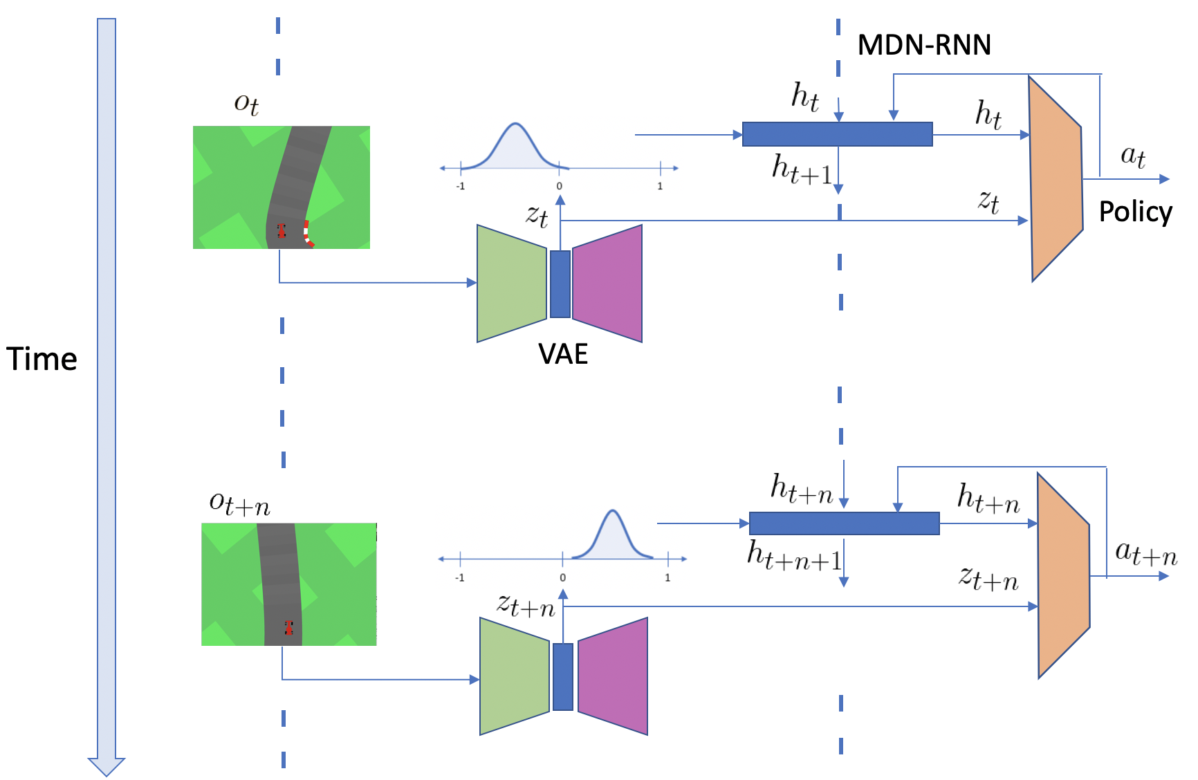
Figure 1: Pictorial representation of world model in action

II Background and Related Work

Direct Policy Search is a class of policy estimation algorithms which find the parameters of the model by optimizing a predefined cost function, which can be with respect to a reward function or expert demonstrations. For a single task, methods on the aspect of Learning a policy from expert demonstrations have been seen to be predominant in the past [16, 3, 15, 18]. For more complicated tasks involving non-stationary data distribution [6], methods involve gathering the expert data [29], and training a predictive model. Recently, a lot of methods as outlined by [1] were proposed in the aspect of model fitting on the expert data for an agent. These methods mainly deal with mitigating, covariate shift, where the input distribution or the training data changes, but the conditional distribution of labels given the data remains fixed [27]. On the other hand, several other works address this problem from an other angle, [1, 19, 33], especially DAGGER [29] using active learning [14]. Out of all, we choose DAGGER to train our model as it simple and works well in practical cases. A number of works have been applied to the task of navigation, like [4, 25]

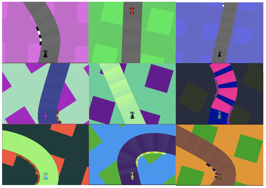
Figure 2: Pictures of different car-racing simulators used. Environments in the first row are used for training tasks, and all the other environments were used as test tasks.

Some of the significant improvements in Imitation learning involve making algorithms robust to long-horizon tasks or changing data distribution [24, 20]. Other works, which follow a similar trend, include partitioning the domain into individual tasks and making the model train using multiple tasks [35]. An enhancement of multi-task imitation learning, i.e., hierarchical imitation learning, involves high-level planners to estimate sub-goals for the low-level policies [37]. Although these methods perform better than naive Imitation learning, most of them do not generalize to new related tasks.

Many recent works on few-shot imitation learning [12, 5, 8] involve novel meta-learning schemes. The basic principle underlying all these works involve adapting and inferring model to unseen tasks. Some of the novel approaches used by these methods are hybrid loss functions [5], evolving policy gradients [17], and estimating meta parameters [7]. The core idea of most of the works mentioned above involve parameter adaption for unseen tasks. Some of the few recent works which apply meta-learning to Visual Navigation are [30, 34]. Compared to others, the meta objective of our adaptive approach relies on the alignment of the evaluated gradients on training data to the test data. Previously, variants of these approaches were used in supervised learning, for minimizing distribution shift between training and test datasets [28]. Our main contributions are outlined as follows:

1$\cdot$ We propose a novel Importance Weighting method to amplify the gradients evaluated on the training demonstrations for better performance on the test task.

2$\cdot$ Our method is robust on dynamically changing distributions, and can also be extended to Meta Imitation learning, where an agent needs to quickly learn an unseen related task from prior experiences.

3$\cdot$ To the best of our knowledge, we are the first to apply iteratively trained world models, along with our proposed improvements, to the task of Imitation learning

This paper has been organized as follows. In Section III, World models and our improvements are illustrated. Then, In Section IV, out main contribution is outlined. After that, different experiments performed and the related observations are explained in V and VI respectively, followed by conclusion.

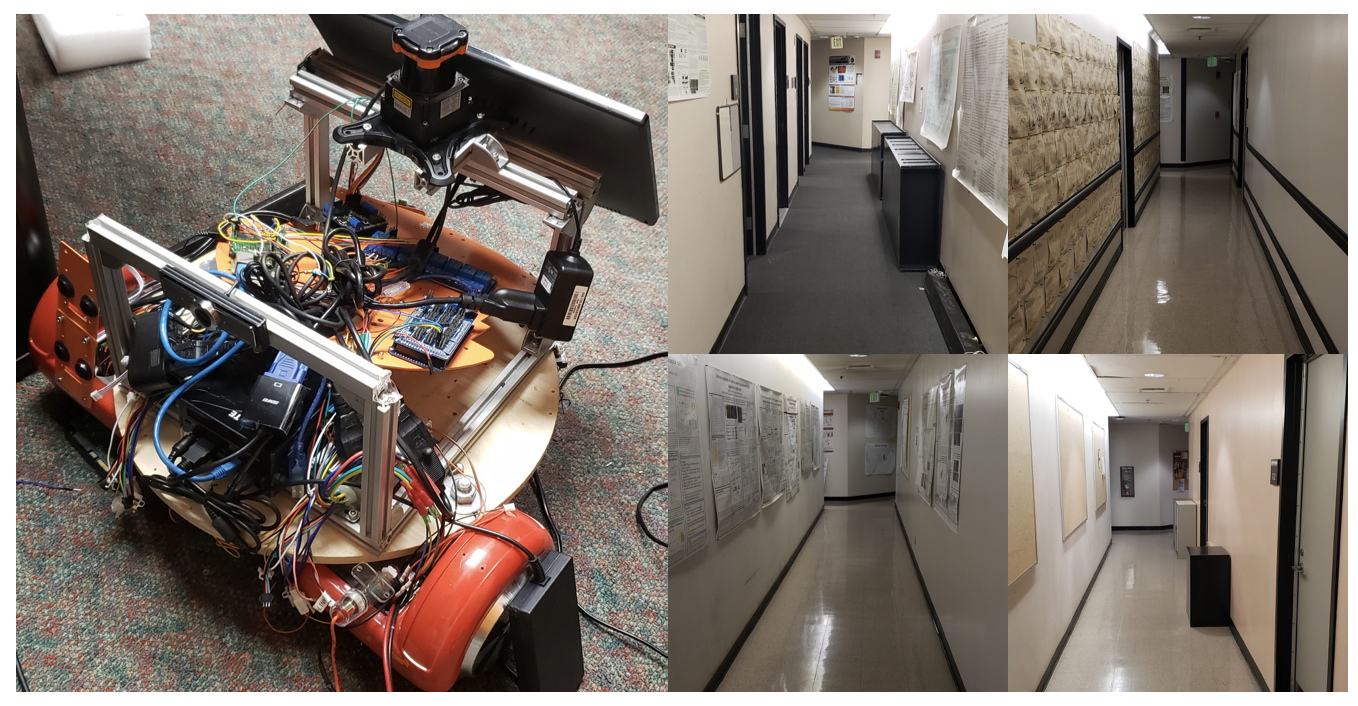
Figure 3: Picture of the physical robot used to test our method. On the right side, the real-world environments used for evaluating our model are pictured.

III Imitation learning using World models

Instead of learning the parameters by training the model end to end like [4], an Itervative training procedure using World models [13] is adapted. We hypothesize that modularizing a model and training each component individually works well for many tasks. We corroborate this hypothesis with previous works in Neuroscience such as [31, 32]. This methodology also performs well for meta-learning scenarios, where the end policy alone can be retrained for new tasks by leaving prior modules fixed , as it will be clear in the later sections.

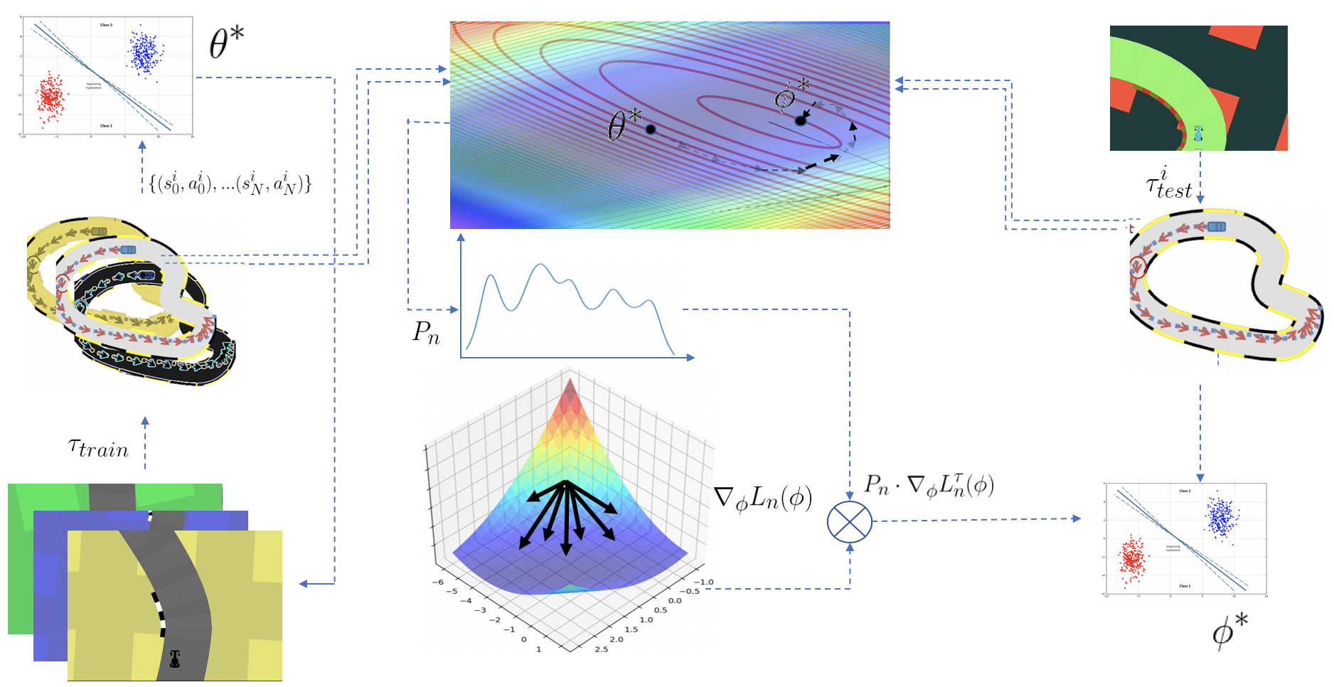
Figure 4: Working of our method. On the left side, the training procedure is mentioned. The agent is trained on a variety of environments. During test time, our method enables the agent has to adapt to a new environment.

III-A Prelimnaries

A World model (Figure 1) consists of a Variational Autoencoder (VAE), Mixture Density Recurrent Neural Network (MDN-RNN) and a Neural Network (Policy). Each of these modules are named as Vision (V), Memory (M) and Controller (C) modules. Note that in the remainder of the paper, we will be using policy and controller interchangeably.

When a world model is evaluated on a specific task, say $\mathcal{T}^{i}$, we obtain a set of observation-action pairs $\{\langle O^{i}_{j}$, $a^{i}_{j}\rangle\}_{j=0}^{j=T}$. During training, A VAE, encodes an observation $O_{i}^{j}$ to a latent variable $z_{j}$ which is sampled from a Normal distribution $z\in\mathcal{N}(\mu,\Sigma)$. In tasks like navigation where the current state is conditional on the previous state and action, we have a transition model (MDN-RNN) which models $p(z_{j+1}|z_{j},a_{j})$. Specifically, MDN-RNN emits $h_{t}$ at every time-step, which contains the transition probabilities. A state is a vector formed by concatenating $h_{j}$ and $z_{j}$. In the case of Model-free approaches, $s_{j}$ would just be $z_{j}$. Given this state, a policy is a single layer neural network $f(s_{j},\theta)$

III-B Improvements on existing World Models

To train the V and M modules, Instead of spawning trajectories with a random policy [13], we use a trained policy to collect data. We performed some experiments, where we found that reproducing the original World model experiments on an V and M trained on data from an expert policy, resulted in better performance. We also found that World models generalize very well, even with small amounts of data trajectories, (of the order 10-20), which makes them suitable for applying in real-world settings.

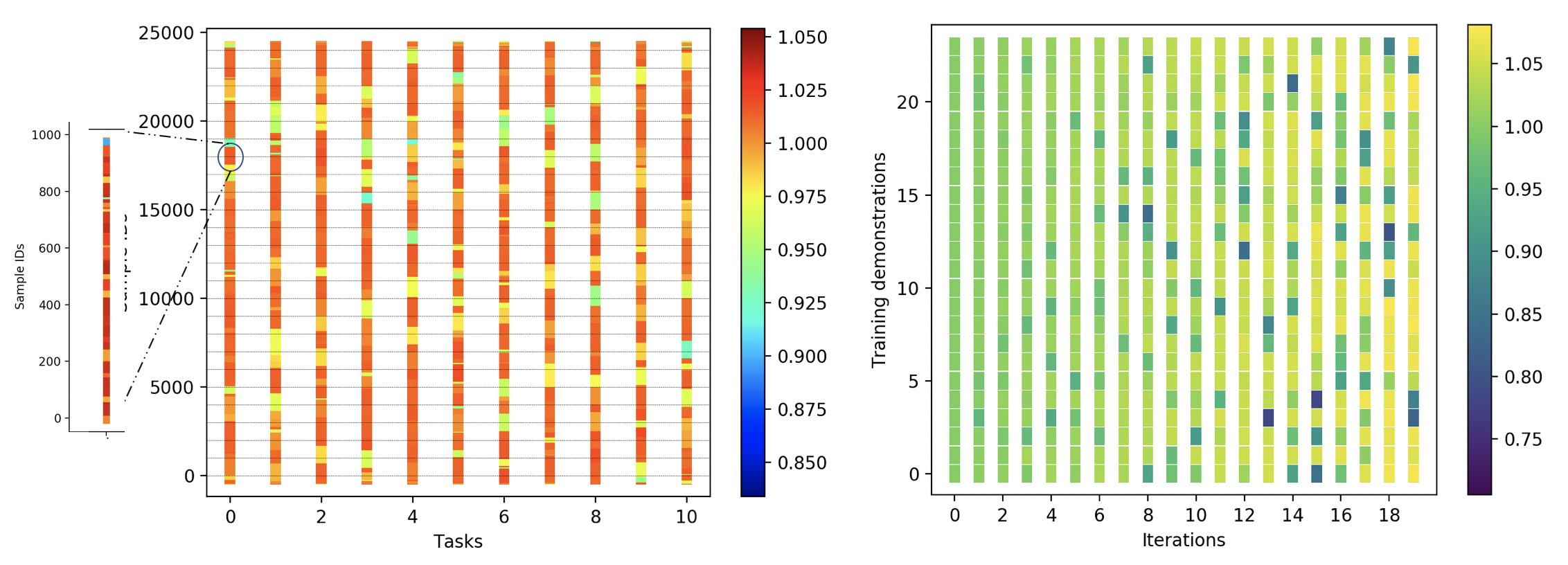
Figure 5: (a) Colormap of $p$ values after $\phi^{i}$ converges on 10 different tasks. The dashed line represents the trajectories. An instance of the $p$ values of a trajectory is enlarged for better visualization. (b) Change of $p$ values over time. We evaluated our algorithm on a specific task to show how the $p$ values change over every iteration.

III-C Active learning for policy estimation

In this work, we train world models using Imitation learning by employing DAGGER as proposed by [29]. DAGGER is an active learning-based method which involves giving control to the agent to gather training data. The policy is then trained by aggregating data over each trial on the environment. We used the original world model [13] as an expert world model and our improved world model as the agent’s model. The policy parameters of the original world model were trained using Reinforcement learning and performed particularly well, even amidst any disturbances or noise, in the environment. This specific trait made it the right choice for an expert in this case, as in many situations, the agent would go to a vulnerable state, and the expert should recover from such erratic behavior. In the case of the real-world robot, we do not have such a robust expert yet, and so we used a human demonstrator.

IV Proposed method

The main contribution is outlined. The code related to our method can be found at https://github.com/kiran4399/weighted_learning.

IV-A Problem formulation

We consider a Meta-Supervised learning setting, where the agent has access to the distribution of training tasks $p(\mathcal{T}_{train})$ at train-time. To train the policy, we require a set of expert demonstrations $\{\langle s^{i}_{j},\hat{a}^{i}_{j}\rangle\}_{j=0}^{j=T}$, where the $T$ is the length of an episode, on the set of train tasks $\mathcal{T}^{i}_{train}$ to estimate $\theta^{*}$ which minimizes the log-likelihood, on the expert data. The goal of the agent is to generalize to new test task $\mathcal{T}^{i}_{test}$ using a few samples. The train and test datasets consist of the data aggregated on the training tasks and the test specific task, respectively. $\theta^{*}$ is $\theta$ after convergence on the training dataset and, is used to initialize $\phi^{i}$, which are the policy parameters required to train on the test data obtained on a specific task.

IV-B Assigning Importance weights

In general, Imitation learning is based on optimizing a model maximize the log-likelihood which is represented in the following equation, where $f$ is the model and $N$, $s_{n}$, $\hat{a}_{n}$ are the number of samples, states and actions respectively.

$$\mathcal{L}(\theta)=\frac{1}{N}\sum_{n=0}^{n=N}\hat{a}_{n}\log(f(s_{n}))$$ (1)

$$\theta^{*}=\operatorname*{arg\,max}_{\theta}\frac{1}{N}\sum_{n=0}^{n=N}\mathcal{L}(\theta)$$ (2)

However, as mentioned before, maximizing the average likelihood may not yield the desired outcome in a lot of applications because of some training samples being irrelevant, noisy or unevenly distributed. We can correct the covariate shift by estimating a non-trivial distribution of scalar weights, estimated from a small data batch drawn from an optimal distribution [13]. Compared to Eqn 2, the optimal parameters and the gradient of the Loss function with respect to parameters $\phi$ becomes:

$$\phi^{*}=\operatorname*{arg\,max}_{\phi}\sum_{n=0}^{n=N}P_{n}\mathcal{L}(\phi)$$ (3)

$$\begin{split}\nabla_{\phi}\mathcal{L}(\phi)&=\sum_{n=0}^{n=N}P_{n}\cdot\nabla_{\phi}\mathcal{L}_{n}(\phi)\end{split}$$ (4)

In the above equation, $P$ is a vector of the size of training samples and adapts based on the training and test data. For meta-imitation learning, we can use same method to learn the task distribution shift and make the training adapt to different perturbed scenarios. In other words, during test-time, we can evaluate gradients $\nabla_{\phi}L(\phi)$ on task-specific demonstrations $\mathcal{D}_{test}$ and impose them on the per-sample gradients $\nabla_{\phi}\mathcal{L}_{n}(\phi)$ estimated on the training data $\mathcal{D}_{train}$, where $\phi^{i}$ are the policy parameters.

Initially, we train the policy parameters $\theta$ on a sampled set of train tasks $\mathcal{T}^{i}_{train}$ to collect training data Note that, $\theta$ and $\phi$ are the parameters of the policy at train and test time respectively. We could have used $\theta^{i}$, instead of $\phi^{i}$, but we use that notation for parameters which are obtained by training the policy only on the test task $\mathcal{T}_{test}^{i}$.

During test time, when we asses the generalization ability of a policy on an unseen test task, we train the policy likewise to the training approach, but only using the test data. We, however, use the test data to learn the $P$ distribution and calculate the dot product, represented by $\mathbin{\vbox{\hbox{\scalebox{0.5}{$\bullet$}}}}$ with the per sample gradients, which we use to update $\phi$. For simplicity sake superscript $i$ is omitted. The distribution $P$, which is a vector of size $N$, can be updated by optimizing the cost function $J(P,\phi)$ of the L2 distance between $\nabla_{\phi}L(\phi)$ and $\nabla_{\phi}\mathcal{L}(\phi)$ for each batch of test and train data. Note that if the dimensionality of the average gradients $\nabla_{\phi}L(\phi)$ is $\mathcal{R}^{a\times b}$, the dimensions of $\nabla_{\phi}\mathcal{L}(\phi)$ would be $\mathcal{R}^{N\times a\times b}$ Also, we apply softmax over distribution parameters $p_{n}$ such that $P_{n}$ always sum to 1. The gradient of the cost function with respect to $P$ is as follows.

$$\frac{\partial}{\partial P}J(P,\phi)=\frac{\partial}{\partial P}\left(P\mathbin{\vbox{\hbox{\scalebox{0.5}{$\bullet$}}}}\nabla_{\phi}\mathcal{L}_{n}(\phi)-\nabla_{\phi}\hat{\mathcal{L}}(\phi)\right)^{2}$$ (5)

$$\nabla_{P}J(P,\phi)=\left[\nabla_{\phi}L_{n}(\phi)^{T}\mathbin{\vbox{\hbox{\scalebox{0.5}{$\bullet$}}}}\left[P_{n}\mathbin{\vbox{\hbox{\scalebox{0.5}{$\bullet$}}}}\nabla_{\phi}\mathcal{L}_{n}(\phi)-\nabla_{\phi^{{}^{\prime}}}L(\phi)\right]\right]^{T}$$ (6)

During every iteration, apart from updating $\phi$ using our method, we also update the distribution parameters $p_{n}$, for $K$ iterations. Using the analytical gradient computed in Eqn 6, we can compute the gradient with respect to $p$ using chain rule as follows.

$$\frac{\partial J}{\partial p}=\frac{\partial J}{\partial P}\mathbin{\vbox{\hbox{\scalebox{0.5}{$\bullet$}}}}\frac{\partial P}{\partial p}$$ (7)

$$\nabla_{p}J(p,\phi)=\nabla_{P}J(P,\phi)\mathbin{\vbox{\hbox{\scalebox{0.5}{$\bullet$}}}}\nabla_{p}\sigma(p)$$ (8)

In the above equation $\nabla_{p}\sigma(p)$ is the gradient of the softmax function, which is a $N\times N$ matrix. The policy parameters $\phi^{i}$ are thus, iteratively learned by utilizing the training data, but deriving the $P$ distribution from the test data. A synopsis of the entire algorithm is illustrated on the next page.

Algorithm 1 Estimate $\theta^{*}$ and $\phi^{i^{*}}$

0:  $p(\mathcal{T}_{train})$ and $p(\mathcal{T}_{test})$ as task distributions

0:  $\alpha$, $\beta$ and $\gamma$ as step-size parameters

0:  Expert policy $\hat{\theta}$

1:  Sample tasks $\mathcal{T}^{i}$ from task distribution $p(\mathcal{T}_{train})$

2:  Evaluate $\hat{\theta}$ on $\mathcal{T}^{1},\mathcal{T}^{2},..,\mathcal{T}^{M}$ to collect {$O_{j}^{i}$, $\hat{a}_{j}^{i}$}

3:  Train VAE and MDN-RNN (Refer Section III)

4:  Randomly initialize $\theta$

5:  for each sampled task $\mathcal{T}^{i}$ from $p(\mathcal{T}_{train})$ do

6:    Evaluate $\theta_{\tau}$ on $\mathcal{T}^{j}_{train}$ to generate $\mathcal{D}^{i}_{train}$

7:    $\mathcal{D}_{train}\leftarrow\mathcal{D}_{train}\cup\mathcal{D}^{i}_{train}$

8:    for $t\in\{0,1,..\tau$ } do

9:       Evaluate gradients on $\mathcal{D}_{train}$ at $\theta_{t}$

10:       $\theta_{t+1}\leftarrow\theta_{t}-\alpha\nabla_{\theta}L(\theta_{t})$

11:    end for

12:  end for

13:  Sample tasks $\mathcal{T}^{i}$ from $p(\mathcal{T}_{test})$

14:  for each task $\mathcal{T}^{i}$ do

15:    Initialize $\phi^{i}$ = $\theta^{*}$

16:    for $t$ in {0, 1, .. $\hat{\tau}$ } do

17:       Evaluate $\phi^{i}_{t}$ on $\tau^{i}_{test}$ to generate $\mathcal{D}_{test}$

18:       for $k\in{0,1,...K}$ do

19:          Evaluate $\nabla_{\phi}L(\phi_{t})$ on $D^{i}_{test}$

20:          Calculate $\nabla_{P}J(P,\phi)$ From Eq 8.

21:          $\nabla_{p}J(p,\phi^{i})=\nabla_{P}J(P,\phi^{i})\mathbin{\vbox{\hbox{\scalebox{0.5}{$\bullet$}}}}\nabla\sigma$

22:          $p_{k+1}\leftarrow p_{k}-\gamma\nabla_{p}J(p,\phi)$

23:       end for

24:       $\phi^{i}_{t}\leftarrow\phi^{i}_{t}-\beta\nabla_{\phi}\hat{L}(\phi_{t})$

25:    end for

26:  end for

V Experimental setup

V-A Experiments on simulator

We used a Car Racing simulator from OpenAI gym to test our method. We adapted a world-model from [13] by retraining the architectures for the VAE and MDN-RNN, using different hyperparameters. The controller/policy was changed to a single layer classifier to categorize a state to one of the five discretized actions. We chose to use a single layer policy, as simple architectures tend to generalize better. We created multiple car racing environments and considered them as tasks. We collect 24 expert trajectories, 4 for each task, and use them as the training data.

For policy training, we used Stochastic Gradient Descent (SGD) with step-size parameters $\alpha$, $\beta$ and $\gamma$ as $0.01$, $0.01$ and $0.05$ respectively. We limited $K$ updates to 10, as we found this to be sufficient for the experiments. We set $\tau$ to 3000 and 4000 iterations for training and testing respectively. We encourage the reader to refer to the algorithm in the previous page for the notations.

V-B Physical setup

We also evaluated our method using a physical system, in our case a Non-Holonomic, differential-drive based robot for the task of visual navigation. For real-world experiments, we defined a task as the environment on a specific level in the building. Each level was visually very distinct from the other, and we interpreted an environmental seed as a unique source and destination location on a particular level of the building. Images obtained from a camera, mounted on the robot, were timestamped and synced with the action commands before being sent for training. We used ROS and Tensorflow for implementing our experiments.

We used a world model with similar modifications applied to the simulator experiments. We collected 30 human-controlled trajectories, 10 for each task, and trained the V and M modules. The robot was then tested on the remaining one environment, which it had not seen before.

VI Observations and Results

Compared to the state of the art benchmark [13] on the car-racing simulator, our method deals not so much with the maximum score in a given episode but how quickly it can learn an optimal behavior and adapt to a related unseen environment. Following are some of the observations, which we had found.

VI-A Generalization to unseen Tasks

Apart from the training data, We also generated some environments as test tasks for the model. Though none of the components of the world model were trained on those tasks, our method made the world model generalized to them. We also added uniform Gaussian noise on all the observations of the test tasks for robustness. To compare our method, we used 2 baselines: DAGGER baseline ($\theta^{*}$) which was trained by aggregating the data from all the prior tasks and the test task and Fine-tuning baseline ($\theta^{i^{*}}$) which was trained the policy only on the test task. Figure 7 shows that our method outperformed these baselines. As a primary measure, we used the number of times the expert had to intervene to allow the agent to get off a vulnerable state, which we call override. We also portrayed the mean accuracies on different tasks for each baseline, as we wanted the reader to notice the relationship between accuracy and overrides as an appropriate measure for comparing baselines. We argue that both of them are required in active imitation learning, as a model might have a high average accuracy, but might not perform well on some important states. For quantitative comparison on different baselines, refer Table I

VI-B Converging to local optima for train tasks

Usually, in Meta-learning, the goal for the classifier is the generalize to unseen tasks from the prior information obtained from the train tasks. However, in some scenarios, like that of navigation, we want the agent to perform well on the training tasks as well. After $\theta$ convergence, we evaluate the policy on each training tasks, sampled with random seeds and added Gaussian noise. Surprisingly, the agent performed sub-optimally on every task. Since the world model was trained on the training tasks, Naively aggregated data should’ve performed well. However, in situations, where there are a sufficiently large number of tasks, the model would collapse to a local optimum. However, when we ran used our method for on a specific train task as a test task for 1 iteration. it resulted in better performance.

VI-C Robustness amongst noise in demonstrations

Our algorithm works well, even in cases where there is noise in the collected demonstrations. During training, in each iteration of policy evaluation, we randomly select 50 % of the collected demonstrations and corrupt the action labels. Even in such scenarios, our algorithm remains robust by giving those corrupted samples less importance, i.e., less $p$ values and performing well on the test task. Figure 6 states the results.

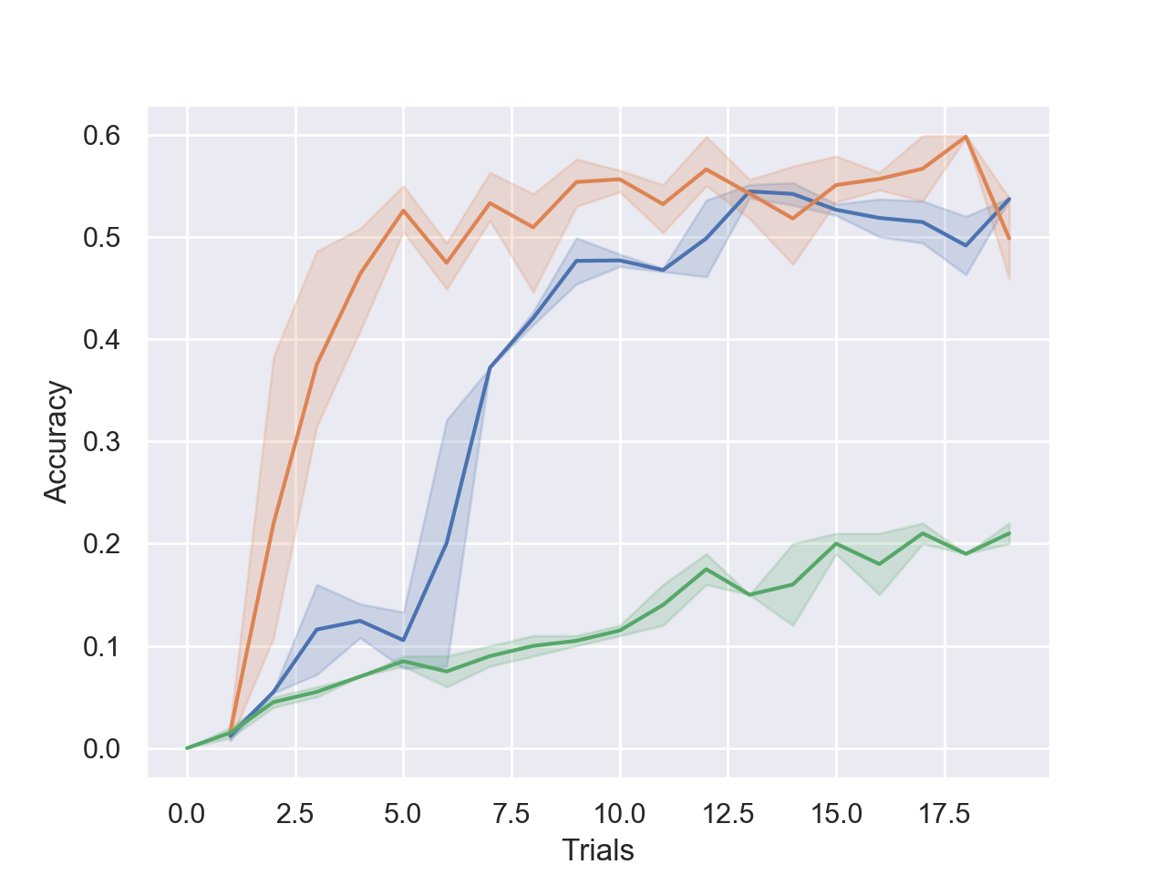
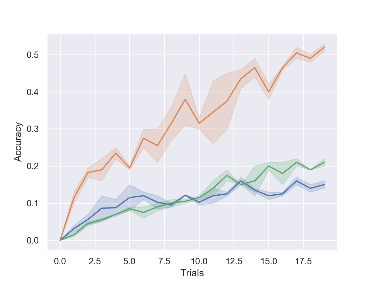
Figure 6: Plots corresponding to (a) Comparison of training loss with time for $\theta^{*}$ (orange) and $\theta^{i^{*}}$ (blue) during training (b) Comparision of training loss on training data and test data of $\phi^{i^{*}}$ on a randomly sampled Unseen task. (c) Comparison of the Accuracy of $\theta^{*}$ (green), $\theta^{i^{*}}$ (blue) and $\phi^{*}$ (orange) on a Clean dataset (lower left) Noisy dataset (lower right), for a set of 4 unseen tasks.

VI-D Visualization of the P values

Although we performed many experiments confirming the robustness of our algorithm, it is important to understand the $p$ values in each case, to know which of the samples are getting more importance. Note that, each aggregate training sample, which are in total 24k, has a $p$ value associated with it. In Figure 5, we provide a color map of the $p$ values, after $\phi^{i}$ converges. Although it is unclear, how the samples having high $p$ are related to the test task, we can comprehend that the model is able to learn the new task from the prior tasks. In the same figure, we also show how the $p$ values change with each trial, which indicates that, the sample importance, changes with getting more information from the new test task.

VI-E Experiments in real-world

We ran our robot on the corridors in the Hedco Neuroscience building at the University of Southern California. Though the geographical and structural maps of each floor were similar, the visual features were very different, which makes it perfect for applying our method. Pictures taken in different floors are depicted in Figure 3. Results obtained by test the robot in different environments are shown in Table I

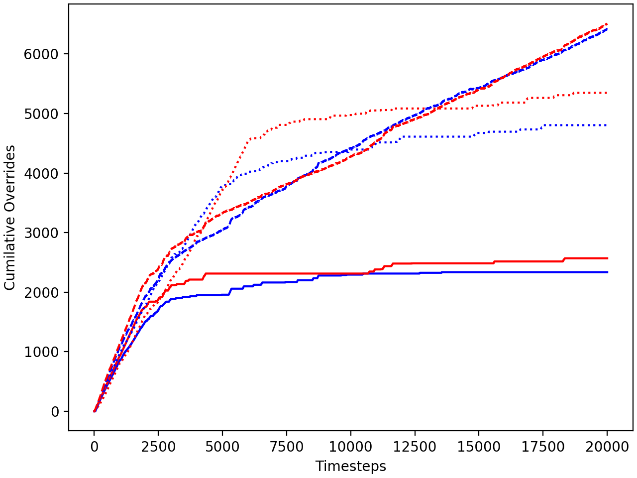
Figure 7: Comparision of 2 different tasks (marked with red and blue) on which the model was evaluated. The plain, dotted and dashed curve represents the performance of $\theta^{*}$, $\theta^{i^{*}}$ and $\phi^{i^{*}}$ baselines respectively. We can see that our method outperforms other baselines. The $y$ axis represents the cumulative number of overrides over the trials, and the $x$ axis represents timesteps of all the trials combined.

TABLE I: Quantitative of the baselines. The results given in the following 2 tables correspond to the Car Racing simulator and the real world environments respectively. The values mentioned in each cell correspond to the accuracies of the policy after training on the number of trials.

Method	1 Trial	2 Trials	5 Trails
DAGGER	$5.1\pm 0.8\%$	$6.2\pm 1.3\%$	$8.5\pm 1.1\%$
Fine-tune	$9.2\pm 0.9\%$	$12.6\pm 1.5\%$	$17.9\pm 2.8\%$
Ours	$\mathbf{21.5\pm 5.1\%}$	$\mathbf{39.7\pm 7.2\%}$	$\mathbf{53.2\pm 3.3\%}$

Method	2 Trial	5 Trials	10 Trails
DAGGER	$3.5\%$	$7.1\%$	$7.9\%$
Fine-tune	$8.1\%$	$9.3\%$	$13.1\%$
Ours	$\mathbf{18.2\%}$	$\mathbf{23.5\%}$	$\mathbf{31.6\%}$

VII Conclusion

In this paper, we presented a Meta-Imitation learning algorithm which involves learning new skills from prior knowledge. We defined a task or skill as an environment having a specific data distribution attributed by time or situation. applications, which involves substantial covariate shifts, by considering it as a meta-learning problem. We have also shown how the proposed algorithm can be used to improve the policy performance on a single task, which was trained on a set of tasks Some of our experiments performed using a real robot, shows how our algorithm can aid real-world scenarios as well. The results shown on the task of navigation support our assertions.

References

- [1] Alexandre Attia and Sharone Dayan “Global overview of Imitation Learning” In CoRR abs/1801.06503, 2018 arXiv: http://arxiv.org/abs/1801.06503
- [2] Mariusz Bojarski et al. “End to End Learning for Self-Driving Cars” In CoRR abs/1604.07316, 2016 arXiv: http://arxiv.org/abs/1604.07316
- [3] Sonia Chernova and Manuela M. Veloso “Confidence-based policy learning from demonstration using Gaussian mixture models” In 6th International Joint Conference on Autonomous Agents and Multiagent Systems (AAMAS 2007), Honolulu, Hawaii, USA, May 14-18, 2007, 2007, pp. 233 DOI: 10.1145/1329125.1329407
- [4] Felipe Codevilla et al. “End-to-End Driving Via Conditional Imitation Learning” In 2018 IEEE International Conference on Robotics and Automation, ICRA 2018, Brisbane, Australia, May 21-25, 2018, 2018, pp. 1–9 DOI: 10.1109/ICRA.2018.8460487
- [5] Yan Duan et al. “One-Shot Imitation Learning” In Advances in Neural Information Processing Systems 30: Annual Conference on Neural Information Processing Systems 2017, 4-9 December 2017, Long Beach, CA, USA, 2017, pp. 1087–1098 URL: http://papers.nips.cc/paper/6709-one-shot-imitation-learning
- [6] Peter Englert, Alexandros Paraschos, Jan Peters and Marc Peter Deisenroth “Model-based imitation learning by probabilistic trajectory matching” In 2013 IEEE International Conference on Robotics and Automation, Karlsruhe, Germany, May 6-10, 2013, 2013, pp. 1922–1927 DOI: 10.1109/ICRA.2013.6630832
- [7] Chelsea Finn, Pieter Abbeel and Sergey Levine “Model-Agnostic Meta-Learning for Fast Adaptation of Deep Networks” In Proceedings of the 34th International Conference on Machine Learning, ICML 2017, Sydney, NSW, Australia, 6-11 August 2017, 2017, pp. 1126–1135 URL: http://proceedings.mlr.press/v70/finn17a.html
- [8] Chelsea Finn et al. “One-Shot Visual Imitation Learning via Meta-Learning” In 1st Annual Conference on Robot Learning, CoRL 2017, Mountain View, California, USA, November 13-15, 2017, Proceedings, 2017, pp. 357–368 URL: http://proceedings.mlr.press/v78/finn17a.html
- [9] Roy Fox, Ari Pakman and Naftali Tishby “Taming the Noise in Reinforcement Learning via Soft Updates” In Proceedings of the Thirty-Second Conference on Uncertainty in Artificial Intelligence, UAI 2016, June 25-29, 2016, New York City, NY, USA, 2016 URL: http://auai.org/uai2016/proceedings/papers/219.pdf
- [10] Yang Gao et al. “Reinforcement Learning from Imperfect Demonstrations” In 6th International Conference on Learning Representations, ICLR 2018, Vancouver, BC, Canada, April 30 - May 3, 2018, Workshop Track Proceedings, 2018 URL: https://openreview.net/forum?id=HytbCQG8z
- [11] Yunhao Ge et al. “Lightweight Learner for Shared Knowledge Lifelong Learning” In CoRR abs/2305.15591, 2023 DOI: 10.48550/arXiv.2305.15591
- [12] Abhishek Gupta et al. “Learning Invariant Feature Spaces to Transfer Skills with Reinforcement Learning” In 5th International Conference on Learning Representations, ICLR 2017, Toulon, France, April 24-26, 2017, Conference Track Proceedings, 2017 URL: https://openreview.net/forum?id=Hyq4yhile
- [13] David Ha and Jürgen Schmidhuber “Recurrent World Models Facilitate Policy Evolution” In Advances in Neural Information Processing Systems 31: Annual Conference on Neural Information Processing Systems 2018, NeurIPS 2018, 3-8 December 2018, Montréal, Canada., 2018, pp. 2455–2467 URL: http://papers.nips.cc/paper/7512-recurrent-world-models-facilitate-policy-evolution
- [14] He He, Hal Daumé III and Jason Eisner “Imitation Learning by Coaching” In Advances in Neural Information Processing Systems 25: 26th Annual Conference on Neural Information Processing Systems 2012. Proceedings of a meeting held December 3-6, 2012, Lake Tahoe, Nevada, United States., 2012, pp. 3158–3166 URL: http://papers.nips.cc/paper/4545-imitation-learning-by-coaching
- [15] Todd Hester et al. “Deep Q-learning From Demonstrations” In Proceedings of the Thirty-Second AAAI Conference on Artificial Intelligence, (AAAI-18), the 30th innovative Applications of Artificial Intelligence (IAAI-18), and the 8th AAAI Symposium on Educational Advances in Artificial Intelligence (EAAI-18), New Orleans, Louisiana, USA, February 2-7, 2018, 2018, pp. 3223–3230 URL: https://www.aaai.org/ocs/index.php/AAAI/AAAI18/paper/view/16976
- [16] Todd Hester et al. “Learning from Demonstrations for Real World Reinforcement Learning” In CoRR abs/1704.03732, 2017 arXiv: http://arxiv.org/abs/1704.03732
- [17] Rein Houthooft et al. “Evolved Policy Gradients” In CoRR abs/1802.04821, 2018 arXiv: http://arxiv.org/abs/1802.04821
- [18] Bingyi Kang, Zequn Jie and Jiashi Feng “Policy Optimization with Demonstrations” In Proceedings of the 35th International Conference on Machine Learning, ICML 2018, Stockholmsmässan, Stockholm, Sweden, July 10-15, 2018, 2018, pp. 2474–2483 URL: http://proceedings.mlr.press/v80/kang18a.html
- [19] Michael Laskey et al. “DART: Noise Injection for Robust Imitation Learning” In 1st Annual Conference on Robot Learning, CoRL 2017, Mountain View, California, USA, November 13-15, 2017, Proceedings, 2017, pp. 143–156 URL: http://proceedings.mlr.press/v78/laskey17a.html
- [20] Hoang Minh Le et al. “Hierarchical Imitation and Reinforcement Learning” In Proceedings of the 35th International Conference on Machine Learning, ICML 2018, Stockholmsmässan, Stockholm, Sweden, July 10-15, 2018, 2018, pp. 2923–2932 URL: http://proceedings.mlr.press/v80/le18a.html
- [21] Kiran Kumar Lekkala and Vinay Kumar Mittal “Accurate and augmented navigation for quadcopter based on multi-sensor fusion” In 2016 IEEE Annual India Conference (INDICON), 2016, pp. 1–6 IEEE
- [22] Kiran Kumar Lekkala and Vinay Kumar Mittal “Artificial intelligence for precision movement robot” In 2015 2nd International Conference on Signal Processing and Integrated Networks (SPIN), 2015, pp. 378–383 IEEE
- [23] Kiran Kumar Lekkala and Vinay Kumar Mittal “PID controlled 2D precision robot” In 2014 International Conference on Control, Instrumentation, Communication and Computational Technologies (ICCICCT), 2014, pp. 1141–1145 IEEE
- [24] Takayuki Osa et al. “An Algorithmic Perspective on Imitation Learning” In Foundations and Trends in Robotics 7.1-2, 2018, pp. 1–179 DOI: 10.1561/2300000053
- [25] Yunpeng Pan et al. “Agile Autonomous Driving using End-to-End Deep Imitation Learning” In Robotics: Science and Systems XIV, Carnegie Mellon University, Pittsburgh, Pennsylvania, USA, June 26-30, 2018, 2018 DOI: 10.15607/RSS.2018.XIV.056
- [26] Deepak Pathak, Pulkit Agrawal, Alexei A. Efros and Trevor Darrell “Curiosity-driven Exploration by Self-supervised Prediction” In International Conference on Machine Learning (ICML), 2017
- [27] Joaquin Quionero-Candela, Masashi Sugiyama, Anton Schwaighofer and Neil D. Lawrence “Dataset Shift in Machine Learning” The MIT Press, 2009
- [28] Mengye Ren, Wenyuan Zeng, Bin Yang and Raquel Urtasun “Learning to Reweight Examples for Robust Deep Learning” In Proceedings of the 35th International Conference on Machine Learning, ICML 2018, Stockholmsmässan, Stockholm, Sweden, July 10-15, 2018, 2018, pp. 4331–4340 URL: http://proceedings.mlr.press/v80/ren18a.html
- [29] Stéphane Ross, Geoffrey J. Gordon and Drew Bagnell “A Reduction of Imitation Learning and Structured Prediction to No-Regret Online Learning” In Proceedings of the Fourteenth International Conference on Artificial Intelligence and Statistics, AISTATS 2011, Fort Lauderdale, USA, April 11-13, 2011, 2011, pp. 627–635 URL: http://proceedings.mlr.press/v15/ross11a/ross11a.pdf
- [30] Ahmad El Sallab, Mahmoud Saeed, Omar Abdel Tawab and Mohammed Abdou “Meta learning Framework for Automated Driving” In CoRR abs/1706.04038, 2017 arXiv: http://arxiv.org/abs/1706.04038
- [31] Jürgen Schmidhuber “Formal Theory of Creativity, Fun, and Intrinsic Motivation (1990-2010)” In IEEE Trans. Autonomous Mental Development 2.3, 2010, pp. 230–247 DOI: 10.1109/TAMD.2010.2056368
- [32] Jürgen Schmidhuber “Reinforcement Learning with Interacting Continually Running Fully Recurrent Networks” In International Neural Network Conference: July 9–13, 1990 Palais Des Congres — Paris — France Dordrecht: Springer Netherlands, 1990, pp. 817–820 DOI: 10.1007/978-94-009-0643-3˙97
- [33] Wen Sun et al. “Deeply AggreVaTeD: Differentiable Imitation Learning for Sequential Prediction” In Proceedings of the 34th International Conference on Machine Learning, ICML 2017, Sydney, NSW, Australia, 6-11 August 2017, 2017, pp. 3309–3318 URL: http://proceedings.mlr.press/v70/sun17d.html
- [34] Mitchell Wortsman et al. “Learning to Learn How to Learn: Self-Adaptive Visual Navigation Using Meta-Learning” In CoRR abs/1812.00971, 2018 arXiv: http://arxiv.org/abs/1812.00971
- [35] Junhong Xu et al. “Shared Multi-Task Imitation Learning for Indoor Self-Navigation” In IEEE Global Communications Conference, GLOBECOM 2018, Abu Dhabi, United Arab Emirates, December 9-13, 2018, 2018, pp. 1–7 DOI: 10.1109/GLOCOM.2018.8647614
- [36] Yixin Xu et al. “Ferroelectric fet based context-switching fpga enabling dynamic reconfiguration for adaptive deep learning machines” In arXiv preprint arXiv:2212.00089, 2022
- [37] Tianhe Yu, Pieter Abbeel, Sergey Levine and Chelsea Finn “One-Shot Hierarchical Imitation Learning of Compound Visuomotor Tasks” In CoRR abs/1810.11043, 2018 arXiv: http://arxiv.org/abs/1810.11043