The circumstellar environment around the embedded protostar EC 53

Abstract

EC53 is an embedded protostar with quasi-periodic emission in the near-IR and sub-mm. We use ALMA high-resolution observations of continuum and molecular line emission to describe the circumstellar environment of EC 53. The continuum image reveals a disk with a flux that suggests a mass of 0.075 M_⊙, much less than the estimated mass in the envelope, and an in-band spectral index that indicates grain growth to centimeter sizes. Molecular lines trace the outflow cavity walls, infalling and rotating envelope, and/or the Keplerian disk. The rotation profile of the C¹⁷O 3–2 line emission cannot isolate the Keplerian motion clearly although the lower limit of the protostellar mass can be calculated as 0.3 $\pm$ 0.1 M_⊙  if the Keplerian motion is adopted. The weak CH₃OH  emission, which is anti-correlated with the H¹³CO⁺ 4–3 line emission, indicates that the water snow line is more extended than what expected from the current luminosity, attesting to bygone outburst events. The extended snow line may persist for longer at the disk surface because the lower density increases the freeze-out timescale of methanol and water.

1 Introduction

Low mass protostars form through the gravitational collapse of molecular cloud cores. The core material accretes onto protostars through a temporal reservoir, the accretion disk. Historical star formation models with a constant accretion rate of a few 10^-6 M_⊙${\rm yr}^{-1}$ (e.g., Shu, 1977; Masunaga & Inutsuka, 2000) predict protostellar luminosities that are much higher than the actual luminosities of most protostars (e.g., Kenyon et al., 1990; Enoch et al., 2009; Dunham et al., 2010). One promising solution of this luminosity problem is the episodic accretion, although other time-dependent solutions are also possible (see the discussion of Hartmann et al. (2016) and Fischer et al. (2017)).

Several observational phenomena support the episodic accretion directly or indirectly. Bursts in the optical brightness with various time scales are observed in FU Orionis objects (e.g., Herbig, 1977, 2008; Audard et al., 2014) and EXors (e.g., Aspin & Reipurth, 2000; Kospal et al., 2008; Lorenzetti et al., 2012). Knots along jets and clumpy structures in protostellar outflows (e.g., Plunkett et al., 2015) could be also induced by accretion variability. In addition, the variation in accretion luminosity affects the chemistry in the disk and envelope (e.g., Lee, 2007; Visser et al., 2015); the 15.2 $\mu$m pure CO₂ ice absorption features toward low-luminosity protostars (Kim et al., 2012) and the extended snow lines of volatiles compared to the theoretical snow line locations expected from the current luminosity (Jørgensen et al., 2013, 2015) are explained by past bursts of accretion. Brightness variation in the sub-mm by the accretion burst is detectable even for embedded protostars (Johnstone et al., 2013), as demonstrated for the Class 0 star HOPS 383 and two massive protostars (Safron et al., 2015; Hunter et al., 2017; Liu et al., 2018).

Although the mechanism of episodic accretion in protostars has not yet been securely identified, two main ideas are proposed to explain the large accretion bursts. First, disk instabilities, such as thermal instability (Bell & Lin, 1994), gravitational instability (e.g., Vorobyov & Basu, 2010), and the combined effect of both magnetorotational instability and gravitational instability (Zhu et al., 2009; Bae et al., 2014), may trigger a large amount of mass to accrete through the disk and onto the star. The other type of possible mechanism is the perturbation of the disk by an external trigger, such as a binary companion (Bonnell & Bastien, 1992), the tidal disruption of radially migrating gas clumps/giant planets (Vorobyov & Basu, 2005; Nayakshin & Lodato, 2012), or disk variability linked to a stellar magnetic cycle (Armitage, 1995; D’Angelo & Spruit, 2012; Armitage, 2016). The role of these mechanisms may be more important at earlier stages in protostellar growth, however any evolutionary change is difficult to evaluate with most surveys, since the common optical and near-IR survey probe later stages in the evolution of young stellar objects (e.g. Hillenbrand & Findeisen, 2015; Contreras Peña et al., 2017, 2019).

Recently, the JCMT-Transient monitoring survey has been searching for variability at the protostellar stage with monthly monitoring of sub-mm continuum emission in eight nearby star-forming regions (Herczeg et al., 2017). The first sub-mm variable detected in this survey, EC 53 (Yoo et al., 2017), stands out in amplitude relative to other protostars in the 8 fields (Mairs et al., 2017; Johnstone et al., 2018). EC 53, first identified by Eiroa & Casali (1992) as a member of the Serpens Main Cloud (distance of $436\pm 9$ pc Ortiz-León et al., 2017), is an embedded protostar with a bolometric luminosity of 1.7 – 4.8 L_⊙ (Evans et al., 2009; Enoch et al., 2009; Gutermuth et al., 2009; Dionatos et al., 2010; Dunham et al., 2015). Past near-IR monitoring shows that the K magnitude of EC 53 varies with a period of $\sim$543 days (Hodapp, 1999; Hodapp et al., 2012). The sub-mm observations (Yoo et al., 2017) confirm this periodicity and strongly suggests that this sub-mm variability should be induced by the variable accretion rate. In addition, this short $\sim$1.5 years variability may be related with a very close companion or a protoplanet, which can induce the periodic gravitational instability in the disk (Lodato & Clarke, 2004). This short-period brightness variation of an embedded protostar in sub-mm casts an important question on when planets start to form.

The range of instabilities and the consequences of outbursts are both expected to leave traces in the circumstellar environment in the immediate vicinity of the protostar. To better describe the kinematics and chemical properties of this environment, we have obtained high-resolution Atacama Large Millimeter/submillimeter Array (ALMA) imaging of gas and dust.

2 Observations

The observation of EC 53 was carried out with ALMA during Cycle 4 (2016.1.01304.T, PI: Jeong-Eun Lee) on 2017 May 21. The four spectral windows were set for 336.995 – 337.229 GHz, 338.345 – 338.579 GHz, 346.945 – 347.180 GHz, and 349.396 – 349.630 GHz, each with a spectral resolution of 244.141 kHz ($\sim$0.2 km s^-1). This setup contains C¹⁷O  3–2, CH₃OH  7${}_{\rm k}-6_{\rm k}$, H¹³CO⁺  4–3, CCH N= 4–3, J= 7/2–5/2, F= 4–3 and F= 3–2 lines. Forty-one 12-m antennas were used in the C40-5 configuration, with baselines in the range from 15.1 m to 1.1 km. The total observing time on EC 53 was 48.1 minutes.

The data were initially calibrated using the CASA 4.7.2 pipeline (McMullin et al., 2007). The quasar J1751+0939 was used as a bandpass and amplitude calibrator, and the nearby quasar J1830+0619 was used as a phase calibrator. Self-calibration was applied for better imaging.

For molecular lines, natural weighting with a UV-taper of 0.2″  was used to obtain images with a higher signal-to-noise ratio and a resolution of 0.3″. A spectral resolution of 0.25 km s^-1  was used for strong C¹⁷O, H¹³CO⁺, and CCH lines, while 0.5 km s^-1  was used for weak lines to reduce the RMS noise (Table 1). The RMS noise level for the strong molecular lines is $\sim$4 mJy beam^-1  near the continuum peak. The images of C¹⁷O, H¹³CO⁺, and two strong CCH lines were produced by Briggs weighting with a robust factor of 0.5 to obtain higher resolution (0.2″).

A dust continuum image was produced using line-free channels and was cleaned with two weightings: (1) natural weighting with the UV-taper of 0.2″  to compare with the molecular line images and (2) uniform weighting only with the UV distances longer than 500 k$\lambda$ to obtain a higher spatial resolution, with a beam size of 0.15″  $\times$ 0.11″  oriented at position angle of -88.4^∘. The RMS noise levels of the two images are 0.21 and 0.38 mJy beam^-1, respectively. The data are analyzed in the image plane.

3 Results

3.1 Dust continuum images

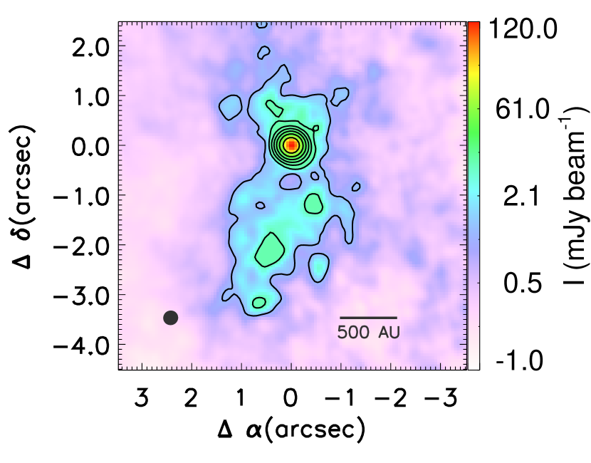
Figure 1: The 873 $\mu$m dust continuum image produced with the natural weighting and the UV taper of 0.2″. The contour levels increase by a factor of two from 5 $\sigma$ to 320 $\sigma$ (1 $\sigma$= 0.21 mJy beam^-1). The origin is the position of the continuum peak for EC 53. The ellipse on the bottom left corner represents the synthesized beam, and the scale bar of 500 AU is presented at the bottom right. Note that the color scale has two linear slopes below and above 2.1 mJy beam^-1  in order to present the extended emission.

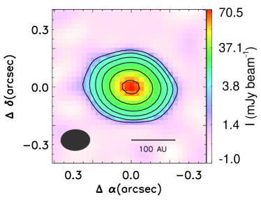
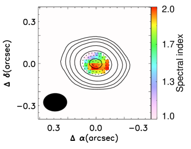
Figure 2: Left: Dust continuum images produced with the uniform weighting. The contour levels increase by a factor of two from 5 $\sigma$ to 160 $\sigma$ (1 $\sigma$= 0.38 mJy beam^-1). Note that the color scale has two linear slopes below and above 3.8 mJy beam^-1. The black ellipse on the bottom left corner indicates the beam size, and the scale bar of 100 AU is presented at the bottom right. Right: The distribution of the spectral index ($\alpha$; F${}_{\nu}\propto\nu^{\alpha}$) derived from the images produced with the uniform weighting. The solid contours are the same as those on the left panel. The dotted contours represent the 1 $\sigma$ errors of the spectral index from 0.5 (outermost) to 0.3 (innermost) with the step size of 0.1. The beam size of the image for the spectral index is presented as the black ellipse on the bottom left corner.

The 343.4 GHz (873 $\mu$m) continuum image with a lower resolution (Figure 1) shows extended emission along the north-south direction as well as a compact source. The compact source is resolved in the higher resolution image as shown on the left panel of Figure 2. The compact emission could originate from the disk (see Sections 3.2.1 and 4.1). The properties of the continuum emission are derived by fitting a Gaussian profile using the task ‘imfit’ in CASA.

The peak of the continuum emission is located at $\alpha$(J2000)= 18^h29^m51.17685^s and $\delta$(J2000)= +01^d16^m40.3892″. This peak position is consistent to within $\sim$0.2″ of the positions from Spitzer (Harvey et al., 2006; Hsieh & Lai, 2013), VLA (Ortiz-León et al., 2015), and high-resolution Keck $K_{S}$-band imaging (Hodapp et al., 2012), after applying the proper motion correction for Serpens Main of $\sim$10 mas yr^-1 towards the south-east (Ortiz-León et al., 2017; Herczeg et al., 2019). The position is offset to the north of the 2MASS (Cutri et al., 2003) and neoWISE (Cutri & et al., 2014) positions, likely a result of nebulosity seen to the south of the EC 53 binary system by Hodapp et al. (2012).

The deconvolved image of the disk shows that the major and minor axes are 144.2 $\pm$ 2.4 mas and 118.4 $\pm$ 2.2 mas with a position angle of 60.0 $\pm$ 4.2^∘. The ratio of the major and minor axes suggests the disk inclination of 34.8 $\pm$ 2.1^∘. When this position angle and the inclination are adopted, the disk radius that encircles 95% of the disk flux is 214 mas (93 AU at the distance of 436 pc), similar to the typical size of more evolved protoplanetary disks (e.g. Tripathi et al., 2017; Cieza et al., 2019; Long et al., 2019).

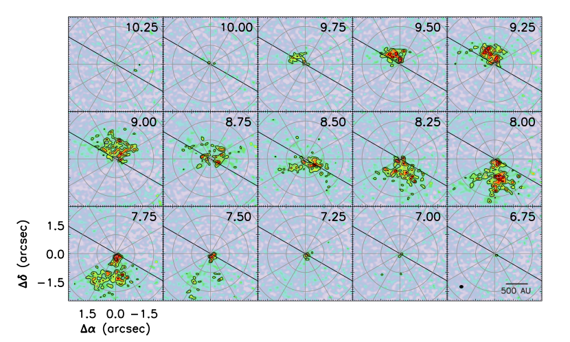
Figure 6: Velocity channel maps of C¹⁷O  3–2. The data are extracted from the briggs weighting image. The contour levels start from 4 $\sigma$ and increase in step of 2 $\sigma$ (1$\sigma$= 3.85 mJy beam^-1). The gray lines and circles are plotted in step of 30^∘  and 1.0″, respectively, to identify the position of emission clearly. The synthesized beam and the scale bar of 500 AU are presented at the bottom left and right, respectively, in the panel with the velocity of 6.75 km s^-1.

This position angle and inclination are both consistent with previous observations. The observed position angle of the disk is roughly perpendicular to the direction of the H₂ jet at 140^∘ (Herbst et al., 1997) and the ¹²CO 3–2 outflow at 135^∘ (Dionatos et al., 2010). Hodapp et al. (2012) suggested that the disk of EC 53 is seen nearly edge-on based on the cometary feature in the near-IR image. However, the inclination of the outflow axis could be lower than the half-opening angle of the outflow cavity when a protostar is observed in near-IR scattered light (Reipurth et al., 2000). Indeed, the near-IR image of EC 53 (Figure 6 in Hodapp et al., 2012, see the blue dashed curve on the bottom right panel in Figure 3) indicates that the half-opening angle of the outflow cavity is smaller than 45^∘  and the inclination is between 30^∘ and 45^∘  (see Figure 17 in Reipurth et al., 2000). The best-fit spectral energy distribution model of EC 53 also requires a small inclination of 30^∘  (Baek et al. submitted). Furthermore, for Class I sources, [Fe II] forbidden lines trace high velocity gas with a radial velocity of 100 – 200 km s^-1  (Davis et al., 2011). Near-IR spectra of EC 53 show that the 1.644 $\mu$m [Fe II] line is blue-shifted by $\sim$170 km s^-1  (S. Park et al. in prep), which implies that the inclination of the jet should be close to face-on.

The peak intensity and total flux of the disk, which are measuring by applying ‘imfit’ to the left image of Figure 2, are 69.3 $\pm$ 0.4 mJy beam^-1  and 139.7 $\pm$ 1.2 mJy, respectively. The compact emission shown in the lower resolution image (Figure 1) has the flux of 155 mJy within an aperture of 0.7″, implying that the compact emission is mostly radiated from the disk shown in the high resolution image (Figure 2). On the other hand, the total continuum flux in Figure 1 is 330 mJy. The 850 $\mu$m flux (in the beam of 14.6″) of EC 53 with the JCMT/SCUBA-2 is 960 mJy at the quiescent phase (Yoo et al., 2017), and thus, at least 60% of the continuum emission arises from an extended envelope and is resolved out in this ALMA observation.

The disk mass may be estimated from the continuum flux by

$$M_{\rm disk}=\frac{F_{\nu}d^{2}}{\kappa_{\nu}B_{\nu}(T_{\rm dust})},$$ (1)

where $F_{\nu}$ is the observed flux (139.7 $\pm$ 1.2 mJy), $d$ is the distance to EC 53, $\kappa_{\nu}$ is the dust opacity, and $B_{\nu}(T_{\rm dust})$ is the Planck function with the dust temperature of $T_{\rm dust}$. Adopting an average dust temperature of 20 K (following Andrews, 2005), a dust opacity $\kappa_{\nu}=$ 3.4 cm² g^-1 (Beckwith et al., 1990), and a gas-to-dust ratio of 100 leads to a disk mass of 0.075 $\pm$ 0.003 M_⊙. This estimate for disk mass is consistent with standard techniques but depends on highly uncertain assumptions, including the dust opacities and optical depths (see review by Williams & Cieza, 2011).

The right panel of Figure 2 shows the spectral index $\alpha$ between two continuum images produced with the uniform weighting at frequencies of $\nu_{1}$ = 348.38 GHz and $\nu_{2}$ = 337.86 GHz. The spectral index has a relation with the optical depth $\tau_{\rm 343.4GHz}$ and the power-law index of the dust opacity $\beta$ as

$$\frac{F_{\nu_{1}}}{F_{\nu_{2}}} = \left(\frac{\nu_{1}}{\nu_{2}}\right)^{\alpha}=\frac{B_{\nu_{1}}(T)(1-\exp(-\tau_{\nu_{1}}))}{B_{\nu_{2}}(T)(1-\exp(-\tau_{\nu_{2}}))},$$ (2)

$$\tau_{\nu_{i}}=\tau_{\rm 343.4GHz}\left(\frac{\nu_{i}}{\rm 343.4GHz}\right)^{\beta},$$ (3)

where $F_{\nu_{i}}$ and $\tau_{\nu_{i}}$ are the flux and optical depth at the frequency $\nu_{i}$. The spectral index at the continuum peak is 1.9 $\pm$ 0.3, which implies that either the disk is optically thick at 343.4 GHz and/or that dust grains have grown (see Section 4.1).

The JCMT/SCUBA-2 850 $\mu$m flux of EC 53 after removing the contribution of the disk implies the envelope mass is 0.86 – 1.25 M_⊙  (see Equation (1) in Jørgensen et al., 2009). The disk to envelope mass ratio, 6 – 9%, implies that EC 53 could be a late Class 0 (1 - 10%) or an early Class I source (20 – 60 %) (Jørgensen et al., 2009). This is consistent with the early Class I stage (Dunham et al., 2015) derived from the bolometric temperature ($T_{\rm bol}$= 130 K) of the SED, although a continuum radiative transfer model is needed to estimate more accurate disk and envelope masses.

3.2 Molecular lines

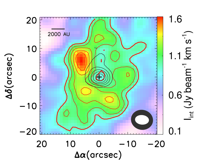
Figure 4: Integrated intensity maps for the hyperfine F₁F=01–12 line of N₂H⁺ 1–0 (image and red contour) and the C¹⁷O  3–2 (black contour) lines toward EC 53. The N₂H⁺ image is extracted from the achieve data observed by CARMA (Lee et al., 2014) and is integrated from -1.5 to +1.5 km s^-1. The lowest level and step of contours are 5 and 1 $\sigma$ (1 $\sigma$ = 0.14 Jy beam^-1 km s^-1), respectively. The black contours (10$\sigma$, 20$\sigma$, 30$\sigma$, and 40$\sigma$ RMS levels, 1$\sigma$= 132 mJy beam^-1 km s^-1) indicate the integrated intensity map of C¹⁷O  3–2 line observed with ACA (W. Park et al. in prep.). The beam sizes of CARMA and ACA are presented as the black and white ellipses on the right bottom corner, respectively. The scale bar of 2000 AU is at the top left. The N₂H⁺ molecule is depleted around EC 53 where the C¹⁷O  line emission is detected.

In this section, we infer the morphology of the circumstellar material by measuring gas kinematics in the spectral images of emission lines. The different emission lines probe the disk, infall, and outflows of the source, as described below. A source velocity of 8.5 km s^-1  is adopted throughout this analysis, based on the rotation profile of the C¹⁷O  line along the disk direction (Section 3.2.1). This value is similar to a previous measurement of $\sim$8.35 km s^-1  using N₂H⁺ 1–0 line emission measured with the CARMA (Combined Array for Research in Millimeter-wave Astronomy) data that has a beam size of 7″  (Lee et al., 2014), with a slight offset that may be explained because the N₂H⁺ species is depleted at the source position (Figure 4).

Figure 3 shows integrated intensity maps for the detected molecular lines toward EC 53. H¹³CO⁺  4–3, C¹⁷O  3–2, and CCH N= 4–3, J= 7/2–5/2, F= 4–3, F= 3–2 (in the bottom panels) consist of compact emission near the continuum peak and more extended emission while C³⁴S 8–7, CH₃OH, and other weak CCH lines (in the top panels) show only compact and weak emission near the continuum source. Those weak CH₃OH  and CCH lines are stacked individually to get a higher signal-to-noise ratio. The observed lines are listed in Table 1.

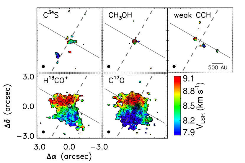
Figure 5: Integrated intensity maps (contours) and intensity weighted velocity maps (images) for the detected molecular lines toward EC 53 except for CCH. The contours are the same as Figure 3.

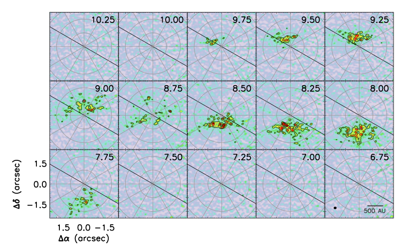
Figure 7: Same as Figure 6 except for H¹³CO⁺  4–3. The RMS noise level (1 $\sigma$) is 4.13 mJy beam^-1.

The integrated intensity maps of the H¹³CO⁺  and C¹⁷O  lines generally show similar distributions. Both lines have red-shifted and blue-shifted components in the north and south, respectively, as shown in the intensity weighted velocity map (Figure 5). The velocity channel maps of C¹⁷O  and H¹³CO⁺  (Figures 6 and 7) show that the red-shifted components (9.00 – 9.75 km s^-1) have decreasing velocity with the distance from the protostar. Such a profile is expected for red-shifted emission from infalling (accreting) material, as also seen in the Class I source L1489 IRS (Yen et al., 2014). The same trend is also observed in the C¹⁷O  blue-shifted components (8.00 – 7.25 km s^-1) near the protostar (r $<$ 1″). On the other hand, the blue-shifted velocity (8.50 – 7.75 km s^-1) increases with the distance from the protostar at r $\geq$ 1″. This implies that the blue-shifted emission at the scale of r $\geq$ 1″  traces the gas in the outflow cavity wall (e.g., Arce et al., 2013). The blue-shifted monopolar outflow could be due to an asymmetric structure of the circumstellar environment (Loinard et al., 2013).

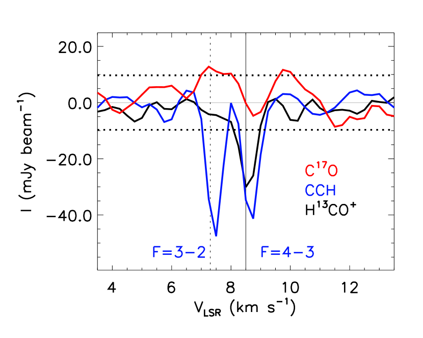
Figure 8: The spectra of H¹³CO⁺  (black), CCH (blue), and C¹⁷O  (red) at the continuum peak. The spectra are extracted from the briggs weighting images and Hanning-smoothed. The solid vertical black line indicates the source velocity (8.5 km s^-1). The dotted vertical line indicates the line center of the CCH F= 3–2. The dotted horizontal black lines show $\pm$ 3 $\sigma$ of the C¹⁷O  (1$\sigma$ = 3 mJy beam^-1).

At the continuum peak, absorption against the continuum emission is detected in the H¹³CO⁺  and strong CCH lines, while self-absorption is detected in the C¹⁷O  line (Figure 8). This deep absorption below the continuum level in the H¹³CO⁺  and strong CCH lines is red-shifted, tracing the infalling envelope material (Evans et al., 2015). The high velocity ($|\Delta V|>1$ km s^-1  from the source velocity) emission feature detected in the C¹⁷O  line (the red spectrum in Figure 8), which may trace the disk rotation, is missing in the H¹³CO⁺  line. Figure 7 shows that there is no H¹³CO⁺  line emission within $\sim$0.2″  from the protostar. The related chemistry for this phenomenon is discussed in Section 4.2.

The strong CCH line emission (the bottom right contour image of Figure 3) seems to trace the outflow cavity walls. The stream to the east, which appears distributed along the blue-shifted outflow cavity wall, is also seen in the near-IR narrow band image covering the H₂ emission (Hodapp et al., 2012). Another stream toward the north direction looks like a mirror image of the eastward stream with respect to the disk midplane (the solid gray line in Figure 3), which could imply that the northward stream might trace the red-shifted outflow cavity wall. CCH emission along the outflow cavity walls is also found in L1527, IRAS 15398-3359, and L483 (Oya et al., 2014; Sakai et al., 2014; Oya et al., 2017).

The CH₃OH  and other weak CCH lines are marginally detected (see Table 1). While the CH₃OH  lines are detected near the continuum peak, the weak CCH lines are missing toward the continuum source, instead peaking at 0.55″  from the continuum peak along the disk direction. The same phenomenon has been observed in other sources: in L1527, IRAS 15398-3359, and L483 the CCH is also depleted near the continuum peak and has strong emission off the peak (Oya et al., 2014; Sakai et al., 2014; Oya et al., 2017). The CCH molecule reacts with H₂ at warm temperatures (see e.g., Aikawa et al., 2012) and could be destroyed by those gas phase reaction in the warm and dense inner envelope and/or frozen on the dust grain in the cold and dense disk.

The C³⁴S 8–7 line seems to trace the dense molecular gas near the continuum peak as well as in the outflow cavity wall. The SiO 7–6 line was also observed but not detected.

3.2.1 Kinematics of C¹⁷O  3–2: Disk vs. Infalling rotating envelope?

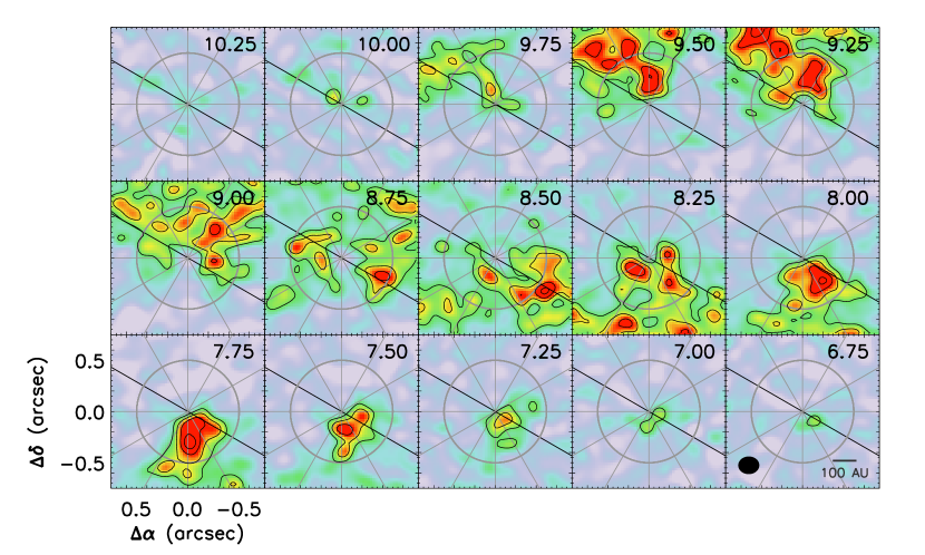
Figure 9: Zoom-in of Figure 6. The gray circle indicates the radius of 0.5″.

The rotation profile along the disk direction provides evidence of the kinematics of the disk. Figure 9 shows velocity channel maps for C¹⁷O  near the continuum peak. The innermost regions have a position-velocity distribution that would be expected for a disk. Beyond 0.5″  along the position angle of 60^∘  (the black solid line in Figure 9), the spatial distribution of red-shifted components (9.75 and 9.50 km s^-1) implies that this emission might not be associated with the disk. In the following analysis, we fit the rotation profile only within 0.5″. The highest velocity components are close to the protostar, and the models with different position angles from 30^∘  to 60^∘  do not show significant variation in the rotation profile.

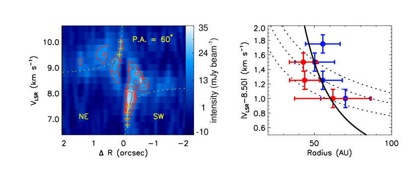
Figure 10: Position-velocity diagram (left) and rotation profile (right) of C¹⁷O  3–2 along the disk direction with a position angle of 60 ^∘. Left: The image and red contours indicate the observed C¹⁷O  intensity extracted from the briggs weighting image. The contours start from 4 $\sigma$ in step of 1 $\sigma$ (1$\sigma$= 3.8 mJy beam^-1). The dashed yellow lines represent the Keplerian motion with a protostellar mass of 0.3 M_⊙. Right: The red (blue) points indicate the peak positions along given red-shifted (blue-shifted) velocity channels as shown in the yellow cross in the left panel. Three dotted lines represent the Keplerian motion with a protostellar mass of 0.4 (top), 0.3 (middle), and 0.2 M_⊙  (bottom), respectively. When these data are fit with a power-law function, the power law index is -2.1 $\pm$ 2.2 (black solid line).

Figure 10 shows the position-velocity diagram along the disk (left) and the rotation velocity profiles (right) of EC 53. The power-law index that fits the velocity profile is -2.1 $\pm$ 2.2. If the highest blue-shifted point is excluded, the best-fit power law is -1.1 $\pm$ 0.7, indicative of the rotating infalling envelope under the constraint of angular momentum conservation (Sakai et al., 2014). However, our current observation with large scatter and a low signal-to-noise ratio cannot rule out a rotational profile produced by the Keplerian disk. The range of the rotation velocity corresponds to the Keplerian motions with the protostellar masses of 0.2 and 0.4 M_⊙  when we adopted the inclination of 35^∘. Since the protostar is still young and the envelope massive, the present-day protostellar mass may be much lower than the final mass after stellar assembly is complete.

4 Discussion

4.1 Dust grain growth

The observed 873 $\mu$m continuum emission is mainly from dust thermal emission. In the continuum images produced with uniform weighting, the peak intensity and the spectral index at the continuum peak are 69.3 $\pm$ 0.4 mJy beam^-1  and 1.9 $\pm$ 0.3, respectively. The spectral index lower than 2 cannot be explained by non-thermal emission, since VLA 4.5 and 7.5 GHz observations (with a beam size of $\sim$0.4″, Ortiz-León et al., 2015) indicate that the 873 $\mu$m flux from the non-thermal emission is lower than 0.2 mJy. Therefore, the spectral index of 1.9 $\pm$ 0.3 implies that the continuum emission is optically thick and/or that the power-law index of dust opacity is lower than 1 in the isothermal condition.

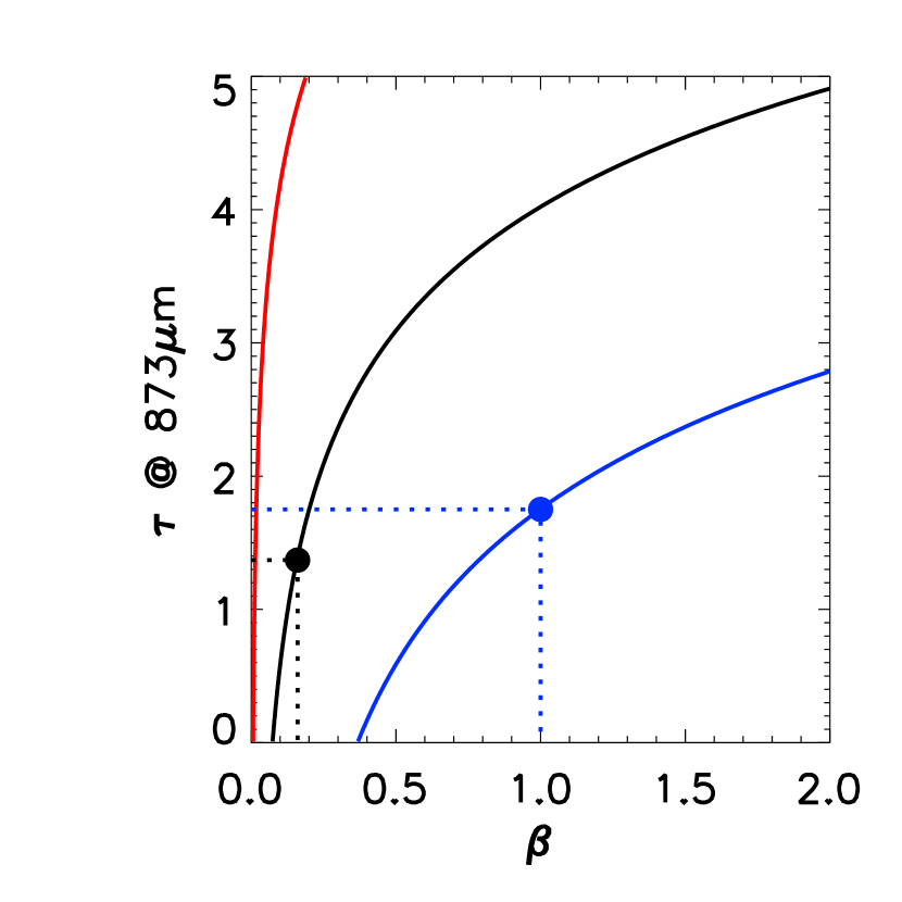
Figure 11: The optical depth at 873 $\mu$m ($\tau$) and the power-law index of dust opacity ($\beta$) producing the spectral index ($\alpha$)of 1.9 for the given dust temperatures: 20 (blue), 50 (black), and 80 K (red), respectively. The blue circle indicates the $\tau$ producing $\alpha$=1.9 for the temperature of 20 K and $\beta$=1 used to calculate the disk mass (Section 3.1) while the black circle indicates the $\beta$ producing $\alpha$=1.9 for the temperature of 50 K and $\tau$=1.4

The sub-mm continuum spectral index can be used to derive the properties of emitting sources and dust grains. The low spectral index (1.9 $\pm$ 0.3) for the dust continuum emission indicates that the compact continuum emission could be emitted from the disk. On the other hand, the spectral index derived from the ACA (Atacama Compact Array) images of EC 53 in band 6 and 7, which trace the envelope of EC 53, is about 2.5 (W. Park, in prep.). Continuum emission images at 1.1 mm and 3 mm toward two Class I sources Elias 29 and WL 12 show that the spectral indices in the disk are typically lower than 2, while in the envelope are typically higher than 2.5 (Miotello et al., 2014). Figure 11 shows the optical depth and the power-law index of dust opacity, $\beta$, for given dust temperatures reproducing the observed spectral index of 1.9 $\pm$ 0.3. When we adopt the dust temperature of 20 K and $\beta$= 1, which are used for the calculation of the disk mass, the average optical depth of dust continuum is 1.8${}_{-1.0}^{+2.2}$ (see the blue circle in Figure 11). If this optical depth is considered, the disk mass derived by Equation (1) is smaller than the actual value by a factor of two. On the other hand, if we know the dust temperature and the optical depth of dust continuum, then we can derive $\beta$, which constrains the dust properties; grain growth in the disk reduces the power-law index of dust opacity (e.g., Natta et al., 2007).

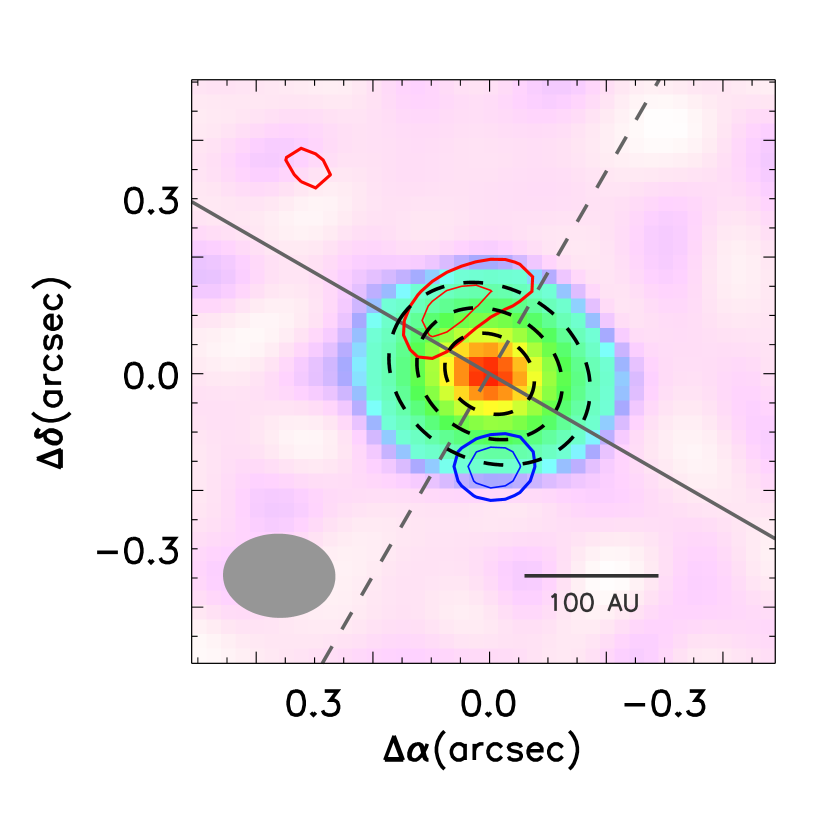
Figure 12: The C¹⁷O  3–2 integrated intensity map (contour) of EC 53 produced by the uniform weighting. The red and blue contours indicate the red- and blue-shifted components, respectively, integrated over the velocity from 1.0 to 1.5 km s^-1  with respect to the source velocity. The lowest contour and subsequent contour step are 5 $\sigma$ and 1 $\sigma$, respectively (1 $\sigma$= 3.5 mJy beam^-1 km s^-1). The background image is the dust continuum intensity as in the left panel of Figure 2. Three dashed ellipses correspond to the radii of 0.08, 0.13, and 0.18″, respectively. The beam size and 100 AU scale bar are shown in the bottom left and right corners, respectively.

The optical depth of the dust continuum can be derived from a molecular line. As shown in the integrated intensity maps for the detected molecular lines (Figure 3), the emission peaks of all the molecular lines are off the continuum peak. Figure 12 shows the C¹⁷O  3–2 intensity map integrated over the velocity from 1.0 to 1.5 km s^-1  with respect to the source velocity. This integrated intensity map was produced using the uniform weighting to trace how the C¹⁷O  emission is distributed near the continuum peak, by excluding the contribution of the extended emission. The C¹⁷O  line emission is clearly depleted near the continuum peak and peaks around 0.13″  from the continuum peak. This phenomenon was also observed in TMC 1A (Harsono et al., 2018) and V883 Ori (Lee et al., 2019). A high optical depth and strong emission of the dust continuum can reduce the intensity of the molecular line emission; the observed line intensity is reduced by $\exp(-\tau_{c})$ with the dust optical depth of $\tau_{c}$ (Yen et al., 2016; Lee et al., 2019).

We adopt a simple thin disk with power-law distributions for the continuum optical depth $\tau_{c}(r)$ and the dust temperature $T_{\rm dust}(r)$:

$$\tau_{c}(r) = \tau_{\rm 0.1}\left(\frac{r}{0.1\arcsec}\right)^{-\psi},$$ (4)

$$T_{\rm dust}(r) = T_{\rm 0.1}\sqrt{\frac{0.1\arcsec}{r}},$$ (5)

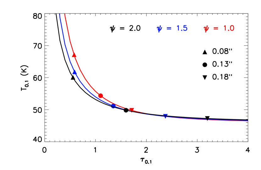
Figure 13: Model parameters producing the C¹⁷O  emission distribution shown in Figure 12. The lines indicate the continuum optical depth ($\tau_{\rm 0.1}$) and the dust temperature ($T_{\rm 0.1}$) at 0.1″  which reproduce the continuum intensity (69.3 $\pm$ 0.4 mJy beam^-1) at the continuum peak. Different colors indicate different power-law indices of optical depth (see Equation (4)). The upward triangles, circles, and downward triangles indicate the model parameters producing the C¹⁷O  emission peak at 0.08″, 0.13″, and 0.18″, respectively, which are marked by the dashed ellipses in Figure 12.

where $\tau_{\rm 0.1}$ and $T_{\rm 0.1}$ are the continuum optical depth and dust temperature at 0.1″. We test three power-law indices of optical depth: $\psi$= 1.0, 1.5, and 2.0. The solid lines in Figure 13 indicate the models producing the observed 873 $\mu$m intensity at the continuum peak (69.3 $\pm$ 0.4 mJy beam^-1). The emission from the inclined thin disk (inclination= 35^∘) are convolved with the observed beam.

The C¹⁷O  intensity within 0.5″  (Figure 9) is lower than 45 mJy beam^-1, which corresponds to a brightness temperature ($T_{\rm b}$) of $\sim 14$ K. If the gas and dust have the same temperature, the C¹⁷O  brightness temperature is about two times lower than the gas temperature, indicating that the C¹⁷O  line is optically thin. When we assume that the column density ratio of C¹⁷O  and dust is spatially constant, and the C¹⁷O  molecules are in the local thermal equilibrium (LTE) condition, the above thin disk model produces the C¹⁷O  emission distribution $I(r)$:

$$I(r)\propto\tau_{c}(r)\cdot n_{u}\left(T_{\rm dust}(r)\right)\cdot\exp\left(-\tau_{c}(r)\right),$$ (6)

where the upper level population $n_{u}(r)$ is derived from the Boltzmann distribution with $T_{\rm dust}(r)$. In the right hand side of Equation (6), the first term ($\tau_{c}(r)$) represents the total column density of C¹⁷O, the second term ($n_{u}\left(T_{\rm dust}(r)\right)$) is the fraction of C¹⁷O  to produce the C¹⁷O  3–2 line, and the third term indicates the extinction of the line by dust grains.

Our models with the dust temperature of 50 – 55 K and dust optical depth of 1.1 – 1.6 at the radius of 0.1″  can reproduce the C¹⁷O  emission peak around 0.13″  (see the circles in Figure 13 and Table 2). The thin dust disk with a truncated radius of 0.13″  can reproduce the observed continuum flux of 139.7 mJy as well as the disk size measured with ‘imfit’. The entire dust disk is optically thick, and thus, the C¹⁷O  emission peaks at the dust disk radius. When the dust opacity of 3.4 cm² g^-1 at 343.4 GHz (Beckwith et al., 1990) and gas-to-dust ratio of 100 are adopted, the models show the disk mass is 0.1 M_⊙  with an uncertainty by a factor of two, which is similar to the disk mass of 0.075 M_⊙ (see Section 3.1). Note that grain growth can change the dust opacity (e.g., Ricci et al., 2010), and thus, the disk mass. The calculated dust mass would also be 3.3 times lower if we use $50$ K instead of $20$ K for the average dust temperature in the disk.

For the dust temperature of $\sim$50 K and the continuum optical depth of $\sim$1.4 near the continuum peak in our model, the power-law index of the dust opacity ($\beta$) must be lower than 0.2 $\pm$ 0.6 to reproduce the observed spectral index of 1.9 $\pm$ 0.3 (see the black circle in Figure 11). This suggests that the maximum size of dust grains should be larger than centimeter sizes (e.g., Ricci et al., 2010; Testi et al., 2014). The large disk mass of about 0.1 M_⊙  and the large grain size imply a possibility of planet formation even in the early evolutionary stage, as argued by Harsono et al. (2018).

4.2 Water and CO snowlines

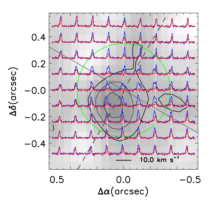
Figure 14: The spectral maps of C¹⁷O  (blue) and H¹³CO⁺  (red) on top of the CH₃OH  integrated intensity map (image and contour). The contour levels are the same as those in Figure 5. The horizontal bar on the bottom indicates the scale of the x-axis (velocity range from -5 to 5 km s^-1). The horizontal and vertical white lines indicate the continuum level and the source velocity, respectively. The green circle indicates the radius of 0.35″  (153 AU at the distance of 436 pc).

Figure 14 shows the spectral maps of H¹³CO⁺  and C¹⁷O  on top of the image of the CH₃OH  integrated intensity map. Outside of the CH₃OH  emission area, the H¹³CO⁺  line has a similar intensity to the C¹⁷O  line. However, the H¹³CO⁺  line emission is depleted near the continuum peak, where the methanol lines emit. On the other hand, the C¹⁷O  line is still strong and broad near the continuum peak where the H¹³CO⁺  emission completely disappears. The CH₃OH  line might emit from the disk or infalling rotating inner envelope traced by C¹⁷O  because the CH₃OH  line has a similar line width to that of the C¹⁷O  line. The emission peak of CH₃OH  is offset from the continuum peak probably due to the optically thick continuum emission, as also shown in the C¹⁷O  emission distribution. The anti-correlation between the H¹³CO⁺  and CH₃OH  emission was also detected in IRAS 15398-3359 and may be caused by the destruction of H¹³CO⁺  by water, which evaporates simultaneously with CH₃OH  (Jørgensen et al., 2013). The methanol emission is known to be related closely with water emission (Bjerkeli et al., 2016). However, the observed CH₃OH  emission is extended up to $\sim$0.35″  (see Figure 14), which is an order of magnitude larger than the water snow line expected from the current luminosity. In the thin disk model described above, the water snow line (100 K) is located around 0.03″.

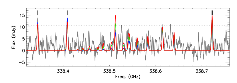
Figure 15: The methanol spectra for EC 53. The gray line shows the observed spectra extracted with the aperture of 0.6″. The spectra are smoothed with the boxcar of 1.8 km s^-1. The black dotted line indicates the 5 $\sigma$ level (1 $\sigma$= 2.1 mJy). The four vertical black bars indicate the marginally detected CH₃OH  lines presented in Table 1. The red, green, and blue lines show the model spectra with the temperatures of 70, 50, and 30 K and with the methanol column densities of 5.2, 3.7, and 2.2 $\times 10^{15}$cm^-2, respectively.

To measure the abundance of methanol, we first extracted the CH₃OH  spectra with an aperture of 0.6″. We then reproduced this spectrum with a simple LTE model using molecular data from the Cologne Database for Molecular Spectroscopy (CDMS, Müller et al., 2001). The model includes the dust continuum and opacity and assumes a line width of 2 km s^-1. The molecular hydrogen column density of $\sim$10²⁵ cm^-2 is estimated from the dust continuum flux measured with the same 0.6″  aperture when the dust opacity of 3.4 cm² g^-1 (Beckwith et al., 1990), gas-to-dust ratio of 100, and the dust temperatures of 30, 50, and 70 K are adopted. The derived methanol column density and abundance are $\sim$10¹⁵ cm^-2 and $\sim$10^-10, respectively (see Figure 15).

The methanol emission from the much larger outburst of V883 Ori provides a useful comparison for that from EC 53. The derived methanol abundance for EC 53 is two orders of magnitude lower than the CH₃OH  abundance of $\sim$10^-8 for V883 Ori (Lee et al., 2019) although the physical size of the methanol emission regions are similar for V883 Ori and EC 53. In both cases, the methanol abundance may be underestimated by an order of magnitude because of the optical depths of dust continuum and methanol itself (van ’t Hoff et al., 2018; Lee et al., 2019).

The difference in abundance between EC 53 and V883 Ori, despite the similar size of methanol emission, might be related to the repeated outbursts and the 2-D structure of the sublimation region. The water/methanol sublimation occurs over the 2-D structure in the disk (van ’t Hoff et al., 2018; Lee et al., 2019); the snow line extends to much larger radii at the disk surface than at the disk midplane. During the quiescent phase, the methanol freezes back onto grain surfaces very efficiently in the disk midplane but much more slowly at the disk surface, where the density is much lower. As a result, if there were powerful burst events in the past in EC 53, the surface snow line could be very large, despite a much smaller snow line at the disk midplane because of the low current luminosity. This will make the derived abundance of gaseous CH₃OH  low compared to the size of emission in EC 53. In contrast, V883 Ori has an ongoing outburst with the luminosity greater than that of EC 53 in the quiescent phase by two orders of magnitude. As a result, the snow line is large even at the disk midplane, resulting in the higher abundance of gaseous methanol in V883 Ori.

In summary, the different timescales for freeze-out between the disk midplane and surface may explain why the methanol emission region extends far beyond the location of the water snow line expected from the current luminosity of EC 53, despite the low overall abundance compared with V883 Ori. The repeated accretion bursts in EC 53 may extend the water snow line, and the disk surface will retain the larger snow line for a longer time than the disk midplane.

Grain growth in the disk midplane could also contribute to increasing the radius of the snow line in the disk midplane. When the ratio of scale height to radius is 0.1, the density at the midplane near 0.1″  is $\sim 10^{11}$cm^-3. If we adopt the typical ISM grain size (0.1 $\mu$m) and the typical abundance of the dust grain with respect to the molecular hydrogen ($\sim 10^{-12}$), then all methanol molecules freeze out onto the dust grain within a few days (Lee et al., 2004). However, the freeze-out timescale could be longer than a few years when the maximum grain size is larger than 1 cm (see Section 4.1), since the total surface area of grains would then be reduced by a factor of $\sim$300, assuming that the total grain mass is conserved, and the minimum size of grain and the power-law index of grain size distribution are 0.1 $\mu$m and -3.5, respectively. This freeze-out timescale is longer than the periodicity of 1.5 years in the accretion onto EC 53 (Yoo et al., 2017). The CH₃OH  emission could trace the water snow line constructed during the burst phase of the period, when the luminosity is four times brighter (Yoo et al., 2017) and the water snow line would then be two times larger, or $\sim$0.06 ″  (Min et al., 2011; Jørgensen et al., 2015; Visser et al., 2015). Although the CH₃OH  emission could extend further than 0.06″  at the disk surface because of the high temperature and low density in the irradiated disk (van ’t Hoff et al., 2018; Lee et al., 2019), the measured size of the CH₃OH  emission requires a more extreme (factor of $\sim$100) luminosity enhancement.

Figure 4 shows that the N₂H⁺ line emission is anti-correlated with the C¹⁷O  3–2 line emission. It is hard to determine accurately the size of the N₂H⁺ emission hole because of the low spatial resolution ($\sim$7″) of CARMA. However, our C¹⁷O  ALMA data (Figures 3 and 6) indicate that the C¹⁷O  line extends to $\sim$2″  along the disk midplane direction. In addition, in the ACA observation (Figure 4), the full width at half maximum of the C¹⁷O  3–2 emission is about 2.7″. This observed CO snow line ($\sim$1000 AU) is also larger than that expected from the luminosities both for the quiescent and burst phases ($\sim$250 AU and $\sim$500 AU, respectively). These CO sublimation radii (25 K) are derived from the spectral energy distribution modelings of EC 53 (G. Baek et al. submitted.). Together, the estimated sizes of the C¹⁷O  emission and the N₂H⁺ emission hole support suggestion of repeated and/or more extreme bust events in the past.

5 Summary

We carried out high resolution ALMA observations toward EC 53. The main results are:

1) The continuum image at 873 $\mu$m shows that EC 53 has a massive disk (0.075 $\pm$ 0.003 M_⊙) with centimeter-size grains, implying that a planet could form even in the early evolutionary stage to induce the observed periodic variation of accretion rate. Furthermore, the optically thick dust continuum emission in the sub-mm reduces the molecular line emission near the continuum peak.

(2) The high velocity components of C¹⁷O  3–2 show a rotation feature along the disk direction, however, the current observation cannot constrain whether the rotation profile is associated with the Keplerian disk and/or an infalling envelope. If the Keplerian motion is adopted, the rotation profile indicates that EC 53 has a protostellar mass of $\sim$0.3 $\pm$ 0.1  M_⊙.

(3) The anti-correlation of CH₃OH  and H¹³CO⁺  near the continuum peak could be associated with the destruction of H¹³CO⁺  by evaporated water molecules.

(4) The observed methanol and CO emissions are more extended than the snow lines expected due to the current luminosity, implying repeated and/or more extreme accretion burst events in the past. The luminosity and therefore the abundance of CH₃OH is two orders of magnitude lower than measured from disks undergoing larger outbursts, perhaps because the CH₃OH is frozen out at the disk midplane but is still in the gas phase in the lower-density disk surface.

Table 1: Detected molecular lines

Molecule	Frequency (GHz)	Transition	log10 Aa (s-1)	E${}_{\rm up}^{b}$ (K)	g${}_{\rm up}^{c}$
C 17O	337.060988d	J= 3–2	-5.63433	32.4	12
C34S	337.396459	J= 7–6	-3.11804	50.2	15
CH3OH	338.3446280e	7(-1,7)–6(-1,6)	-3.77817	70.5	15
	338.4086810e	7(0,7)–6(0,6)++	-3.76902	65.0	15
	338.7216300e	7(2,6)–6(2,5)	-3.80441	90.9	15
	338.7229400e	7(-2,6)–6(-2,5)	-3.80441	90.9	15
H13CO+	346.9983440	J= 4–3	-2.48309	41.6	9
CCH	349.3992756f	N= 4–3, J= 7/2–5/2, F= 4–3	-3.90313	41.9	9
	349.4006712f	N= 4–3, J= 7/2–5/2, F= 3–2	-3.92139	41.9	7
	349.4146425e,g	N= 4–3, J= 7/2–5/2, F= 3–3	-5.15397	41.9	7
	349.6036139e,g	N= 4–3, J= 7/2–7/2, F= 4–4	-5.28599	41.9	9

Note. — The molecular information is adopted from CDMS database (Müller et al., 2001).

Table 2: Thin disk model for the Continuum emission

$\psi^{a}$		1.0	1.5	2.0
$T_{\rm 0.1}^{a}$	(K)	52	50	49
$\tau_{\rm 0.1}^{a}$		1.1	1.4	1.6
$r_{\rm max}^{b}$	(″)	0.14	0.13	0.13
$T_{\rm med}^{c}$	(K)	53	51	50
$M_{\rm disk}^{d}$	(M⊙)	0.05	0.10	0.23

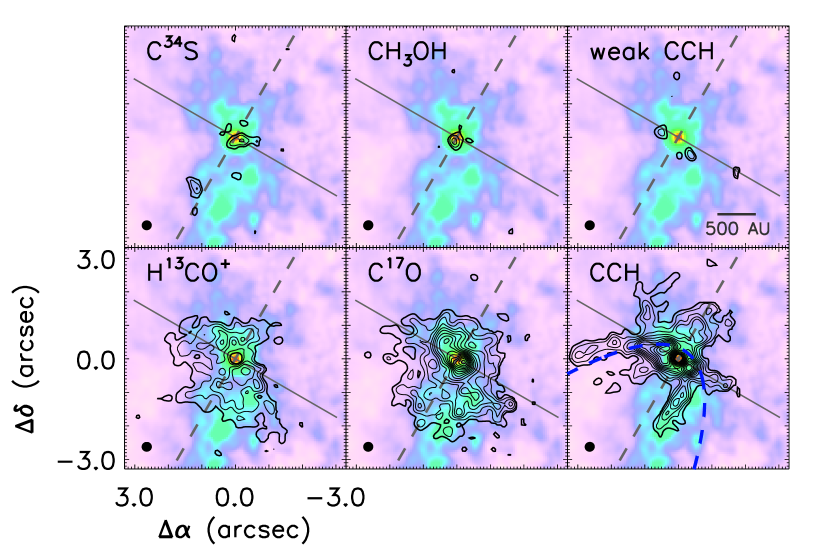
Figure 3: Integrated intensity maps for the detected molecular lines toward EC 53. The background image is the zoom-in of Figure 1. The thick solid and dashed gray lines indicate the disk and outflow directions, respectively. The blue dashed curvature in the bottom right panel indicates the outflow cavity wall traced by a near-IR observation (Hodapp et al., 2012). The ellipses on the bottom left corner represent the synthesized beam. The scale bar of 500 AU is at the bottom right of the weak CCH map. The CH₃OH  and weak CCH lines are marginally detected (see Table 1). Those lines of the individual molecules are stacked in order to get a higher signal-to-noise ratio. The 1 $\sigma$ RMS noise, the lowest contour, and subsequent contour step for the individual molecules are as follow: 4.7 mJy beam^-1 km s^-1, 3 $\sigma$, and 1 $\sigma$ for C³⁴S, 2.7 mJy beam^-1 km s^-1, 3 $\sigma$, and 1 $\sigma$ for CH₃OH, 4.4 mJy beam^-1 km s^-1, 3 $\sigma$, and 1 $\sigma$ for weak CCH, 4.6 mJy beam^-1 km s^-1, 5 $\sigma$, and 2 $\sigma$ for H¹³CO⁺, 4.3 mJy beam^-1 km s^-1, 5 $\sigma$, and 3 $\sigma$ for C¹⁷O, 5.6 mJy beam^-1 km s^-1, 5 $\sigma$, and 3 $\sigma$ for CCH.

derived from the thin disk model (see Table 2).

References

- Aikawa et al. (2012) Aikawa, Y., Wakelam, V., Hersant, F., Garrod, R. T., & Herbst, E. 2012, ApJ, 760, 40
- Andrews (2005) Andrews, S. M. 2005, in Protostars and Planets V Posters, 8203
- Arce et al. (2013) Arce, H. G., Mardones, D., Corder, S. A., et al. 2013, ApJ, 774, 39
- Armitage (1995) Armitage, P. J. 1995, MNRAS, 274, 1242
- Armitage (2016) —. 2016, ApJ, 833, L15
- Aspin & Reipurth (2000) Aspin, C., & Reipurth, B. 2000, MNRAS, 311, 522
- Audard et al. (2014) Audard, M., Ábrahám, P., Dunham, M. M., et al. 2014, Protostars and Planets VI, 387
- Bae et al. (2014) Bae, J., Hartmann, L., Zhu, Z., & Nelson, R. P. 2014, ApJ, 795, 61
- Beckwith et al. (1990) Beckwith, S. V. W., Sargent, A. I., Chini, R. S., & Guesten, R. 1990, AJ, 99, 924
- Bell & Lin (1994) Bell, K. R., & Lin, D. N. C. 1994, ApJ, 427, 987
- Bjerkeli et al. (2016) Bjerkeli, P., Jørgensen, J. K., Bergin, E. A., et al. 2016, A&A, 595, A39
- Bonnell & Bastien (1992) Bonnell, I., & Bastien, P. 1992, ApJ, 401, L31
- Cieza et al. (2019) Cieza, L. A., Ruíz-Rodríguez, D., Hales, A., et al. 2019, MNRAS, 482, 698
- Contreras Peña et al. (2019) Contreras Peña, C., Naylor, T., & Morrell, S. 2019, MNRAS, 486, 4590
- Contreras Peña et al. (2017) Contreras Peña, C., Lucas, P. W., Minniti, D., et al. 2017, MNRAS, 465, 3011
- Cutri & et al. (2014) Cutri, R. M., & et al. 2014, VizieR Online Data Catalog, II/328
- Cutri et al. (2003) Cutri, R. M., Skrutskie, M. F., van Dyk, S., et al. 2003, VizieR Online Data Catalog, II/246
- D’Angelo & Spruit (2012) D’Angelo, C. R., & Spruit, H. C. 2012, MNRAS, 420, 416
- Davis et al. (2011) Davis, C. J., Cervantes, B., Nisini, B., et al. 2011, A&A, 528, A3
- Dionatos et al. (2010) Dionatos, O., Nisini, B., Codella, C., & Giannini, T. 2010, A&A, 523, A29
- Dunham et al. (2010) Dunham, M. M., Evans, II, N. J., Terebey, S., Dullemond, C. P., & Young, C. H. 2010, ApJ, 710, 470
- Dunham et al. (2015) Dunham, M. M., Allen, L. E., Evans, II, N. J., et al. 2015, ApJS, 220, 11
- Eiroa & Casali (1992) Eiroa, C., & Casali, M. M. 1992, A&A, 262, 468
- Enoch et al. (2009) Enoch, M. L., Evans, II, N. J., Sargent, A. I., & Glenn, J. 2009, ApJ, 692, 973
- Evans et al. (2015) Evans, Neal J., I., Di Francesco, J., Lee, J.-E., et al. 2015, ApJ, 814, 22
- Evans et al. (2009) Evans, II, N. J., Dunham, M. M., Jørgensen, J. K., et al. 2009, ApJS, 181, 321
- Fischer et al. (2017) Fischer, W. J., Megeath, S. T., Furlan, E., et al. 2017, ApJ, 840, 69
- Gutermuth et al. (2009) Gutermuth, R. A., Megeath, S. T., Myers, P. C., et al. 2009, ApJS, 184, 18
- Harsono et al. (2018) Harsono, D., Bjerkeli, P., van der Wiel, M. H. D., et al. 2018, Nature Astronomy, 2, 646
- Hartmann et al. (2016) Hartmann, L., Herczeg, G., & Calvet, N. 2016, ARA&A, 54, 135
- Harvey et al. (2006) Harvey, P. M., Chapman, N., Lai, S.-P., et al. 2006, ApJ, 644, 307
- Herbig (1977) Herbig, G. H. 1977, ApJ, 217, 693
- Herbig (2008) —. 2008, AJ, 135, 637
- Herbst et al. (1997) Herbst, T. M., Beckwith, S. V. W., & Robberto, M. 1997, ApJ, 486, L59
- Herczeg et al. (2017) Herczeg, G. J., Johnstone, D., Mairs, S., et al. 2017, ApJ, 849, 43
- Herczeg et al. (2019) Herczeg, G. J., Kuhn, M. A., Zhou, X., et al. 2019, ApJ, 878, 111
- Hillenbrand & Findeisen (2015) Hillenbrand, L. A., & Findeisen, K. P. 2015, ApJ, 808, 68
- Hodapp (1999) Hodapp, K. W. 1999, AJ, 118, 1338
- Hodapp et al. (2012) Hodapp, K. W., Chini, R., Watermann, R., & Lemke, R. 2012, ApJ, 744, 56
- Hsieh & Lai (2013) Hsieh, T.-H., & Lai, S.-P. 2013, ApJS, 205, 5
- Hunter et al. (2017) Hunter, T. R., Brogan, C. L., MacLeod, G., et al. 2017, ApJ, 837, L29
- Johnstone et al. (2013) Johnstone, D., Hendricks, B., Herczeg, G. J., & Bruderer, S. 2013, ApJ, 765, 133
- Johnstone et al. (2018) Johnstone, D., Herczeg, G. J., Mairs, S., et al. 2018, ApJ, 854, 31
- Jørgensen et al. (2009) Jørgensen, J. K., van Dishoeck, E. F., Visser, R., et al. 2009, A&A, 507, 861
- Jørgensen et al. (2015) Jørgensen, J. K., Visser, R., Williams, J. P., & Bergin, E. A. 2015, A&A, 579, A23
- Jørgensen et al. (2013) Jørgensen, J. K., Visser, R., Sakai, N., et al. 2013, ApJ, 779, L22
- Kenyon et al. (1990) Kenyon, S. J., Hartmann, L. W., Strom, K. M., & Strom, S. E. 1990, AJ, 99, 869
- Kim et al. (2012) Kim, H. J., Evans, II, N. J., Dunham, M. M., Lee, J.-E., & Pontoppidan, K. M. 2012, ApJ, 758, 38
- Kospal et al. (2008) Kospal, A., Nemeth, P., Abraham, P., et al. 2008, Information Bulletin on Variable Stars, 5819
- Lee (2007) Lee, J.-E. 2007, Journal of Korean Astronomical Society, 40, 83
- Lee et al. (2004) Lee, J.-E., Bergin, E. A., & Evans, II, N. J. 2004, ApJ, 617, 360
- Lee et al. (2019) Lee, J.-E., Lee, S., Baek, G., et al. 2019, Nature Astronomy, arXiv:1809.00353
- Lee et al. (2014) Lee, K. I., Fernández-López, M., Storm, S., et al. 2014, ApJ, 797, 76
- Liu et al. (2018) Liu, S.-Y., Su, Y.-N., Zinchenko, I., Wang, K.-S., & Wang, Y. 2018, ApJ, 863, L12
- Lodato & Clarke (2004) Lodato, G., & Clarke, C. J. 2004, MNRAS, 353, 841
- Loinard et al. (2013) Loinard, L., Zapata, L. A., Rodríguez, L. F., et al. 2013, MNRAS, 430, L10
- Long et al. (2019) Long, F., Herczeg, G. J., Harsono, D., et al. 2019, ApJ, 882, 49
- Lorenzetti et al. (2012) Lorenzetti, D., Antoniucci, S., Giannini, T., et al. 2012, ApJ, 749, 188
- Mairs et al. (2017) Mairs, S., Johnstone, D., Kirk, H., et al. 2017, ApJ, 849, 107
- Masunaga & Inutsuka (2000) Masunaga, H., & Inutsuka, S.-i. 2000, ApJ, 531, 350
- McMullin et al. (2007) McMullin, J. P., Waters, B., Schiebel, D., Young, W., & Golap, K. 2007, in Astronomical Society of the Pacific Conference Series, Vol. 376, Astronomical Data Analysis Software and Systems XVI, ed. R. A. Shaw, F. Hill, & D. J. Bell, 127
- Min et al. (2011) Min, M., Dullemond, C. P., Kama, M., & Dominik, C. 2011, Icarus, 212, 416
- Miotello et al. (2014) Miotello, A., Testi, L., Lodato, G., et al. 2014, A&A, 567, A32
- Müller et al. (2001) Müller, H. S. P., Thorwirth, S., Roth, D. A., & Winnewisser, G. 2001, A&A, 370, L49
- Natta et al. (2007) Natta, A., Testi, L., Calvet, N., et al. 2007, Protostars and Planets V, 767
- Nayakshin & Lodato (2012) Nayakshin, S., & Lodato, G. 2012, MNRAS, 426, 70
- Ortiz-León et al. (2015) Ortiz-León, G. N., Loinard, L., Mioduszewski, A. J., et al. 2015, ApJ, 805, 9
- Ortiz-León et al. (2017) Ortiz-León, G. N., Dzib, S. A., Kounkel, M. A., et al. 2017, ApJ, 834, 143
- Oya et al. (2014) Oya, Y., Sakai, N., Sakai, T., et al. 2014, ApJ, 795, 152
- Oya et al. (2017) Oya, Y., Sakai, N., Watanabe, Y., et al. 2017, ApJ, 837, 174
- Plunkett et al. (2015) Plunkett, A. L., Arce, H. G., Mardones, D., et al. 2015, Nature, 527, 70
- Reipurth et al. (2000) Reipurth, B., Yu, K. C., Heathcote, S., Bally, J., & Rodríguez, L. F. 2000, AJ, 120, 1449
- Ricci et al. (2010) Ricci, L., Testi, L., Natta, A., et al. 2010, A&A, 512, A15
- Safron et al. (2015) Safron, E. J., Fischer, W. J., Megeath, S. T., et al. 2015, ApJ, 800, L5
- Sakai et al. (2014) Sakai, N., Sakai, T., Hirota, T., et al. 2014, Nature, 507, 78
- Shu (1977) Shu, F. H. 1977, ApJ, 214, 488
- Testi et al. (2014) Testi, L., Birnstiel, T., Ricci, L., et al. 2014, Protostars and Planets VI, 339
- Tripathi et al. (2017) Tripathi, A., Andrews, S. M., Birnstiel, T., & Wilner, D. J. 2017, ApJ, 845, 44
- van ’t Hoff et al. (2018) van ’t Hoff, M. L. R., Tobin, J. J., Trapman, L., et al. 2018, ApJ, 864, L23
- Visser et al. (2015) Visser, R., Bergin, E. A., & Jørgensen, J. K. 2015, A&A, 577, A102
- Vorobyov & Basu (2005) Vorobyov, E. I., & Basu, S. 2005, ApJ, 633, L137
- Vorobyov & Basu (2010) —. 2010, ApJ, 719, 1896
- Williams & Cieza (2011) Williams, J. P., & Cieza, L. A. 2011, ARA&A, 49, 67
- Yen et al. (2016) Yen, H.-W., Liu, H. B., Gu, P.-G., et al. 2016, ApJ, 820, L25
- Yen et al. (2014) Yen, H.-W., Takakuwa, S., Ohashi, N., et al. 2014, ApJ, 793, 1
- Yoo et al. (2017) Yoo, H., Lee, J.-E., Mairs, S., et al. 2017, ApJ, 849, 69
- Zhu et al. (2009) Zhu, Z., Hartmann, L., Gammie, C., & McKinney, J. C. 2009, ApJ, 701, 620