SparseTrain: Leveraging Dynamic Sparsity in Training DNNs on General-Purpose SIMD Processors

Abstract.

Our community has greatly improved the efficiency of deep learning applications, including by exploiting sparsity in inputs. Most of that work, though, is for inference, where weight sparsity is known statically, and/or for specialized hardware. We propose a scheme to leverage dynamic sparsity during training. In particular, we exploit zeros introduced by the ReLU activation function to both feature maps and their gradients. This is challenging because the sparsity degree is moderate and the locations of zeros change over time. We also rely purely on software.

We identify zeros in a dense data representation without transforming the data, and performs conventional vectorized computation. Variations of the scheme are applicable to all major components of training: forward propagation, backward propagation by inputs, and backward propagation by weights. Our method significantly outperforms a highly-optimized dense direct convolution on several popular deep neural networks. At realistic sparsity, we speed up the training of the non-initial convolutional layers in VGG16, ResNet-34, ResNet-50, and Fixup ResNet-50 by 2.19x, 1.37x, 1.31x, and 1.51x respectively on an Intel Skylake-X CPU.

1. Introduction

Deep Neural Networks (DNNs) have become ubiquitous, achieving state-of-the-art results across a range of tasks from image recognition (Krizhevsky et al., [n. d.]) to speech recognition (Amodei et al., 2015) to scene generation (Radford et al., 2015) to game playing (Silver et al., 2016). While GPUs are amongst the fastest hardware solutions today for deep learning training, many institutions train on general-purpose processors. For example, in the supercomputing space, both Frontera (fro, [n. d.]) and SuperMUC-NG (lei, [n. d.]), the No. 5 and No. 9 supercomputers in the world respectively, as of June 2019, use only CPUs. In the datacenter space, companies such as Facebook have large datacenters with many CPUs, and use spare cycles of their CPUs to do training (Takahashi, 2018). Therefore, accelerating DNN training on general-purpose processors is an important yet sometimes undervalued area.

An effective approach to accelerating DNNs is to remove useless computations on zero values in the data, known as sparsity. Indeed, prior efforts spanning hardware to software to algorithms have exploited sparsity to eliminate computation or data transfers at different points in DNN computations. Most of these efforts, though, require hardware changes (Albericio et al., [n. d.]; Zhang et al., [n. d.]; Parashar et al., [n. d.]; Han et al., [n. d.]a; Chen et al., [n. d.]; Sen et al., 2017; Rhu et al., 2018; Ji et al., 2018) and/or apply only to inference (Albericio et al., [n. d.]; Yu et al., [n. d.]; Zhang et al., [n. d.]; Han et al., [n. d.]c; Park et al., 2016; Wen et al., 2016; Parashar et al., [n. d.]; Han et al., [n. d.]a; Chen et al., [n. d.]). These are serious limitations. Most real-world DNN computations are performed on conventional CPUs and GPUs (Hazelwood et al., [n. d.]; ama, [n. d.]; C. Wu, [n. d.]; nvi, [n. d.]), due to their wide availability, generality, and large memory capacity. Further, significant time goes into training.

This paper addresses these shortcomings through a software only effort to speed up DNN training using sparsity, on unmodified general-purpose devices. This is challenging for multiple reasons. First, works targeting sparse inference typically rely on sparse representations (e.g., Compressed Sparse Row, or CSR), which the sparsity pattern (i.e., locations of the non-zeros) is static (Yu et al., [n. d.]; Zhang et al., [n. d.]; Park et al., 2016; Wen et al., 2016; Parashar et al., [n. d.]; Han et al., [n. d.]a). For inference, the DNN weights are read-only, and so fit this criterion. In training, though, the sparsity pattern in both the inputs and weights changes over time, since we update the weights with each batch of inputs. Second, operating on sparse data incurs overhead. Modern machines are highly optimized for dense computation, and suffer from extra indirections, branches, etc. in processing sparse data. Prior work either relies on custom hardware to minimize these overheads (Albericio et al., [n. d.]; Zhang et al., [n. d.]; Parashar et al., [n. d.]; Han et al., [n. d.]a; Chen et al., [n. d.]; Sen et al., 2017), or sophisticated pre-processing to “shape” the sparsity pattern to better match existing hardware (Park et al., 2016; Yu et al., [n. d.]; Wen et al., 2016) which, again, only applies for static sparsity.

Our method exploits the rectified linear unit (ReLU (Maas et al., [n. d.])), a ubiquitous operator used by convolutional neural networks (CNNs) (Krizhevsky et al., [n. d.]; Simonyan and Zisserman, 2014; Szegedy et al., [n. d.]; He et al., [n. d.]; Howard et al., 2017; Huang et al., 2017), multilayer perceptrons (MLPs) (Jouppi et al., [n. d.]), and recurrent neural networks (RNNs) (Amodei et al., 2015). After each DNN layer, all neurons (outputs) in the layer are passed through ReLU, which clamps each neuron’s value to zero if it is negative. Whether a neuron is negative depends on the inputs and weights for that neuron, both of which change during execution. Thus, ReLU introduces dynamic sparsity. However, ReLU usually only induces moderate sparsity, e.g., 40%-90% (Rhu et al., 2018), compared to many scientific computing codes that exploit sparsity. Further, the sparsity pattern has no discernible structure. These factors make it difficult to overcome the overheads associated with exploiting sparsity.

We focus on CNNs. Given modest expected sparsity, we leave data in a dense layout, and exploit sparsity by detecting zero input values at runtime, and, when appropriate, branching over useless computations. Our key observation is that in a CNN, each neuron has a large factor of reuse after it passes through the ReLU; thus, with a good loop order, we can amortize the zero-detection and branching cost over lots of computation. This is only the first step. We introduce additional optimizations to minimize overhead while maximizing data locality, available parallelism, and the amount of work skipped per zero input. We name our scheme SparseTrain.

SparseTrain is general enough to be used on a variety of commercially available general-purpose processors. However, some of our design decisions are influenced by an assumption of SIMD support.

We make the following contributions. First, we propose, to the best of our knowledge, the first DNN training algorithm that exploits sparsity from ReLU and applies to unmodified general-purpose devices. Second, we develop sparse methods that are decoupled from sparse representations and yield speedup at modest sparsity. Our algorithm is efficient even at processing dense input. Finally, our optimization techniques on register usage, reducing branch mispredictions, and data layout may provide insights to the community.

With profiled sparsity, we estimate that our method outperforms a highly optimized dense implementation by 2.19x for the non-initial convolutional layers in VGG16, 1.37x for ResNet-34, and 1.31x for ResNet-50, and 1.51x for the BatchNorm-free Fixup ResNet-50.

Table 1. List of the symbols and their dimensions/iterators

	description	itr.		description	dim.	itr.
$N$	minibatch size	$i$	$D$	input tensor	$NCWH$	$i,c,x,y$
$C$	input channels	$c$	$Y$	output tensor	$NKW^{\prime}H^{\prime}$	$i,k,x^{\prime},y^{\prime}$
$K$	output channels	$k$	$G$	weight tensor	$KCRS$	$k,c,u,v$
$W$	input width	$x$	$L$	loss function
$H$	input height	$y$	$V$	vector length
$R$	filter width	$u$	$Q$	$K$ tile size
$S$	filter height	$v$	$T$	# skippable ops
$O$	horizontal stride		$P$	vertical stride

2. Background

2.1. Training Convolutional Neural Networks

CNNs are a type of DNN that is effective for analyzing images. The leading competitors in recent years’ ImageNet Large Scale Visual Recognition Competition (ILSVRC) are mostly variants of CNNs, such as AlexNet (Krizhevsky et al., [n. d.]), VGG (Simonyan and Zisserman, 2014), GoogLeNet (Szegedy et al., [n. d.]), and ResNet (He et al., [n. d.]). Within a CNN, the convolutional (i.e., conv) layers are the most time consuming components; thus, reducing the amount of computation in them can greatly boost performance.

The convolution on a minibatch of $N$ images with $C$ channels and size $H\times{}W$ correlates a set of $K$ filters with $C$ channels and size $S\times{}R$ on the images, producing a minibatch of $N$ images with $K$ channels and size $H/P\times{}W/O$, where $P$ and $O$ are the strides of the two dimensions, respectively. We denote filter elements as $G_{k,c,u,v}$ and image elements as $D_{i,c,x,y}$. The forward convolution for output $Y_{i,k,x^{\prime},y^{\prime}}$ is:

(1) $$\small\vspace{-1mm}Y_{i,k,x^{\prime},y^{\prime}}=\sum^{C-1}_{c=0}\sum^{R-1}_{u=0}\sum^{S-1}_{v=0}D_{i,c,x^{\prime}\times{}O+u,y^{\prime}\times{}P+v}\times{}G_{k,c,u,v}$$

Table 2. Evaluated layer configurations from VGG and ResNet v1.5

Name	$C$	$K$	$H$	$W$	$R$	$S$	$O$	$P$	Name	$C$	$K$	$H$	$W$	$R$	$S$	$O$	$P$	Name	$C$	$K$	$H$	$W$	$R$	$S$	$O$	$P$
vgg1_2	64	64	224	224	3	3	1	1	vgg2_1	64	128	112	112	3	3	1	1	vgg2_2	128	128	112	112	3	3	1	1
vgg3_1	128	256	56	56	3	3	1	1	vgg3_2	256	256	56	56	3	3	1	1	vgg4_1	256	512	28	28	3	3	1	1
vgg4_2	512	512	28	28	3	3	1	1	vgg5_1	512	512	14	14	3	3	1	1	resnet2_1a	64	64	56	56	1	1	1	1
resnet2_1b	256	64	56	56	1	1	1	1	resnet2_2	64	64	56	56	3	3	1	1	resnet2_3	64	256	56	56	1	1	1	1
resnet3_1a	256	128	56	56	1	1	1	1	resnet3_1b	512	128	28	28	1	1	1	1	resnet3_2	128	128	28	28	3	3	1	1
resnet3_2/r	128	128	56	56	3	3	2	2	resnet3_3	128	512	28	28	1	1	1	1	resnet4_1a	512	256	28	28	1	1	1	1
resnet4_1b	1024	256	14	14	1	1	1	1	resnet4_2	256	256	14	14	3	3	1	1	resnet4_2/r	256	256	28	28	3	3	2	2
resnet4_3	256	1024	14	14	1	1	1	1	resnet5_1a	1024	512	14	14	1	1	1	1	resnet5_1b	2048	512	7	7	1	1	1	1
resnet5_2	512	512	7	7	3	3	1	1	resnet5_2/r	512	512	14	14	3	3	2	2	resnet5_3	512	2048	7	7	1	1	1	1

In the backward propagation of a conv layer, the gradient of the loss function $L$ w.r.t. the weights $G$ is calculated by applying the chain rule:

(2) $$\small\vspace{-1mm}\frac{\partial L}{\partial G}=\frac{\partial L}{\partial Y}\frac{\partial Y}{\partial G}$$

We need ${\partial L}/{\partial Y}$ from the next layer, and compute ${\partial L}/{\partial D}$ for the previous layer if needed. ${\partial L}/{\partial D}$ is a convolution of ${\partial L}/{\partial Y}$ with the layer’s filters transposed. The gradient w.r.t. the weights is a convolution of $D$ with ${\partial L}/{\partial Y}$, producing $S\times{}R$ outputs for each input/output channel combination.

Training a conv layer has three major components: the forward propagation (FWD), the backward propagation by input (BWI), and the backward propagation by weights (BWW). Table 2 lists the parameters of the layers that we evaluate.

2.2. ReLU and Dynamic Sparsity

The output of a conv layer is usually passed through an activation function to introduce non-linearity. One popular activation is ReLU:

(3) $$\small f(x)=max(0,x)$$

and its derivative is:

(4) $$\small f^{\prime}(x)=\bigg{\{}\begin{tabular}[]{ll}1,&if $x>0$\\ 0,&otherwise\end{tabular}$$

By definition, ReLU and its derivative produce $50\%$ sparsity when the distribution of $x$ is centered at 0. When ReLU-activated conv layers are cascaded, this is reflected in $D$ in the forward propagation and ${\partial L}/{\partial Y}$ in the backward propagation, and it affects all three training components.

Since ReLU-induced sparsity varies with input, we call it dynamic sparsity to differentiate it from the static sparsity of weight-pruning. Dynamic sparsity is the only type that exists during the majority of the training time.

Leveraging dynamic sparsity is challenging because the degree of sparsity is usually too low for a typical irregular sparse computation to outperform highly optimized regular dense computation. In addition, at these modest sparsity levels, the metadata overheads of sparse representations such as CSR may exceed any savings.

2.3. Working Around Batch Normalization

Batch normalization (BatchNorm) (Ioffe and Szegedy, 2015) is a widely-adopted technique to facilitate training of deeper networks. BatchNorm first computes the mean and variance across the minibatch, normalizes the minibatch using those statistics, and then scales and shifts the normalized minibatch with learnable parameters.

In a CNN, BatchNorm is usually inserted between a conv layer and its subsequent ReLU. In that case, $\partial L/\partial Y$ of the conv layer no longer contains the sparsity produced by ReLU; thus, dynamic sparsity nearly disappears in BWI.

Fortunately, Zhang et al. showed that with proper initialization (Zhang et al., 2019), one can train without BatchNorm with marginal accuracy loss. Removing BatchNorm restores the lost dynamic sparsity in BWI, and significantly accelerates training since BatchNorm take a notable portion of training time (24% for ResNet-50 (Gitman and Ginsburg, 2017)).

2.4. Baseline Platform

We consider a single node system comprising general-purpose processors with multiple cores and SIMD support. While we tune and evaluate on a specific platform described in Section 4, our approach is applicable to most modern shared-memory nodes with processors supporting SIMD.

To provide context for our design decisions, we briefly describe our baseline platform. We study a system with Intel Skylake cores. Each cycle, each core can execute up to two AVX-512 arithmetic instructions (e.g., fused multiply-add, or FMA), read two cache lines (64B) write one cache line from/to the L1 data cache, and retire a total of four instructions. Each core has 32 vector registers, a 32KB L1 data cache, a 1MB L2 cache, and a 1.375MB non-inclusive L3 cache.

We leverage sparsity within a highly-tuned deep learning library, Intel’s MKL-DNN (mkl, [n. d.]). Our work is limited to generating additional convolution kernels for MKL-DNN through the xbyak just-in-time (JIT) assembler (xby, [n. d.]). Being low-level software, the implementation can easily and transparently be exploited at the application level, e.g., via deep learning frameworks like TensorFlow or PyTorch.

3. Exploiting Dynamic Sparsity

We leverage dynamic sparsity to speed up DNN training on shared-memory general-purpose SIMD processors. The idea is to skip operations that are rendered ineffectual by ReLU. Our scheme is called SparseTrain.

SparseTrain uses a dense data representation for three reasons. First, the sparsity from ReLU is usually too low for any sparse representation to benefit. Second, we avoid the overhead of converting between dense and sparse representations. Finally, a dense format allows regular memory access patterns and more efficient vectorization.

In the following, we start by describing a naïve initial design, and then progressively improve it.

3.1. Naïve Forward Propagation

We begin with direct convolution. Algorithm 1 describes a naïve vectorized approach that reduces the operation count in FWD based on zeros in the input. Line 1 and Line 1 represent collapsed loop nests. For simplicity, the algorithm assumes unit stride, but can be easily changed for strided convolution. In the rest of the paper, we assume unit stride unless otherwise specified. The sparse algorithm for BWI is similar to FWD, and we will talk about BWW separately.

The main idea is, since an input element is reused $R\times{}S\times{}K$ times, by making the input stationary in the computation loop nest, we may skip at most $R\times{}S\times{}K$ calculations when we detect a zero.

We vectorize the computation along the output channel dimension ($K$). The statement in Line  1 represents a vector FMA operation of length $V$. When we detect a zero in Line  1, we skip all of the following $R\times{}S\times{}K/V$ ineffectual FMAs. We denote the number of skippable FMAs per check as $T$. As shown in Table 2, $K$ is often on the order of hundreds for later network layers. This, together with the reuse of $R\times{}S$ means that, potentially, $T$ is large.

input :  input $D$, filters $G$

output :  output $Y$

1 for $i=0,c=0,y=0,x=0$ to $N-1,C-1,H-1,W-1$ do

2    if $D_{i,c,x,y}\neq 0$ then

3       for $k=0$ to $K-V$ step $V$ do

4          for $u=0,v=0$ to $R-1,S-1$ do

5             $Y_{i,[k:k+V-1],x-u,y-v}=Y_{i,[k:k+V-1],x-u,y-v}+D_{i,c,x,y}\times G_{[k:k+V-1],c,u,v}$;

6            

7            

8            

9            

Algorithm 1 Naïve Vectorized Sparse FWD

The naïve algorithm has several downsides. Firstly, it naturally has input parallelism: it compares each input element to zero, and then updates multiple output elements. Input parallelization requires atomic updates of the outputs, which drastically reduces performance. Output parallelization is generally faster. The simplest such approach is to let each core work on different images in the minibatch. However, common practice on training on CPU clusters is to assign a small minibatch to each node; thus, partitioning whole images may be too coarse grained, causing load imbalance.

Secondly, a CPU has a limited amount of architectural vector registers; this is 32 in the CPU we target. If $T=R\times{}S\times{}K/V$ is greater than the number of registers, we must spill registers during computation, inducing overhead. Therefore, we want to confine $T$. within the register budget.

Finally, the input’s sparsity pattern is random, triggering branch mispredicts in the zero-checking. Limiting $T$ to the register budget ($\sim$32), reduces our chance to amortize the misprediction penalty.

3.2. Optimized Forward Propagation

This section introduces optimizations to improve the naïve FWD algorithm. Algorithm 2 shows the high-level ideas.

input :  input $D$, filters $G$

output :  output $Y$

1 for $i=0$ to $N-M$ step $M$ in parallel do

2    for $y=0$ to $H-1$ in parallel do

3       for $v=0$ to $S-1$ do

4          for $k=0$ to $K-Q$ step $Q$ in parallel do

5             for $c=0$ to $C-V$ step $V$ do

6                for $i^{\prime}=i$ to $i+M-1$ in parallel do

7                   for $x=0$ to $W-1$ do

8                      $m_{[0:V-1]}=$ [$d\neq 0$ for $d$ in $D_{i,[c:c+V-1],x,y+v}$];

9                      for $c^{\prime}=0$ to $V-1$ do

10                         if $m_{c^{\prime}}$ is true then

11                            for $k^{\prime}=k$ to $k+Q-V$ step $V$ do

12                               for $u=0$ to $R-1$ do

13                                  $Y_{i^{\prime},[k^{\prime}:k^{\prime}+V-1],x-u,y}=Y_{i^{\prime},[k^{\prime}:k^{\prime}+V-1],x-u,y}+D_{i^{\prime},c+c^{\prime},x,y+v}\times G_{[k^{\prime}:k^{\prime}+V-1],c+c^{\prime},u,v}$;

14                                 

15                                 

16                                 

17                                 

18                                 

19                                 

20                                 

21                                 

22                                 

23                                 

24                                 

Algorithm 2 Parallel Vectorized Sparse FWD

3.2.1. Vectorized Zero-Checking

The naïve algorithm compares input elements to zero one at a time. We vectorize this check along the input channel dimension ($C$). Line 2 does a vector comparison to generate a vector Boolean mask $m_{[0:V-1]}$; each mask bit indicates if the corresponding input element is zero. We then use the mask to control skipping computation.

3.2.2. Increasing Output Parallelism

In a convolution, each input element affects a set of spatially grouped output elements. Similarly, any output element is calculated from a limited set of spatially grouped input elements. This allows us to increase output parallelism by reducing $T$.

We consider parallelizing at an output row granularity, similar to how MKL-DNN parallelizes its direct convolution. When a core works on an output row, it processes the input elements from $S$ corresponding input rows, one row at a time. This approach lowers $T$ from $R\times{}S\times{}K/V$ to $R\times{}K/V$. Moreover, when $R\times{}K/V$ is still larger than the number of registers, we further tile the output channel dimension ($K$) and decrease $T$ to $R\times{}Q/V$, where $Q$ is a factor of $K$ and a multiple of $V$. We will discuss how we choose $Q$ in the next section. We can process the same output row at different output channel tiles in parallel. With $T=R\times{}Q/V$, the number of parallel tasks rises from $N$ in the naïve algorithm to $N\times{}H\times{}K/Q$.

Since an input row corresponds to $S$ output rows, multiple cores may read a given input row. In a shared memory system, such reuse may be captured in a shared cache.

3.2.3. Efficient Vector Register Usage

To avoid register spilling, we limit $T$. On the target CPU, the number of zmm vector registers is 32, and Algorithm 2 reserves a zmm register for holding the broadcasted input element $D_{i^{\prime},c+c^{\prime},x,y+v}$ in Line 2 and keeps a vector of zeros for the vector compare instruction in Line 2. Therefore, the register budget for $T$ is 30. On the target CPU, FMA instructions can take a memory operand, and the L1 read throughput matches the FMA throughput (2 per cycle per core); thus, we can operate on filter elements directly from memory.

We further reduce memory operations on output elements. As shown in Line 2 of Algorithm 2, we scan through an input row and update the affected output elements accordingly. We call such a scan a Row Sweep. Due to a convolution’s spatial nature, the outputs affected by adjacent input elements may overlap, depending on the filter width $R$ and the horizontal stride $O$. (Recall that we assume a unit stride in our discussion.) For example, when $R=3$ and $O=1$, $D_{i,c,x,y}$ affects $Y_{i,k,[x-2:x],y}$, and $D_{i,c,x+1,y}$ affects $Y_{i,k,[x-1:x+1],y}$. As a result, when we finish updating the output elements affected by $D_{i,c,x,y}$, we only need to save $Y_{i,k,x-2,y}$ to memory and load $Y_{i,k,x+1,y}$. On the other hand, $Y_{i,k,[x-1:x],y}$ can stay in registers. With this, each output element is only read and written once during a row sweep.

Moreover, since we JIT-generate kernels for different configurations, we can schedule the registers adequately according to $R$ and $O$ with a cyclic renaming scheme. In the above example, we may use zmm[0:2] as output buffers. When working on $Y_{i,k,[x-2:x],y}$, zmm0 holds $Y_{i,k,x-2,y}$ while zmm1 and zmm2 hold $Y_{i,k,x-1,y}$ and $Y_{i,k,x,y}$ respectively. After moving on to $Y_{i,k,[x-1:x+1],y}$, zmm0 proceeds to load $Y_{i,k,x+1,y}$ while $Y_{i,k,x-1,y}$ and $Y_{i,k,x,y}$ are kept in their previous registers. By keeping the renaming scheme consistent between the loads/stores and the FMAs, we avoid copying registers when moving from one input element to the next.

The cyclic renaming scheme requires unrolling the row sweep loop, starting on Line 2. For large $W$, fully unrolling can lead to kernels too large for the instruction cache. Since the cyclic renaming repeats every $R$ iterations, we instead unroll by a factor of $R$ to limit code size.

Because $R$ and $V$ are fixed by the convolution configuration and the hardware, respectively, the only tunable parameter in $T=R\times{}Q/V$ is $Q$. As a result, the register budget is often underutilized. To see why, assume we want $Q$ to be a factor of the number of output channels $K$ so blocks have the same size. When $R=5$, $V=16$, and $K=256$, which is a typical number of channels, a reasonable maximum value of $Q$ is 64. As a result, $T=20$, leaving 10 registers unused.

In such cases, we use spare registers to pipeline the load of output elements affected by the next input element. Again, using the above example and assuming that we have a zmm3 to spare, we can use it to load $Y_{i,k,x+1,y}$ while working on $Y_{i,k,[x-2:x],y}$, and schedule the cyclic renaming as if $R=4$. With this, FMAs depend on loads from an earlier iteration, and the out-of-order hardware can dispatch the FMAs sooner. When pipelining is enabled, the unroll factor of the row sweep loop becomes $R+1$ instead of $R$.

With pipelining, we use $(R+1)\times{}Q/V$ registers; without it, we use $R\times{}Q/V$. We’d like this number to be as high as possible but no higher than the register budget. At $K=256$ and $V=16$, the optimal values of $Q$ for common values of the filter width $R$ are shown in Table 3. As shown in the table, the values of $Q$ are 128 for $R=1$, 128 without pipelining for $R=3$, and 64 for $R=5$. For $R=1$, we found the alternative of $Q=256$ without pipelining is slower.

Table 3. Optimal setup for $K=256$, $V=16$ at different $R$

$R$	$Q$	$T$	Pipelined?	# Registers
1	128	8	Y	16
3	128	24	N	24
5	64	20	Y	24

3.2.4. Reducing Branch Mispredictions

As discussed, the optimal $T\leq 30$ on the target CPU. Under this constraint, the zero checking and skipping method in Algorithm 2 may induce so many branch mispredictions that the code actually slows down. Therefore, we transform a series of branches to a single loop to reduce mispredictions.

Algorithm 3 shows the method, and can replace Lines 2-2 in Algorithm 2. First, we compare the input vector to zeros to generate a mask (maps to Line 2 in Algorithm 2). This is done with the vcmpps instruction on the target CPU. Then, we use popcnt to count the number of 1s in the mask, which represents the number of non-zero elements in the input vector. After that, the code loops this number of times as shown in Line 3-3 in Algorithm 3, where each loop iteration processes a non-zero element from the input vector.

input :  input pointer D, filter pointer G

output :  register array Y

constant :  filter offset B

1 m[0:V-1] = vect_cmp_neq_zero(D[0:V-1]);

2 o = population_cnt(m[0:V-1]);

3 for $i=0$ to $o-1$ do

4    z = trailing_zero_cnt(m);

5    D += z, G += z * B;

6    for $j=0$ to $Q/V$ do

7       for $k=0$ to $R$ do

8          Y[j][k][0:V-1]+=broadcast(D[0])*G[j][k][0:V-1]

9          end for

10         

11          end for

12          m = shift_right(m, z+1);

13          D += 1, G += B;

14         

15          end for

Algorithm 3 Zero Checking for Branch Performance; the loop nest at line 3-3 is fully unrolled.

In each iteration, we first count the number of trailing zeros (z) in the mask with the tzcnt instruction. Then, we advance the input pointer by z, to reach the next non-zero element in the input vector. We also advance the filter pointer such that it points to the filter elements corresponding to the given non-zero input element. Finally, we do the FMAs.

We fully unroll the loop nest in Lines 3-3, and translate each Y[j][k][0:V-1] to a register name (e.g., zmm2). In addition, the address calculation of G[j][k][0:V-1] depends on the shape of the filter array described in Section 3.2.5. Finally, we shift the mask to the right by z+1 to reflect that we have finished processing the rightmost non-zero input element, and also adjusts the input and filter pointers accordingly.

For readability, we omitted some low-level optimizations. Specifically, we pipeline the vector compare instruction such that the vector mask for the next iteration is generated during the current iteration. We also manually schedule and pipeline the integer instructions in the loop body to minimize dependence stalls. Moreover, we use shifts and load effective address (lea) instructions to reduce the strength of the integer multiplications and the number of integer instructions. In the end, each loop iteration of Lines 3-3 contains 8 cheap integer instructions plus the FMAs.

3.2.5. Memory Access Optimization

We structured both the working sets and the loop nest carefully for high memory performance. First, we set the lowest dimension of the datasets to a channel tile of size $V$. On the target CPU, this is the zmm vector register size and the cache line size. Recall that we vectorize the computation along channels. Therefore, when the channel tile is aligned to a cache line boundary, vector instructions operate efficiently on a vector of the channel data.

We have 3 working sets, with different behaviors: the input $D$, the filters $G$, and the output $Y$. $D$ and $Y$ have spatial locality during a row sweep. Each row element from them is loaded/stored only once per row sweep, and adjacent elements in a row are accessed consecutively. Such a streaming pattern benefits from hardware prefetching when we assign the second lowest dimension to the row dimension. We may also strategically software-prefetch the elements of the next row to the L2 cache when the line fill buffers (LFB) are not saturated.

In contrast, $G$ has temporal locality during a row sweep. Since we compute partial results for $W\times{}Q$ output elements from $W\times{}V$ input elements in a row sweep, we access $Q\times{}V\times{}R$ filter elements repeatedly. With the $R$ and $Q$ values listed in Table 3, when $R=\{3,5\}$, 24KB or 20KB of $G$ elements are used per row sweep. Thus, on a machine with a 32KB L1-D cache, the next set of $G$ elements needs to be loaded from the L2 or below when the input/output channels of focus change. To counter the issue, we block the minibatch dimension ($N$) with a tile size of $M$ to reuse each $G$ element $M$ times, as in Lines  2 and 2 in Algorithm 2. After testing, we confirmed that $M=16$ is appropriate for most convolution configurations.

We organize $G$ to leverage the hardware prefetcher. We set the lowest dimension to an output channel ($K$) vector of length $V$, the next dimension to an input channel ($C$) tile of length $V$, and the next dimension to the filter width dimension ($R$). When the kernel works on an input channel $c$ from a tile, it accesses $R\times{}Q/V$ output channel vectors. Thanks to the data layout, the hardware can prefetch the output channel vectors pertaining to $c+1$ in the meantime.

3.3. Backward Propagation by Input

For a unit stride convolution, BWI is virtually the same as FWD, with the exception that the filters are transposed. However, non-unit strides introduce some differences. Specifically, when applying the register usage optimization described in Section 3.2.3 with row stride $O>1$, we load $Q/V$ new $Y$ element vectors into the register buffer after we finish processing $O$ vectors of $D$ during FWD. On the other hand, during BWI, we load $O\times{}Q/V$ new ${\partial L}/{\partial D}$ element vectors into the register buffers after we finish processing one ${\partial L}/{\partial Y}$ element vector.

Also, during a FWD row sweep, some $D$ elements may affect a number of $Y$ element vectors that is less than $T$ due to the horizontal stride; however, during a BWI row sweep, ignoring the image boundaries, an ${\partial L}/{\partial Y}$ element always affects $T$ ${\partial L}/{\partial D}$ element vectors. Our JIT based implementation can correctly generate the appropriate number of skippable FMAs accordingly.

Finally, the unroll factor of the row sweep loop in FWD is $W\times{}O$. In BWI, it is the least common multiple of $W$ and $O$.

3.4. Backward Propagation by Weights

Algorithm 4 is a naïve sparse algorithm for BWW. It checks for zeros in $D$. We can easily modify the algorithm to check for zeros in ${\partial L}/{\partial Y}$ instead, if we expect more sparsity in ${\partial L}/{\partial Y}$ of the target layer. In Algorithm 5, we apply output-parallelization and similar optimizations used in the other two components, with some changes.

input :  input $D$, output gradients $dY$

output :  filter gradients $dG$

1 for $i=0,c=0,y=0,x=0$ to $N-1,C-1,H-1,W-1$ do

2    if $D_{i,c,x,y}\neq 0$ then

3       for $k=0$ to $K-V$ step $V$ do

4          for $u=0,v=0$ to $R-1,S-1$ do

5             $dG_{[k:k+V-1],c,u,v}=dG_{[k:k+V-1],c,u,v}+D_{i,c,x,y}\times dY_{i,[k:k+V-1],x-u,y-v}$;

6            

7            

8            

9            

Algorithm 4 Naïve Vectorized Sparse BWW

input :  input $D$, output gradients $dY$

output :  filter gradients $dG$

1 for $i=0$ to $N-V$ step $V$ do

2    for $y=0$ to $H-1$ do

3       for $v=0$ to $S-1$ in parallel do

4          for $k=0$ to $K-Q$ step $Q$ in parallel do

5             for $c=0$ to $C-1$ in parallel do

6                for $x=0$ to $W-1$ do

7                   $m_{[0:V-1]}=$ [$d\neq 0$ for $d$ in $D_{[i:i+V-1],c,x,y+v}$];

8                   for $i^{\prime}=0$ to $V-1$ do

9                      if $m_{i^{\prime}}$ is true then

10                         for $k^{\prime}=k$ to $k+Q-V$ step $V$ do

11                            for $u=0$ to $R-1$ do

12                               $dG_{[k^{\prime}:k^{\prime}+V-1],c,u,v}=dG_{[k^{\prime}:k^{\prime}+V-1],c,u,v}+D_{i+i^{\prime},c,x,y+v}\times dY_{i+i^{\prime},[k^{\prime}:k^{\prime}+V-1],x-u,y}$;

13                              

14                              

15                              

16                              

17                              

18                              

19                              

20                              

21                              

22                              

Algorithm 5 Parallel Vectorized Sparse BWW

We vectorize the zero-checking along the minibatch dimension ($N$) instead of the channel dimension as in FWD and BWI, reflected in Line 5, because in BWW, the destination of the FMA operation, $dG_{[k:k+V-1],c,u,v}$, changes as the input channel $c$ changes. As a result, if we vectorize the zero-checking along the input channel dimension ($C$), we need to store the previous group of $dG_{[k:k+V-1],c,u,v}$ vector to memory and load a new group before entering the loop starting at Line 5, and this frequent register spilling may harm performance significantly. Luckily, because $dG_{[k:k+V-1],c,u,v}$ is minibatch-invariant, all input elements from the vector $D_{[i:i+V-1],c,x,y+v}$ affects the same group of $dG_{[k:k+V-1],c,u,v}$. Therefore, vectorizing the zero-checking along the minibatch dimension avoids spilling the registers.

Due to the change in vectorization scheme, we transpose the input $D$ such that the lowest dimension is a minibatch tile of size $V$. This is an effort to avoid gathering.

In a row sweep, a core works on $R\times{}Q$ filter gradient elements. Because the total number of filter gradient elements is $R\times{}S\times{}K\times{}C$, the maximum parallelism becomes $S\times{}C\times{}K/Q$.

Since the set of filter gradient elements is constant during a row sweep, if we limit the number of filter gradient vectors being worked on, which is $T=R\times{}Q/V$, to the register budget, they can stay in the registers during the entire row sweep. Consequently, we do not apply the cyclic register load/store and renaming scheme described in Section 3.2.3. This also lifts the restriction on the unrolling factor for the row sweep loop so that it can be chosen freely.

Instead of loading the previous partial results of the filter gradient vectors at the beginning of a row sweep and store the new partial results to memory at the end, we clear the output buffer registers at the beginning and store the FMA results in them during a row sweep. At the end, we load the previous partial results and add them to the output buffer registers as the new partial results, and we immediately store them back to memory afterwards. Therefore, the filter gradient elements are only accessed twice in succession at the end. We also prefetch the filter gradient elements in software at the beginning. With the optimization, tiling the minibatch dimension to reuse the filter elements as described in Section 3.2.5 is unnecessary.

The two source operands of the FMA instructions used in BWW are the broadcasted input element $D_{i+i^{\prime},c,x,y}$ in a zmm register and the ${\partial L}/{\partial Y}$ vector $dY_{i+i^{\prime},[k^{\prime}:k^{\prime}+V-1],x-u,y}$ as a memory operand.

4. Experimental Setup

We build SparseTrain as additional convolution kernels in MKL-DNN, and use the xbyak JIT assembler to generate the code. We use MKL-DNN v0.90’s direct convolution kernel as the baseline, refered to as direct. Georganas et al. (Georganas et al., 2018) documented most of the optimizations employed by the baseline.

We compare the performance of SparseTrain against MKL-DNN’s on an Intel Core i7-7800X Skylake-X CPU with 6 cores, 2 AVX-512 vector units per core, a 32KB L1 D-cache and 1MB L2 cache per core, and 8.25MB of shared L3 cache. We disable hyperthreading as well as dynamic frequency scaling and enable 2MB pages.

Because our kernels are JIT generated, the choice of compiler does not affect our performance much, but it may impact some of MKL-DNN’s implementations. We use the Intel C++ Compiler (ICC) 19.0 for the experiments.

To evaluate SparseTrain at various sparsity levels, we generate synthetic input with random sparse patterns and experiment on all but the first conv layers from VGG (Simonyan and Zisserman, [n. d.]) and ResNet (He et al., [n. d.]). We use a batch size of 16 during the experiment. Table 2 lists the experimented layer configurations.

Finally, we estimate the speedup in the end-to-end training of the conv layers of VGG16, ResNet-34/50, and a variant of the Fixup ResNet-50 (Zhang et al., 2019). The original Fixup ResNet eliminates BatchNorm but adds a scalar bias between each ReLU and the next conv layer, which erases dynamic sparsity in FWD. We remove those bias terms with a 1.0% penalty in top-1 accuracy.

For the three ResNet variants, we randomly select 5 minibatches and profile their real sparsity patterns throughout 100-epoch ImageNet training sessions. We then run SparseTrain against the profiled sparsity patterns to project the total execution time of the conv layers in the whole training. For VGG16, we use the sparsity levels profiled by Rhu et al. (Rhu et al., 2018), and we generate synthetic input at the profiled sparsity levels to project the total execution time.

5. Evaluation

5.1. $3\times{}3$ Convolutional Layers

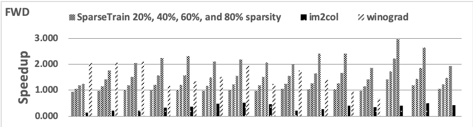
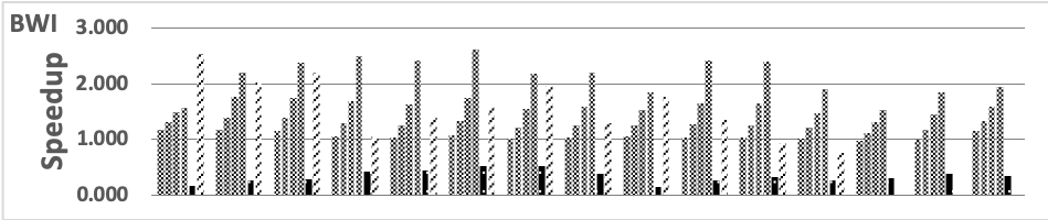
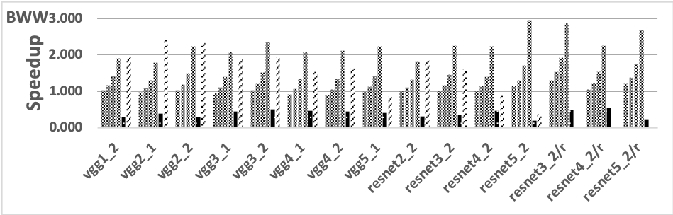
Figure 1. The speedup over direct on the 3x3 layers

$3\times{}3$ ($R=S=3$) has become the most popular convolutional layer type in recent years, so the performance of them is crucial. Techniques such as the Winograd algorithm (Lavin and Gray, [n. d.]) have been proposed to accelerate $3\times{}3$ Layers, and MKL-DNN implements a highly optimized vectorized Winograd convolution that often outperforms direct. However, because the Winograd algorithm reduces computation by transforming the problem to the “Winograd space,” it has two drawbacks that are absent in SparseTrain. First, the transformation introduces numerical instability as the filter size increases, so its application is usually limited to $3\times{}3$ Layers (Vincent et al., 2017); second, it requires additional workspace memory. Further, MKL-DNN’s Winograd implementation does not support strided convolution.

Besides the aforementioned algorithms, MKL-DNN also implements a im2col based convolution. The algorithm flattens and duplicates parts of the input image and the filters to form matrices and then performs matrix multiplication with gemm calls. The version of MKL-DNN that we use incorporates MKL 2019.0 as the backend gemm. Although gemm itself is highly optimized, creating the matrices incurs time and memory overheads, so this implementation is generally slower than direct. Figure 1 shows the speedup of SparseTrain at 20-80% sparsity over direct for all three training components of studied layers. We compare against im2col and Winograd when applicable. Table 4 lists the geo-mean speedup at various sparsity.

At $0\%$ sparsity (i.e., a truly dense input), SparseTrain reaches $92\%$-$95\%$ of direct’s performance on average, depending on the component. This indicates that the overhead to check for and exploit sparsity is low, and the loop order as well as the tiling strategy of SparseTrain are effective.

Table 4. Average speedup at different sparsity for $3\times{}3$ layers

	SparseTrain										im2c.	win.
	$0\%$	$10\%$	$20\%$	$30\%$	$40\%$	$50\%$	$60\%$	$70\%$	$80\%$	$90\%$
FWD	0.92	0.96	1.04	1.13	1.24	1.38	1.56	1.79	2.11	2.48	0.33	1.45
BWI	0.93	0.98	1.06	1.15	1.26	1.40	1.58	1.81	2.10	2.45	0.31	1.48
BWW	0.95	0.98	1.03	1.10	1.18	1.30	1.48	1.76	2.23	3.15	0.37	1.44

On average, the sparsity cross-over point for SparseTrain to outperform direct is between $10\%$-$20\%$, which is lower than the realistic sparsity during training. At $50\%$ sparsity, which is the expected value at the beginning of the training when the distribution of the weights is centered at 0, SparseTrain on average delivers a 1.30x-1.40x speedup.

Typically, the later layers in a network have higher sparsity than the earlier layers. The sparsity reaches over $90\%$ for VGG16 and ResNet-34 layers, and over $80\%$ for ResNet-50 layers. At such level, SparseTrain is on average over 2x faster than direct. On the contrary, im2col is always significantly slower than the baseline. When the stride is 1, Winograd is on average 1.44x-1.48x faster than direct.

SparseTrain performs better at later layers while Winograd dominates at earlier layers. This is partly due to the increased sparsity at later layers; on average, it takes at least $50\%$-$60\%$ sparsity for SparseTrain to surpass Winograd. The other factor is a smaller number of channels for earlier layers, which limits the number of skippable FMAs per input element, and thus reduces efficiency. For example, both vgg1_2 and resnet2_2 have $C$ and $K$ of 64, giving us only 12 skippable FMAs. Since SparseTrain and Winograd have different specialties, they can supplement each other.

With stride 1, SparseTrain for FWD and BWI have similar performance. However, for stride-2 layers (resnet3_2/r, resnet4_2/r, and resnet5_2/r), the former outperforms the latter. As discussed in Section 3.3, $\partial L/\partial D$ needs to be loaded $O^{2}$ times more rapidly during a row sweep in BWI than $Y$ being loaded in FWD. Therefore, BWI suffers from cache bandwidth limitations.

5.2. $1\times{}1$ Convolutional Layers

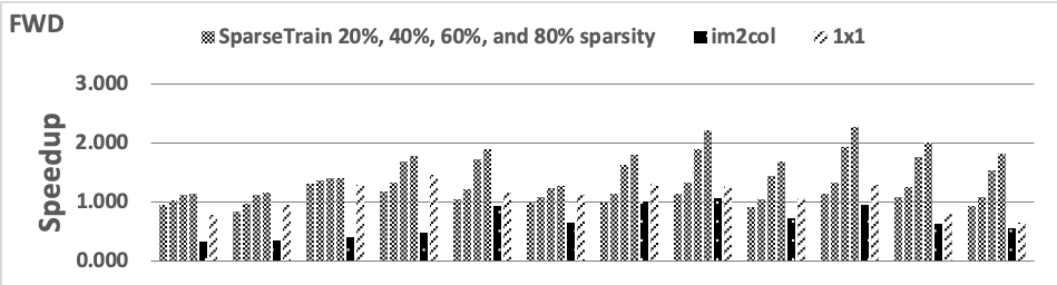
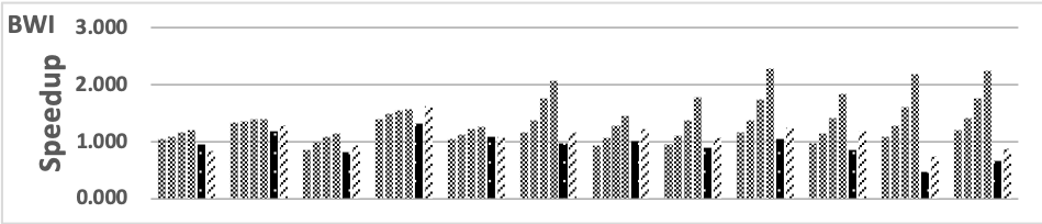
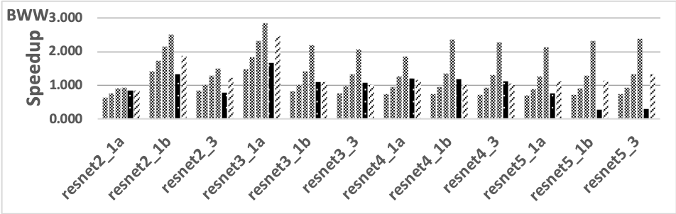
Figure 2. The speedup over direct on the 1x1 layers

$1\times{}1$ layers ($R=S=1$) are widely used in ResNet-50’s bottleneck blocks. They are unique amongst convolutions in that the spatial reuse of $R\times{}S$ is completely absent. As a result, an output element is just a weighted sum of all input channels at the corresponding input $x,y$ location. MKL-DNN provides a specialized algorithm that uses a reduction instead of the accumulation employed by the baseline to specifically deal with $1\times{}1$ Layers. We call it the 1x1 kernel.

Figure 2 shows the speedup on each $1\times{}1$ layer over the dense direct from SparseTrain, im2col, and 1x1. Table 5 lists the average speedup at different sparsity. SparseTrain is developed under the premise that convolution has a high compute-to-memory ratio. However, the ratio for $1\times{}1$ layers is 9x lower than that for $3\times{}3$ layers with the same input/output/channel sizes; thus, as we eliminate useless FMAs, $1\times{}1$ layers may become bandwidth-bound sooner than $3\times{}3$ layers. Therefore, at high sparsity, SparseTrain is less effective on $1\times{}1$ layers than on $3\times{}3$ layers, only reaching 1.66x-2.04x speedup on average at $80\%$ sparsity.

Table 5. Average speedup at different sparsity for $1\times{}1$ layers

	SparseTrain										im2c.	1x1
	$0\%$	$10\%$	$20\%$	$30\%$	$40\%$	$50\%$	$60\%$	$70\%$	$80\%$	$90\%$
FWD	0.97	0.98	1.03	1.09	1.17	1.27	1.39	1.51	1.66	1.78	0.62	1.06
BWI	1.03	1.03	1.08	1.15	1.22	1.33	1.43	1.53	1.66	1.76	0.91	1.08
BWW	0.71	0.76	0.83	0.92	1.05	1.20	1.39	1.66	2.04	2.61	0.87	1.23

We also notice that BWW behaves differently than the other two components. At $0\%$ sparsity, SparseTrain’s performance is on par with the baseline for FWD and BWI. For BWW, though, SparseTrain only reaches $71\%$ of baseline. However, at high sparsity, SparseTrain’s speedup is higher for BWW than the other two components.

Here we compare BWW with FWD. Its difference with BWI can be derived. The difference stems from two competing factors both related to how BWW accesses $\partial L/\partial Y$ against how FWD accesses $Y$. First, BWW uses a different loop order, and in a row sweep touches $V$ times more elements from $\partial L/\partial Y$ than FWD touches $Y$ at $0\%$ sparsity. Second, BWW reads $\partial L/\partial Y$ elements as a memory operand of an FMA. When we skip a group of FMAs, we also skip the access to the $\partial L/\partial Y$ elements. At high sparsity, we eliminate many such access. In contrast, FWD loads and stores $Y$ elements using the cyclic register allocation scheme described in Section 3.2.3, so the $Y$ elements are loaded and stored regardless of sparsity pattern. Therefore, at low sparsity, BWW performs many more memory accesses, and at high sparsity, performs many fewer. The effect of the above factors is less visible at $3\times{}3$ layers thanks to their higher compute-to-memory ratio; however, it surfaces at $1\times{}1$ layers.

The lower channel sizes at earlier $1\times{}1$ layers hurts SparseTrain more than they do at earlier $3\times{}3$ layers due to the absence of spatial reuse. For example, resnet2_1a has 64 for $C$ and $K$, resulting in only 4 FMAs being skippable per zero-checking. Consequently, we can hardly see speedup from SparseTrain on earlier $1\times{}1$ layers. Nonetheless, we can still efficiently leverage the dynamic sparsity in later $1\times{}1$ layers.

On average, the cross-point sparsity for SparseTrain to surpass the specialized 1x1 kernel is below $30\%$ for FWD as well as BWI, and around $50\%$ for BWW.

In addition to $1\times{}1$ and $3\times{}3$ layers, we also experimented with several $5\times{}5$ layers and got even higher speedup. We omit the results due to lack of popularity of the $5\times{}5$ layers.

5.3. Performance at Profiled Sparsity

Rhu et al. (Rhu et al., 2018) observed that during training, the sparsity from ReLU often begins at $\sim$50% but increases rapidly in the first several epoches, and then slowly decreases. Also, later conv layers generally have higher sparsity then earlier layers. They further demonstrated that most of VGG16’s layers are over 80% sparse on average, and some layers’ outputs may reach $90\%$ sparsity on average.

Figure 3 presents the sparsity of each ReLU’s output during our training of the three ResNet Variants. The average sparsity of each layer typically ranges from 20% to 90%, and the observations from Rhu et al. generally hold. One exception is that the degree of sparsity between adjacent layers fluctuates periodically; this is caused by the shortcut in each residual block, which adds positive bias to the outputs of a block and lowers the sparsity from the subsequent ReLU. The fluctuation is more pronounced in ResNet-34 and Fixup ResNet-50 than in ResNet-50.

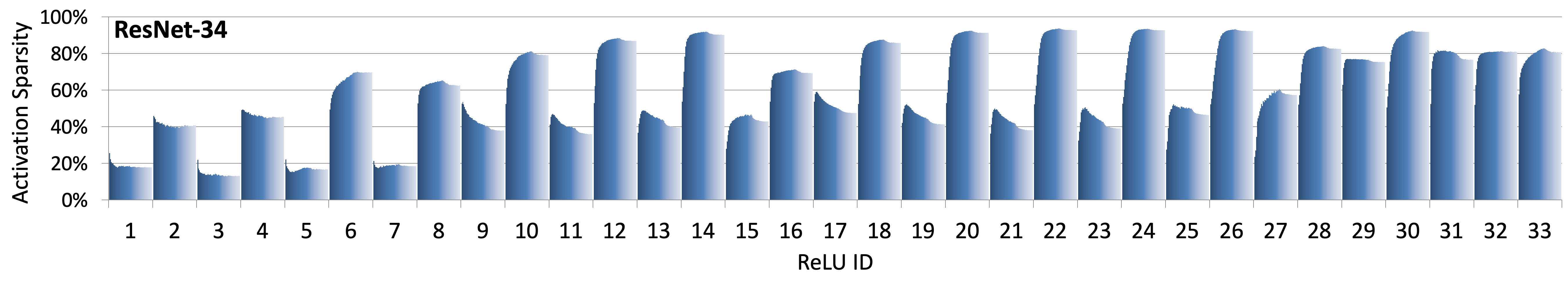
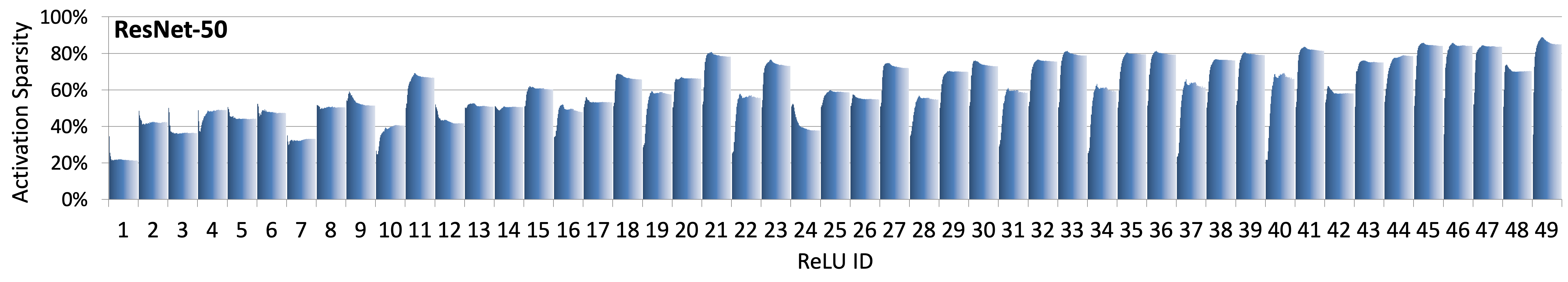
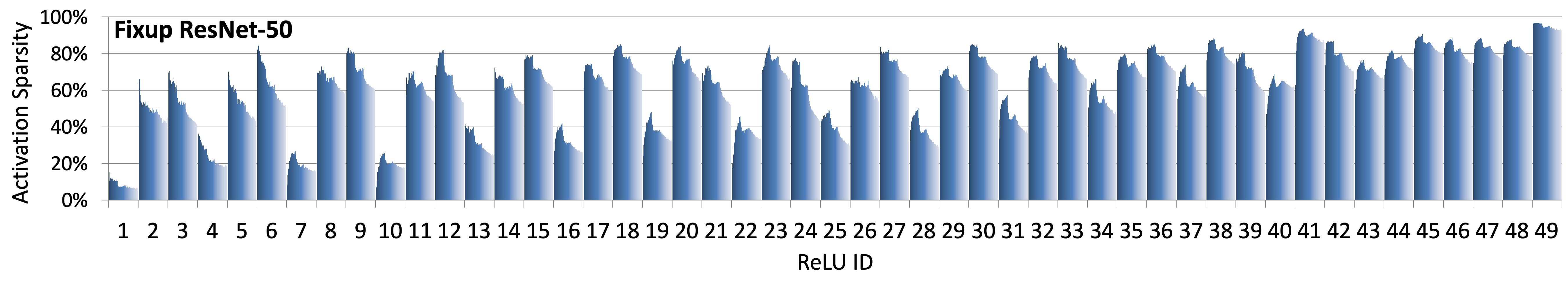
Figure 3. Measured sparsity in ReLU outputs during 100-epoch trainings on ImageNet. Each segment of the x-axis corresponds to a single layer. Within a segment, from left to right are the sparsity from the first epoch to the last.

The inclusion of BatchNorm affects SparseTrain’s execution time of both BWI and BWW. Because ResNet-34/50 has BatchNorm, $\partial L/\partial Y$ has no sparsity, so we replace SparseTrain with the baseline for BWI, and use the sparsity pattern in $D$ to measure the execution time of BWW. On the other hand, VGG-16 and Fixup ResNet-50 do not have BatchNorm, so we use the sparsity pattern in $\partial L/\partial Y$ to measure the execution time of BWI, and choose the higher average sparsity from $D$ or $\partial L/\partial Y$ to measure the execution time of BWW.

Figure 4 illustrates the estimated total execution time of the conv layers with different algorithms during end-to-end training, normalized to the execution time of direct. The plot stacks the execution time of each component. Because SparseTrain is not applicable to the first layers in the network due to the input images often being zero-free, we show the execution time of the first layer as a constant overhead.

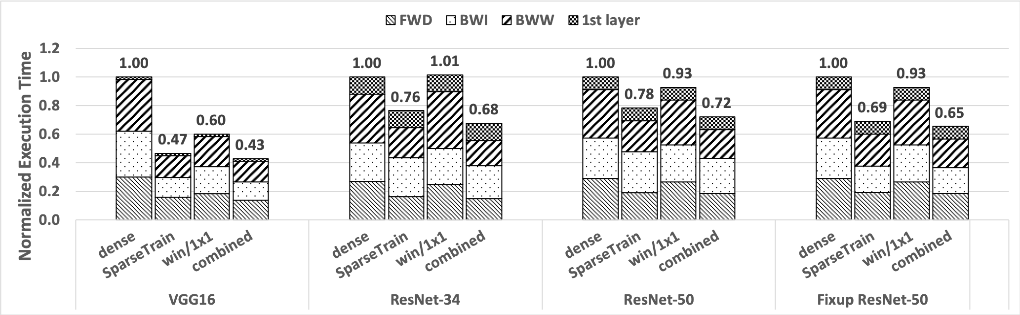
Figure 4. Breakdown of the estimated execution time of all conv layers from networks during end-to-end training, normalized to direct

In the plot, the SparseTrain bars are the execution times of using purely SparseTrain, or in the case of the ResNet-34/50, SparseTrain for FWD and BWW plus the baseline for BWI. The win/1x1 bars are the execution times of using the Winograd convolution or the 1x1 kernel whenever possible. Because we found that SparseTrain and Winograd may complement each other, we also include the combined bars that contain the execution times with the preferred convolution implementation of each layer being employed. Because the im2col implementation is much slower than dense direct, we omit it in the plot.

Table 6 lists the speedup on the conv layers both including and excluding the first layer. The results suggest that when including the first layer, SparseTrain speeds up the training of the conv layers in the studied networks by 1.28x-2.15x. By choosing the best algorithm for each layer, we can speed up training by 1.39x-2.35x. Note that combined chooses the algorithm for each layer statically according to the average execution time. If we profile the sparsity of each layer at intervals during training and then dynamically select the best implementation to use based on the current sparsity level, the potential speedup may be higher.

Table 6. Projected speedup on all conv layers from networks

	Incl. 1st layer			excl. 1st layer
	SparseTrain	win/1x1	comb.	SparseTrain	win/1x1	comb.
VGG16	2.15	1.66	2.35	2.19	1.68	2.40
ResNet-34	1.31	0.99	1.48	1.37	0.98	1.58
ResNet-50	1.28	1.08	1.39	1.31	1.09	1.44
Fixup ResNet-50	1.45	1.08	1.53	1.51	1.09	1.62

SparseTrain can speedup Fixup ResNet-50 by 1.45x instead of 1.28x on the original ResNet-50 thanks to the absence of BatchNorm. We also experimented with minibatch $N=\{32,64\}$, and confirmed that SparseTrain’s execution time scales linearly with $N$.

5.4. Limitations

Apart from the complications caused by BatchNorm, several other factors may limit the application and/or performance of SparseTrain. First, SparseTrain is inapplicable to networks that use activation functions other than ReLU. Nonetheless, ReLU is by far the most popular activation function for CNN.

Second, although we applied Algorithm 3 to combat branch misprediction, the misprediction rate is still noticeable due to the low trip count of the transformed loop ($\leq{}V$). Further reducing mispredictions in software may be hard; however, because the trip count is generated outside of the loop body, previous hardware proposals (Sheikh et al., 2015) can remove the branch misprediction entirely by decoupling trip count generation and loop execution.

Third, the sparsity in FWD and BWI is fully exploited because only one of the two source operands in their FMAs contains sparsity. However, both FMA operands in BWW may be sparse, so the sparsity in BWW is not fully leveraged. Also, SparseTrain does not take advantage of the sparsity in the weights if they are iteratively pruned during training.

Finally, due to the vectorization of the zero-checking in BWW being along the minibatch dimension, we require the batch size to be a multiple of $V$ for maximum performance.

6. Related Works

Various works compress DNN models by eliminating redundant weights. Network pruning  (Han et al., [n. d.]b) (Park et al., 2016) removes redundant network connections under reasonable criteria. Weight quantization (Zhou et al., [n. d.])(Zhu et al., [n. d.]) sacrifices numerical precision to reduce model size. Wen et al. (Wen et al., 2016) studies structured sparsity. Their compressed models are more hardware-friendly. However, they are not applicable during training and do not exploit dynamic sparsity in the activation.

meProp (Sun et al., 2017) sparsifies the back propagation of LSTMs and MLPs by only propagating a small number of gradients in each pass. This reduces back propagation time for the studied networks and lowers overfitting as a byproduct. Yet, it does not affect the forward propagation, nor has it been tested on CNNs. Our work is orthogonal to it and can potentially be applied in conjunction with it.

Several hardware proposals targeting DNN accelerators exploit the sparsity in weights, activations, or both. Cnvlutin (Albericio et al., [n. d.]) leverages sparsity in activations to skip ineffectual computations. Eyeriss (Chen et al., [n. d.]) clock-gates computation path and local buffer when zero is detected in the activation, and it performs convolution in a synchronous manner, collecting partial results from neighbor processing elements, therefore saving energy. However, cycles are not saved. Cambricon-X (Zhang et al., [n. d.]) focuses on weights sparsity and skips multiplications associated with zero weights obtained by pruning. EIE (Han et al., [n. d.]a) exploits the sparsity in both weights and activations using a compressed representation, but it is limited to matrix-vector multiplication (e.g. fully connected layers) and cannot accelerate the most time-consuming convolutional layers. SCNN (Parashar et al., [n. d.]) utilizes the sparsity in both weights and activations, and accelerates the convolution layer. These accelerators modifies the hardware structure while our work is software only.

Normally, the Winograd algorithm (Lavin and Gray, [n. d.]) erase the dynamic sparsity in the activation. Liu et al. (Liu et al., 2017) restore the activation sparsity by applying ReLU to the activation after transforming to the Winograd space. However, their approach changes the network structure. In addition, their focus is to reduce the operation count for running DNN inference on mobile devices, and they do not target training nor efficient vectorized implementation.

7. Conclusion

The widespread usage of the ReLU non-linear activation function in DNNs means that DNN training includes a significant fraction of computations on zero values. Traditional sparse methods, however, are not effective since the fraction of zeros is modest, and the locations of zeros are dynamic.

We observe that each output value from a ReLU function sees significant reuse in all three phases of training. Therefore, if we order the main compute loops appropriately, we can check for zero on the fly, and potentially jump over chunks of work. We further vectorize the sparsity-checking, maximize efficiency when sparsity levels are low, and minimize branch mispredictions. When applied to direct convolutions, at $0\%$ sparsity, our approach generally performs within $10\%$ of a highly optimized dense code. For training of real DNNs, our approach is projected to outperform the dense convolutions by 1.31x-2.19x.

This paper is the first work to exploit dynamic sparsity with only software techniques and opens up new research direction in speeding up computation with modest sparsity.

References

- [1]
- ama [[n. d.]] [n. d.]. Amazon SageMaker ML Instance Types. https://aws.amazon.com/sagemaker/pricing/instance-types/.
- fro [[n. d.]] [n. d.]. Frontera System - Texas Advanced Computing Center. https://www.tacc.utexas.edu/systems/frontera.
- nvi [[n. d.]] [n. d.]. GPU-Based Deep Learning Inference: A Performance and Power Analysis. https://www.nvidia.com/content/tegra/embedded-systems/pdf/jetson_tx1_whitepaper.pdf.
- mkl [[n. d.]] [n. d.]. Intel(R) Math Kernel Library for Deep Neural Networks (Intel(R) MKL-DNN). https://github.com/intel/mkl-dnn.
- lei [[n. d.]] [n. d.]. SuperMUC-NG - Leibniz-Rechenzentrum (LRZ) Dokumentation. https://doku.lrz.de/display/PUBLIC/SuperMUC-NG.
- xby [[n. d.]] [n. d.]. Xbyak: JIT assembler for x86(IA32), x64(AMD64, x86-64) by C++. https://github.com/herumi/xbyak.
- Albericio et al. [[n. d.]] Jorge Albericio, Patrick Judd, Tayler Hetherington, Tor Aamodt, Natalie Enright Jerger, and Andreas Moshovos. [n. d.]. Cnvlutin: Ineffectual-neuron-free Deep Neural Network Computing (ISCA’16).
- Amodei et al. [2015] Dario Amodei, Rishita Anubhai, Eric Battenberg, Carl Case, Jared Casper, Bryan Catanzaro, Jingdong Chen, Mike Chrzanowski, Adam Coates, Greg Diamos, Erich Elsen, Jesse Engel, Linxi Fan, Christopher Fougner, Tony Han, Awni Hannun, Billy Jun, Patrick LeGresley, Libby Lin, Sharan Narang, Andrew Ng, Sherjil Ozair, Ryan Prenger, Jonathan Raiman, Sanjeev Satheesh, David Seetapun, Shubho Sengupta, Yi Wang, Zhiqian Wang, Chong Wang, Bo Xiao, Dani Yogatama, Jun Zhan, and Zhenyao Zhu. 2015. Deep Speech 2: End-to-End Speech Recognition in English and Mandarin. arXiv:cs.CL/1512.02595
- C. Wu [[n. d.]] K. Chen D. Chen S. Choudhury M. Dukhan K. Hazelwood E. Isaac Y. Jia B. Jia T. Leyvand H. Lu Y. Lu V. Peter B. Reagen F. Sun A. Tulloch X. Wang Y. Wang B. Wasti R. Xian S. Yoo P. Zhang C. Wu, D. Brooks. [n. d.]. Machine Learning at Facebook: Understanding Inference at the Edge. In HPCA’19.
- Chen et al. [[n. d.]] Yu-Hsin Chen, Joel Emer, and Vivienne Sze. [n. d.]. Eyeriss: A Spatial Architecture for Energy-efficient Dataflow for Convolutional Neural Networks (ISCA’16).
- Georganas et al. [2018] Evangelos Georganas, Sasikanth Avancha, Kunal Banerjee, Dhiraj Kalamkar, Greg Henry, Hans Pabst, and Alexander Heinecke. 2018. Anatomy of high-performance deep learning convolutions on simd architectures. In SC18: International Conference for High Performance Computing, Networking, Storage and Analysis. IEEE, 830–841.
- Gitman and Ginsburg [2017] Igor Gitman and Boris Ginsburg. 2017. Comparison of batch normalization and weight normalization algorithms for the large-scale image classification. arXiv preprint arXiv:1709.08145 (2017).
- Han et al. [[n. d.]a] Song Han, Xingyu Liu, Huizi Mao, Jing Pu, Ardavan Pedram, Mark A. Horowitz, and William J. Dally. [n. d.]a. EIE: Efficient Inference Engine on Compressed Deep Neural Network (ISCA’16).
- Han et al. [[n. d.]b] Song Han, Huizi Mao, and William J. Dally. [n. d.]b. Deep Compression: Compressing Deep Neural Network with Pruning, Trained Quantization and Huffman Coding (ICLR’16).
- Han et al. [[n. d.]c] Song Han, Jeff Pool, John Tran, and William J. Dally. [n. d.]c. Learning both Weights and Connections for Efficient Neural Networks (NIPS’15).
- Hazelwood et al. [[n. d.]] Kim Hazelwood, Sarah Bird, David Brooks, Soumith Chintala, Utku Diril, Dmytro Dzhulgakov, Mohamed Fawzy, Bill Jia, Yangqing Jia, Aditya Kalro, James Law, Kevin Lee, Jason Lu, Pieter Noordhuis, Misha Smelyanskiy, Liang Xiong, and Xiaodong Wang. [n. d.]. Applied Machine Learning at Facebook: A Datacenter Infrastructure Perspective. In HPCA’18.
- He et al. [[n. d.]] Kaiming He, Xiangyu Zhang, Shaoqing Ren, and Jian Sun. [n. d.]. Deep Residual Learning for Image Recognition (CVPR’16).
- Howard et al. [2017] Andrew G. Howard, Menglong Zhu, Bo Chen, Dmitry Kalenichenko, Weijun Wang, Tobias Weyand, Marco Andreetto, and Hartwig Adam. 2017. MobileNets: Efficient Convolutional Neural Networks for Mobile Vision Applications. CoRR abs/1704.04861 (2017). arXiv:1704.04861 http://arxiv.org/abs/1704.04861
- Huang et al. [2017] Gao Huang, Zhuang Liu, Laurens van der Maaten, and Kilian Q. Weinberger. 2017. Densely Connected Convolutional Networks. 2017 IEEE Conference on Computer Vision and Pattern Recognition (CVPR) (2017), 2261–2269.
- Ioffe and Szegedy [2015] Sergey Ioffe and Christian Szegedy. 2015. Batch normalization: Accelerating deep network training by reducing internal covariate shift. arXiv preprint arXiv:1502.03167 (2015).
- Ji et al. [2018] H. Ji, L. Song, L. Jiang, H. H. Li, and Y. Chen. 2018. ReCom: An efficient resistive accelerator for compressed deep neural networks. In 2018 Design, Automation Test in Europe Conference Exhibition (DATE). https://doi.org/10.23919/DATE.2018.8342009
- Jouppi et al. [[n. d.]] Norman P. Jouppi, Cliff Young, Nishant Patil, David Patterson, Gaurav Agrawal, Raminder Bajwa, Sarah Bates, Suresh Bhatia, Nan Boden, Al Borchers, Rick Boyle, Pierre-luc Cantin, Clifford Chao, Chris Clark, Jeremy Coriell, Mike Daley, Matt Dau, Jeffrey Dean, Ben Gelb, Tara Vazir Ghaemmaghami, Rajendra Gottipati, William Gulland, Robert Hagmann, Richard C. Ho, Doug Hogberg, John Hu, Robert Hundt, Dan Hurt, Julian Ibarz, Aaron Jaffey, Alek Jaworski, Alexander Kaplan, Harshit Khaitan, Andy Koch, Naveen Kumar, Steve Lacy, James Laudon, James Law, Diemthu Le, Chris Leary, Zhuyuan Liu, Kyle Lucke, Alan Lundin, Gordon MacKean, Adriana Maggiore, Maire Mahony, Kieran Miller, Rahul Nagarajan, Ravi Narayanaswami, Ray Ni, Kathy Nix, Thomas Norrie, Mark Omernick, Narayana Penukonda, Andy Phelps, Jonathan Ross, Amir Salek, Emad Samadiani, Chris Severn, Gregory Sizikov, Matthew Snelham, Jed Souter, Dan Steinberg, Andy Swing, Mercedes Tan, Gregory Thorson, Bo Tian, Horia Toma, Erick Tuttle, Vijay Vasudevan, Richard Walter, Walter Wang, Eric Wilcox, and Doe Hyun Yoon. [n. d.]. In-Datacenter Performance Analysis of a Tensor Processing Unit (ISCA’17).
- Krizhevsky et al. [[n. d.]] Alex Krizhevsky, Ilya Sutskever, and Geoffrey E. Hinton. [n. d.]. Imagenet classification with deep convolutional neural networks. In Advances in Neural Information Processing Systems (NIPS’12).
- Lavin and Gray [[n. d.]] Andrew Lavin and Scott Gray. [n. d.]. Fast Algorithms for Convolutional Neural Networks (CVPR’16).
- Liu et al. [2017] Xingyu Liu, Jeff Pool, Song Han, and William J. Dally. 2017. Efficient Sparse-Winograd Convolutional Neural Networks. CoRR abs/1802.06367 (2017).
- Maas et al. [[n. d.]] Andrew L Maas, Awni Y Hannun, and Andrew Y Ng. [n. d.]. Rectifier nonlinearities improve neural network acoustic models (ICML’13).
- Parashar et al. [[n. d.]] Angshuman Parashar, Minsoo Rhu, Anurag Mukkara, Antonio Puglielli, Rangharajan Venkatesan, Brucek Khailany, Joel Emer, Stephen W. Keckler, and William J. Dally. [n. d.]. SCNN: An Accelerator for Compressed-sparse Convolutional Neural Networks (ISCA’17).
- Park et al. [2016] Jongsoo Park, Sheng Li, Wei Wen, Ping Tak Peter Tang, Hai Li, Yiran Chen, and Pradeep Dubey. 2016. Faster CNNs with Direct Sparse Convolutions and Guided Pruning (ICLR’16).
- Radford et al. [2015] Alec Radford, Luke Metz, and Soumith Chintala. 2015. Unsupervised representation learning with deep convolutional generative adversarial networks. arXiv preprint arXiv:1511.06434 (2015).
- Rhu et al. [2018] Minsoo Rhu, Mike O’Connor, Niladrish Chatterjee, Jeff Pool, Youngeun Kwon, and Stephen W Keckler. 2018. Compressing DMA engine: Leveraging activation sparsity for training deep neural networks. In 2018 IEEE International Symposium on High Performance Computer Architecture (HPCA). IEEE, 78–91.
- Sen et al. [2017] Sanchari Sen, Shubham Jain, Swagath Venkataramani, and Anand Raghunathan. 2017. SparCE: Sparsity aware General Purpose Core Extensions to Accelerate Deep Neural Networks. arXiv:cs.DC/1711.06315
- Sheikh et al. [2015] Rami Sheikh, James Tuck, and Eric Rotenberg. 2015. Control-flow decoupling: An approach for timely, non-speculative branching. IEEE Trans. Comput. 64, 8 (2015), 2182–2203.
- Silver et al. [2016] David Silver, Aja Huang, Chris J. Maddison, Arthur Guez, Laurent Sifre, George van den Driessche, Julian Schrittwieser, Ioannis Antonoglou, Veda Panneershelvam, Marc Lanctot, Sander Dieleman, Dominik Grewe, John Nham, Nal Kalchbrenner, Ilya Sutskever, Timothy Lillicrap, Madeleine Leach, Koray Kavukcuoglu, Thore Graepel, and Demis Hassabis. 2016. Mastering the Game of Go with Deep Neural Networks and Tree Search. Nature 529, 7587 (Jan. 2016), 484–489. https://doi.org/10.1038/nature16961
- Simonyan and Zisserman [[n. d.]] Karen Simonyan and Andrew Zisserman. [n. d.]. Very deep convolutional networks for large-scale image recognition. ArXiv’14 ([n. d.]).
- Simonyan and Zisserman [2014] Karen Simonyan and Andrew Zisserman. 2014. Very Deep Convolutional Networks for Large-Scale Image Recognition. CoRR abs/1409.1556 (2014). http://arxiv.org/abs/1409.1556
- Sun et al. [2017] Xu Sun, Xuancheng Ren, Shuming Ma, and Houfeng Wang. 2017. meProp: Sparsified Back Propagation for Accelerated Deep Learning with Reduced Overfitting. In Proceedings of the 34th International Conference on Machine Learning (Proceedings of Machine Learning Research), Vol. 70. International Convention Centre, Sydney, Australia, 3299–3308.
- Szegedy et al. [[n. d.]] Christian Szegedy, Wei Liu, Yangqing Jia, Pierre Sermanet, Scott Reed, Dragomir Anguelov, Dumitru Erhan, Vincent Vanhoucke, and Andrew Rabinovich. [n. d.]. Going Deeper with Convolutions (CVPR’15). http://arxiv.org/abs/1409.4842
- Takahashi [2018] Dean Takahashi. 2018. Gadi Singer interview - How Intel designs processors in the AI era. https://venturebeat.com/2018/09/09/gadi-singer-interview-how-intel-designs-processors-in-the-ai-era/
- Vincent et al. [2017] Kevin Vincent, Kevin Stephano, Michael Frumkin, Boris Ginsburg, and Julien Demouth. 2017. On improving the numerical stability of winograd convolutions. (2017).
- Wen et al. [2016] Wei Wen, Chunpeng Wu, Yandan Wang, Yiran Chen, and Hai Li. 2016. Learning Structured Sparsity in Deep Neural Networks. CoRR abs/1608.03665 (2016). arXiv:1608.03665 http://arxiv.org/abs/1608.03665
- Yu et al. [[n. d.]] Jiecao Yu, Andrew Lukefahr, David Palframan, Ganesh Dasika, Reetuparna Das, and Scott Mahlke. [n. d.]. Scalpel: Customizing DNN Pruning to the Underlying Hardware Parallelism. In ISCA’17.
- Zhang et al. [2019] Hongyi Zhang, Yann N Dauphin, and Tengyu Ma. 2019. Fixup Initialization: Residual Learning Without Normalization. arXiv preprint arXiv:1901.09321 (2019).
- Zhang et al. [[n. d.]] S. Zhang, Z. Du, L. Zhang, H. Lan, S. Liu, L. Li, Q. Guo, T. Chen, and Y. Chen. [n. d.]. Cambricon-X: An accelerator for sparse neural networks (MICRO’16).
- Zhou et al. [[n. d.]] Aojun Zhou, Anbang Yao, Yiwen Guo, Lin Xu, and Yurong Chen. [n. d.]. Incremental Network Quantization: Towards Lossless CNNs with Low-Precision Weights (ICLR’17).
- Zhu et al. [[n. d.]] Chenzhuo Zhu, Song Han, Huizi Mao, and William J Dally. [n. d.]. Trained ternary quantization (ICLR’17).