HILUCSI: Simple, Robust, and Fast Multilevel ILU
for Large-Scale Saddle-Point Problems from PDEs

Abstract

Incomplete factorization is a widely used preconditioning technique for Krylov subspace methods for solving large-scale sparse linear systems. Its multilevel variants, such as ILUPACK, are more robust for many symmetric or unsymmetric linear systems than the traditional, single-level incomplete LU (or ILU) techniques. However, the previous multilevel ILU techniques still lacked robustness and efficiency for some large-scale saddle-point problems, which often arise from systems of partial differential equations (PDEs). We introduce HILUCSI, or Hierarchical Incomplete LU-Crout with Scalability-oriented and Inverse-based dropping. As a multilevel preconditioner, HILUCSI statically and dynamically permutes individual rows and columns to the next level for deferred factorization. Unlike ILUPACK, HILUCSI applies symmetric preprocessing techniques at the top levels but always uses unsymmetric preprocessing and unsymmetric factorization at the coarser levels. The deferring combined with mixed preprocessing enabled a unified treatment for nearly or partially symmetric systems and simplified the implementation by avoiding mixed $1\times 1$ and $2\times 2$ pivots for symmetric indefinite systems. We show that this combination improves robustness for indefinite systems without compromising efficiency. Furthermore, to enable superior efficiency for large-scale systems with millions or more unknowns, HILUCSI introduces a scalability-oriented dropping in conjunction with a variant of inverse-based dropping. We demonstrate the effectiveness of HILUCSI for dozens of benchmark problems, including those from the mixed formulation of the Poisson equation, Stokes equations, and Navier-Stokes equations. We also compare its performance with ILUPACK and the supernodal ILUTP in SuperLU.

1 Introduction

Krylov subspace (KSP) methods, such as GMRES [1, 2] and BiCGSTAB [3], are widely used for solving large-scale sparse unsymmetric or indefinite linear systems, especially those arising from numerical discretizations of partial differential equations (PDEs). For relatively ill-conditioned matrices, the KSP methods can significantly benefit from a robust and efficient preconditioner. Among these preconditioners, incomplete LU (or ILU) is one of the most successful. Given a linear system $\boldsymbol{A}\boldsymbol{x}=\boldsymbol{b}$, the ILU, or more precisely incomplete LDU (or ILDU) factorization of $\boldsymbol{A}$ is an approximate factorization

$$\boldsymbol{P}^{T}\boldsymbol{A}\boldsymbol{Q}\approx\boldsymbol{L}\boldsymbol{D}\boldsymbol{U}.$$ (1)

On the right-hand side, $\boldsymbol{D}$ is a diagonal matrix, $\boldsymbol{L}$ is a unit lower triangular matrix, and $\boldsymbol{U}$ is an upper triangular matrix; on the left-hand side, $\boldsymbol{P}$ and $\boldsymbol{Q}$ are row and column permutation matrices, respectively. Let $\boldsymbol{M}=\boldsymbol{L}\boldsymbol{D}\boldsymbol{U}$, and $\boldsymbol{P}\boldsymbol{M}\boldsymbol{Q}^{T}$ is then a preconditioner of $\boldsymbol{A}$, or equivalently $\boldsymbol{M}$ is a preconditioner of $\boldsymbol{P}^{T}\boldsymbol{A}\boldsymbol{Q}$. We consider only right preconditioning in this work. Given the ILU factorization, a right-preconditioned KSP method solves the preconditioned linear system

$$\boldsymbol{A}\left(\boldsymbol{P}\boldsymbol{M}\boldsymbol{Q}^{T}\right)^{-1}\boldsymbol{y}=\boldsymbol{b},$$ (2)

which ideally would converge much faster than solving the original linear system, and then $\boldsymbol{x}=\left(\boldsymbol{P}\boldsymbol{M}\boldsymbol{Q}^{T}\right)^{-1}\boldsymbol{y}=\boldsymbol{Q}\boldsymbol{U}^{-1}\boldsymbol{D}^{-1}\boldsymbol{L}^{-1}\boldsymbol{P}^{T}\boldsymbol{y}$.

Earlier ILU methods, such as ILUTP [4, 1], lack robustness for some indefinite systems (see, e.g., [5, 6, 7]). More recently, multilevel ILU (MLILU) techniques [8, 9, 10], a.k.a. multilevel block factorization [11], have significantly improved the robustness of ILU for many applications. A two-level preconditioner $\hat{\boldsymbol{M}}$ for the permuted matrix $\boldsymbol{P}^{T}\boldsymbol{A}\boldsymbol{Q}$ can be constructed via the approximation

$$\boldsymbol{P}^{T}\boldsymbol{A}\boldsymbol{Q}=\begin{bmatrix}\hat{\boldsymbol{B}}&\hat{\boldsymbol{F}}\\ \hat{\boldsymbol{E}}&\hat{\boldsymbol{C}}\end{bmatrix}\approx\hat{\boldsymbol{M}}=\begin{bmatrix}\tilde{\boldsymbol{B}}&\tilde{\boldsymbol{F}}\\ \tilde{\boldsymbol{E}}&\hat{\boldsymbol{C}}\end{bmatrix}=\begin{bmatrix}\boldsymbol{L}_{B}&\boldsymbol{0}\\ \boldsymbol{L}_{E}&\boldsymbol{I}\end{bmatrix}\begin{bmatrix}\boldsymbol{D}_{B}&\boldsymbol{0}\\ \boldsymbol{0}&\boldsymbol{S}_{C}\end{bmatrix}\begin{bmatrix}\boldsymbol{U}_{B}&\boldsymbol{U}_{F}\\ \boldsymbol{0}&\boldsymbol{I}\end{bmatrix},$$ (3)

where $\hat{\boldsymbol{B}}\approx\tilde{\boldsymbol{B}}=\boldsymbol{L}_{B}\boldsymbol{D}_{B}\boldsymbol{U}_{B}$, $\hat{\boldsymbol{E}}\approx\tilde{\boldsymbol{E}}=\boldsymbol{L}_{E}\boldsymbol{D}_{B}\boldsymbol{U}_{B}$, and $\hat{\boldsymbol{F}}\approx\tilde{\boldsymbol{F}}=\boldsymbol{L}_{B}\boldsymbol{D}_{B}\boldsymbol{U}_{F}$. The permutation matrices $\boldsymbol{P}$ and $\boldsymbol{Q}$ may be obtained from some static reordering, static or dynamic pivoting, or a combination of them. The Schur complement, i.e.,

$$\boldsymbol{S}_{C}=\hat{\boldsymbol{C}}-\tilde{\boldsymbol{E}}\tilde{\boldsymbol{B}}^{-1}\tilde{\boldsymbol{F}}=\hat{\boldsymbol{C}}-\boldsymbol{L}_{E}\boldsymbol{D}_{B}\boldsymbol{U}_{F},$$ (4)

is further approximately factorized recursively, resulting in a multilevel ILU. In [12], ILUPACK [13, 8], which is a state-of-the-art MLILU package, was shown to be significantly more robust than ILUTP and algebraic multigrid preconditioners [14] for indefinite systems. Nevertheless, the robustness and efficiency of MLILU remained a challenge for saddle-point systems with millions or more unknowns, which often arise from discretizations of Stokes, Navier-Stokes, and Helmholtz equations, in computational fluid dynamics, climate modeling, multiphysics coupling, etc.

The objective of this work is to improve the robustness and efficiency of MLILU for saddle-point systems from PDEs. Our preconditioner was motivated by two key observations. First, we observe that many linear systems from systems of PDEs are “nearly” or “partially” symmetric, with some block structures. Without loss of generality, assume matrix $\boldsymbol{A}\in\mathbb{R}^{n\times n}$ has the form

$$\boldsymbol{A}=\begin{bmatrix}\boldsymbol{B}&\boldsymbol{F}\\ \boldsymbol{E}&\boldsymbol{C}\end{bmatrix}.$$ (5)

It is worth noting that $\hat{\boldsymbol{B}}$ in (3) may have different sizes from $\boldsymbol{B}$ in (5) due to permutation. For linear systems from PDEs, the nonzero pattern of $\boldsymbol{A}$ is often nearly symmetric, because in some commonly used numerical methods (such as finite differences [15], finite elements [16, 17], or finite volumes [18]), the local support of the basis functions (a.k.a. trial functions in finite elements) and that of the test functions in the variational formulations are often the same or have significant overlap. In addition, the numerical values are often nearly symmetric (i.e., $\left\|\boldsymbol{A}-\boldsymbol{A}^{T}\right\|\ll\left\|\boldsymbol{A}\right\|$), because the numerical asymmetry is often due to small non-self-adjoint terms (such as advection in a diffusion-dominant advection-diffusion problem [17, p. 243]) or due to truncation errors (such as in a Petrov-Galerkin method for a self-adjoint PDE [17, p. 88]). For systems of PDEs, $\boldsymbol{A}$ may be partially symmetric in that $\left\|\boldsymbol{B}-\boldsymbol{B}^{T}\right\|\ll\left\|\boldsymbol{B}\right\|$ for the reasons mentioned above, but $\boldsymbol{E}$ and $\boldsymbol{F}^{T}$ differ significantly. Such partial symmetry may be due to strongly imposed constraints in a variational formulation [19], high-order treatment of Neumann boundary conditions in finite elements [20] or finite differences [15], imposition of jump conditions in immersed/embedded boundary methods [21, 22], etc. Second, we observe that the state-of-the-art direct solvers, such as MUMPS [23] and PARDISO [24], are highly optimized in terms of cache performance, but they tend to scale superlinearly as the problem sizes increase. In contrast, MLILU has poor locality due to the dynamic nature of droppings, but its multilevel structure offers additional opportunities to achieve near-linear time complexity while being as robust as possible for very large systems, such as those with millions or more unknowns.

Based on the preceding observations, we introduce a new preconditioner, called HILUCSI (pronounced as Hi-Luxi), which stands for Hierarchical Incomplete LU-Crout with Scalability-oriented and Inverse-based dropping. As the name suggests, HILUCSI is a multilevel-ILU preconditioner that utilizes the Crout version of ILU [25]. In this aspect, HILUCSI is closely related to ILUPACK [13]. The inverse-based dropping [26, 27, 8] in HILUCSI is also based on that of ILUPACK. However, HILUCSI improves robustness and efficiency through a novel combination of several techniques. First, HILUCSI is designed to take advantage of the near or partial symmetry of the linear systems in a multilevel fashion. Specifically, we apply symmetric preprocessing at the top levels for nearly or partially symmetric matrices and apply unsymmetric factorization at lower levels for all indefinite systems. This combination differs from other earlier techniques for taking advantage of partial symmetry, such as using $(\boldsymbol{A}+\boldsymbol{A}^{T})/2$ as an algebraic preconditioner of $\boldsymbol{A}$ [28, 29] or using the self-adjoint parts of the differential operators as a physics-based preconditioner [30].

Second, to construct its multilevel structure, HILUCSI introduces a static deferring strategy to avoid nearly zero diagonal entries, in conjunction with dynamic deferring for avoiding uncontrolled growth of the condition numbers of $\boldsymbol{L}_{B}$ and $\boldsymbol{U}_{B}$ in (3) at each level. Here, deferring refers to a symmetric permutation operation that delays some rows and their corresponding columns at one level to the next level for deferred factorization. The dynamic deferring in HILUCSI is similar to that in ILUPACK. Due to deferring, $\hat{\boldsymbol{B}}$ is in general smaller than $\boldsymbol{B}$ in HILUCSI. This behavior makes HILUCSI different from, and potentially more robust than, a straightforward block preconditioner for partially symmetric matrices where $\hat{\boldsymbol{B}}$ is a simple permutation of $\boldsymbol{B}$ [31]. In addition, the static deferring in HILUCSI simplifies its implementation for (nearly) symmetric saddle-point problems, by eliminating the need of Bunch-Kaufman pivoting [32, 33] as in [34, 35] or similar $2\times 2$ block permutations as described in [36].

Third, to achieve efficiency for large-scale problems, HILUCSI introduces a scalability-oriented dropping, which we use in conjunction with inverse-based dropping. The primary goal of our scalability-oriented dropping is to achieve (near) linear-time complexity in the number of nonzeros in the input matrix. Although this goal shares some similarity to the space-based droppings (such as those in ILUT [37], ICMF [38], PARDISO [24]) as well as area-based dropping in [6], it is different in that linear-time complexity implies linear-space complexity but not vice versa. We show that the scalability-oriented dropping along with mixed symmetric and unsymmetric preprocessing enabled HILUCSI to deliver superior robustness and efficiency compared to the previous state of the art, such as ILUPACK [13] and supernodal ILUTP [6], for saddle-point problems from PDEs.

The remainder of the paper is organized as follows. In Section 2, we review some background on incomplete LU factorization and its multilevel variants. In Section 3, we describe the algorithm components of HILUCSI. Section 4 presents numerical results with HILUCSI as a right preconditioner for restarted GMRES and compares its performance with some state-of-the-art packages. Finally, Section 5 concludes the paper with a discussion on future work. For completeness, we present some analyses of stability and efficiency in the appendix.

2 Preliminaries and related work

In this section, we review some incomplete LU preconditioners. Because there is a vast literature on preconditioning and ILU, we review only some of the most relevant techniques and their mathematical analysis. For comprehensive reviews, we refer readers to some surveys [39, 40, 41, 42] and textbooks [1, 43].

2.1 Single-level ILU

The basic form of ILU in (1), which we refer to as the single-level ILU (versus multilevel ILU), has been used to solve linear systems from PDEs since the 1950s [44]. In 1977, Meijerink and van der Vorst [45] showed that incomplete Cholesky (IC) factorization is stable for a symmetric M-matrix, i.e., a matrix with nonpositive off-diagonal entries and nonnegative entries in its inverse. Since then, IC has been extended to and become popular for SPD systems [46, 47, 38, 48]. However, ILU for unsymmetric or indefinite systems is significantly more challenging, and it has been an active research topic over the past few decades; see, e.g., [4, 6, 37, 49, 50].

2.1.1 Variants of single-level ILU.

In its simplest form, ILU does not involve any pivoting, and $\boldsymbol{L}$ and $\boldsymbol{U}$ preserve the sparsity patterns of the lower and upper triangular parts of $\boldsymbol{P}^{T}\boldsymbol{A}\boldsymbol{Q}$, respectively. This approach is often referred to as ILU0 or ILU(0). To improve its robustness, one may allow fills, a.k.a. fill-ins, which are new nonzeros in the $\boldsymbol{L}$ and $\boldsymbol{U}$ factors. The fills may be introduced based on their levels in the elimination tree or based on the magnitude of numerical values. The former leads to the so-called ILU($k$), which zeros out all the fills of level $k+1$ or higher in the elimination tree. The combination of the two is known as ILU with dual thresholding (ILUT) [37]. The level-based fills may be replaced with some other dropping to control the numbers of fills in each row or column. The ILU algorithms in PETSc [51] and hypre [14] use some variants of ILUT.

ILUT may encounter zero or tiny pivots, which can lead to a breakdown of the factorization. One may replace tiny pivots with a small value, but such a trick is not robust [4]. The robustness may be improved by using pivoting, leading to the so-called ILUP [52] and ILUTP [1]. The ILU implementations in MATLAB [53], SPARSKIT [54], and the supernodal ILU in SuperLU [6], for example, are based on ILUTP. However, ILUTP cannot prevent small pivots [10], so it is still not robust in practice; see, e.g., [6, 56, 10] and Section 4 in this work for some failed cases with ILUTP.

Another single-level ILU technique is the Crout-version of ILU, a.k.a. ILUC [25, 35]. In the context of symmetric matrices, ILUC is also known as the left-looking ILU [57]. At the $k$th step, ILUC updates of the $k$th column in $\boldsymbol{L}$, which we denote by $\boldsymbol{\ell}_{k}$, using the previous $k-1$ columns in $\boldsymbol{L}$, and it updates the $k$th row of $\boldsymbol{U}$, which denoted by $\boldsymbol{u}_{k}^{T}$ , in a similar fashion. Unlike the standard $ijk$-ordered or “right-looking” ILU, ILUC updates $\boldsymbol{\ell}_{k}$ and $\boldsymbol{u}_{k}^{T}$ as late as possible. As a result, it allows dropping nonzeros in $\boldsymbol{\ell}_{k}$ and $\boldsymbol{u}_{k}^{T}$ as late as possible and avoids premature dropping or partially updated columns. HILUCSI uses ILUC within each level, along with some static and dynamic deferring described in Section 3.2.

2.1.2 Accuracy and stability of single-level preconditioner.

For the ILU to be a “robust” preconditioner, it should be accurate and stable. For the sake of simplicity, let us omit the permutation matrices $\boldsymbol{P}$ and $\boldsymbol{Q}$ in the discussions, and assume $\boldsymbol{M}=\boldsymbol{L}\boldsymbol{D}\boldsymbol{U}$ in (1) is the preconditioner of $\boldsymbol{A}$. Following [39], we measure the accuracy and stability of $\boldsymbol{M}$ by $\left\|\boldsymbol{A}-\boldsymbol{M}\right\|$ and $\left\|\boldsymbol{A}\boldsymbol{M}^{-1}-\boldsymbol{I}\right\|$, respectively. In [39], the Frobenius norm was used for its ease of computation. We may use any other norm for the convenience of analysis.

The accuracy of the preconditioner mostly depends on the dropping strategies: Without dropping, $\left\|\boldsymbol{A}-\boldsymbol{M}\right\|$ is expected to be accurate up to machine precision. Most ILU techniques utilize some form of dual thresholding [37], by combining a numerical-value-based dropping and a combinatorial-structure-based dropping. Several numerical-value-based dropping strategies have been proposed for single-level ILU; see, e.g., [26] and [50]. These dropping strategies are often used with a space-based dropping. To reduce space-based dropping, some fill-reduction permutation, such as reverse Cuthill-Mckee (RCM) [58] and approximate minimum degree (AMD) [59], are sometimes performed. In terms of stability, for $\left\|\boldsymbol{A}\boldsymbol{M}^{-1}-\boldsymbol{I}\right\|$ to be small (or bounded), $\|\boldsymbol{L}^{-1}\|$ and $\|\boldsymbol{U}^{-1}\|$ must be bounded by some small constant, as pointed out by Bollhöfer [26]. In addition, a tiny diagonal value in $\boldsymbol{D}$ would also cause $\left\|\boldsymbol{A}\boldsymbol{M}^{-1}-\boldsymbol{I}\right\|$ to blow up, which corresponds to the danger of tiny pivots in ILU, as emphasized by Chow and Saad in [4]. To improve the accuracy of ILU for some elliptic PDEs, Dupont et al. [60] introduced modified ILU (MILU). MILU modifies the diagonal entries to compensate for the discarded entries so that the sum of each row is preserved. This technique appears to be quite popular; see, e.g., [61, 62, 6]. However, we do not use MILU, because it was ineffective for linear systems from more general PDEs in our testing.

The dual requirements of accuracy and stability cause a dilemma for single-level ILU for large-scale systems from PDEs, because the condition number of $\boldsymbol{A}$, $\kappa(\boldsymbol{A})$, grows as the number of unknowns $n$ increases. Specifically, it is well known that for parabolic or elliptic PDEs, $\kappa(\boldsymbol{A})$ is inversely proportional to $h^{-2}$ for some edge length measure $h$ [15, 17]. Assuming isotropic meshes, we expect $\kappa(\boldsymbol{A})$ to be proportional to $\mathcal{O}(n^{2/d})$, where $d$ is the topological dimension of the domain. Assuming $\boldsymbol{A}$ is normalized such that $\|\boldsymbol{A}\|=\Theta(1)$, so is $\|\boldsymbol{M}\|$. If $\boldsymbol{M}$ contains the physically meaningful “modes” of the PDE that correspond to the smallest singular values of $\boldsymbol{A}$, then $\left\|\boldsymbol{M}^{-1}\right\|\approx\|\boldsymbol{A}^{-1}\|$, and $\left\|\boldsymbol{U}^{-1}\right\|\left\|\boldsymbol{D}^{-1}\right\|\left\|\boldsymbol{L}^{-1}\right\|\geq\left\|\boldsymbol{M}^{-1}\right\|\approx\mathcal{O}(n^{2/d})$. Hence, it is challenging, if not impossible, to devise accurate single-level ILU that is also stable (i.e., with bounded $\left\|\boldsymbol{L}^{-1}\right\|$, $\left\|\boldsymbol{D}^{-1}\right\|$, and $\left\|\boldsymbol{U}^{-1}\right\|$) for large-scale systems from PDEs. Note that although some preprocessing techniques (such as equilibration [63, 64]) can be applied to reduce $\|\boldsymbol{A}^{-1}\|$ and $\left\|\boldsymbol{M}^{-1}\right\|$, but they cannot alter this asymptotic behavior.

2.2 Multilevel ILU

2.2.1 Variants of MLILU.

The aforementioned difficulties of single-level ILU are mitigated by leveraging the multilevel structure in an MLILU. There are numerous variants of MLILU in the literature, such as those in ILUM [65], BILUTM [66], ARMS [67], ILUPACK [13, 8], MDRILU [68], ILU++ [69, 56], etc. Among these, ILUPACK, MDRILU, and ILU++ aim to improve the robustness (and potentially also the efficiency) of ILU using dynamic permutations. HILUCSI shares similar goals as these preconditioners. Some methods use static reordering to improve robustness in ILUT within a block, such as [70, 71], which we do not consider due to their lack of dynamic control of the stability of triangular factors. Note that some MLILU techniques, such as those in ILUM and BILUTM, were developed to expose parallelism, and some others, such as those in [72, 9, 73], constructed an algebraic analogy of multigrid methods. The parallelization of ILU and the mathematical connection between MLILU and multigrid methods are beyond the scope of this work.

2.2.2 Accuracy and stability of MLILU preconditioner.

Let us assume $\hat{\boldsymbol{M}}$ in (3) is a preconditioner of $\boldsymbol{P}^{T}\boldsymbol{A}\boldsymbol{Q}$. We need to compute $\hat{\boldsymbol{M}}^{-1}\boldsymbol{u}$ for a block vector $\boldsymbol{u}=\begin{bmatrix}\boldsymbol{u}_{1}\\ \boldsymbol{u}_{2}\end{bmatrix}$, i.e.,

$$\hat{\boldsymbol{M}}^{-1}\boldsymbol{u}=\begin{bmatrix}\tilde{\boldsymbol{B}}^{-1}\boldsymbol{u}_{1}\\ \boldsymbol{0}\end{bmatrix}+\begin{bmatrix}-\tilde{\boldsymbol{B}}^{-1}\hat{\boldsymbol{F}}\\ \boldsymbol{I}\end{bmatrix}\boldsymbol{S}_{C}^{-1}(\boldsymbol{u}_{2}-\hat{\boldsymbol{E}}\tilde{\boldsymbol{B}}^{-1}\boldsymbol{u}_{1}),$$ (6)

where $\boldsymbol{u}_{1}$ and $\boldsymbol{u}_{2}$ corresponds to $\hat{\boldsymbol{B}}$ and $\hat{\boldsymbol{C}}$, respectively. The stable computation of $\hat{\boldsymbol{M}}^{-1}\boldsymbol{u}$ requires the stable computation of $\tilde{\boldsymbol{B}}^{-1}\boldsymbol{u}_{1}$, which in turn requires $\left\|\boldsymbol{L}_{B}^{-1}\right\|$, $\left\|\boldsymbol{D}_{B}^{-1}\right\|$, and $\left\|\boldsymbol{U}_{B}^{-1}\right\|$ to be bounded by a constant at each level, analogous to the boundedness of $\left\|\hat{\boldsymbol{B}}\tilde{\boldsymbol{B}}^{-1}-\boldsymbol{I}\right\|$ for single-level ILU. Unlike single-level ILU, MLILU can permute rows and columns (such as permuting those in $\boldsymbol{B}$ that lead to large condition numbers of $\boldsymbol{L}_{B}$ and $\boldsymbol{U}_{B}$ to the trailing block $\hat{\boldsymbol{C}}$) for deferred factorization, as proposed in ILUPACK [13, 8]. HILUCSI takes a similar approach to ensure the well-conditioning of $\tilde{\boldsymbol{B}}$, except that it uses different permutation strategies than that of ILUPACK for (nearly) symmetric indefinite systems.

For the preconditioner $\hat{\boldsymbol{M}}$ to be stable, it is clear that the computation of $\boldsymbol{S}_{C}^{-1}\boldsymbol{u}_{2}$ (or $\boldsymbol{S}_{C}^{-1}\boldsymbol{v}$ for $\boldsymbol{v}=\boldsymbol{u}_{2}-\hat{\boldsymbol{E}}\tilde{\boldsymbol{B}}^{-1}\boldsymbol{u}_{1}$) should also be as stable as possible. To this end, we apply the MLILU on $\boldsymbol{S}_{C}$ recursively until $\boldsymbol{S}_{C}$ is small enough for a dense factorization. As in single-level ILU, the stability of the computation can be improved by performing equilibration [63, 64] before applying MLILU on $\boldsymbol{S}_{C}$. Although these preprocessing strategies are used in virtually all the MLILU techniques, HILUCSI differs from them in its combination of symmetric preprocessing at the top levels with unsymmetric preprocessing at the coarse levels.

In terms of the accuracy of MLILU, the concerns within each level are similar to those of single-level ILU, as described in Section 2.1.2. For example, the dropping strategies in ILUPACK [8] and ILU++ [69, 56] are variants of their single-level ILU in [26] and [50], respectively. The accuracy of the Schur complement in (4) is an additional concern in MLILU. In [8], Bollhöfer and Saad proposed to improve the accuracy by using a formulation due to Tismenetsky [74], which, unfortunately, often leads to excessive fills. A simpler alternative is to tighten the dropping criteria for the Schur complement, as used in [13, 56, 67, 68]. In this work, we use the latter strategy.

2.3 Near-linear time preconditioners

In this work, we aim at devising an accurate and stable preconditioner that has near-linear time complexity. In particular, the preconditioner $\hat{\boldsymbol{M}}$ should be constructed in (near) linear time in the number of nonzeros in the input matrix $\boldsymbol{A}$, and $\boldsymbol{M}^{-1}\boldsymbol{u}$ can be computed in (near) linear time for any $\boldsymbol{u}\in\mathbb{R}^{n}$. Note that ILU0 or ILUTP with some space-based dropping may have linear space complexity, but they may still have superlinear time complexity. Our objective near-linear time complexity is similar to that of Hackbusch’s hierarchical matrices [75]. However, Hackbusch measures the accuracy by some norm of $\boldsymbol{A}-\boldsymbol{M}$, without taking into account the stability condition on $\boldsymbol{A}\boldsymbol{M}^{-1}-\boldsymbol{I}$ for preconditioners [39]. For linear systems arising from finite difference or finite element discretizations for PDEs, the number of nonzeros per row is typically bounded by a constant. For such systems, our objective is to achieve near-linear time complexity in the number of unknowns, similar to algebraic multigrid methods for elliptic PDEs [76]. This objective is also similar to that of AMLI for SPD systems [77]. However, we aim to solve unsymmetric and indefinite systems, for which the state-of-the-art multigrid methods (such as BoomerAMG in hypre [14]) are not robust [12], and AMLI is inapplicable.

3 Hierarchical ILU with scalability-oriented droppings

In this section, we describe the overall algorithm of HILUCSI. As an MLILU, HILUCSI shares a similar control flow and some components as others, such as ILUPACK and ILU++, except that we adapt the dropping strategies to achieve better scalability for large-scale systems, we adapt the pivoting/deferring strategies for simplicity for indefinite systems without compromising robustness, and we adapt the preprocessing, thresholds, and factorization techniques at different levels to take into account near or partial symmetry of the systems. Figure 1 gives a schematic of the factorization procedure in HILUCSI, which takes a sparse matrix $\boldsymbol{A}$, some thresholds for dropping and permutations, along with a flag indicating near-symmetry as input. In a nutshell, the algorithm dynamically builds a hierarchy of levels by using static and dynamic deferring. Depending on whether the leading block in the present level is symmetric or nearly symmetric, it performs symmetric or unsymmetric preprocessing and factorization correspondingly, and it performs a complete dense factorization at the coarsest level. The algorithm returns the $\boldsymbol{L}_{B}$, $\boldsymbol{D}_{B}$, $\boldsymbol{U}_{B}$, $\tilde{\boldsymbol{E}}$, and $\tilde{\boldsymbol{F}}$ of each level, which can then be used to compute (6). In the following, we focus on three key components of HILUCSI: the scalability-oriented dropping with each level, the deferring strategies for constructing the next level, and the mixed preprocessing strategies for taking advantage of near and partial symmetry.

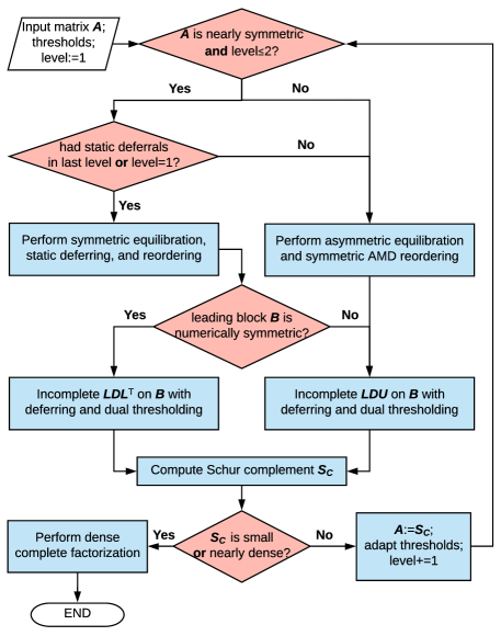
Figure 1: Flowchart of the multilevel ILDU factorization in HILUCSI.

3.1 Scalability-oriented dropping

We first describe the core component of HILUCSI in the computation at each level. For simplicity, let us omit the permutations (i.e., deferring) for now so that we can focus on the dropping strategy in a two-level ILU by assuming $\boldsymbol{B}=\hat{\boldsymbol{B}}$. Since one of the main objectives of HILUCSI is to achieve efficiency for large-scale systems, we introduce a scalability-oriented dropping specifically designed for MLILU. This dropping strategy has two parts. First, we limit the number of nonzeros (nnz) in the $k$th column of $\boldsymbol{L}$, namely $\boldsymbol{\ell}_{k}$, by a factor of the nnz in the corresponding column in the input matrix, i.e.,

$$\text{nnz}(\boldsymbol{\ell}_{k})\leq\alpha\max\{\text{nnz}(\boldsymbol{a}_{k}),0.85\,\overline{\text{nnz}}(\boldsymbol{a}_{*})\},$$ (7)

where $\alpha$ is a user-controllable parameter, and we refer to it as the nnz factor. The term $\overline{\text{nnz}}(\boldsymbol{a}_{*})$ denotes the average number of nonzeros in the columns of the input matrix $\boldsymbol{A}$, and it is introduced to prevent excessive dropping for columns with very few nonzeros in a highly nonuniform matrix. Similarly, we limit the nnz in the rows of $\boldsymbol{U}$ in a similar fashion. Second, when computing the Schur complement using (4), we apply dropping to limit the nnz in each column in $\boldsymbol{U}_{F}$ based on the right-hand side of (7), and similarly for each row in $\boldsymbol{L}_{E}$.

Remark 1.

The two parts of the scalability-oriented dropping help control the time complexity of updating $\boldsymbol{L}$ and $\boldsymbol{U}$ and computing the Schur complement, respectively. The first part is easily incorporated into the Crout version of ILU. In particular, at the $k$th step, after updating $\boldsymbol{\ell}_{k}$ (and $\boldsymbol{u}_{k}^{T}$), we only keep up to $m$ largest-magnitude nonzeros, where $m$ is equal to the right-hand side of (7). The second part controls the time complexity of the sparse matrix-matrix multiplication. It is important to note that in a multilevel setting, $\text{nnz}(\boldsymbol{a}_{k})$ in (7) is the number of nonzeros in the $k$th column of the input matrix $\boldsymbol{A}$ (assuming no permutation), instead of that of the Schur complement from the previous level. For completeness, in Appendix B we present additional implementation details and a more detailed argument of the linear time complexity of these two core steps within each level.

Besides the scalability-oriented dropping, HILUCSI also employs a numerical-value-based strategy as a secondary dropping. We adopted the inverse-based dropping as proposed in [26] and [8]. More specifically, we estimate $\tilde{\kappa}_{L,k}\approx\left\|\boldsymbol{L}_{k}^{-1}\right\|_{\infty}$ and $\tilde{\kappa}_{U,k}\approx\left\|\boldsymbol{U}_{k}^{-1}\right\|_{1}$ incrementally as described in [78]. Given a user-tunable threshold $\kappa_{D}$ on $\left\|\boldsymbol{D}_{B}^{-1}\right\|_{\infty}$ for the level, we drop the $i$th nonzero in $\boldsymbol{\ell}_{k}$ if

$$\kappa_{D}\tilde{\kappa}_{L,k}|\ell_{ik}|\leq\tau,$$ (8)

and we drop the $j$th nonzero in $\boldsymbol{u}_{k}^{T}$ if

$$\kappa_{D}\tilde{\kappa}_{U,k}|u_{kj}|\leq\tau.$$ (9)

We refer to $\tau$ as the drop tolerance (or in short, droptol). Like $\alpha$, $\tau$ is also a user-controllable threshold, and it may vary from level to level. This inverse-based dropping can be readily incorporated into the Crout version of ILU [25].

Remark 2.

The inverse-based dropping described above was first proposed for single-level ILU by Bollhöfer [26]. It was later adopted by Li et al. in Crout version of ILU [25] and then further adapted to multilevel ILU by Bollhöfer and Saad in [8]. Note that in [8], Bollhöfer and Saad replaced $\tilde{\kappa}_{L,k}$ and $\tilde{\kappa}_{U,k}$ with a user-specified parameter $\kappa$, which is an upper-bound of $\tilde{\kappa}_{L,k}$ and $\tilde{\kappa}_{U,k}$. Hence, our inverse-based dropping is closer to its original form in [26] than that in [8]. However, the scaling factor $\kappa_{D}$ in (8) and (9) was not present in [26]. Although $\kappa_{D}$ may be blended into $\tau$, we find it conceptually clearer to separate out $\kappa_{D}$, since $\kappa_{D}$ arises from the stability analysis of the leading block as we summarize in Appendix A. $\kappa_{D}$ is also relevant in the deferring strategy for building the multilevel structure, as we discuss next.

3.2 Static and dynamic permutations for deferred factorization

The discussions in Section 3.1 omitted permutations. It is well known that without permutations, small pivots can make Gaussian elimination unstable [33], and similar for ILU [4]. However, pivoting (such as partial pivoting in ILUTP [52, 1], row pivoting in the supernodal ILUTP [6], and dual pivoting in ILU++ [79]) requires sophisticated data structures to implement. For symmetric indefinite systems, the Bunch-Kaufman pivoting [32, 33] (such as in [35] and in [36]) incurs additional implementation complexities by requiring permuting a combination of $1\times 1$ and $2\times 2$ pivots.

In HILUCSI, we exploit the multilevel structure to simplify both the data structure and algorithm by only permuting the rows and the corresponding columns in the leading block to the trailing blocks and deferring them to the next level. We refer to this permutation strategy as deferring. In particular, we utilize two types of deferring. First, at the $k$th step of Crout update, we dynamically permute the row and column to the lower-right corner if the diagonal is smaller than a threshold ($\kappa_{D}$) or one of the estimated norms $\left\|\boldsymbol{L}_{B}^{-1}\right\|_{\infty}$ and $\left\|\boldsymbol{U}_{B}^{-1}\right\|_{1}$ exceeds some threshold ($\kappa_{L}$ and $\kappa_{U}$). We refer to this as dynamic deferring, which is effective in resolving zero or tiny pivots in most cases. In addition, we defer the zero and tiny diagonal entries a priori. We refer to this as static pivoting. In our experiments, we found that static pivoting is advantageous, especially for saddle-point problems that have many zero diagonal entries, probably because zero or tiny pivots tend to lead to rapid growth of $\left\|\boldsymbol{L}_{B}^{-1}\right\|_{\infty}$ and $\left\|\boldsymbol{U}_{B}^{-1}\right\|_{1}$.

The static and dynamic deferring strategies in HILUCSI naturally result in a multilevel structure, where within each level, we apply the algorithm described in Section 3.1. To implement HILUCSI efficiently, we need a data structure that supports efficient sequential access of the $k$th row of $\boldsymbol{L}$ along with all the rows in $\boldsymbol{U}_{1:k-1,k:n}$, and similarly for the corresponding column in $\boldsymbol{U}$ and $\boldsymbol{L}_{k:n,1:k-1}$, as required by the $k$th step of the Crout ILU. To this end, we use a bi-index data structure based on that proposed by Li, Saad, and Chow for the Crout version of ILU without pivoting for unsymmetric matrices [25], which was based on that proposed by Jones and Plassmann [47] for the row-version of incomplete Cholesky factorization. The original data structures in [25] and [47] did not support pivoting, but they require only about half of the storage and less data movement than the more sophisticated data structures for ILU with pivoting in [35] and [56]. Since HILUCSI utilizes only static and dynamic deferring, we can extend the more efficient data structure in [4, 25] to support deferring without the extra memory overhead in [35] and [56]. In particular, we allow the indices to have a gap equal to the number of deferred rows and columns within each level, and we eliminate the gap at the end of the ILU factorization in the current level.

In terms of the thresholds, we use the same $\kappa_{D}$ for dynamic deferring as that in (8) and (9) for inverse-based dropping. It typically suffices for $\kappa_{L}=\kappa_{U}=\kappa_{D}$, so we can simply use $\kappa$ to denote their threshold and refer to it as condest. In terms of the thresholds, we observe from numerical experimentation that it is desirable to tighten the thresholds in level two by doubling $\alpha$, reducing $\tau$ by a factor of 10, and reducing $\kappa$ by a factor of two while restricting $\kappa\geq 2$. From level three, we revert $\alpha$ to the original value for efficiency, while preserving the refined $\tau$ and $\kappa$. This choice is because the dropping in $\boldsymbol{S}_{C}$ is amplified by $\tilde{\boldsymbol{B}}^{-1}$ in the term $-\tilde{\boldsymbol{B}}^{-1}\hat{\boldsymbol{F}}\boldsymbol{S}_{C}^{-1}\hat{\boldsymbol{E}}\tilde{\boldsymbol{B}}^{-1}$ in (6), and the accuracy and stability of level two appear to be the most important because it is the largest Schur complement.

Remark 3.

The dynamic deferring described above is similar to that for unsymmetric matrices in [8]. In [36], Schenk et al. described a dynamic deferring strategy for symmetric indefinite systems, which permuted a combination of $1\times 1$ and $2\times 2$ blocks, motivated by the Bunch-Kaufman pivoting. The static deferring in HILUCSI appears to be new. It eliminates the need of pivoting or deferring of $2\times 2$ blocks, and in turn, significantly simplifies the treatment for symmetric indefinite systems without compromising robustness or efficiency.

It is worth noting that deferring is not foolproof. For example, if the thresholds are too tight, then many rows and columns may be deferred, leading to too many levels, undermining the robustness and also the goal of near-linear time complexity. As another example, a matrix may have all zero diagonals in the extreme case, and static deferring would defer the whole matrix to the next level indefinitely. We mitigate this issue by resorting to unsymmetric preprocessing and unsymmetric factorization in coarse levels, as we address next.

3.3 Mixed symmetric and unsymmetric factorization and preprocessing

In HILUCSI, a novel feature is that it mixes symmetric and unsymmetric techniques at different levels, to improve robustness and efficiency for nearly or partially symmetric matrices. This mixed procedure has two aspects. First, for matrices that are symmetric or partially symmetric, i.e., the leading block $\boldsymbol{B}$ is symmetric in the input, but $\boldsymbol{E}$ may or may not be equal to $\boldsymbol{F}^{T}$, we apply symmetric factorization to $\boldsymbol{B}$, with static and dynamic deferring. This combination allows HILUCSI to save the factorization time by up to 50% at the top levels for partially symmetric matrices. However, we always resort to unsymmetric factorization at the coarser levels. As alluded to in Section 3.2, this mixed factorization allows HILUCSI to avoid indefinite deferring when there are a large number of tiny diagonal entries in the input. In our experiments, the benefits of improving robustness outweigh the potential computational cost, since the coarser levels have small sizes; see Section 4.3 for more detail.

Secondly, HILUCSI employs different preprocessing techniques, including reordering and equilibration, at different levels. As we noted in Section 2.1.2, fill-reduction reordering (such as RCM and AMD) reduces the effect of droppings, and equilibration improves the stability of the factorization by reducing the condition numbers of the triangular factors. For nearly or partially symmetric matrices, we apply reordering and equilibration symmetrically. In particular, we apply RCM on $\text{nzp}(\boldsymbol{A})+\text{nzp}(\boldsymbol{A}^{T})$, where nzp denotes the nonzero pattern. In terms of equilibration, we use MC64 [80, 81] to compute the row permutation vector $\boldsymbol{P}_{r}$ and the row and column scaling vectors $\boldsymbol{D}_{r}$ and $\boldsymbol{D}_{c}$, respectively. To preserve symmetry, we perform a post-processing step by setting $\boldsymbol{P}_{r}=\boldsymbol{P}_{c}$ and $\tilde{\boldsymbol{D}}_{r}=\tilde{\boldsymbol{D}}_{c}=\sqrt{\boldsymbol{D}_{r}\boldsymbol{D}_{c}}$. At coarser levels where we apply unsymmetric factorization, we always use AMD reordering and MC64 equilibration directly. If the matrix is unsymmetric, we apply reordering on $\text{nzp}(\boldsymbol{A})+\text{nzp}(\boldsymbol{A}^{T})$, where denotes the nonzero pattern. In terms of the overall control flow of preprocessing, we apply equilibration first, then static deferring, and finally fill-reduction reordering on the leading block.

Remark 4.

The mixed factorization and preprocessing improve the robustness for nearly and partially symmetric matrices, especially those arising from systems of PDEs, as we will show in Section 4.3. We chose RCM and AMD for symmetric and unsymmetric reordering, respectively, because it has previously been shown that RCM works better than AMD for single-level ILU for symmetric matrices [82, 46]. We also observed similar behavior for multilevel ILU in our experiments, probably because RCM tends to lead to smaller off-diagonal blocks, which tends to improve the quality of the multilevel ILU. In terms of symmetric equilibration, we use our own implementation of MC64 and the symmetrization process similar to that in HSL_MC64 [83]. In [84], Duff and Pralet described a sophisticated algorithm for symmetric indefinite systems, which involves $2\times 2$ pivots and is more difficult to implement.

3.4 Overall time complexity of HILUCSI

In terms of the computational cost, the core components of HILUCSI achieve linear-time complexity at each level in the number of unknowns for sparse linear systems from PDEs; see Appendix B for a detailed analysis. Note HILUCSI uses a complete dense factorization in the last level, which has a cubic time complexity in its number of rows and columns but excellent cache performance. To ensure the overall linear-time complexity of factorization, we terminate the recursion of HILUCSI when the final Schur complement is no more than $\max\left\{n^{1/3},C\right\}$ rows and columns, where $n$ is the size of the original user input and $C$ is a constant. Base on our experimentation, we found that $C=500$ leads to a negligible dense-factorization cost. However, it is worth noting that the preprocessing components in Section 3.3 may have superlinear complexity in the worst case. In particular, AMD has quadratic-time complexity in the worst case [85, 81]. In contrast, RCM has linear-time complexity [58], which is yet another reason for using RCM instead of AMD at the top levels. MC64 is superlinear in the worst case, but fortunately, it has an expected linear-time complexity for most systems from PDEs [81]. Hence, we claim that HILUCSI achieves near-linear time complexity overall at each level. Note that the number of levels in HILUCSI may grow as the problem size increases, albeit very slowly. In Section 4, we will show that HILUCSI indeed scales nearly linearly and performs better than both ILUPACK and SuperLU for large systems with millions of unknowns.

4 Numerical results

We have implemented HILUCSI using the C++-11 standard. In this section, we assess the robustness and efficiency of our implementation for some challenging benchmark problems and compare its performance against some state-of-the-art packages. In particular, we chose ILUPACK v2.4 [13, 86] as the representative of multilevel ILU, partially because HILUCSI is based on the same Crout-version of multilevel ILU as in ILUPACK, and more importantly, ILUPACK has been optimized for both unsymmetric and symmetric matrices. In comparison with other packages, our tests showed that ILUPACK outperformed ARMS in ITSOL v2 [67] by up to an order of magnitude for larger unsymmetric systems. The improvement was even more significant for symmetric systems. In our tests, ILUPACK was also significantly more robust than ILU++ [69, 56]. We chose the supernodal ILUTP in SuperLU v5.2.1 [55, 6] as a representative of the state-of-the-art single-level ILU. In all of our tests, we used right-preconditioning for restarted GMRES, with the dimension of the Krylov subspace limited to 30, i.e., GMRES(30). We used $10^{-6}$ for the relative tolerance of GMRES and limited the number of iterations to $500$. For HILUCSI and ILUPACK, we used our implementation of flexible GMRES [1]; for SuperLU, we used GMRES implemented in PETSc v3.11.3.

We conducted our tests on a single node of a cluster running CentOS 7.4 with two 2.5 GHz 12-core Intel Xeon E5-2680v3 processors and 64 GB of RAM. We compiled HILUCSI, SuperLU, and PETSc all using GCC 4.8.5 with the optimization option -O3, and we used the binary release of ILUPACK v2.4 for GNU64. We accessed ILUPACK through its MATLAB mex functions, of which the overhead is negligible. For accurate timing, both turbo and power-saving modes were turned off for the processors.

4.1 Baseline as “black-box” preconditioners

As a baseline study, we assess HILUCSI for some benchmark problems in the literature. We collected more than 60 larger-scale benchmark problems that were highlighted in some recent ILU publications, which were mostly from the SuiteSparse Matrix Collections [87] and the Matrix Market [88]. For ill-conditioned linear systems, we only consider those with a meaningful right-hand side. We present results on some of the most challenging benchmark problems that were highlighted in [8], [6], and [7], together with two larger unsymmetric systems for Navier-Stokes (N-S) equations. Table 1 summarizes these unsymmetric matrices, including their application areas, types, sizes, and estimated condition numbers. Among the problems omitted here, HILUCSI failed only for the system invextr1_new in [7], which has a large null-space dimension of 2,910 and also caused failures for all the methods tested in [7]. In addition, we generated two sets of symmetric indefinite systems using FEniCS v2017.1.0 [89] by discretizing the 3D Stokes equation and the mixed formulation of the Poisson equation. These equations have a wide range of applications in computational fluid dynamics (CFD), solid mechanics, heat transfer, etc. We discretized the former using Taylor–Hood elements [90] and discretized the latter using a mixture of linear Brezzi-Douglas-Marini (BDM) elements [91] and degree-0 discontinuous Galerkin elements [92]. These problems are challenging because the matrices have some nonuniform block structures, and they have many zeros in the diagonals. To facilitate the scalability study, for each set, we generated three linear systems using meshes of different resolutions. Note that the matrices generated by FEniCS do not enforce symmetry exactly and contain some nearly zero values due to rounding errors. We manually filtered out the small values that are close to machine precision and then enforced symmetry using $(\boldsymbol{A}+\boldsymbol{A}^{T})/2$. For this baseline comparison, we used droptol $\tau=10^{-4}$ for all the codes, as in [6], and used the recommended defaults for the other parameters for most problems. For ILUPACK, we used MC64 matching, AMD ordering, and condest (i.e., $\kappa$) 5. For SuperLU, when using its default options, we could solve four problems. We doubled its “fill factor” from 10 to 20, which allowed SuperLU to solve another five problems. For HILUCSI, we used nnz factor $\alpha=10$ and condest $\kappa=3$ for all the cases.

In Table 1, we report the overall runtimes (including both factorization and solve times), numbers of GMRES iterations, and the nnz ratios (i.e., the ratios of the number of nonzeros in the output versus that in the input matrix, also known as the fill ratio [6]) for each code. The fastest runtime for each case is highlighted in bold. HILUCSI had a 95% success rate for these problems with the default parameters, and it was the fastest for 65% of the cases. For twotone, which is not a PDE-based problem, we could not solve it unless we enlarge $\alpha$ to $15$. We note that for all of the test cases, the final Schur complements in HILUCSI had fewer than 500 rows and columns. ILUPACK solved 80% of cases and it was the fastest for 10% of the cases. Among the failed cases, ILUPACK ran out of the main memory for RM07R. For the symmetric problems, ILUPACK automatically detects symmetric matrices and then applies ILDL^T factorization with mixed $1\times 1$ and $2\times 2$ pivots automatically. This optimization in ILUPACK benefited its timing for those problems but hurt its robustness for the two larger systems from Stokes equations, which we could solve only by explicitly forcing ILUPACK to use unsymmetric ILU. ILUPACK was unable to solve PR02R, regardless of how we tuned its parameters. SuperLU was the least robust among the three: It solved only 45% of cases, and it was the fastest for 25% of cases. Note that for the largest system solved by all the codes, namely atmosmodl, HILUCSI outperformed ILUPACK and SuperLU by a factor of 6 and 9, respectively. On the other hand, for a medium-sized problem, namely e40r5000, SuperLU outperformed HILUCSI and ILUPACK by a factor of 7.5 and 15, respectively. This result shows that supernodal ILUTP excels in cache performance, but its ILUTP is fragile compared to multilevel ILU in ILUPACK and HILUCSI. Overall, HILUCSI delivered the best robustness and efficiency for these cases.

Table 1: Baseline comparison of HILUCSI, ILUPACK, and SuperLU, denoted as H, I, and S, respectively, using robust parameters (droptol $10^{-4}$ for all and $\alpha=10$ for HILUCSI). $\times$, and $-$ indicate failed factorization and stagnation of GMRES(30), respectively. HILUCSI failed for twotone with $\alpha=10$, but it took 7.71 seconds with $\alpha=15$. For SuperLU, ‘*’ indicates doubling fill-factor. The leaders are in bold.

Matrix	Appl.	n	nnz	Cond.	factor. time (sec.)			total time (sec.)			GMRES iter.			nnz ratio
					H	I	S	H	I	S	H	I	S	H	I	S
nearly symmetric, indefinite systems from PDEs
venkat01	2D Euler	62,424	1,717,792	2.5e6	6.70	8.29	5.49	6.81	8.40	5.91	3	3	3	6.3	5.8	8.7
rma10	3D CFD	46,835	2,374,001	4.4e10	10.5	31.6	4.46	10.6	31.7	4.73	2	2	2	5.8	8.7	6.0
mixtank_new		29,957	1,995,041	2.2e11	39.7	128	$-$	40.2	128	$-$	9	3	$-$	15	41	$-$
Goodwin_071	3D	56,021	1,797,934	1.4e7	20.2	15.4	6.45	20.8	15.5	16.3	13	3	81	15	8.2	9.2
Goodwin_095	Navier-	100,037	3,226,066	3.4e7	38.2	42.3	19.8	39.9	42.6	21.1*	18	3	4	16	9.2	12
Goodwin_127	Stokes	178,437	5,778,545	8.2e7	70.9	95.1	62.3	75.1	95.1	65.0*	24	3	4	16	12	15
RM07R	(N-S)	381,689	37,464,962	2.2e11	3.1e3	$\times$	$\times$	3.3e3	$\times$	$\times$	75	$\times$	$\times$	44	$\times$	$\times$
PR02R	2D N-S	161,070	8,185,136	1.1e21	256	$-$	$-$	261	$-$	$-$	14	$-$	$-$	28	$-$	$-$
e40r5000		17,281	553,956	2.5e10	18.0	36.8	2.26	18.7	36.8	2.4*	22	2	3	40	37	11
xenon2	materials	157,464	3,866,688	1.4e5	43.7	198	$-$	44.8	198	$-$	9	3	$-$	14	22	$-$
atmosmodl	Helmholtz	1,489,752	10,319,760	1.5e3	78.2	496	608	85.1	502	718	16	6	125	12	27	8.9
other unsymmetric systems
onetone1	circuit	36,057	335,552	9.4e6	0.39	0.92	$-$	0.44	1.12	$-$	11	5	$-$	3.3	3.0	$-$
twotone	simulation	120,750	1,224,224	4.5e9	$-$	18.3	$-$	$-$	18.5	$-$	$-$	2	$-$	$-$	12	$-$
bbmat	2D airfoil	38,744	1,771,722	5.4e8	31.4	36.4	57.2	31.9	36.5	59.0*	9	3	8	17	13	18
symmetric, saddle-point problems from PDEs
S3D1	3D Stokes	18,037	434,673	1.2e7	1.63	6.40	7.68	1.63	6.56	9.90*	2	1	41	11	53	19
S3D2		121,164	3,821,793	8.9e7	80.3	$\times$	$\times$	80.7	$\times$	$\times$	4	$\times$	$\times$	10	$\times$	$\times$
S3D3		853,376	31,067,368	6.3e8	777	$\times$	$\times$	781	$\times$	$\times$	4	$\times$	$\times$	13	$\times$	$\times$
M3D1	3D	29,404	522,024	1.7e5	6.57	8.28	$-$	6.66	8.31	$-$	5	3	$-$	15	19	$-$
M3D2	mixed	211,948	4,109,496	2.3e6	65.5	125	$\times$	67.1	127	$\times$	9	6	$\times$	16	28	$\times$
M3D3	Poisson	1,565,908	31,826,184	3.8e7	570	1.2e3	$\times$	599	1.3e3	$\times$	21	12	$\times$	17	31	$\times$

4.2 Optimized parameters for saddle-point problems

The default parameters in the baseline comparison are robust for general problems. However, they may be inefficient for saddle-point problems from PDEs. We now compare the software for such problems, including some nearly symmetric indefinite systems and purely symmetric saddle-point problems.

4.2.1 Nearly symmetric, indefinite systems.

For nearly symmetric matrices, we use six PDE-based problems in Table 1, which are from different types of equations in CFD, including 2D Euler, 3D Navier-Stokes equations, and Helmholtz equations. Table 2 shows the comparison of HILUCSI, ILUPACK, and SuperLU for these systems in terms of the factorization times, total times, GMRES iterations, and nonzero ratios. We highlighted the fastest runtimes in bold. For a fair comparison, we used $\tau=0.01$ for all the codes, used $\kappa=5$ for both HILUCSI and ILUPACK, and used $\alpha=3$ for HILUCSI. It can be seen that HILUCSI was the fastest for all the cases in terms of both factorization and total times. Compared to ILUPACK, the lower factorization cost of HILUCSI was due to a combination of smaller fill factors, fewer levels, and lower time complexity (see Figure 2). However, HILUCSI required more GMRES iterations than ILUPACK, while SuperLU required significantly more iterations for the largest systems. In addition, we note that HILUCSI could solve all the problems with $\alpha=2$, which improved the factorization time at the cost of more GMRES iterations for some systems.

Table 2: Comparison of HILUCSI (denoted as H) versus ILUPACK (I) and SuperLU (S) for nearly pattern-symmetric, indefinite problems with optimized parameters (droptol $10^{-2}$ for all and $\alpha=3$ for HILUCSI). In matrix IDs, “atmos” and “G_” are short for atmosmodl and Goodwin_, respectively. Fastest times are in bold.

Matrix	factor. time (sec.)			total time (sec.)			GMRES iters.			nnz ratio			#levels
	H	I	S	H	I	S	H	I	S	H	I	S	H	I
venkat	1.11	3.50	2.64	1.25	3.62	2.94	7	5	7	3.0	2.8	2.4	3	3
rma10	2.31	11.3	2.93	2.47	11.4	3.43	9	4	9	2.0	3.8	2.8	5	6
atmos	10.5	33.8	686	19.8	41.0	748	33	22	75	2.9	4.0	6.2	3	3
G_071	4.01	5.40	4.12	4.99	5.63	7.95	41	12	52	4.8	3.5	5.0	5	7
G_095	7.36	11.8	9.74	10.7	12.3	21.9	78	14	84	4.8	3.9	5.7	6	7
G_127	13.3	32.1	22.5	17.7	33.3	146	56	16	449	4.8	5.0	6.1	6	8

Figure 2 shows the relative speedups of HILUCSI and SuperLU versus ILUPACK in terms of factorization and solve times. It can be seen that HILUCSI outperformed ILUPACK for all six cases by a factor between 1.1 and 4.9. For the Goodwin problems, it is clear that the relative speedup increased as the problem sizes increased, thanks to the near-linear time complexity of HILUCSI as discussed in Section 3.4. We note that ILUPACK has a parameter elbow for controlling the size of reserved memory, but the parameter made no difference in our testing. ILUPACK also has another parameter lfil for space-based dropping, of which the use is discouraged in its documentation. Our tests showed that using a small lfil in ILUPACK decreased its robustness, while its time complexity was still higher than HILUCSI.

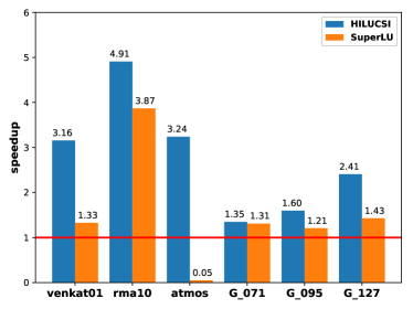
(a) Relative speedup of factorization time.

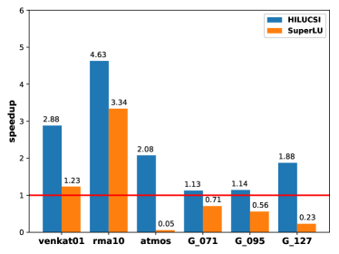
(b) Relative speedup of total time.

Figure 2: Speedups of (a) factorization and (b) total times of HILUCSI and SuperLU versus ILUPACK for nearly symmetric, indefinite problems with optimized parameters. Higher is better. In the horizontal axis, “atmos” and “G_” are short for atmosmodl and Goodwin_ in the horizontal axis, respectively.

We observe that although SuperLU outperformed ILUPACK in terms of factorization times for all the Goodwin problems, it underperformed in terms of the overall times for these problems, due to the slow convergence of GMRES. This result again shows the superior robustness of MLILU in HILUCSI and ILUPACK versus the single-level ILUTP in SuperLU.

4.2.2 Symmetric saddle-point problems.

We now assess the robustness and efficiency of HILUCSI as the problem sizes increase. To this end, we use the symmetric saddle-point problems and compare HILUCSI with two different solvers in ILUPACK for symmetric and unsymmetric matrices, respectively. Because supernodal ILUTP failed for most of these problems, we do not include it in this comparison. For these saddle-point problems, because there are static deferring, our algorithm enabled symmetric matching in HILUCSI on the first two levels, and we applied RCM for the first level and applied AMD ordering for all the other levels. For ILUPACK, we used AMD ordering, as recommended by ILUPACK’s documentation.

Table 3 shows the comparison of HILUCSI with ILUPACK in terms of the numbers of GMRES iterations, the nonzero ratios, and the numbers of levels, along with the runtimes of HILUCSI. It is worth noting that symmetric ILUPACK failed for the two larger systems for the Stokes equations due to encountering a structurally singular system during preprocessing. For the two larger cases for the mixed formulation of the Poisson equation, symmetric ILUPACK was notably less robust and required many more GMRES iterations. Among the four solved problems, symmetric ILUPACK improved the runtimes of unsymmetric ILUPACK by a factor of 1.2 to 2.6, because the symmetric version performed computations only on the lower triangular part and used different dropping strategies.

Remark 5.

The results of unsymmetric versus symmetric ILUPACK in Table 3 show that it is sometimes more robust to solve symmetric indefinite systems using unsymmetric solvers. Conventionally, it is believed that “it is rarely sensible to throw away symmetry in preconditioning” [42]. Such conventional wisdom seems to focus on the efficiency of single-level ILU, because it may reduce the computational cost by up to half by using symmetric (versus unsymmetric) factorization [84, 24]. The use of unsymmetric factorization at the coarse levels in HILUCSI is a crucial reason for its robustness for symmetric saddle-point problems.

Table 3: Comparison of HILUCSI (denoted as H) with unsymmetric and symmetric ILUPACK (denoted by IU and IS, respectively) for symmetric saddle-point systems with droptol $10^{-2}$ for all and $\alpha=3$ for HILUCSI. $\times$ indicates failed factorization.

Matrix	HILUCSI		GMRES iters.			nnz ratio			#levels
	factor.	total	H	IU	IS	H	IU	IS	H	IU	IS
S3D1	0.44	0.45	4	3	7	2.0	4.6	6.4	3	6	5
S3D2	5.56	5.83	7	3	$\times$	2.5	6.3	$\times$	3	6	$\times$
S3D3	61.7	64.1	7	4	$\times$	2.7	8.4	$\times$	4	9	$\times$
M3D1	0.69	0.78	14	6	11	2.7	7.9	5.8	4	8	5
M3D2	6.25	7.75	26	11	29	2.6	9.5	7.3	5	10	5
M3D3	52.9	76.8	53	24	62	2.6	10	7.2	6	15	5

In terms of efficiency, Figure 3 shows the relative speedups of HILUCSI and symmetric ILUPACK relative to the unsymmetric ILUPACK. It can be seen that HILUCSI outperformed the unsymmetric ILUPACK by a factor of four to ten for these problems. The improvement was mostly due to the improved dropping in HILUCSI. HILUCSI also had fewer levels than unsymmetric ILUPACK. Note that the timing results in Table 3 for HILUCSI did not use symmetric factorization at any level. The use of symmetric factorization in the first two levels further improved its overall performance by 10–20%. Note that in Figure 3, the relative speedup of HILUCSI versus ILUPACK grew as the problem sizes increased. Hence, the better efficiency of HILUCSI for large-scale systems is primarily due to its better scalability with respect to problem sizes, thanks to its scalability-oriented dropping.

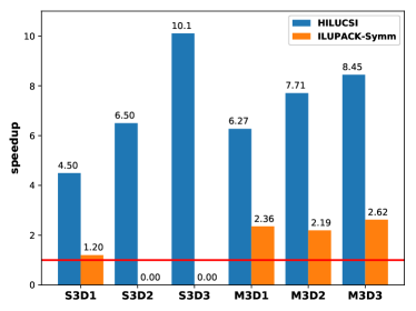
(a) Relative speedup of factorization time.

(b) Relative speedup of total time.

Figure 3: Speedups of (a) factorization and (b) total times of HILUCSI and symmetric factorization in ILUPACK versus unsymmetric ILUPACK for symmetric saddle-point problems. Higher is better.

4.3 Benefits of mixed preprocessing

To assess the effectiveness of mixing symmetric and unsymmetric preprocessing for HILUCSI as we described in Section 3.3, we applied symmetric preprocessing on zero, one, and two levels. Table 4 shows a comparison of the factorization times, total times, GMRES iterations, and nnz ratios for three different classes of problems. It can be seen that for matrices with fully unsymmetric structures, the use of symmetric preprocessing did not improve robustness and even decreased efficiency. However, for many unsymmetric matrices with nearly symmetric structures, using symmetric preprocessing on the first level significantly improved robustness and efficiency. The behavior is probably because the matrices from systems of PDEs tend to have some block diagonal dominance as defined in [93], which may be destroyed by unsymmetric permutations. Symmetric reordering and equilibration permute the dominant block diagonal within a narrower band, so that it may preserve block diagonal dominance more effectively. Furthermore, when static deferring is invoked in (nearly) symmetric saddle-point problems, using two levels of symmetric preprocessing further reduced the factorization times, but the total runtime remained about the same.

Table 4: Effect of mixing symmetric and unsymmetric processing in HILUCSI. H0, H1, and H2 denote using zero, one, and two levels of symmetric preprocessing.

Matrix	factor. time			total time			GMRES iters.			nnz ratio
	H0	H1	H2	H0	H1	H2	H0	H1	H2	H0	H1	H2
general unsymmetric systems
bbmat	31.4	45.5	55.2	31.9	46.3	55.9	9	11	9	17	25	32
nearly symmetric systems
rma10	4.85	2.31	2.53	5.02	2.47	2.69	67	9	9	3.4	2.0	2.3
PR02R	$-$	256	293	$-$	261	300	$-$	14	15	$-$	28	32
symmetric, saddle-point problems
M3D3	$-$	53.6	52.9	$-$	77.3	76.8	$-$	52	53	$-$	2.6	2.6
M3D2	8.06	6.37	6.25	16.1	7.69	7.75	120	23	26	4.0	2.6	2.6

5 Conclusions and Future Work

In this paper, we described an MLILU technique, called HILUCSI, which is designed for saddle-point problems from PDEs. The key novelty of HILUCSI is that it takes into account the near or partial symmetry of the underlying problems, and it improves the simplicity, robustness, and efficiency of MLILU. More specifically, HILUCSI applies static and dynamic deferring for improving robustness while enjoying a simpler implementation than pivoting. It applies symmetric preprocessing techniques at the top level for nearly or partially symmetric systems but applies unsymmetric preprocessing and factorization at coarser levels, which improved the robustness for problems from systems of PDEs. Furthermore, the scalability-oriented dropping significantly improved the efficiency of MLILU for large-scale problems. We demonstrated the robustness and efficiency of HILUCSI as a right-preconditioner of restarted GMRES for symmetric and unsymmetric saddle-point problems from mixed Poisson, Stokes, and Navier-Stokes equations. Our results showed that HILUCSI is significantly more robust than single-level ILU, such as SuperLU. It also outperforms other MLILU packages (specifically, ILUPACK) by a factor of four to ten for medium to large problems.

In its current form, HILUCSI has several limitations. First, if the memory is severely limited, there may be too many droppings or too many levels, and the preconditioner may lose robustness and efficiency. We plan to optimize HILUCSI further for limited-memory situations. Second, for vector-valued PDEs, the matrices may exhibit block structures. It may be worthwhile to explore such block structures to improve cache performance, similar to that in [6] and [46]. Finally, the HILUCSI algorithm is sequential as presented in this paper. We will report its parallelization in the future.

Appendix A Thresholding in inverse-based dropping

We motivate our thresholding strategy in inverse-based dropping within each level of HILUCSI, based on a heuristic stability analysis to bound $\rho\left(\boldsymbol{A}\boldsymbol{M}^{-1}-\boldsymbol{I}\right)$ (i.e., using the spectral radius as a “pseudo-norm” of $\boldsymbol{A}\boldsymbol{M}^{-1}-\boldsymbol{I}$). Let $\boldsymbol{\delta}_{A}=\boldsymbol{A}-\boldsymbol{M}$, where $\boldsymbol{M}=\boldsymbol{L}\boldsymbol{D}\boldsymbol{U}$, and $\boldsymbol{A}=\left(\boldsymbol{L}+\boldsymbol{\delta}_{L}\right)\left(\boldsymbol{D}+\boldsymbol{\delta}_{D}\right)\left(\boldsymbol{U}+\boldsymbol{\delta}_{U}\right)$, where $\boldsymbol{\delta}_{L}$, $\boldsymbol{\delta}_{D}$, and $\boldsymbol{\delta}_{U}$ denote the perturbations to $\boldsymbol{L}$, $\boldsymbol{D}$, and $\boldsymbol{U}$, respectively. Hence,

$$\boldsymbol{\delta}_{A} =\left(\boldsymbol{L}+\boldsymbol{\delta}_{L}\right)\left(\boldsymbol{D}+\boldsymbol{\delta}_{D}\right)\left(\boldsymbol{U}+\boldsymbol{\delta}_{U}\right)-\boldsymbol{L}\boldsymbol{D}\boldsymbol{U}$$

$$=\boldsymbol{\delta}_{L}\boldsymbol{D}\boldsymbol{U}+\boldsymbol{L}\boldsymbol{\delta}_{D}\boldsymbol{U}+\boldsymbol{L}\boldsymbol{D}\boldsymbol{\delta}_{U}+\text{h.o.t.},$$

where we omit the higher-order terms that involve more than one $\boldsymbol{\delta}$ matrix. Note that

$$\rho\left(\boldsymbol{A}\boldsymbol{M}^{-1}-\boldsymbol{I}\right) =\rho\left(\sqrt{\boldsymbol{D}^{-1}}\boldsymbol{L}^{-1}\boldsymbol{\delta}_{A}\boldsymbol{M}^{-1}\boldsymbol{L}\sqrt{\boldsymbol{D}}\right)$$

$$\approx\rho\left(\sqrt{\boldsymbol{D}^{-1}}\left(\boldsymbol{L}^{-1}\boldsymbol{\delta}_{L}+\boldsymbol{\delta}_{D}\boldsymbol{D}^{-1}\right)\sqrt{\boldsymbol{D}}+\sqrt{D}\boldsymbol{\delta}_{U}\boldsymbol{U}^{-1}\sqrt{\boldsymbol{D}^{-1}}\right)$$

$$\leq\sqrt{\kappa(\boldsymbol{D})}\left(\left\|\boldsymbol{L}^{-1}\boldsymbol{\delta}_{L}\right\|+\left\|\boldsymbol{\delta}_{D}\boldsymbol{D}^{-1}\right\|+\left\|\boldsymbol{\delta}_{U}\boldsymbol{U}^{-1}\right\|\right).$$ (10)

In dynamic deferring, we restrict the magnitude of the diagonal entries to be no smaller than $1/\kappa_{D}$, and we estimate the maximum magnitudes to be approximately equal to $\kappa_{D}$. Hence, $\sqrt{\kappa(\boldsymbol{D})}$ is bounded by $\kappa_{D}$, which leads to our thresholding for inverse-based dropping in Section 3.1. In terms of $\boldsymbol{L}^{-1}\boldsymbol{\delta}_{L}$ and $\boldsymbol{\delta}_{U}\boldsymbol{U}^{-1}$, it is difficult to bound their 2-norms, and hence we approximately bound $\left\|\boldsymbol{L}^{-1}\boldsymbol{\delta}_{L}\right\|_{\infty}$ and $\left\|\boldsymbol{\delta}_{U}\boldsymbol{U}^{-1}\right\|_{1}$ by $\left\|\boldsymbol{L}^{-1}\right\|_{\infty}\left\|\boldsymbol{\delta}_{L}\right\|_{\infty}$ and $\left\|\boldsymbol{U}^{-1}\right\|_{1}\left\|\boldsymbol{\delta}_{U}\right\|_{1}$, respectively, as in [26] and [25]. However, note that the thresholding strategy in [26] and [25] did not take into account $\sqrt{\kappa(\boldsymbol{D})}$ (or $\kappa_{D}$). This omission was because they derived the thresholds based on bounding $\boldsymbol{L}^{-1}\boldsymbol{A}\boldsymbol{U}^{-1}-\boldsymbol{D}$ instead of $\boldsymbol{A}\boldsymbol{M}^{-1}-\boldsymbol{I}$, probably because it is impractical to bound $\boldsymbol{A}\boldsymbol{M}^{-1}-\boldsymbol{I}$ in a single-level ILU. In contrast, our derivation is for each level of MLILU with dynamic deferring, so it is practical to bound some norm of $\boldsymbol{A}\boldsymbol{M}^{-1}-\boldsymbol{I}$, which corresponds to a stability measure of ILU [39].

Appendix B Linear time complexity within each level

For linear systems arising from PDEs, the input matrix $\boldsymbol{A}\in\mathbb{R}^{n\times n}$ typically has a constant number of nonzeros per row and per column. We now show that the total cost of HILUCSI is linear in $n$ within each level in this setting.

Let us analyze the cost of the first level in detail. Let $\boldsymbol{P}\in\mathbb{N}^{n\times n}$, $\boldsymbol{Q}\in\mathbb{N}^{n\times n}$, $\boldsymbol{L}\in\mathbb{R}^{n\times m}$, $\boldsymbol{D}\in\mathbb{R}^{m\times m}$ and $\boldsymbol{U}\in\mathbb{R}^{m\times n}$ be the output of the factorization of the current level. First, let us consider the cost of updating $\boldsymbol{\ell}_{k}$ and $\boldsymbol{u}_{k}^{T}$ using the Crout version of ILU, or in short, Crout update. The total number of floating-point operations is bounded by

$$\mathcal{O}\left(\text{nnz}\left(\boldsymbol{L}+\boldsymbol{U}\right)\left(\max_{i\leq m}\left\{\text{nnz}\left(\boldsymbol{a}_{i}^{T}\right)\right\}+\max_{j\leq m}\left\{\text{nnz}\left(\boldsymbol{a}_{j}\right)\right\}\right)\right),$$ (11)

where $\boldsymbol{a}_{i}^{T}$ and $\boldsymbol{a}_{j}$ denote the $i$th row and $j$th column of $\boldsymbol{P}^{T}\boldsymbol{A}\boldsymbol{Q}$, respectively. Second, let us consider the cost of deferring and dropping. Given an efficient data structure (see Section 3.2), the number of floating-point operations in dynamic deferring is proportional to Crout update. Furthermore, in the scalability-oriented dropping, we use quick select, which has an expected linear time complexity, to find the largest nonzeros, followed by quick sort after dropping. Hence, the time complexity of dropping is lower than that of Crout update. If there is a constant number of nonzeros in each row and column, then

$$\max_{i\leq n}\left\{\text{nnz}\left(\boldsymbol{a}_{i}^{T}\right)\right\}+\max_{j\leq n}\left\{\text{nnz}\left(\boldsymbol{a}_{j}\right)\right\}=\mathcal{O}(1),$$

and $\text{nnz}\left(\boldsymbol{L}+\boldsymbol{U}\right)=\text{nnz}\left(\boldsymbol{A}\right)=\mathcal{O}(n)$. Hence, Crout update with deferring takes linear time. Third, for the Schur component in 4, the most expensive and also the most challenging part is the computation of $\boldsymbol{L}_{E}\boldsymbol{D}_{B}\boldsymbol{U}_{F}$. We compute $\boldsymbol{L}_{E}$ and $\boldsymbol{U}_{F}$ along with $\boldsymbol{L}_{B}$ and $\boldsymbol{U}_{B}$ during Crout update, so its cost is bounded by (11). We compute the sparse matrix-matrix multiplication (SpMM) using the algorithm as described in [94]. Since our scalability-oriented dropping ensures that the nonzeros in each row of $\boldsymbol{L}_{E}$ and in each column of $\boldsymbol{U}_{F}$ are bounded by a constant factor of those in the input matrix (see Section 3.1), the SpMM also takes linear time. As a side product, nnz of $\boldsymbol{S}_{C}$ is linear in that of $\boldsymbol{A}$.

For the other levels, the analysis described above also applies by considering the fact that the nnz in the present level is proportional to that in $\boldsymbol{A}$, and that the scalability-oriented dropping is performed based on the nnz in each row and column in the input matrix.

References

- [1] Saad Y. Iterative Methods for Sparse Linear Systems. 2nd edn., SIAM, 2003.
- [2] Saad Y, Schultz M. GMRES: A generalized minimal residual algorithm for solving nonsymmetric linear systems. SIAM J. Sci. Stat. Comput. 1986; 7(3):856–869.
- [3] van der Vorst HA. Bi-CGSTAB: A fast and smoothly converging variant of Bi-CG for the solution of nonsymmetric linear systems. SIAM J. Sci. Stat. Comput. 1992; 13(2):631–644.
- [4] Chow E, Saad Y. Experimental study of ILU preconditioners for indefinite matrices. J. Comput. Appl. Math. 1997; 86(2):387–414.
- [5] Ernst OG, Gander MJ. Why it is difficult to solve Helmholtz problems with classical iterative methods. Numerical Analysis of Multiscale Problems. Springer, 2012; 325–363.
- [6] Li XS, Shao M. A supernodal approach to incomplete LU factorization with partial pivoting. ACM Trans. Math. Softw. 2011; 37(4).
- [7] Zhu Y, Sameh AH. How to generate effective block Jacobi preconditioners for solving large sparse linear systems. Advances in Computational Fluid-Structure Interaction and Flow Simulation. Springer, 2016; 231–244.
- [8] Bollhöfer M, Saad Y. Multilevel preconditioners constructed from inverse-based ILUs. SIAM J. Sci. Comput. 2006; 27(5):1627–1650.
- [9] Bank RE, Wagner C. Multilevel ILU decomposition. Numer. Math. 1999; 82(4):543–576.
- [10] Saad Y. Multilevel ILU with reorderings for diagonal dominance. SIAM J. Sci. Comput. 2005; 27(3):1032–1057.
- [11] Vassilevski PS. Multilevel Block Factorization Preconditioners: Matrix-Based Analysis and Algorithms for Solving Finite Element Equations. Springer, 2008.
- [12] Ghai A, Lu C, Jiao X. A comparison of preconditioned Krylov subspace methods for large-scale nonsymmetric linear systems. Numer. Linear Algebra Appl. 2017; :e2215.
- [13] Bollhöfer M, Aliaga JI, Martın AF, Quintana-Ortí ES. ILUPACK. Encyclopedia of Parallel Computing. Springer, 2011.
- [14] The HYPRE Team. hypre High-Performance Preconditioners User’s Manual 2017. Version 2.12.2.
- [15] LeVeque RJ. Finite Difference Methods for Ordinary and Partial Differential Equations: Steady State and Time Dependent Problems. SIAM: Philadelphia, 2007.
- [16] Ciarlet PG. The Finite Element Method for Elliptic Problems. SIAM, 2002.
- [17] Ern A, Guermond JL. Theory and Practice of Finite Elements, vol. 159. Springer, 2013.
- [18] LeVeque RJ. Finite Volume Methods for Hyperbolic Problems, vol. 31. Cambridge University Press, 2002.
- [19] Elman HC, Silvester DJ, Wathen AJ. Finite elements and fast iterative solvers: with applications in incompressible fluid dynamics. Oxford University Press, 2014.
- [20] Cheung J, Perego M, Bochev P, Gunzburger M. Optimally accurate higher-order finite element methods for polytopial approximations of domains with smooth boundaries. Math. Comput. 2019; 88(319):2187–2219.
- [21] Johansen H, Colella P. A Cartesian grid embedded boundary method for Poisson’s equation on irregular domains. J. Comput. Phys. 1998; 147(1):60–85.
- [22] Peskin CS. The immersed boundary method. Acta Numerica 2002; 11:479–517.
- [23] Amestoy PR, Duff IS, L’Excellent JY, Koster J. MUMPS: a general purpose distributed memory sparse solver. International Workshop on Applied Parallel Computing, Springer, 2000; 121–130.
- [24] Schenk O, Gärtner K. Parallel sparse direct solver PARDISO – user guide version 6.0.0 2018.
- [25] Li N, Saad Y, Chow E. Crout versions of ILU for general sparse matrices. SIAM J. Sci. Comput. 2003; 25(2):716–728.
- [26] Bollhöfer M. A robust ILU with pivoting based on monitoring the growth of the inverse factors. Linear Algebra Appl. 2001; 338(1-3):201–218.
- [27] Bollhöfer M, Saad Y. On the relations between ILUs and factored approximate inverses. SIAM J. Matrix Anal. Appl. 2002; 24(1):219–237.
- [28] Concus P, Golub GH. A generalized conjugate gradient method for nonsymmetric systems of linear equations. Computing Methods in Applied Sciences and Engineering. Springer, 1976; 56–65.
- [29] Widlund O. A Lanczos method for a class of nonsymmetric systems of linear equations. SIAM J. Numer. Ana. 1978; 15(4):801–812.
- [30] Aksoylu B, Klie H. A family of physics-based preconditioners for solving elliptic equations on highly heterogeneous media. Appl. Numer. Math. 2009; 59(6):1159–1186.
- [31] Benzi M, Golub GH, Liesen J. Numerical solution of saddle point problems. Acta Numerica 4 2005; 14:1–137.
- [32] Bunch JR, Kaufman L. Some stable methods for calculating inertia and solving symmetric linear systems. Math. Comput. 1977; 31(137):163–179.
- [33] Golub GH, Van Loan CF. Matrix Computations. 4th edn., Johns Hopkins, 2013.
- [34] Greif C, He S, Liu P. SYM-ILDL: Incomplete factorization of symmetric indefinite and skew-symmetric matrices. ACM Trans. Math. Softw. 2017; 44(1):1–21.
- [35] Li N, Saad Y. Crout versions of ILU factorization with pivoting for sparse symmetric matrices. Electron. T. Numer. Ana. 2005; 20:75–85.
- [36] Schenk O, Bollhöfer M, Römer RA. On large-scale diagonalization techniques for the Anderson model of localization. SIAM Rev. 2008; 50(1):91–112.
- [37] Saad Y. ILUT: A dual threshold incomplete LU factorization. Numer. Linear Algebra Appl. 1994; 1.
- [38] Lin CJ, Moré JJ. Incomplete Cholesky factorizations with limited memory. SIAM J. Sci. Comput. 1999; 21(1):24–45.
- [39] Benzi M. Preconditioning techniques for large linear systems: a survey. J. Comput. Phys. 2002; 182(2):418–477.
- [40] Chan TF, Van Der Vorst HA. Approximate and incomplete factorizations. Parallel Numerical Algorithms. Springer, 1997; 167–202.
- [41] Saad Y, Van Der Vorst HA. Iterative solution of linear systems in the 20th century. Numerical Analysis: Historical Developments in the 20th Century. Elsevier, 2001; 175–207.
- [42] Wathen AJ. Preconditioning. Acta Numerica 2015; 24:329–376.
- [43] van der Vorst HA. Iterative Krylov Methods for Large Linear Systems, vol. 13. Cambridge University Press, 2003.
- [44] Varga RS. Factorization and normalized iterative methods. Technical Report, Westinghouse Electric Corp., Pittsburgh 1959.
- [45] Meijerink JA, van der Vorst HA. An iterative solution method for linear systems of which the coefficient matrix is a symmetric M-matrix. Math. Comput. 1977; 31(137):148–162.
- [46] Gupta A, George T. Adaptive techniques for improving the performance of incomplete factorization preconditioning. SIAM J. Sci. Comput. 2010; 32(1):84–110.
- [47] Jones MT, Plassmann PE. An improved incomplete Cholesky factorization. ACM Trans. Math. Softw. 1995; 21(1):5–17.
- [48] Simon HD, et al.. Incomplete LU preconditioners for conjugate-gradient-type iterative methods. SPE Reservoir Engineering 1988; 3(01):302–306.
- [49] Bollhöfer M. A robust and efficient ILU that incorporates the growth of the inverse triangular factors. SIAM J. Sci. Comput. 2003; 25(1):86–103.
- [50] Mayer J. Alternative weighted dropping strategies for ILUTP. SIAM J. Sci. Comput. 2006; 27(4):1424–1437.
- [51] Balay S, Abhyankar S, Adams MF, Brown J, Brune P, Buschelman K, Dalcin L, Eijkhout V, Gropp WD, Kaushik D, et al.. PETSc Users Manual. Technical Report ANL-95/11 - Revision 3.7, Argonne National Laboratory 2016.
- [52] Saad Y. Preconditioning techniques for nonsymmetric and indefinite linear systems. J. Comput. Appl. Math. 1988; 24:89–105.
- [53] The MathWorks, Inc. MATLAB R2019a. Natick, MA 2019.
- [54] Saad Y. SPARSEKIT: a basic toolkit for sparse matrix computations. Technical Report, University of Minnesota 1994.
- [55] Li XS. An overview of SuperLU: Algorithms, implementation, and user interface. ACM Trans. Math. Softw. 2005; 31(3):302–325.
- [56] Mayer J. A multilevel Crout ILU preconditioner with pivoting and row permutation. Numer. Linear Algebra Appl. 2007; 14:771–789.
- [57] Eisenstat SC, Schultz MH, Sherman AH. Algorithms and data structures for sparse symmetric Gaussian elimination. SIAM J. Sci. Stat. Comp. 1981; 2(2):225–237.
- [58] Chan WM, George A. A linear time implementation of the reverse Cuthill-McKee algorithm. BIT Numer. Math. 1980; 20(1):8–14.
- [59] Amestoy PR, Davis TA, Duff IS. An approximate minimum degree ordering algorithm. SIAM J. Matrix Anal. Appl. 1996; 17(4):886–905.
- [60] Dupont T, Kendall RP, Rachford H Jr. An approximate factorization procedure for solving self-adjoint elliptic difference equations. SIAM J. Num. Anal. 1968; 5(3):559–573.
- [61] Gustafsson I. A class of first order factorization methods. IT Numer. Math. 1978; 18(2):142–156.
- [62] Elman HC. A stability analysis of incomplete LU factorizations. Math. Comput. 1986; :191–217.
- [63] van der Sluis A. Condition numbers and equilibration of matrices. Numer. Math. 1969; 14:14–23.
- [64] Golub GH, Van Loan CF. Matrix Computations, vol. 3. JHU Press, 2012.
- [65] Saad Y. ILUM: a multi-elimination ILU preconditioner for general sparse matrices. SIAM J. Sci. Comput. 1996; 17(4):830–847.
- [66] Saad Y, Zhang J. BILUTM: a domain-based multilevel block ILUT preconditioner for general sparse matrices. SIAM J. Matrix Anal. Appl. 1999; 21(1):279–299.
- [67] Saad Y, Suchomel B. ARMS: An algebraic recursive multilevel solver for general sparse linear systems. Numer. Linear Algebra Appl. 2002; 9(5):359–378.
- [68] Zhang J. A multilevel dual reordering strategy for robust incomplete LU factorization of indefinite matrices. SIAM J. Matrix Anal. Appl. 2001; 22(3):925–947.
- [69] Mayer J. ILU++: A new software package for solving sparse linear systems with iterative methods. PAMM: Proceedings in Applied Mathematics and Mechanics 2007; 7(1):2020 123–2020 124.
- [70] MacLachlan S, Saad Y. Greedy coarsening strategies for nonsymmetric problems. SIAM J. Sci. Comput. 2007; 29(5):2115–2143.
- [71] Osei-Kuffuor D, Li R, Saad Y. Matrix reordering using multilevel graph coarsening for ILU preconditioning. SIAM J. Sci. Comput. 2015; 37(1):A391–A419.
- [72] Bank RE, Smith RK. The incomplete factorization multigraph algorithm. SIAM J. Sci. Comput. 1999; 20(4):1349–1364.
- [73] Bank RE, Xu J. The hierarchical basis multigrid method and incomplete LU decomposition. Contemporary Mathematics 1994; 180:163–173.
- [74] Tismenetsky M. A new preconditioning technique for solving large sparse linear systems. Linear Algebra Appl. 1991; 154(331–353).
- [75] Hackbusch W. Hierarchical Matrices: Algorithms and Analysis, vol. 49. Springer, 2015.
- [76] Ruge JW, Stüben K. Multigrid methods, chap. Algebraic multigrid. SIAM, 1987; 73–130.
- [77] Axelsson O, Vassilevski PS. Algebraic multilevel preconditioning methods, II. SIAM J. Numer. Ana. 1990; 27(6):1569–1590.
- [78] Higham NJ. A survey of condition number estimation for triangular matrices. SIAM Review 1987; 29:575–596.
- [79] Mayer J. ILUCP: a Crout ILU preconditioner with pivoting. Numer. Linear Algebra Appl. 2005; 12(9):941–955.
- [80] Duff IS, Koster J. The design and use of algorithms for permuting large entries to the diagonal of sparse matrices. SIAM J. Matrix Anal. Appl. 1999; 20(4):889–901.
- [81] Duff IS, Koster J. On algorithms for permuting large entries to the diagonal of a sparse matrix. SIAM J. Matrix Anal. Appl. 2001; 22(4):973–996.
- [82] Benzi M, Szyld DB, Van Duin A. Orderings for incomplete factorization preconditioning of nonsymmetric problems. SIAM J. Sci. Comput. 1999; 20(5):1652–1670.
- [83] Laboratory SRA. HSL_MC64 version 2.3.1: Permute and scale a sparse unsymmetric or rectangular matrix to put large entries on the diagonal 2013. Http://www.hsl.rl.ac.uk/catalogue/hsl_mc64.html.
- [84] Duff IS, Pralet S. Strategies for scaling and pivoting for sparse symmetric indefinite problems. SIAM J. Matrix Ana. Appl. 2005; 27(2):313–340.
- [85] Heggernes P, Eisenstat S, Kumfert G, Pothen A. The computational complexity of the minimum degree algorithm. Proceedings of 14th Norwegian Computer Science Conference, 2001; 98–109.
- [86] Bollhöfer M, Saad Y. ILUPACK preconditioning software package 2011. Available online at http://ilupack.tu-bs.de/. Release V2.4, June.
- [87] Davis TA, Hu Y. The University of Florida sparse matrix collection. ACM Trans. Math. Softw. 2011; 38(1):1.
- [88] Boisvert RF, Pozo R, Remington K, Barrett RF, Dongarra JJ. Matrix Market: a web resource for test matrix collections. Qual. Numer. Softw.. Springer, 1997; 125–137.
- [89] Alnæs M, Blechta J, Hake J, Johansson A, Kehlet B, Logg A, Richardson C, Ring J, Rognes ME, Wells GN. The FEniCS project version 1.5. Arc. Num. Softw. 2015; 3(100):9–23.
- [90] Taylor C, Hood P. A numerical solution of the Navier-Stokes equations using the finite element technique. Computers & Fluids 1973; 1(1):73–100.
- [91] Brezzi F, Douglas J, Marini LD. Two families of mixed finite elements for second order elliptic problems. Numer. Math. 1985; 47(2):217–235.
- [92] Cockburn B, Karniadakis GE, Shu CW. The Development of Discontinuous Galerkin Methods. Springer: Berlin Heidelberg, 2000.
- [93] Feingold DG, Varga RS, et al.. Block diagonally dominant matrices and generalizations of the Gerschgorin circle theorem. Pac. J. Math. 1962; 12(4):1241–1250.
- [94] Bank RE, Douglas CC. Sparse Matrix Multiplication Package (SMMP). IBM Thomas J. Watson Research Division, 1992.