An introductory guide to aligning networks using SANA, the Simulated Annealing Network Aligner

Abstract

Sequence alignment has had an enormous impact on our understanding of biology, evolution, and disease. The alignment of biological networks holds similar promise. Biological networks generally model interactions between biomolecules such as proteins, genes, metabolites, or mRNAs. There is strong evidence that the network topology— the “structure” of the network—is correlated with the functions performed, so that network topology can be used to help predict or understand function. However, unlike sequence comparison and alignment—which is an essentially solved problem—network comparison and alignment is an NP-complete problem for which heuristic algorithms must be used.

Here we introduce SANA, the Simulated Annealing Network Aligner. SANA is one of many algorithms proposed for the arena of biological network alignment. In the context of global network alignment, SANA stands out for its speed, memory efficiency, ease-of-use, and flexibility in the arena of producing alignments between 2 or more networks. SANA produces better alignments in minutes on a laptop than most other algorithms can produce in hours or days of CPU time on large server-class machines. We walk the user through how to use SANA for several types of biomolecular networks.

Availability: https://github.com/waynebhayes/sana

Contact: whayes@uci.edu

Supplementary information: Available online.

1 Introduction

A biological network consists of a set of nodes representing entities, with edges connecting entities that are related in some way. They come in many varieties, such as protein-protein interaction (PPI) networks (Williamson and Sutcliffe, 2010; Jaenicke and Helmreich, 2012), gene regulatory networks (Davidson, 2010; Karlebach and Shamir, 2008), gene-$\mu$RNA networks (Chen and Rajewsky, 2007; Prescott, 2012; Farazi et al., 2013; Kotlyar et al., 2015; Tokar et al., 2017), metabolic networks (Fiehn, 2002), brain connectomes (Milano et al., 2017), and many others (Junker and Schreiber, 2011). It is believed that the structure of the networks, in the form of the network topology, is related to the function of the entities (Davidson, 2010; Davis et al., 2015; Sporns, 2010). The alignment of such networks aims to use connectivity between nodes—the topology of the network—to aid extraction of information about the nodes and their function. Network alignments can be used to build taxonomic trees and find highly conserved pathways across distant species (Kuchaiev et al., 2010); and by extension finding such topological similarities may aid in transfering functional knowledge from better-understood species to less well-understood ones, much like how sequence alignment has been doing so for sequence for decades. Networks are even starting to have an influence on individual human health (Van El et al., 2013)

Network alignment is a fundamentally difficult problem: it is a generalization of the NP-Complete subgraph isomorphism problem (Cook, 1971; Garey and Johnson, 1979); and adding to the difficulty is that current data sets are very noisy (Von Mering et al., 2002). Therefore, modern alignment algorithms try to approximate solutions using heuristic approaches.

There are several sub-classes of network alignment. Global Network Alignment (GNA) is the task of attempting to completely align entire networks to each other; GNA applied to just two networks is called pairwise GNA (Kuchaiev et al., 2010; Malod-Dognin and Pržulj, 2015; Saraph and Milenković, 2014; Mamano and Hayes, 2017; Hashemifar and Xu, 2014; Sun et al., 2015; Patro and Kingsford, 2012), while aligning more than two whole networks is called multiple GNA. In contrast, Local Network Alignment (LNA) attempts to find similarity in the local wiring patterns among small groups of nodes, either in the same network, or across many networks. In all of these cases, alignments can map nodes 1-to-1, or many-to-many; the latter is more biologically realistic since, for example, one gene in yeast may have multiple homologs in mammals. However, the 1-to-1 assumption makes programming simpler and so the majority of aligners take the 1-to-1 mapping as a simplifying assumption. A more recent version of network alignment looks into modeling dynamic networks (see for example Vijayan and Milenković (2017)). An excellent comprehensive survey of all these types of alignments is provided by Faisal et al. (2015a). SANA was originally a 1-to-1 pairwise global network alignment algorithm, although we here also introduce a prototype multiple network alignment version.

1.1 User/System requirements

Source code to SANA is available on GitHub at

http://github.com/waynebhayes/SANA, and is best cloned from github on the Unix command line using

git clone http://github.com/waynebhayes/SANA

SANA is written in C++ and runs best on the Unix command line. It has been tested with gcc 4.8, 4.9, 5.2, and 5.4, and runs on Unix, Linux, Mac OS/X, and under the Windows-based Unix emulator Cygwin (http://cygwin.com), 32-bit or 64-bit. SANA has a rudimentary Web interface at http://sana.ics.uci.edu, and a rudimentary SANA app is available in the Cytoscape app store. SANA expects its input networks to be in a two-column ASCII format we call edge list format: each line is one edge, specified by listing the two nodes at each end of the edge in arbitrary order (unless -nodes-have-types is specified, see below). Duplicate edges and self-loops are not allowed. We also supply a program called createEdgeList that can convert the following types of formats into SANA’s edgeList format: XML, GML, LEDA, .gw, CSV, LGF.

1.2 Alignment measures & objective functions

An alignment measure is any quantity designed to evaluate the quality of a network alignment. Alignment measures can be classified along many axes.

1.2.1 Objective vs. non-objective measures.

The first axis is the distinction between objectives and what we call post-hoc measures. While both can be evaluated on any given alignment, any measure used to guide an alignment as it is being created is called an objective function; any measure not used to guide the alignment is generally applied after-the-fact as an independent measure of quality. A good alignment algorithm should be able to use virtually any measure as an objective, and also evaluate the alignment after-the-fact using any other measures which were not used as objectives.

1.2.2 Graph topology vs. biological measures.

Another axis along which measures can be classified is topological vs biological.

A topological measure

quantifies a network alignment based solely on graph-theoretic grounds. Several such measures exist: $EC$ (Kuchaiev et al., 2010), $ICS$ (Patro and Kingsford, 2012), and $S^{3}$ (Saraph and Milenković, 2014) quantify the number of edges in one network that are mapped to edges in the other network(s); they are all described in more detail below. Other topological measures use graphlets to quantify local structure (Pržulj et al., 2004b; Milenković and Pržulj, 2008; Yaveroğlu et al., 2014; Malod-Dognin and Pržulj, 2015), while still others use graph measures such as spectral analysis (Patro and Kingsford, 2012) and degree similarity-based measures such as Importance (Hashemifar and Xu, 2014).

Biological measures.

In contrast, biological measures are usually used to compare the nodes from different networks that have been paired together by the alignment. For genes or proteins, a common measure is the sequence similarity or BLAST score between the aligned nodes (Camacho et al., 2009); sequence similarity is also frequently combined with topology to produce a hybrid objective function (see for example Kuchaiev and Pržulj (2011); Saraph and Milenković (2014); Mamano and Hayes (2017); Malod-Dognin and Pržulj (2015), among many others). Another biology-based measure is the functional similarity between pairs of aligned proteins as expressed by GO (Gene Ontology) terms (Consortium, 2008). While many authors quantify the functional similarity exposed by an alignment using the mean value of various pairwise GO similarity measures across the alignment, such mean-of-pairwise-scores assume each pair of aligned proteins is independent of all others, which is not true in an alignment since every pair is implicitly related to every other pair via the alignment itself. This problem is alleviated by the NetGO score as implemented in SANA (Hayes and Mamano, 2017), which is a global rather than local scoring mechanism (see below for the meaning of local vs. global measures).

1.2.3 Local vs. global measures.

The final axis along which network alignment measures can be classified is what we refer as local vs. global measures.

A local measure

is one that involves evaluating node pairs that are aligned to each other, and has no explicit dependence on the alignment edges and thus has no explicit dependence on network topology. Examples of local measures include sequence similarity and pairwise GO term similarity as described above; some local measures such as graphlet similarity (Kuchaiev et al., 2010; Malod-Dognin and Pržulj, 2015; Saraph and Milenković, 2014) and Importance (Hashemifar and Xu, 2014) include topology indirectly by pre-computing all-by-all pairwise local topological similarities between all pairs of nodes in one network and all pairs of nodes in the other.

Global measures

are ones that implicitly or explicitly can be computed only on the entire alignment and have nothing to do with pairwise node similarities. The most common global measures are $EC$, $ICS$, and $S^{3}$, described in more detail below.

1.3 Major Topological Measures

1.3.1 A useful analogy for topological measures.

In order to more easily understand and discuss topological measures, we introduce an analogy between pairwise network alignment, and the old board game of Battleship. A Battleship game consists of many holes in a board, and some pegs that are placed into the holes. In our analogy, assume $G_{1}$ is a “smaller” network with $n_{1}$ nodes and $m_{1}$ edges, and $G_{2}$ is a “larger” network with $n_{2}$ nodes and $m_{2}$ edges, and we assume that $n_{1}\leq n_{2}$—that is, $G_{1}$ is the smaller network in terms of number of nodes. We will furthermore depict $G_{1}$ as blue and $G_{2}$ as red. Consider Figure 1: this board has $n_{2}=6$ red holes with red edges painted between two holes if there is an edge between the two corresponding nodes in $G_{2}$. The smaller network $G_{1}$ is represented by $n_{1}=4$ blue pegs; edges between the pegs are represented by blue “laser beams” between the corresponding pegs (because laser beams don’t get tangled as pegs are moved from hole to hole). Any placement of the $n_{1}$ pegs into the $n_{2}$ holes represents an alignment between $G_{1}$ and $G_{2}$; for now we assume that each peg is placed into exactly one hole, so that there are exactly $n_{2}-n_{1}$ empty holes. Furthermore, since mixing red and blue creates purple, we depict the alignment (far right of Figure 1) in purple: a blue peg in a red hole is purple, and a blue edge lying on top of a red one is also depicted as purple.

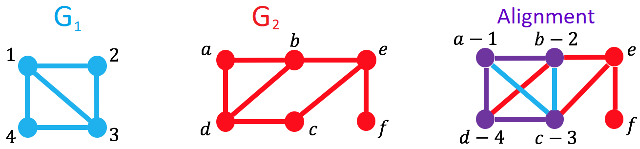
Figure 1: A simple example of a network alignment. The smaller network $G_{1}$ (far left) has its pegs, numbered 1–4, and edges (“laser beams”) depicted in blue; the larger network $G_{2}$ (middle) has its holes and painted edges depicted in red. One possible alignment (in this case the “visually obvious” one) is depicted at the far right. Here, aligned nodes and edges are depicted as purple; unaligned laser beams from $G_{1}$ are still blue, and unaligned holes and edges from $G_{2}$ are still red. As stated in the text, in an alignment figure like the one on the right, the number of edges in $G_{1}$ is always $m_{1}=$(purple + blue edges), and the number of edges in $G_{2}$ is always $m_{2}=$(purple + red edges). Thus, from the figure, it can be easily seen that $EC=3/5$, and $S^{3}=3/6$ (where 6 is the total number of edges visible across all colors on the subgraph induced by the alignment); also $ICS=3/4$, since there are 4 edges induced in $G_{2}$ by the alignment (ie., by purple nodes). The purple network is called the Common Subgraph, and it can consist of several connected components. In this case there is only one Common Connected Subgraph consisting of 4 nodes and 3 edges.

1.3.2 Edge-based measures: $EC,ICS,S^{3}$

We can now define some edge-based topological measures based on this analogy. The fraction of laser beams that lie on top of painted edges is called the $EC$ (Kuchaiev et al., 2010). The numerator of $EC$ is the number of (purple) edges that are aligned between the two networks, call it $AE$ (an integer), while the denominator is $m_{1}$; note that since at most $m_{1}$ edges can be aligned, the value $EC=AE/m_{1}$ is always less than or equal to 1. The authors of MAGNA (Saraph and Milenković, 2014) noted that $EC$ is asymmetric: in particular, if $n_{1}=n_{2}$ then we can “turn the board upside down”, swapping the roles of pegs and holes. In that case, the $EC$ changes because $G_{1}$ and $G_{2}$ are swapped: in particular, the numerator is always the number of aligned edges $AE$, but the denominator switches from $m_{1}$ to $m_{2}$.

The authors of MAGNA fixed the asymmetry of $EC$ by introducing the Symmetric Substructure Score or $S^{3}$. Consider the rightmost section of Figure 1, which depicts a proposed alignment. In our analogy, if we “look down” on the alignment from above, we can see four different types of edges. There are: (i) $AE$ aligned (purple) edges; (ii) $UE_{1}$ unaligned (blue) edges from $G_{1}$; (iii) $UE_{2in}$ unaligned (red) edges in $G_{2}$ induced between purple nodes; and (iv) $UE_{2out}$ unaligned (red) edges outside the alignment (ie., not induced between purple nodes). Note that the following equations always hold: $m_{1}=AE+UE_{1}$ and $m_{2}=AE+UE_{2in}+UE_{2out}$. Whereas $EC=AE/m_{1}$, $S^{3}$ is defined as $AE/(AE+UE_{1}+UE_{2in})$, and is thus symmetric with respect to the interchange of $G_{1}$ and $G_{2}$. Another way of saying this is that both $EC$ and $S^{3}$ are rewarded for purple edges in the numerator, but $EC$’s denominator is penalized only for blue edges in its denominator, whereas $S^{3}$ is penalized in its denominator for both blue and red edges induced by the alignment.

Another measure called ICS Induced Conserved Substructure (Patro and Kingsford, 2012) measures $AE$ divided by the number of painted edges that exist only between holes that have pegs in them. ICS has the significant disadvantage that it can be maximized by finding a network alignment that minimizes the number of edges between filled holes(Saraph and Milenković, 2014; Vijayan et al., 2015; Mamano and Hayes, 2017), which can hardly be said to be a good alignment. Consider again Figure 1. The reason ICS is a bad measure is because we could make it equal to $2/2$, ie. 1, by moving node 2 to align with $e$ and 3 to align with $f$; then there would be 2 purple edges ($a$-1 to $d$-4, and $e$-2 to $f$-3) and no red edges induced by the alignment on $G_{2}$, even though there would be 3 blue edges (1-2, 4-3, and 1-3) unaligned from $G_{1}$. Thus there exists an alignment with $ICS=1$ even though it only exposes 2 edges of common topology, which is less common topology discovered by maximizing either $EC$ or $S^{3}$. This demonstrates the general principle that choosing the right objective function is crucial to getting good alignments.

1.3.3 Graphlet-based measures.

Graphlets (Pržulj et al., 2004a, b) are small, connected, induced subgraphs on a larger graph. They have myriad uses, such as quantifying global topological structure (Pržulj et al., 2004b; Yaveroğlu et al., 2014). Enumerating graphlets in a large graph is an $NP$-hard problem and much work has gone into heuristics to make their enumeration more efficient. SANA uses ORCA (Hočevar and Demšar, 2014) to exhaustively enumerate graphlets in a network. By computing an orbit degree vector (Milenković and Pržulj, 2008), one can create a local measure that compares the orbit degree vectors of two nodes (one from each network); that local measure can then be used as an objective to guide the alignment. GRAAL (Kuchaiev et al., 2010) was the first to use orbit degree vectors, and SANA uses the exact same mechanism. However, as networks grow larger, the exhaustive enumeration of its graphlets is becoming very expensive. For example, ORCA takes more than 24 hours to compute the orbit degree vectors when aligning the 2018 BioGRID (Chatr-Aryamontri et al., 2017) networks of H. sapiens and S. cerevisiae. Instead, we intend to move SANA towards statistical sampling of graphlets which can be accomplished far faster and produce results with low frequency error and high confidence (see for example Rossi et al. (2017); Yang et al. (2018); Hasan et al. (2017)).

1.3.4 Which topological score to use?

We believe that one of the major outstanding questions in network alignment is the design of good topological objective functions. While most measures that currently exist have been shown to correlate with interesting biological information, none have been shown to be substantially better than any other in terms of recovering relevant biology. For example, while $S^{3}$ is symmetric and can thus be considered a more aesthetically pleasing measure from a mathematical standpoint, it’s by no means clear that it actually produces better correlations with biology than $EC$. And while graphlets have been shown to correlate with biological information (Kuchaiev et al., 2010; Malod-Dognin and Pržulj, 2015; Davis et al., 2015), it is not clear that we know the best way to use them to recover the greatest amount of relevant biological information (cf. Section 3.1, especially Table 4). In general, the design of good topological objective functions is a wide-open area of research that deserves to be explored. SANA, with its speed and accuracy, is an ideal playground for exploring objective functions.

To explain what we mean by experimenting with objective functions, consider Figure 2. There are three orthogonal components to network alignment: (1) a (possibly vague) scientific or informational goal $G$; (2) an objective function $M$ created by the user that attempts to formally encode $G$; and (3) an alignment algorithm $S$ that builds an alignment trying to optimize $M$. In sequence alignment, the three orthogonal components are clearly delimited: the substitution/indel cost matrix encodes the goal the user wants, and tools like BLAST (Camacho et al., 2009) quickly find (near-)optimal solutions. Practitioners can use BLAST without having to understand the details of how it works. It is a trusted tool, like a C++ compiler is to a developer, or a linear solver to a scientist solving a linear system; practitioners iterate the familiar edit-compile-debug loop, gaining knowledge from the feedback process until they are satisfied that they have achieved their goal. Unfortunately, this edit-compile-debug loop is virtually impossible in the network alignment arena, due to (i) the the lack of an algorithm fast enough to perform effective edit-compile-debug loops, (ii) the lack of a generally-accepted “gold standard” of network alignment, and (iii) the lack of a clear separation of the goal, its formalized objective, and the alignment tool. SANA fixes the first two; the third is a matter of scientific culture in the network alignment community that we hope to influence by spreading the use of SANA in conjunction with the process depicted in Figure 2.

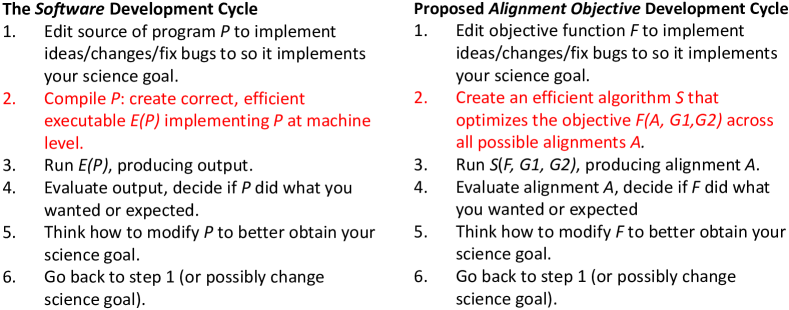
Figure 2: Comparison of the standard software development cycle (left), and proposed cycle for developing new objective functions for alignment (right). Red highlights the step that should be entirely automated and requiring no effort on the user’s part.

1.3.5 Using sequence similarity as an objective—a necessary but hopefully temporary evil

It may help here to (re-)state the obvious: the whole point of network alignment is to align networks based upon their network topology. This is a desirable goal because there is a strong belief that the topology of a network is somehow related to its function. For example, we believe that humans and chimpanzees are very close relatives, taxonomically speaking. If there is a particular protein $h_{0}$ in humans that performs a certain function by interacting with seven other proteins $h_{1},h_{2},\ldots,h_{7}$, then it is quite likely that there is a very similar protein $c_{0}$ in chimpanzees that also interacts with (close to) seven proteins $c_{1},c_{2},\ldots,c_{7}$ to perform virtually the same function. Another way of saying this is that the network topology of the protein-protein interaction networks of human and chimp are likely to be very similar in the vicinity of $h_{0}$ and $c_{0}$, respectively. As such, a natural network alignment between human and chimp should contain the ordered pairs $(h_{0},c_{0}),(h_{1},c_{1}),\ldots,(h_{7},c_{7})$. If the network of interactions around $h_{0}$ and $c_{0}$ are in fact similar, then any network alignment algorithm worth its mettle, optimizing an objective that highlights such network similarities, should include the above pairs with high likelihood.

The problem, at least in the research area of protein-protein interaciton (PPI) networks, is that the data on current PPI networks is extremely incomplete in terms of enumerating the edges in the PPI networks. For example, as of 2018, the most complete PPI network is that of S. cerevisiae, and it may be only about 50% complete; the human PPI network is probably less than 10% complete (Vidal, 2016); other species are even far less complete. For instance, we’d expect most mammals to have about the same number of interactions in their PPI networks, and yet the 2018 BioGRID Human network has almost 300,000 interactions, but mouse and rat have only 38,000 and 5,000 interactions listed, respectively. If Human is only 10% complete and currenthly contains 300,000 interactions, then we may expect the complete interactome to have over 1 million interactions. By this measure, mouse and rat are at most a few percent, and well less than one percent complete, respectively. Here’s the crux: if we are missing 90% or more of the edges in most mammal PPI networks, no network alignment algorithm based solely upon network topology has any hope of providing good alignments. This is the state of affairs in PPI network alignment.

Thus, it is no surprise that virtually every network alignment algorithm currently in existence must rely on using sequence similarity information to help give network alignments that show decent functional similarity. However, if network alignment is of any worth whatsoever, the use of sequence similarity should be viewed only as a temporary crutch—a necessary evil—until such time as the interactions in PPI networks are more completely enumerated.

On the other hand, since protein function is defined by the shape of the folded protein, and disrupting the function of a protein can be lethal, the folded structure of a protein tends to be better conserved than its sequence (Lesk and Chothia, 1986). This in turn suggests that the network of interactions may also be better conserved than sequence. If this is the case, then network alignment may ultimately be at least as useful as sequence alignment in terms of learning about protein function. Alas, we must wait until PPI networks are far more complete than they are today to test this hypothesis.

1.4 Search Algorithms

Given two networks with $n_{1}\leq n_{2}$ nodes, respectively, the number of possible 1-to-1 pairwise global network alignments between them is exactly $\frac{n_{2}!}{(n_{2}-n_{1})!}$. This is an enormous number; for example if the two networks each have thousands of nodes (not uncommon for protein-protein interaction networks), the the number of possible alignments can easily exceed $10^{100,000}$. This is an enormous search space, far larger, for example, than the number of elementary particles in the known universe—which according to Wikipedia is a paltry $10^{100}$.

The task of a network alignment algorithm is to search through this enormous space of possible alignments, looking for ones that score well according to one or more of the measures described in Section 1.2. Since network alignment is an NP-complete problem, all such algorithms must use heuristics to navigate this enormous search space. Search methods abound; several good review papers exist (Clark and Kalita, 2014; Faisal et al., 2015b; Milano et al., 2017; Guzzi and Milenković, 2017); for an extensive comparison specifically showing that SANA outperforms about a dozen of the best existing algorithms, see Mamano and Hayes (2017). SANA is virtually unique in that it was designed from the start to be able to optimize any objective function, including the objective functions introduced by other researchers; a preliminary report shows that SANA outperforms over a dozen other algorithms at optimizing their own objective functions (Kanne and Hayes, 2017).

1.5 Requirements of a good alignment algorithm

We believe that, in order to be of general use, a network alignment algorithm must satisfy the following properties:

Speed, if so desired.

SANA can produce better alignments in minutes that most other aligners can in hours. This is useful for many reasons: to perform test alignments; to experiment with objective functions; to perform multiple alignments of the same pair of networks in order to see which parts of the alignment, if any, come out the same each time (more on this later).

High quality of results, if so desired.

SANA’s primary user-tunable parameter is the amount of time the user wishes to wait. While SANA can produce better alignments in one minute on a laptop than many existing algorithms can do given hours of CPU, users can also tell SANA to spend any amount of time improving the alignment, such as 5 minutes, 3 hours, or a week. SANA generally produces better scoring alignments with longer run times, although we generally see a point of diminishing returns beyond a few hours.

It should be simple to use.

By this we mean that if there are any algorithmic parameters that crucially control the quality of the result, those parameters should be tuned automatically without user input—in other words, the user should not need be an expert on the algorithm in order to understand how to use it. The primary internal parameters controlling the anneal is the temperature schedule, and by default SANA spends a minute or two automatically finding a near-optimal temperature schedule before starting the anneal. (Another algorithm called SailMCS (Larsen et al., 2016) also uses simulated annealing but fails to automatically determine a good temperature schedule, and so SANA produces alignments that are far superior to those of SailMCS (Kanne and Hayes, 2017).)

Providing confidence estimates on the quality of the alignment.

For example, if some set of pegs $P_{1}$ always end up in the same holes every time SANA is run and another set of pegs $P_{2}$ end up in different holes each time SANA is run, this suggests the set $P_{1}$ is confidently aligned, whereas we should be suspicious about the alignment of pegs in $P_{2}$. Few algorithms are capable of this sort of confidence testing of the alignment; SANA, on the other hand, is so fast that it is easy to look for such core alignments (Milenković et al., 2010)—cf. Section 3.1.

Flexible with objective functions.

SANA has over a dozen pre-programmed objective functions that users can experiment with. In addition, users can supply SANA with externally computed similarity matrices, either node-to-node, or edge-to-edge. Finally, we have tried to make the code base of SANA clear so that anybody familiar with C++ can program new objective functions easily.

Able to handle nodes that have ASCII names rather than only allowing integers as node identifiers.

To a programmer, creating a mapping between ASCII names and integers is easy. To non-programmers this is not so easy, and many aligners have the inexcusable fault of insisting that nodes are named by sequential integers. SANA does this internally but allows users to use whatever names they want to identify nodes.

Available to plug in to existing popular tools such as Cytoscape.

SANA is available in the Cytoscape App store.

Able to handle multiple input graph formats.

Currently SANA only natively accepts networks in edge list format, and LEDA.gw format. The former is a line-by-line list of edges (two nodes from the same network listed on one line), while the latter is a rather deprecated format used by an old version of LEDA (Mehlhorn and Naher, 1999). However, we do provide a converter called createEdgeList that outputs our edge list format given any of the following input formats: GML, XML, graphML, LEDA, CSV, and LGF.

1.6 The value of randomness: core alignments

SANA shares one important aspect with a few other aligners including MAGNA (Saraph and Milenković, 2014; Vijayan et al., 2015) and OptNetAlign (Clark and Kalita, 2015): it is a randomized search algorithm. Like these other algorithms, SANA starts with a random alignment and then starts to move pegs around between holes; each time it tries to swap or move pegs around, it asks if the objective function has gotten better or not. As time progresses, the alignment gets better according to the objective function. If the objective function is an easy one to optimize, SANA will quickly find the optimal or near-optimal alignment (Mamano and Hayes, 2017; Kanne and Hayes, 2017); in harder cases it will simply find better-and-better solutions as it is given more time.

The fact that SANA intentionally injects randomness has some surprising positive aspects. In particular, if there exist highly similar regions between the two networks $G_{1}$ and $G_{2}$, SANA is likely to find them and align them identically every time, despite starting with a different random alignment each time. If there are other parts of the networks that are dissimilar and there is no obvious way to align them correctly, those regions are likely to get aligned differently each time SANA is run. Given two regions $R_{1}$ in $G_{1}$ and $R_{2}$ in $G_{2}$, the more topologically similar $R_{1}$ is to $R_{2}$, the more likely it is that SANA will align them the same way every time it is run, independent of the randomness. Since SANA is extremely fast, and since it has this random aspect, it is relatively painless to run SANA many times on the same pair of networks and look for pairs of nodes that are aligned together frequently. We use the term core alignment to refer to pairs of nodes that are stable across many runs of SANA; the more frequently a pair of nodes is aligned together, the more confident we are that they truly belong together according to the objective function being optimized. So for example, if we run SANA 10 times on the same 2 networks and produce output files out0.align, out1.align, out2.align, $\ldots$, out9.align, then we can trivially measure the core frequencies on the Unix command line as follows:

$ sort out?.align | uniq -c | sort -nr

The first sort puts identical lines from all 10 files side-by-side; the uniq -c counts how many unique lines are side-by-side (thus measuring core frequency), and the final sort -nr then sorts the aligned pairs of nodes by frequency, most frequent pairs of nodes first—that is, the most confident parts of the alignment are listed first. Note that the output of the above command line is a list of pairs precedid by their frequency. Note in particular that, even though SANA is a 1-to-1 aligner per run, with multiple runs we can produce non-1-to-1 mappings between the two networks, along with a confidence level for each particular pair.

1.7 Limitations of SANA

Currently, SANA aligns only two networks at a time. Each time, it produces a 1-to-1 mapping between the nodes of the smaller network to the nodes of the larger one (ie., an arrangement of pegs into holes). So technically, SANA is a global, pairwise, 1-to-1 alignment algorithm—the simplest type of global alignment algorithm. However, as we described above, SANA produces good alignments so quickly that it can be run many times on the same pair of networks in the same time it takes to run most other algorithms just once; by running SANA many times we effectively produce not only a non-1-to-1 mapping, but also a confidence estimate of each pair of nodes we output. So far as we are aware, no other algorithm produces such confidence estimates.

Furthermore, even though SANA technically aligns only 2 networks at a time, in the Appendix of this paper we describe a prototype version of multi-SANA that uses pairwise alignments to construct a multiple network alignment.

Thus, although SANA is technically only a 1-to-1 pairwise network aligner, it can effectively produce both many-to-many alignments (with confidences), and multiple alignments.

2 Examples of usage

2.1 Getting started with SANA

# Lines like this are comments. The Unix/Bash prompt is the dollar sign.
# First use "git" to clone the repo:
$ git clone http://github.com/waynebhayes/SANA
Cloning into ’SANA’... #git output deleted
$ cd SANA; make   # now wait a few minutes...
# Run SANA for the first time on the 2018 BioGRID networks of rat and S. pombe:
$ ./sana -fg1 networks/RNorvegicus18.el -fg2 networks/SPombe18.el
# wait while SANA computes a temperature schedule and then performs the alignment...
$ cat sana.out # look at the output file; first line is an internal
# representation of the alignment and can be ignored.
$ head -3 sana.align # left column is a BioGRID node name from rat, right from S.pombe.
361207  2542195
316265  2541287
499382  2539901
$

Table 1: Getting started with SANA on the Unix command line. We first clone the repo from GitHub, then “make” SANA, then run it on the two smallest BioGRID 2018 networks: R. norvegicus and S. pombe. We then look at the output file sana.out, which contains scores and other useful information, as well as the actual alignment file sana.align. SANA has many command-line options; type “../sana -h | less” to see a long list of them.

Table 1 contains a sequence of Unix Shell commands that will download the repo from GitHub, compile SANA, and perform your first test of SANA to ensure everything works.

The most basic run of SANA requires the user only to specify which two networks to align; in Table 1 it is the 2018 BioGRID renditions of Rattus norvegicus (the common sewer rat, aka lab rat), and the single-celled yeast Schizosaccharomyces pombe. SANA defaults to using $S^{3}$ as the objective function, and 5 minutes as the amount of time to perform simulated annealing. Total run time is about 6–7 minutes including the initial computation of the temperature schedule, which we now describe.

Simulated annealing only works well if the temperature schedule is chosen carefully. We must start with a temperature high enough that moves are essentially random, so that even bad moves are frequently accepted (this keeps us out of local minima); and then end with a temperature low enough that only good moves are accepted (to hone in on the best local maximum once we’ve found its general vicinity). Empirically, we are controlling the probability of accepting a bad move, or pBad; it must start close to 1, and end close to zero. Unfortunately there’s no analytical method to compute these extremes, so the first 1-2 minutes of SANA are spent estimating the initial temperature $t_{initial}$, the final temperature $t_{final}$ that gives a pBad starting near 1 and ending near zero, along with the $t_{decay}$, the temperature decay rate that gets us from one to the other in the allotted time (5 minutes by default).

Next you will see the statement, Start execution of SANA_s3 which says SANA is finally starting the anneal, optimizing s3. After that, you’ll see updates every few seconds as SANA progresses. These updates show the update number, the elapsed time so far, the current score, some statistical theoretical values that don’t concern us here, and the sampled pBad, which should start above 0.98 and end somewhere below about 1e-6.

Once SANA is finished running, there are exactly two output files (whose names can be changed with the “-o” option): sana.out contains as its first (long) line an internal representation of the alignment, followed by some human-readable statistics; an example is in Table 2. The second file, called sana.align, contains the actual alignment in two-column format: on each line, the left column contains a node (“peg”) from $G_{1}$ and the right column is the aligned node (“hole”) from $G_{2}$.

Table 2: The sana.out file (whose name can be changed using the -o command-line option) contains information about the input networks (nodes, edges, connected components) and an analysis of the alignment (various measures applied to the entire alignment, and also applied to the common connected subgraphs).

2018-06-15 15:21:57

G1: yeast
n    = 2390
m    = 16127
#connectedComponents = 158
Largest connectedComponents (nodes, edges) = (1994, 15819) (10, 32) (6, 11)

G2: human
n    = 9141
m    = 41456
#connectedComponents = 94
Largest connectedComponents (nodes, edges) = (8934, 41341) (5, 4) (4, 3)

Method: SANA_s3
Temperature schedule:
T_initial: 0.000316228
T_decay: 6.61993
Optimize:
weight s3: 1
Requested Execution time: 5 minutes

Actual execution time = 300.976 seconds

Random Seed: 514154230

Scores:
ec: 0.397966
mec: 1
ses: 35381
ics: 0.831563
s3: 0.368279
lccs: 0.248768
sec: 0.222913

Common subgraph:
n    = 2390
m    = 6418
#connectedComponents = 395
Largest connectedComponents (nodes, edges) = (1059, 4805) (53, 263) (48, 69)

Common connected subgraphs:
Graph  n     m      alig-edges  indu-edges  EC        ICS       S3
G1     2390  16127  6418        7718        0.397966  0.831563  0.368279
CCS_0  1059  4805   4805        5790        1.000000  0.829879  0.829879
CCS_1  53    263    263         268         1.000000  0.981343  0.981343
CCS_2  48    69     69          73          1.000000  0.945205  0.945205
CCS_3  34    68     68          70          1.000000  0.971429  0.971429
CCS_4  33    50     50          52          1.000000  0.961538  0.961538

The default objective function is $S^{3}$; changing the objective function is easy on the command line. For example to have SANA optimize a 50-50 combination of $EC$ and $S^{3}$, type

./sana -ec 0.5 -s3 0.5 -fg1 ...

To turn off $S^{3}$ entirely and perform an $EC$-only alignment, do

./sana -s3 0 -ec 1 -fg1 ...

To perform an alignmet that optimizes 90% Importance as defined by HubAlign (Hashemifar and Xu, 2014) 5% graphlets as used by GRAAL (Kuchaiev et al., 2010), 5% EC, and no $S^{3}$, do

./sana -s3 0 -importance 0.9 -graphlets 0.05 -ec 0.05 ...

Note that one does not need to manually ensure that all the weights specified on the command line add to 1; if they do not, SANA will simply re-normalize them all so that they add to 1.

Similarly, the are many other objective functions defined by SANA; currently implemented ones are listed in Table 3.

2.2 Direct comparison with other aligners

As a part of our first publication on SANA (Mamano and Hayes, 2017), we wanted to automate the process of directly comparing to many other existing aligners. Thus, the external source code of over a dozen existing aligners were directly incorporated into SANA so that they can be called from the SANA command line. This was done to ensure consistent calling conventions to these other aligners during our comparisons. These other methods can be called from the SANA command line using the -method argument. In the SANA repo, these other aligners are in the directory wrappedAlgorithms; see the online SANA documentation for more details. The other aligners currently incorporated into SANA are LGRAAL (Malod-Dognin and Pržulj, 2015), MAGNA++ (Vijayan et al., 2015), HubAlign (Hashemifar and Xu, 2014), WAVE (Sun et al., 2015), NETAL (Neyshabur et al., 2013), MIGRAAL (Kuchaiev and Pržulj, 2011), GHOST (Patro and Kingsford, 2012), PISWAP (Chindelevitch et al., 2013), OptNetAlign (Clark and Kalita, 2015), SPINAL (Aladağ and Erten, 2013), GREAT (Crawford and Milenković, 2015), NATALIE 2.0 (El-Kebir et al., 2011), GEDEVO (Ibragimov et al., 2013), CytoGEDEVO (Malek et al., 2016), BEAMS (Alkan and Erten, 2014), HGRAAL (Milenković et al., 2010), PINALOG (Phan and Sternberg, 2012).

Table 3: Measures accepted by SANA on the command line. Note that “Name” means “command-line option”, so for example to give ec a weight of 0.5, use “-ec 0.5” on the SANA command line.

Name	Description
s3	Symmetric Substructure Score (Saraph and Milenković, 2014)
ec	Edge Coverage/Correspondence/Correctness (Kuchaiev et al., 2010)
ics	Induced Conserved Structure (Patro and Kingsford, 2012)
graphlet	Orbit Degree Vector (ODV) Similarity (Milenković and Pržulj, 2008; Kuchaiev et al., 2010)
graphletlgraal	LGRAAL-normalization of ODV sim (Malod-Dognin and Pržulj, 2015)
go	Mean ResnikMax GO similarity (Resnik, 1995; Ashburner et al., 2000)
NetGO	Network-alignment-based GO similarity (Hayes and Mamano, 2017)
wec	Weighted EC (Sun et al., 2015)
esim	External file defining node-pair similarities
sequence	BLANT-based sequence similarities (Camacho et al., 2009)
lccs	Largest Common Connected Subgraph (Kuchaiev et al., 2010)
nc	Node Correctness (if known, defines the exact alignment)
spc	Shortest Path Conservation (Mamano and Hayes, 2017)
edgeCount	degree difference
edgeDensity	relative degree difference
importance	HubAlign’s Importance (Hashemifar and Xu, 2014)
nodeDensity	local node density
ewec	External edge-based similarity matrix, eg., edge-graphlet similarity(Crawford and Milenković, 2015)
sequence	BLAST bit scores based on protein sequence similarity (Camacho et al., 2009)

3 An example of objective function experimentation

As shown in Figure 2, SANA can be used to experiment with objective functions; we believe that such experimentation is one of the most important but apparently under-appreciated aspects of the science of network alignment. Here we describe one such experiment with a very well-defined scientific goal.

3.1 Gene–microRNA networks

Table 4: Table of results when testing various objective functions (leftmost column) for their ability to correctly align genes-to-genes, and mRNAs-to-mRNAs, when aligning a pair of gene-mNRA networks (Tokar et al., 2017). Objectives tested were $EC$ (Kuchaiev et al., 2010), $S^{3}$ (Saraph and Milenković, 2014), Importance (Hashemifar and Xu, 2014), graphlet (Milenković and Pržulj, 2008; Kuchaiev et al., 2010), and graphlet-LGRAAL (Malod-Dognin and Pržulj, 2015). The columns are as follows. pairs: total number of pairs of nodes aligned in all 1,000 network pairs that were run 5 times each. 2*Gene: number of pairs in which a gene was correctly aligned to another gene. mix: number of pairs in which a gene in one network was aligned to an mRNA in the other. 2*RNA: number of pairs in which an mRNA was aligned to another mRNA. coreFreq(XY)$>1$: the number of aligned pairs that had a core frequency greater than 1 (indicating the objective function strongly prefers to align this pair of nodes together) for type-pairs GG, MG, and MM.

1 minute runs
objective	pairs	2*Gene	mix	2*RNA	coreFreq(GG)$>1$	coreFreq(MG)$>1$	coreFreq(MM)$>1$
ec	30424880	29953074	198792	273014	1268806	570	3169
s3	30424880	29986047	284470	154363	1093307	2947	688
importance	30241594	25434876	4658345	148373	651969	114137	1386
graphlet-GRAAL	30424880	24109670	6176510	138700	1902554	449738	17331
graphlet-LGRAAL	30424880	23056815	7305611	62454	1718519	584735	7086
4 minute runs
objective	pairs	2*Gene	mix	2*RNA	coreFreq(GG)$>1$	coreFreq(MG)$>1$	coreFreq(MM)$>1$
ec	30424880	30055465	97811	271604	1245103	208	5908
s3	30424880	29953309	283313	188258	1092319	3779	1508
importance	30292547	25473995	4669942	148610	652830	114815	1621
graphlet-GRAAL	30424880	24104880	6180836	139164	2208583	502806	25308
graphlet-LGRAAL	30424880	23051615	7310109	63156	2090416	692752	10504

Consider a set of gene-microRNA (mRNA) networks (Tokar et al., 2017), one network for each species. These networks are bipartite, meaning that genes interact with microRNAs, but neither genes nor microRNAs interact with their own type. Thus, when aligning two gene-mRNA networks, we wish to align genes from one network to genes in the other, and mRNAs in one to mRNAs in the other, but we should never align a gene to an mRNA or vice-versa. In essence, the nodes have two types, and we must provide a type-specific network alignment.

At first, SANA did not have the functionality to provide a typed-node alignment. The question was: how do the various topological objective functions compare in their ability to automatically align types correctly, given that typing is not enforced by the alignment algorithm?

Referring to Figure 2, the scientific goal is clear: maximize the fraction of nodes that are aligned to like-type nodes in the other network. The question is now, which topological objective function best achieves this scientific goal?

We received 535 networks directly from one of the authors of Tokar et al. (2017). We chose 1,000 pairs of networks at random out of the ${535\choose 2}=142,845$ possible pairs of networks. For each pair of networks, we tested the following objective functions for their ability to correctly align nodes of like type to each other when this was not enforced: $EC$, $S^{3}$, Importance (Hashemifar and Xu, 2014), GRAAL-type graphlet orbit signatures (Milenković and Pržulj, 2008; Kuchaiev et al., 2010), and LGRAAL-type graphlet orbit signatures (Malod-Dognin and Pržulj, 2015). To further test the dependence on runtime, we ran SANA on all the above objectives for all 1,000 networks for runtimes of 1 and 4 minutes. Finally, to look at the frequency of core alignments, we performed each of the above pairs 5 times each. The results are in Table 4.

One column of great interest is the “mix” column, which counts the number of times, out of the approximately 30 million pairs of aligned nodes, in which a gene from one network was aligned to an mRNA in the other network—which is the kind of mis-typed node alignment we are trying to avoid. The rows are sorted best-to-worst by this measure, in each of the 1-minute and 4-minute sub-tables. As we can see, the $EC$ objective scores best at avoiding this kind of mis-typed alignment. In the 1-minute runs, $EC$ aligns unlike typed node-pairs in only 0.65% of cases; $S^{3}$ is a close second, mis-typing just under 1% of the aligned pairs of nodes. In contrast, HubAlign’s Importance measure (Hashemifar and Xu, 2014) is almost 20 times worse in terms of incorrectly aligning nodes of different types, doing so in about 15% of aligned pairs of nodes, while both graphlet measures fare the worst, aligning unlike-type nodes in over 20% of cases.

Even more interesting is the 4 minute runs, in which $EC$ cuts its mis-typed node alignment in half, down to about 0.3% of aligned pairs, while all other measures fail to improve their “mix” column with the longer runtime.

Recall that if SANA aligns the same pair of nodes together in more than one run, we say that pair is in the core alignment, because the objective function is unlikely to align two nodes together more than once by chance. Another column of great interest is thus the coreFreq(MG)$>1$ column, which tells us how frequently the objective function seems to strongly prefer mis-aligning a pair of nodes of different types. Again we see that the $EC$ measure is by far the best measure by this criterion: in the 1 minute runs, only 570 mistyped pairs appear out of 30 million (about 2 per 100,000 pairs), while the 4 minute runs cut that “error rate” in half, suggesting that longer runs will do a better job of correctly aligning types. Meanwhile, $S^{3}$ does 10x worse at 1 minute and gets more bad in the 4 minute runs, while importance and both graphlet measures misalign orders of magnitude more typed pairs, presenting a strong preference for misaligning nodes in about 1–2% of pairs.

We conclude that the $EC$ measure is, by far, the best available objective function for this particular purpose among those we tested. For the moment we do not hypothesize why this is the case, but empirically the result seems iron-clad. While we agree that the $S^{3}$ measure is mathematically more aesthetically pleasing and would seem to be a better measure intuitively, for this particular purpose $EC$ seems to work better. The author finds the poor performance of graphlet-based measures particularly surprising, since the author is a strong believer that graphlets are a useful tool for network analysis (see for example Hasan et al. (2017))—and graphlets have certainly demonstrated their value in other contexts (Davis et al., 2015; Yaveroğlu et al., 2014). However, these results suggest that perhaps orbit degree signatures as they are currently defined (Milenković and Pržulj, 2008; Kuchaiev et al., 2010; Malod-Dognin and Pržulj, 2015) may not be the best way to leverage graphlet-based information in the context of global pairwise network alignment.

4 Conclusion

We have described the use of SANA (Mamano and Hayes, 2017), the Simulated Annealing Network Aligner, in the context of the pairwise 1-to-1 global alignment of biological networks. SANA provides many advantages over the many other aligners currently available: as a search algorithm, it is lightning fast, producing well-scoring alignments in minutes rather than hours; it provides a large array of objective functions users may wish to experiment with, as well as the facility to add more objectives in the future; it does not require the user to know much about the internal workings of the aligner in order to use it; and it is well on the way towards being fully integrated into popular network analysis tools such as Cytoscape.

We have introduced the concept of objective function experimentation (cf. Figure 2 and Section 3.1), which we believe is at the core of future developments in network alignment. SANA’s speed and effectiveness makes it the ideal aligner to implement the process depicted in Figure 2.

Appendix

A prototype of a multiple-network-alignment version of SANA is available in the SANA GitHub repo. Simply re-compile SANA with the -DWEIGHTED option on the command line (see the Makefile), and the consult the Bourne shell script multi-pairwise.sh; running it without any arguments provides a short help message.

Questions about SANA, comments, or feature requests should be directed to the author at whayes@uci.edu.

References

- Aladağ and Erten (2013) Aladağ, A. E. and Erten, C. (2013). Spinal: scalable protein interaction network alignment. Bioinformatics, 29(7), 917–924.
- Alkan and Erten (2014) Alkan, F. and Erten, C. (2014). Beams: backbone extraction and merge strategy for the global many-to-many alignment of multiple ppi networks. Bioinformatics, 30(4), 531–539.
- Ashburner et al. (2000) Ashburner, M., Ball, C. A., Blake, J. A., Botstein, D., Butler, H., Cherry, J. M., Davis, A. P., Dolinski, K., Dwight, S. S., Eppig, J. T., Harris, M. A., Hill, D. P., Issel-Tarver, L., Kasarskis, A., Lewis, S., Matese, J. C., Richardson, J. E., Ringwald, M., Rubin, G. M., and Sherlock, G. (2000). Gene Ontology: tool for the unification of biology. Nature Genetics, 25(1), 25–29.
- Camacho et al. (2009) Camacho, C., Coulouris, G., Avagyan, V., Ma, N., Papadopoulos, J. S., Bealer, K., and Madden, T. L. (2009). Blast+: architecture and applications. BMC Bioinformatics, 10, 421.
- Chatr-Aryamontri et al. (2017) Chatr-Aryamontri, A., Oughtred, R., Boucher, L., Rust, J., Chang, C., Kolas, N. K., O’Donnell, L., Oster, S., Theesfeld, C., Sellam, A., et al. (2017). The biogrid interaction database: 2017 update. Nucleic acids research, 45(D1), D369–D379.
- Chen and Rajewsky (2007) Chen, K. and Rajewsky, N. (2007). The evolution of gene regulation by transcription factors and micrornas. Nature reviews. Genetics, 8(2), 93.
- Chindelevitch et al. (2013) Chindelevitch, L., Ma, C.-Y., Liao, C.-S., and Berger, B. (2013). Optimizing a global alignment of protein interaction networks. Bioinformatics, 29(21), 2765–2773.
- Clark and Kalita (2014) Clark, C. and Kalita, J. (2014). A comparison of algorithms for the pairwise alignment of biological networks. Bioinformatics, 30(16), 2351–2359.
- Clark and Kalita (2015) Clark, C. and Kalita, J. (2015). A multiobjective memetic algorithm for ppi network alignment. Bioinformatics, 31(12), 1988–1998.
- Consortium (2008) Consortium, T. G. O. (2008). The gene ontology project in 2008. Nucleic Acids Research, 36(suppl 1), D440–D444.
- Cook (1971) Cook, S. A. (1971). The complexity of theorem-proving procedures. In Proceedings of the third annual ACM symposium on Theory of computing, pages 151–158. ACM.
- Crawford and Milenković (2015) Crawford, J. and Milenković, T. (2015). Great: graphlet edge-based network alignment. In Bioinformatics and Biomedicine (BIBM), 2015 IEEE International Conference on, pages 220–227. IEEE.
- Davidson (2010) Davidson, E. H. (2010). The regulatory genome: gene regulatory networks in development and evolution. Academic press, USA.
- Davis et al. (2015) Davis, D., Yaveroğlu, Ö. N., Malod-Dognin, N., Stojmirovic, A., and Pržulj, N. (2015). Topology-function conservation in protein–protein interaction networks. Bioinformatics, 31(10), 1632–1639.
- El-Kebir et al. (2011) El-Kebir, M., Heringa, J., and Klau, G. W. (2011). Lagrangian relaxation applied to sparse global network alignment. In IAPR International Conference on Pattern Recognition in Bioinformatics, pages 225–236. Springer.
- Faisal et al. (2015a) Faisal, F. E., Meng, L., Crawford, J., and Milenković, T. (2015a). The post-genomic era of biological network alignment. EURASIP Journal on Bioinformatics and Systems Biology, 2015(1), 3.
- Faisal et al. (2015b) Faisal, F. E., Meng, L., Crawford, J., and Milenković, T. (2015b). The post-genomic era of biological network alignment. EURASIP Journal on Bioinformatics and Systems Biology, 2015(1), 1.
- Farazi et al. (2013) Farazi, T. A., Hoell, J. I., Morozov, P., and Tuschl, T. (2013). Micrornas in human cancer. In MicroRNA Cancer Regulation, pages 1–20. Springer, Germany.
- Fiehn (2002) Fiehn, O. (2002). Metabolomics-the link between genotypes and phenotypes. In Functional Genomics, pages 155–171. Springer, Germany.
- Garey and Johnson (1979) Garey, M. and Johnson, D. (1979). Computers and Intractability: A Guide to the Theory of NP-Completeness. New York: W.H. Freeman, New York.
- Guzzi and Milenković (2017) Guzzi, P. H. and Milenković, T. (2017). Survey of local and global biological network alignment: the need to reconcile the two sides of the same coin. Briefings in bioinformatics, page bbw132.
- Hasan et al. (2017) Hasan, A., Chung, P.-C., and Hayes, W. (2017). Graphettes: Constant-time determination of graphlet and orbit identity including (possibly disconnected) graphlets up to size 8. PloS one, 12(8), e0181570.
- Hashemifar and Xu (2014) Hashemifar, S. and Xu, J. (2014). HubAlign: an accurate and efficient method for global alignment of protein–protein interaction networks. Bioinformatics, 30(17), i438–i444.
- Hayes and Mamano (2017) Hayes, W. B. and Mamano, N. (2017). Sana netgo: a combinatorial approach to using gene ontology (go) terms to score network alignments. Bioinformatics, 34(8), 1345–1352.
- Hočevar and Demšar (2014) Hočevar, T. and Demšar, J. (2014). A combinatorial approach to graphlet counting. Bioinformatics, 30(4), 559–565.
- Ibragimov et al. (2013) Ibragimov, R., Malek, M., Guo, J., and Baumbach, J. (2013). Gedevo: an evolutionary graph edit distance algorithm for biological network alignment. In OASIcs-OpenAccess Series in Informatics, volume 34. Schloss Dagstuhl-Leibniz-Zentrum fuer Informatik.
- Jaenicke and Helmreich (2012) Jaenicke, R. and Helmreich, E. (2012). Protein-protein interactions, volume 23. Springer Science & Business Media, Germany.
- Junker and Schreiber (2011) Junker, B. H. and Schreiber, F. (2011). Analysis of biological networks, volume 2. John Wiley & Sons, USA.
- Kanne and Hayes (2017) Kanne, D. P. and Hayes, W. B. (2017). Sana: separating the search algorithm from the objective function in biological network alignment, part 1: Search.
- Karlebach and Shamir (2008) Karlebach, G. and Shamir, R. (2008). Modelling and analysis of gene regulatory networks. Nature reviews. Molecular cell biology, 9(10), 770.
- Kotlyar et al. (2015) Kotlyar, M., Pastrello, C., Sheahan, N., and Jurisica, I. (2015). Integrated interactions database: tissue-specific view of the human and model organism interactomes. Nucleic acids research, 44(D1), D536–D541.
- Kuchaiev and Pržulj (2011) Kuchaiev, O. and Pržulj, N. (2011). Integrative network alignment reveals large regions of global network similarity in yeast and human. BIOINFORMATICS, 27, 1390–1396.
- Kuchaiev et al. (2010) Kuchaiev, O., Milenković, T., Memišević, V., Hayes, W., and Pržulj, N. (2010). Topological network alignment uncovers biological function and phylogeny. Journal of The Royal Society Interface, 7(50), 1341–1354.
- Larsen et al. (2016) Larsen, S. J., Alkærsig, F. G., Ditzel, H. J., Jurisica, I., Alcaraz, N., and Baumbach, J. (2016). A simulated annealing algorithm for maximum common edge subgraph detection in biological networks. In Proceedings of the 2016 on Genetic and Evolutionary Computation Conference, pages 341–348. ACM.
- Lesk and Chothia (1986) Lesk, A. and Chothia, C. (1986). The response of protein structures to amino-acid sequence changes. Phil. Trans. R. Soc. Lond. A, 317(1540), 345–356.
- Malek et al. (2016) Malek, M., Ibragimov, R., Albrecht, M., and Baumbach, J. (2016). Cytogedevo—global alignment of biological networks with cytoscape. Bioinformatics, 32(8), 1259–1261.
- Malod-Dognin and Pržulj (2015) Malod-Dognin, N. and Pržulj, N. (2015). L-graal: Lagrangian graphlet-based network aligner. Bioinformatics.
- Mamano and Hayes (2017) Mamano, N. and Hayes, W. B. (2017). Sana: Simulated annealing far outperforms many other search algorithms for biological network alignment. Bioinformatics (Oxford, England), 33, 2156–2164.
- Mehlhorn and Naher (1999) Mehlhorn, K. and Naher, S. (1999). Leda: A platform for combinatorial and geometric computing. Cambridge University Press, United Kingdom.
- Milano et al. (2017) Milano, M., Guzzi, P. H., Tymofieva, O., Xu, D., Hess, C., Veltri, P., and Cannataro, M. (2017). An extensive assessment of network alignment algorithms for comparison of brain connectomes. BMC bioinformatics, 18(6), 235.
- Milenković and Pržulj (2008) Milenković, T. and Pržulj, N. (2008). Uncovering biological network function via graphlet degree signatures. Cancer Inform., 6(Epub 2008 Apr 14), 257–273.
- Milenković et al. (2010) Milenković, T., Ng, W. L., Hayes, W., and Pržulj, N. (2010). Optimal network alignment with graphlet degree vectors. Cancer Informatics, 9, 121–137.
- Neyshabur et al. (2013) Neyshabur, B., Khadem, A., Hashemifar, S., and Arab, S. S. (2013). Netal: a new graph-based method for global alignment of protein–protein interaction networks. Bioinformatics, 29(13), 1654–1662.
- Patro and Kingsford (2012) Patro, R. and Kingsford, C. (2012). Global network alignment using multiscale spectral signatures. Bioinformatics, 28(23), 3105–3114.
- Phan and Sternberg (2012) Phan, H. T. and Sternberg, M. J. (2012). Pinalog: a novel approach to align protein interaction networks—implications for complex detection and function prediction. Bioinformatics, 28(9), 1239–1245.
- Prescott (2012) Prescott, D. M. (2012). Cell Biology A Comprehensive Treatise V3: Gene Expression: The Production of RNA’s, volume 3. Elsevier, Amsterdam-London-New York-Oxford-Paris-Shannon-Tokyo.
- Pržulj et al. (2004a) Pržulj, N., Wigle, D., and Jurisica, I. (2004a). Functional topology in a network of protein interactions. Bioinformatics, 20(3), 340–348.
- Pržulj et al. (2004b) Pržulj, N., Corneil, D. G., and Jurisica, I. (2004b). Modeling interactome: scale-free or geometric? Bioinformatics, 20(18), 3508–3515.
- Resnik (1995) Resnik, P. (1995). Using information content to evaluate semantic similarity in a taxonomy. arXiv preprint cmp-lg/9511007.
- Rossi et al. (2017) Rossi, R. A., Zhou, R., and Ahmed, N. K. (2017). Estimation of graphlet statistics. arXiv preprint arXiv:1701.01772.
- Saraph and Milenković (2014) Saraph, V. and Milenković, T. (2014). MAGNA: maximizing accuracy in global network alignment. Bioinformatics, 30(20), 2931–2940.
- Sporns (2010) Sporns, O. (2010). Networks of the Brain. MIT press, USA.
- Sun et al. (2015) Sun, Y., Crawford, J., Tang, J., and Milenkovic̀, T. (2015). Simultaneous optimization of both node and edge conservation in network alignment via WAVE. In M. Pop and H. Touzet, editors, Algorithms in Bioinformatics, volume 9289 of Lecture Notes in Computer Science, pages 16–39. Springer Berlin Heidelberg, Germany.
- Tokar et al. (2017) Tokar, T., Pastrello, C., Rossos, A. E., Abovsky, M., Hauschild, A.-C., Tsay, M., Lu, R., and Jurisica, I. (2017). mirdip 4.1—integrative database of human microrna target predictions. Nucleic acids research, 46(D1), D360–D370.
- Van El et al. (2013) Van El, C. G., Cornel, M. C., Borry, P., Hastings, R. J., Fellmann, F., Hodgson, S. V., Howard, H. C., Cambon-Thomsen, A., Knoppers, B. M., Meijers-Heijboer, H., et al. (2013). Whole-genome sequencing in health care: recommendations of the european society of human genetics. European Journal of Human Genetics, 21(6), 580.
- Vidal (2016) Vidal, M. (2016). How much of the human protein interactome remains to be mapped?
- Vijayan and Milenković (2017) Vijayan, V. and Milenković, T. (2017). Aligning dynamic networks with dynawave. Bioinformatics, 34(10), 1795–1798.
- Vijayan et al. (2015) Vijayan, V., Saraph, V., and Milenković, T. (2015). Magna++: Maximizing accuracy in global network alignment via both node and edge conservation. Bioinformatics, 31(14), 2409–2411.
- Von Mering et al. (2002) Von Mering, C., Krause, R., Snel, B., Cornell, M., et al. (2002). Comparative assessment of large-scale data sets of protein-protein interactions. Nature, 417(6887), 399.
- Williamson and Sutcliffe (2010) Williamson, M. P. and Sutcliffe, M. J. (2010). Protein–protein interactions.
- Yang et al. (2018) Yang, C., Lyu, M., Li, Y., Zhao, Q., and Xu, Y. (2018). Ssrw: A scalable algorithm for estimating graphlet statistics based on random walk. In International Conference on Database Systems for Advanced Applications, pages 272–288. Springer.
- Yaveroğlu et al. (2014) Yaveroğlu, Ö. N., Malod-Dognin, N., Davis, D., Levnajic, Z., Janjic, V., Karapandza, R., Stojmirovic, A., and Pržulj, N. (2014). Revealing the hidden language of complex networks. Scientific reports, 4, 4547.