Constructing Minimal Perfect Hash Functions Using SAT Technology

Abstract

Minimal perfect hash functions (MPHFs) are used to provide efficient access to values of large dictionaries (sets of key-value pairs). Discovering new algorithms for building MPHFs is an area of active research, especially from the perspective of storage efficiency. The information-theoretic limit for MPHFs is $\frac{1}{\ln 2}\approx 1.44$ bits per key. The current best practical algorithms range between 2 and 4 bits per key. In this article, we propose two SAT-based constructions of MPHFs. Our first construction yields MPHFs near the information-theoretic limit. For this construction, current state-of-the-art SAT solvers can handle instances where the dictionaries contain up to 40 elements, thereby outperforming the existing (brute-force) methods. Our second construction uses XORSAT filters to realize a practical approach with long-term storage of approximately $1.83$ bits per key.

Introduction

A minimal perfect hash function (MPHF) for a set $Y$ with $n$ distinct elements is a collision-free mapping from the elements of $Y$ to the set $[n]=\{1,\dots,n\}$. MPHFs enable efficient access to data stored in large databases by providing a unique index for each key in a set of key-value pairs. This allows the value of each key-value pair to be stored at its associated index in an $n$-entry table. Since industrial databases are often of significant size, if an MPHF is going to be used, one would want it to use as little extra space as possible.

The information-theoretic limit for MPHFs is $\frac{1}{\ln 2}\approx 1.44$ bits per key (?; ?), yet no practical constructions (those not relying on brute-force) have been found that meet this limit. In fact, the current best algorithms range between 2 and 4 bits per key (?; ?; ?; ?). Since applications may also consider costs such as build time and query time, MPHF construction and querying should not be so costly as to outweigh the benefit of a compact representation.

We introduce two new constructions for static MPHFs: i.e., MPHFs where the set $Y$ is immutable and known in advance. Both constructions are based on satisfiability (SAT) techniques and utilize a universal family of hash functions.

Our first construction encodes the MPHF construction as a Boolean formula and computes a solution for it using a SAT solver. It aims at the construction of MPHFs near the information-theoretic limit (roughly $1.44$ bits per key for large sets, say consisting of over a few thousand keys) and can be queried in $\log_{2}n$ steps. The information-theoretic limit $\alpha_{n}$ for smaller values of $n$ are shown in Table 1.

We present a compact $\mathcal{O}(n^{2}\log_{2}n)$ SAT encoding and a more effective $\mathcal{O}(n^{3})$ encoding. On these encodings, current SAT solvers (both complete and incomplete approaches) exhibit exponential runtime on the number of elements in the dictionary, with runtimes growing prohibitively large around $40$ elements, making our construction currently impractical for large sets. However, to the best of our knowledge, no other existing construction (including brute-force) can construct MPHFs near the information-theoretic limit for sets with more than $20$ elements in reasonable time.

Since we are only interested in satisfiable formulas (existence of MPHFs), SAT approaches based on local-search technology seem a natural fit. Currently complete solving methods work best on our encodings. However, our construction creates formulas with a strong random flavor and enormous progress has been made on local-search techniques for uniform random $k$-SAT instances (?; ?; ?).

Our second construction uses approximately $1.83$ bits per key and can build MPHFs in $\mathcal{O}(n^{3})$ steps (though construction is trivially parallelizable). These MPHFs can be queried in $max(3,\ln n+\ln(\ln n))$ steps in the worst case. Formally, the construction involves storing a minimum-weight perfect matching of a weighted bipartite graph in a space-efficient retrieval structure called an XORSAT filter (?). Our implemented prototype demonstrates that the approach can produce MPHFs for large datasets ($2^{30}$ keys) with fast query speed (a million queries per second) for low costs.

Table 1: The information-theoretic limit ($\alpha_{n}$) of bits per key for a various number of keys ($n$).

$n$	$10$	$20$	$30$	$40$	$10^{2}$	$10^{3}$	$10^{4}$
$\alpha_{n}$	$1.143$	$1.268$	$1.317$	$1.343$	$1.396$	$1.436$	$1.442$

Preliminaries

Below we present the most important background concepts related to the contributions of this paper.

Minimal Perfect Hash Functions.

A minimal perfect hash function (MPHF) for a set $Y$ with $n$ distinct elements is a bijection that maps the elements from $Y$ to the set $[n]=\{1,...,n\}$. Three important tradeoffs play a role when constructing MPHFs: storage space, query speed, and building cost. Most research focuses on lowering the storage space, while having acceptable query speed and building cost.

The probability that a universal function $H$ with range $[n]$ is a minimal perfect hash function for $Y$ is $\frac{n!}{n^{n}}$. For each element $y_{i}$ with $i\in[n]$, the probability that $H(y_{i})$ and $H(y_{j})$ with $(j<i)$ don’t collide is $\frac{n+1-i}{n}$. The information theoretic limit $\alpha_{n}$ is ${\log_{2}(\frac{n^{n}}{n!})}/n$ bits per element. This limit is roughly $1.44$ bits per element for large $n$, but smaller for small $n$. Table 1 shows the limit for various values of $n$.

The only existing MPHF constructions that realize this bound are based on brute-force: they evaluate many hash functions on $Y$ and terminate as soon as a minimal perfect hash function is found. As the representation of such a hash function requires on average $\alpha_{n}$ bits per element, it follows that, for example, brute-force over a set of $20$ elements requires on average evaluating over 43 million ($2^{25.36}$) hash functions.

Propositional Logic and Satisfiability.

We consider propositional formulas in conjunctive normal form, which are defined as follows. A literal is either a variable $x$ (a positive literal) or the negation $\overline{x}$ of a variable $x$ (a negative literal). For a literal $l$, we denote the variable of $l$ by $\mathit{var}(l)$. The complementary literal $\overline{l}$ of a literal $l$ is defined as $\overline{l}=\overline{x}$ if $l=x$ and $\overline{l}=x$ if $l=\overline{x}$. A clause is a finite disjunction of the form $(l_{1}\lor\dots\lor l_{k})$, where $l_{1},\dots,l_{k}$ are literals. A formula is a finite conjunction of the form $C_{1}\land\dots\land C_{m}$, where $C_{1},\dots,C_{m}$ are clauses. An XOR constraint is an expression of the form $l_{1}\oplus\dots\oplus l_{k}\equiv b$, where $l_{1},\dots,l_{k}$ are literals and $b\in\{0,1\}$.

An assignment is a function from a set of variables to the truth values ${\tt 1}$ (true) and ${\tt 0}$ (false). A literal $l$ is satisfied by an assignment $\alpha$ if $l$ is positive and $\alpha(\mathit{var}(l))=1$ or if it is negative and $\alpha(\mathit{var}(l))=0$. A literal is falsified by an assignment if its complement is satisfied by the assignment. For a literal $l$, we sometimes slightly abuse notation and write $\alpha(l)=1$ if $\alpha$ satisfies $l$ and $\alpha(l)=0$ if $\alpha$ falsifies $l$. A clause is satisfied by an assignment $\alpha$ if it contains a literal that is satisfied by $\alpha$. Finally, a formula is satisfied by an assignment $\alpha$ if all its clauses are satisfied by $\alpha$. A formula is satisfiable if there exists an assignment that satisfies it and unsatisfiable otherwise. Moreover, an XOR constraint $l_{1}\oplus\dots\oplus l_{k}\equiv b$ is satisfied by an assignment $\alpha$ if $\alpha(l_{1})+\dots+\alpha(l_{k})\equiv b\ (\text{mod}\ 2)$.

XORSAT filters.

An XORSAT filter is a space-efficient probabilistic data structure used for testing whether an element is in a set. In the context of this paper, XORSAT filters are treated as dictionaries of one-bit items. An XORSAT filter consists of $n$ bits and $k$ hash functions with range $[n]$. To retrieve the stored bit associated with an element, $k$ hash functions are evaluated on the element. This results in $k$ entries in the array. If the number of entries with value 1 is even, then the stored bit is 0, otherwise the stored bit is 1. XORSAT filters are constructed as follows: First, an XOR constraint of length $k$ is generated for each of the $n$ elements in the set, with the right-hand side of each constraint being equal to the corresponding bit to be stored. After this, the XORSAT filter is constructed by computing a solution for the conjunction of these XOR constraints.

A Space-Optimal MPHF Construction

We first explore the ability of SAT solving techniques to construct space-optimal ($\alpha_{n}$ bits per key) MPHFs. We assume given a set $Y=\{y_{1},\dots,y_{n}\}$ (the elements to be hashed) and an integer $m$ (the number of bits used for storing the MPHF). Clearly, the elements of $Y$ can be represented by bit-vectors of length $k=\lceil\log_{2}(n)\rceil$. For our constructions, we use a universal family of $k$ hash functions $H_{1},\dots,H_{k}$ with domain $Y$ and range $\{-m,\dots,m\}\setminus\{0\}$. For an element $y_{j}$, we denote with $L_{i}(y_{j})$ the literal $x_{H_{i}(y_{j})}$ if $H_{i}(y_{j})>0$ and the literal $\overline{x}_{-H_{i}(y_{j})}$ otherwise.

To encode the problem of finding MPHFs into propositional logic, we first introduce $m$ distinct Boolean variables $x_{1},\dots,x_{m}$. We then aim at defining a propositional formula such that the index (the hash) for each element $y_{i}$ can be derived from a satisfying assignment $\alpha$ of the formula (and in particular from the truth values assigned to $x_{1},\dots,x_{m}$) as follows: The index for $y_{i}$ is going to be the bit-vector $\alpha({L_{1}(y_{j})})\dots\alpha({L_{k}(y_{j})})$. For example, let $m=3$, $j=1$, and assume that $H_{1}(y_{1})=3$, $H_{2}(y_{1})=-1$, and $H_{3}(y_{1})=2$. Then, the index of $y_{1}$ is determined by the truth values assigned to the literals ${L_{1}(y_{1})}=x_{3}$, ${L_{2}(y_{1})}=\overline{x}_{1}$, and ${L_{3}}(y_{1})=x_{2}$. Thus, if $\alpha(x_{1})=1$, $\alpha(x_{2})=0$ and $\alpha(x_{3})=1$, then $y_{1}$ will be mapped to the index $\alpha(x_{3})\alpha(\overline{x}_{1})\alpha(x_{2})=\langle{\tt 100}\rangle=5$ (note that in our setting the bit-vector $\langle{\tt 100}\rangle$ represents the number $5$ instead of $4$ since indices start at 1 and not at 0).

To ensure that the mapping of each element depends on $k$ distinct variables, we enforce that each hash function returns a different variable by applying a hash function multiple times in case of a clash.

To obtain an MPHF, we want a propositional formula that is satisfied by an assignment $\alpha$ if and only if for every pair of distinct elements $y_{i}$ and $y_{j}$, it holds that $\alpha({L_{1}(y_{i})})\dots\alpha({L_{k}(y_{i})})\neq\alpha({L_{1}(y_{j})})\dots\alpha({L_{k}(y_{j})})$; in other words, it holds that $y_{i}$ and $y_{j}$ are mapped to different indices. Once we obtain such an assignment, we transform it into a bit-vector (the storage) by concatenating the truth-value assignments to all the literals. From this bit-vector we can then compute the index of an element bit-by-bit via simple look-ups using the hash functions $H_{1},\dots,H_{k}$.

Example 1.

Let $Y$ be the set $\{y_{1},y_{2},y_{3},y_{4}\}$, resulting in $n=4$ and $k=\lceil\log_{2}(n)\rceil=2$. For this example, we choose the number of Boolean variables to be $m=6$. Suppose the evaluation of the $k=2$ hash functions $H_{1}$ and $H_{2}$ (with range $\{-m,\dots,m\}\setminus\{0\}$) on all elements of $Y$ produces the following table:

	$L_{1}$	$L_{2}$
$y_{1}$	$\overline{x}_{1}$	$x_{5}$
$y_{2}$	$\overline{x}_{2}$	$\overline{x}_{6}$
$y_{3}$	$x_{3}$	$x_{1}$
$y_{4}$	$\overline{x}_{5}$	$x_{4}$

The resulting bit-vectors are then obtained from the assignments to the variables in $\overline{x}_{1}x_{5}$ for $y_{1}$, $\overline{x}_{2}\overline{x}_{6}$ for $y_{2}$, $x_{3}x_{1}$ for $y_{3}$, and $\overline{x}_{5}x_{4}$ for $y_{4}$. For instance, the assignment that maps the truth value ${\tt 0}$ to the variables $x_{2}$ and $x_{4}$, and the truth value ${\tt 1}$ to the other variables makes all indices different: $y_{1}$ maps to $2$ ($\langle{\tt 01}\rangle$), $y_{2}$ to $3$ ($\langle{\tt 10}\rangle$), $y_{3}$ to $4$ ($\langle{\tt 11}\rangle$), and $y_{4}$ to $1$ ($\langle{\tt 00}\rangle$). The storage of the MPHF is $\langle{\tt 101011}\rangle$: 6 bits for 4 elements, thus 1.5 bits per element. A query to obtain the value for an element requires $k$ look-ups into the stored bit-vector.

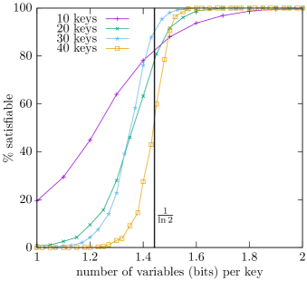
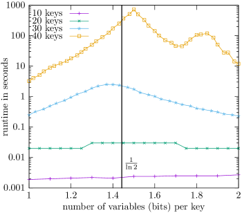
Figure 1: Left, the satisfiability threshold for MPHFs with $10$, $20$, $30$, and $40$ keys. The horizontal axis shows the number of bits per key. The vertical axis is the fraction of runs (out of $2400$) that were satisfiable. The bold vertical line represents the MPHF information-theoretic limit for large sets. Right, the average runtime to build MPHFs with $10$, $20$, $30$, and $40$ keys. The vertical axis shows the runtime in seconds using a logscale.

Encodings

The encoding of a problem into SAT can have a big impact on the performance of SAT solvers. We observed this for MPHF as well. An often used heuristic for an effective encoding is to minimize the sum of the number of variables and the number of clauses. This heuristic is, for example, used in the most-commonly applied SAT-preprocessing technique—bounded variable elimination (?). We thus focused our initial efforts on designing a compact encoding.

If $n$, the number of keys, is a power of 2, then the encoding only requires the following all-different constraint, which we need to encode in conjunctive normal form:

$$\bigwedge_{1\leq i<j\leq n}{L_{1}(y_{i})}\dots L_{k}(y_{i})\neq{L_{1}(y_{j})}\dots L_{k}(y_{j}).$$ (1)

Additionally, if the number of keys is not a power of 2, then we need a constraint stating that none of the elements should be mapped to values larger than $n$.

The first and most compact encoding of the all-different constraint used in our experiments introduces auxiliary variables $e_{a,b}$ with $a,b\in\{x_{1},\overline{x}_{1},\dots,x_{m},\overline{x}_{m}\}$ that denote that literals $a$ and $b$ are equal. So $e_{a,a}=1$, $e_{a,\overline{a}}=0$, and $e_{a,b}=e_{b,a}$. These variables are used to construct the clauses

$$\bigwedge_{1\leq i<j\leq n}(\overline{e}_{L_{1}(y_{i}),L_{1}(y_{j})}\lor\dots\lor\overline{e}_{L_{k}(y_{i}),L_{k}(y_{j})}).$$ (2)

Intuitively, these clauses state that the keys for distinct elements $y_{i}$ and $y_{j}$ need to differ in at least one bit.

Notice that we only need such $e_{a,b}$ variables if for some pairs of elements $y$ and $y^{\prime}$ and some $i$ holds that $L_{i}(y)=a$ and $L_{i}(y^{\prime})=b$. The intuitive meaning of the $e_{a,b}$ variables can simply be encoded using an XOR constraint:

$$e_{a,b}\oplus a\oplus b\equiv 1.$$ (3)

Although encoding ternary XOR constraints normally requires four clauses, we used only the two clauses with the positive literal $e_{a,b}$ as the two clauses with the negative literal $\overline{e}_{a,b}$ are blocked (?) and thus redundant. The resulting encoding has $\mathcal{O}(n^{2}\log_{2}(n))$ ternary clauses and $\mathcal{O}(n^{2})$ clauses of length $k$.

We also explored various other encodings since the results based on the above encoding were disappointing. The most effective encoding (for both complete and incomplete solvers) that we explored uses no auxiliary variables—in case the number of keys is a power of 2, we encode the constraint (1) as follows:

$$\!\bigwedge_{~{}1\leq i,j,l\leq n,i\neq j\!\!\!\!}\!\!\!\!\!\!\!\!\!\!{L_{1}(y_{i})}\dots L_{k}(y_{i})=l\rightarrow{L_{1}(y_{j})}\dots L_{k}(y_{j})\neq l.\!\!$$ (4)

In the above, ${L_{1}(y_{i})}\dots L_{k}(y_{i})=l$ denotes that the bit-vector interpretation of ${L_{1}(y_{i})}\dots L_{k}(y_{i})$, with ${L_{1}(y_{i})}$ being the most significant bit, equals the $l$th position in range $[n]$. E.g., $\langle{\tt 000}\rangle=1$ and $\langle{\tt 001}\rangle=2$. In case the number of keys is not a power of 2, we drop both literals that represent the most significant bits, i.e., $L_{1}(y_{i})$ and $L_{1}(y_{j})$, for all $l$ with $l+2^{k-1}>n$ and $l-2^{k-1}<1$.

When representing this encoding in conjunctive normal form, the number of clauses is cubic in $n$ and therefore much larger compared to the first encoding, which uses auxiliary variables. Also, the clauses are of length $2k$. It is therefore unlikely that one can use this encoding to construct MPHFs with hundreds of keys because solving almost any formula with over a million clauses is challenging for current state-of-the-art solvers. The encoding also produces many tautological clauses and duplicate literals, which are both discarded by our generator.

The cubic encoding turned out to be more effective compared to the compact encoding. For example, formulas with 32 keys and 46 variables can be solved with the cubic encoding with an average runtime of 4 seconds whereas the average solving time for formulas based on the compact encoding was 8.5 seconds. One explanation for the difference is that the cubic encoding enables more unit propagations. Consider again Example 1 and in particular the constraint stating that the bit-vectors of $y_{1}$ and $y_{3}$ must be different. In terms of variables it means that $\overline{x}_{1}x_{5}$ cannot be equal to $x_{3}x_{1}$. Under the assignment that makes $x_{3}$ true and $x_{5}$ false, we can deduce that $x_{1}$ must be true. Unit propagation on the cubic encoding will infer this. However, in the compact encoding we end up with the binary clauses $(\overline{e}_{x_{1},x_{3}}\lor\overline{e}_{\overline{x}_{1},x_{5}})$, $(e_{x_{1},x_{3}}\lor x_{1})$, and $(e_{\overline{x}_{1},x_{5}}\lor x_{1})$.

Other encodings of the all-different constraint of bit-vectors have been studied in the literature (?; ?), but the authors considered the case where the number of bit-vectors is significantly smaller than the range of the bit-vectors. For our application, however, the number of bit-vectors and their range is equal or similar.

We observed that SAT encodings of MPHF problems with $m\geq\lceil n/\ln 2\rceil$ have a high probability of being satisfiable (in the range of $n$ up to 40 used in the evaluation) and that a phase transition pattern can be observed near the information-theoretic limit of constructing MPHFs. We experimented with a range of different SAT encodings and SAT solvers, but the current state-of-the-art tools are not powerful enough to practically construct MPHFs with more than 40 elements near the theoretic limit.

Experimental Evaluation

We evaluated the effectiveness of our SAT-based approach to constructing MPHFs near the information-theoretic limit. The encoding and decoding tools are available at https://github.com/weaversa/MPHF. We used cube-and-conquer (?) to solve the resulting formulas as this approach demonstrated strong performance on the hardest MPHF instances. Cube-and-conquer splits a given problem into multiple subproblems, which are solved by a “conquer” solver. We used glucose 3.0 (?) as conquer solver. All mentioned runtimes are the sum of splitting the problem and the solving time by the conquer solver on a single core of a Xeon CPU E5-2650.

Figure 1 (left) shows the results for $10$, $20$, $30$, and $40$ random keys with the number of bits per key between 1 and 2. Each point shows the fraction of satisfiable formulas averaged over 2400 instances for each number of keys ($n$) and number of variables ($m$). The bold vertical line denotes the information-theoretic limit.

The observed phase transition from UNSAT to SAT becomes more and more sharper when increasing the number of keys. Moreover, the curve based on 40 keys appears to be almost symmetric (rotation by 180 degrees) in the point at 50% at the information-theoretic limit for large $n$. Recall that the information-theoretic limit $\alpha_{40}=1.343$. Hence the phase transition happens slightly after the limit. We analyzed the results and noticed various instances that did not use all $m$ variables. If one or more variables are missing, then the formula is more likely to be unsatisfiable. The observed phase transition for $n=40$ is much closer to $\alpha_{40}$ when only considering the instances that use all $m$ variables.

Our results show that the SAT-based approach is able to construct close to space-optimal MPHFs for the limited number of keys considered in the experimental evaluation. They also suggest that the curve would further sharpen when increasing the number of keys. To the best of our knowledge, this is the first approach that can construct close to space-optimal MPHFs for 40 keys in reasonable time.

Unfortunately, experiments with off-the-shelf SAT solvers on the encodings exhibit exponential runtime on the number of keys as shown in Figure 1 (right). The runtime bump near 1.8 for $40$ keys is due to the lack of subproblems that are generated. Generating more subproblems for these instances would reduce the runtime (combined splitting and solving time). The formulas for 40 keys at the observed phase transition require on average about 800 seconds, although for some instances solving takes a few hours. In contrast, the hardest instance for 30 keys can be solved in a several seconds. Hence, larger runs that may sharpen the logistic curve could not be completed. We experimented with both complete and incomplete state-of-the-art solvers, including probsat (?). Whether there exists an encoding that is more amenable to SAT solvers is left for future work.

A $1.83n$ MPHF Construction

The second MPHF construction, which allows building MPHFs with approximately $1.83n$ bits per key, also uses a universal family of $k$ hash functions and returns a bit-vector of $m$ bits. However, obtaining the index for a key is quite different. Instead of computing the index bit by bit, the second MPHF approach computes which hash function should be used to obtain the index.

To build an MPHF for a set $Y$ with $n$ elements, given a set of universal hash functions ${H_{1},...,H_{k}}$ each with range $[n]$, we first create a weighted bipartite graph $G=(Y,[n],E)$, where for all $y\in Y$ and for all $i\in[k],(y,H_{i}(y))\in E$, it holds that $\mathit{weight}(y,H_{i}(y))=i$.

Here, the weighted bipartite graph is created in such a way that the nodes on the left-hand-side (i.e., the left partition) represent elements of $Y$ and the right-hand-side nodes represent elements from $[n]$. The hash functions determine how every left-hand-side node is connected to $k$ right-hand-side nodes. That is, for each $y\in Y$, compute ${H_{1}(y),\dots,H_{k}(y)}$ and add edges from $y$ to the resulting nodes produced by the hash functions. The weight of each edge is assigned the index of the hash function used, that is, $\mathit{weight}(y,H_{i}(y))=i$.

The parameter $k$ should be chosen in a way that guarantees that $G$ possesses a perfect matching. A result by Frieze and Melsted (?) shows that, with high probability, $G$ will have a perfect matching when the degree of each left-hand-side node is at least three and the degree of each right-hand-side node is at least two. Newman and Shepp’s result (?) on the Double Dixie Cup Problem shows that the right-hand-side nodes will, with high probability, have degree two when the number of edges reaches $n(\ln n+\ln(\ln n))$. Hence, since every $H_{i}$ is used to hash $n$ keys, the optimal value for parameter $k$ is $max(3,\ln n+\ln(\ln n))$.

Let $M$ be a minimum-weight perfect matching of $G$. $M$ can be found in $\mathcal{O}(n^{3})$ steps using the Hungarian Algorithm (?). $M$ is also the bijective mapping of the MPHF being built. Since $G$ fits Parviainen’s proposed “Case II” (?), $M$ has weight approximately $1.83n$, asymptotically, which was determined experimentally.

The mapping $M$ is stored in a space-efficient retrieval structure such that, for each $y$, if $H_{i}(y)\in M$ then store $((i,y),1)$ (definite presence) and for each $j<i$ store $((j,y),0)$ (definite absence). Such a retrieval structure can be created in $\mathcal{O}((1.83n)^{3})$ steps, takes up one bit of space per element stored, and can be accessed in a small constant number of steps (?). It’s worth noting that both the Hungarian Algorithm and the retrieval structure construction process can benefit from sharding the input into small sets (which can all be processed in parallel), meaning that the MPHF can be created more efficiently than two $\mathcal{O}(n^{3})$ steps, though at a determinable, yet practically small loss to space efficiency. The long-term storage of this MPHF construction is equivalent to the size of the retrieval structure which will be approximately $1.83n$.

To find the mapping from $y$ to its corresponding index, query the retrieval structure with $(i,y)$, starting with $i=1$ and increment until $1$ is given. Then, the index for $y$ is $H_{i}(y)$.

Example 2.

We provide a detailed example of building an MPHF by storing a minimum weight perfect matching of a bipartite graph in the solution of a $k$-XORSAT instance. Let $Y$ be the set $\{y_{1},y_{2},y_{3},y_{4},y_{5}\}$, resulting in $n=5$ and $k=max(3,\ln 5+\ln(\ln 5))=3$. First, the $k$ hash functions are evaluated on all elements of $Y$, producing the following table.

	$H_{1}$	$H_{2}$	$H_{3}$
$y_{1}$	1	5	2
$y_{2}$	2	4	5
$y_{3}$	1	3	4
$y_{4}$	1	3	1
$y_{5}$	5	3	3

Next, a bipartite graph is built from the table by adding for each element in $Y$ an edge from the element to the results of the hash functions. Thus, for instance, $y_{1}$ is connected to $1$, $5$, and $2$.

The weight of each edge is equal to the index of the hash function used. For example, edge $(y_{1},1)$ has weight $1$ and edge $(y_{2},5)$ has weight 3. The Hungarian Algorithm is now used to find a minimal weight perfect matching of the bipartite graph. One such matching (which has weight $8$) is given below.

	$H_{1}$	$H_{2}$	$H_{3}$
$y_{1}$		5	2
$y_{2}$		4	5
$y_{3}$	1	3
$y_{4}$	1		1
$y_{5}$		3	3

This corresponds to the following matching:

The final step is to store the matching in an XORSAT filter. For this example, we store the following $8$ elements:

$((y_{1},1),1),$
$((y_{2},1),1),$
$((y_{3},1),0),$	$((y_{3},2),0),$	$((y_{3},3),1),$
$((y_{4},1),0),$	$((y_{4},2),1),$
$((y_{5},1),1)$.

Elements are stored in the filter in the way proposed by Weaver et al. (?), where the first part of the tuple is the element being filtered on and the second part is one bit of metadata to store (treating the filter like a dictionary of one-bit items).

Let $t$ denote the number of tuples, in this case 8. We construct the XORSAT filter using two hash functions with range $[t]$. We limit the number of hash functions for readability, but use 5 hash functions in practice to generate an XORSAT filter with high efficiency.

tuple	$H_{1}$	$H_{2}$	XOR constraint
$(y_{1},1)$	3	6	$x_{3}\oplus x_{6}\equiv 1$
$(y_{2},1)$	5	1	$x_{5}\oplus x_{1}\equiv 1$
$(y_{3},1)$	4	8	$x_{4}\oplus x_{8}\equiv 0$
$(y_{3},2)$	2	3	$x_{2}\oplus x_{3}\equiv 0$
$(y_{3},3)$	5	4	$x_{5}\oplus x_{4}\equiv 1$
$(y_{4},1)$	8	7	$x_{8}\oplus x_{7}\equiv 0$
$(y_{4},2)$	2	7	$x_{2}\oplus x_{7}\equiv 1$
$(y_{5},1)$	4	3	$x_{4}\oplus x_{3}\equiv 1$

The conjunction of the XOR constraints is satisfiable, for example by assigning the truth value ${\tt 1}$ to the variables $x_{2}$, $x_{3}$, and $x_{5}$, and the truth value ${\tt 0}$ to the other variables. We thus store the bit vector $\langle{\tt 01101000}\rangle$, using 8 bits for 5 elements.

The index of an element of $Y$ is determined by querying the filter a number of times, stopping when it returns $1$. In this example, to determine the index of $y_{3}$, we first query the filter with $(y_{3},1)$ and obtain the hashes $4$ and $8$. Thus, the filter will return $0$ because it has 0 at the positions 4 and 8, and $0\oplus 0\equiv 0$. Next, we query the filter with $(y_{3},2)$. The filter will again return $0$. Finally, we query the filter with $(y_{3},3)$. Now it will return $1$. This means the MPHF index of $y_{3}$ is $H_{3}(y_{3})=4$.

Proof of Concept

We provide some experimental results of building and testing the $1.83n$ MPHF construction. To this end, we wrote a tool that is composed of implementations of a minimum-weight bipartite perfect matcher and an XORSAT filter (?). All runs were performed on an Amazon EC2 instance of type m5.4xlarge. Such an instance has 16 cores, 64 GiB of memory, and currently costs 0.768 USD per hour.

Table 2: Runtime in seconds to compute the minimum-weight bipartite perfect matching on $n$ keys, per the construction described above.

$2^{9}$	$2^{10}$	$2^{11}$	$2^{12}$	$2^{13}$	$2^{14}$	$2^{15}$	$2^{16}$	$2^{17}$	$2^{18}$	$2^{19}$
$<$$1$	$<$$1$	$<$$1$	$<$$1$	$<$$1$	$1$	$2$	$9$	$32$	$134$	$566$

The results in Table 2 show that it will not be practical to build a large MPHF without blocking (or sharding) the input and solving each block independently. The trade-off here is that, in exchange for being able to build MPHFs for very large sets, blocking slightly decreases the space efficiency of the MPHF due to the need to store extra information relating to block sizes. Table 2 also gives some insight into appropriate block sizes for MPHFs: a block size between $2^{13}$ and $2^{14}$ allows blocks to be built in about one second.

Table 3: Achieved bits per key (BPK) and seconds taken to compute a blocked MPHF on $n$ keys, per the construction described above. Size refers to the number of kilobytes in the resulting MPHF. Cost of building is in USD. Query speed is in nanoseconds per query.

	Build Time				Query
$n$	1 Core	16 Cores	BPK	Cost	Speed
$2^{15}$	$3$	$<1$	1.85	0.00	172
$2^{16}$	$6$	$<1$	1.85	0.00	168
$2^{17}$	$14$	$2$	1.85	0.00	165
$2^{18}$	$28$	$3$	1.85	0.00	167
$2^{19}$	$55$	$4$	1.85	0.00	167
$2^{20}$	$114$	$8$	1.85	0.00	167
$2^{21}$	$228$	$15$	1.85	0.00	167
$2^{22}$	$450$	$30$	1.85	0.01	170
$2^{23}$	$903$	$59$	1.85	0.01	191
$2^{24}$	$1\,816$	$118$	1.85	0.03	225
$2^{25}$	$3\,503$	$228$	1.85	0.05	211
$2^{26}$	$7\,238$	$472$	1.85	0.10	221
$2^{27}$	$14\,465$	$952$	1.85	0.20	244
$2^{28}$	$28\,991$	$1\,920$	1.85	0.41	335
$2^{29}$	$57\,861$	$3\,892$	1.85	0.82	420
$2^{30}$	$120\,088$	$8\,346$	1.85	1.78	552

In Table 3, to maintain high XORSAT-filter efficiency up into the billions of keys, the XORSAT-filter parameters were raised from those suggested by Weaver et al. (?) to a block size of $4608$. We also used the sparse vector generation method proposed by Dietzfelbinger and Walzer (?). As expected, each run generated a weighted bipartite graph with a minimum weight of $1.831n$, so any loss in space efficiency is due to extra information stored about the MPHF blocking scheme and inefficiencies in the resulting XORSAT filters.

Recent practical improvements to the construction of space-efficient retrieval structures, such as those proposed by Dietzfelbinger and Walzer (?), would likely improve the results given here (shorter build time) and we plan to evaluate them in future work.

We performed a comparison between our approach and the state-of-the-art. Specifically, we used the benchmphf tool to generate MPHFs for $2^{30}$ elements. The benchmphf tool supports the EMPHF (?), HEM (?), CHD (?), and Sux4j implementations. Our results were similar to those reported by Limasset et al. (?) with construction time between $400$ and $2000$ seconds, bits per key between $2.90$ and $4.22$, and query time between $250$ to $1000$ nanoseconds per query. For $2^{30}$ elements, our implementation achieved $1.85$ bits per key, took $120000$ seconds (sequentially) to build, and has a query time of roughly $550$ nanoseconds per query.

Perfect Hash Functions

Our paper focuses on MPHFs, but the same techniques can also be used to construct (non-minimal) perfect hash functions (PHFs). We already observed for the SAT-based approach that increasing the number of variables (i.e, enlarging the distance with respect to the information-theoretic limit) reduces the costs to build a MPHF. Alternatively, one can reduce the costs by increasing the range to which keys are mapped and thus allow gaps.

When considering the $1.83n$ MPHF construction reworked for PHFs, the ratio of right-hand-side nodes to left-hand-side nodes in the bipartite graph will be greater than $1$. How does this effect the minimum weight of the graph? If the weight scales slowly as the ratio grows, the construction proposed here could also be used to build space-efficient PHFs.

Conclusions and Future Work

We presented two MPHF constructions. Our first construction achieves storage efficiency near the information-theoretic limit but has the drawback that SAT-solving techniques can currently only deal with instances up to 40 keys, which is still twice as much as previous (brute-force) approaches. Our second construction is practical in that it allows constructing MPHFs for large datasets for low costs and high query speeds. In fact, this is the most storage-efficient construction of all currently known practical MPHF constructions.

One of the exciting challenges for future work is to find out whether a SAT-solving tool can be developed that can construct MPHFs near the information-theoretic limit for a substantial number of elements. Such an approach would likely be based on local-search techniques as they tend to scale better on random problems, such as uniform random $k$-SAT formulas.

Our experiments revealed the surprising observation that a huge encoding without auxiliary variables achieves better results than more compact encodings. As stated earlier, this may be due to the increased propagation power of the cubic encoding. The development of an encoding with only $\mathcal{O}(n^{2}\log_{2}n)$ clauses with the same propagation power as the cubic encoding could further improve the results.

Acknowledgements

The second author is supported by the National Science Foundation (NSF) under grant CCF-1813993. The authors thank Benjamin Kiesl and the anonymous reviewers for their valuable input to improve the quality of the paper. The authors acknowledge the Texas Advanced Computing Center (TACC) at The University of Texas at Austin for providing HPC resources that have contributed to the research results reported within this paper.

References

- [Audemard and Simon 2009] Audemard, G., and Simon, L. 2009. Predicting learnt clauses quality in modern sat solvers. In IJCAI’09, 399–404. Morgan Kaufmann Publishers Inc.
- [Aumüller, Dietzfelbinger, and Rink 2009] Aumüller, M.; Dietzfelbinger, M.; and Rink, M. 2009. Experimental variations of a theoretically good retrieval data structure. In European Symposium on Algorithms, 742–751. Springer.
- [Balint and Schöning 2012] Balint, A., and Schöning, U. 2012. Choosing probability distributions for stochastic local search and the role of make versus break. In Cimatti, A., and Sebastiani, R., eds., Theory and Applications of Satisfiability Testing - SAT 2012, volume 7317 of Lecture Notes in Computer Science, 16–29. Springer.
- [Belazzougui et al. 2014] Belazzougui, D.; Boldi, P.; Ottaviano, G.; Venturini, R.; and Vigna, S. 2014. Cache-oblivious peeling of random hypergraphs. In Bilgin, A.; Marcellin, M. W.; Serra-Sagristà, J.; and Storer, J. A., eds., Data Compression Conference, DCC 2014, Snowbird, UT, USA, 26-28 March, 2014, 352–361. IEEE.
- [Belazzougui, Botelho, and Dietzfelbinger 2009] Belazzougui, D.; Botelho, F. C.; and Dietzfelbinger, M. 2009. Hash, displace, and compress. In European Symposium on Algorithms, 682–693. Springer.
- [Biere and Brummayer 2008] Biere, A., and Brummayer, R. 2008. Consistency checking of all different constraints over bit-vectors within a sat solver. In Proceedings of the 2008 International Conference on Formal Methods in Computer-Aided Design, FMCAD ’08, 28:1–28:4. Piscataway, NJ, USA: IEEE Press.
- [Botelho, Pagh, and Ziviani 2013] Botelho, F. C.; Pagh, R.; and Ziviani, N. 2013. Practical perfect hashing in nearly optimal space. Information Systems 38(1):108–131.
- [Dietzfelbinger and Pagh 2008] Dietzfelbinger, M., and Pagh, R. 2008. Succinct data structures for retrieval and approximate membership. In International Colloquium on Automata, Languages, and Programming, 385–396. Springer.
- [Dietzfelbinger and Walzer 2019a] Dietzfelbinger, M., and Walzer, S. 2019a. Constant-time retrieval with o (log m) extra bits. In STACS 2019. Schloss Dagstuhl-Leibniz-Zentrum fuer Informatik.
- [Dietzfelbinger and Walzer 2019b] Dietzfelbinger, M., and Walzer, S. 2019b. Dense peelable random uniform hypergraphs. In ESA 2019, volume 144 of LIPIcs, 38:1–38:16. Schloss Dagstuhl - Leibniz-Zentrum für Informatik.
- [Eén and Biere 2005] Eén, N., and Biere, A. 2005. Effective preprocessing in SAT through variable and clause elimination. In Bacchus, F., and Walsh, T., eds., SAT, volume 3569 of Lecture Notes in Computer Science, 61–75. Springer.
- [Fredman and Komlós 1984] Fredman, M. L., and Komlós, J. 1984. On the size of separating systems and families of perfect hash functions. SIAM Journal on Algebraic Discrete Methods 5(1):61–68.
- [Frieze and Melsted 2012] Frieze, A., and Melsted, P. 2012. Maximum matchings in random bipartite graphs and the space utilization of cuckoo hash tables. Random Structures & Algorithms 41(3):334–364.
- [Gableske 2014] Gableske, O. 2014. An Ising model inspired extension of the product-based MP framework for SAT. In Sinz, C., and Egly, U., eds., Theory and Applications of Satisfiability Testing - SAT 2014, volume 8561 of Lecture Notes in Computer Science, 367–383. Springer.
- [Genuzio, Ottaviano, and Vigna 2016] Genuzio, M.; Ottaviano, G.; and Vigna, S. 2016. Fast scalable construction of (minimal perfect hash) functions. In International Symposium on Experimental Algorithms, 339–352. Springer.
- [Heule et al. 2012] Heule, M. J. H.; Kullmann, O.; Wieringa, S.; and Biere, A. 2012. Cube and conquer: Guiding cdcl sat solvers by lookaheads. In Hardware and Software: Verification and Testing, 50–65. Springer.
- [Kautz and Selman 1996] Kautz, H. A., and Selman, B. 1996. Pushing the envelope: Planning, propositional logic and stochastic search. In Clancey, W. J., and Weld, D. S., eds., AAAI 96, 1194–1201. AAAI Press / The MIT Press.
- [Kuhn 1955] Kuhn, H. W. 1955. The Hungarian method for the assignment problem. Naval research logistics quarterly 2(1-2):83–97.
- [Kullmann 1999] Kullmann, O. 1999. On a generalization of extended resolution. Discrete Applied Mathematics 96-97:149–176.
- [Limasset et al. 2017] Limasset, A.; Rizk, G.; Chikhi, R.; and Peterlongo, P. 2017. Fast and scalable minimal perfect hashing for massive key sets. In 16th International Symposium on Experimental Algorithms, volume 11, 1–16.
- [Mehlhorn 1982] Mehlhorn, K. 1982. On the program size of perfect and universal hash functions. In 23rd Annual Symposium on Foundations of Computer Science (SFCS 1982), 170–175. IEEE.
- [Newman and Shepp 1960] Newman, D. J., and Shepp, L. 1960. The double dixie cup problem. The American Mathematical Monthly 67(1):58–61.
- [Parviainen 2004] Parviainen, R. 2004. Random assignment with integer costs. Combinatorics, Probability and Computing 13(1):103–113.
- [Porat 2009] Porat, E. 2009. An optimal Bloom filter replacement based on matrix solving. In Frid, A. E.; Morozov, A.; Rybalchenko, A.; and Wagner, K. W., eds., CSR 2009, volume 5675 of Lecture Notes in Computer Science, 263–273. Springer.
- [Seiden and Hirschberg 1994] Seiden, S. S., and Hirschberg, D. S. 1994. Finding succinct ordered minimal perfect hash functions. Information processing letters 51(6):283–288.
- [Surynek 2012] Surynek, P. 2012. An alternative eager encoding of the all-different constraint over bit-vectors. In Proceedings of the 20th European Conference on Artificial Intelligence, ECAI’12, 927–928. Amsterdam, The Netherlands, The Netherlands: IOS Press.
- [Weaver, Roberts, and Smith 2018] Weaver, S. A.; Roberts, H. J.; and Smith, M. J. 2018. XOR-satisfiability set membership filters. In International Conference on Theory and Applications of Satisfiability Testing, 401–418. Springer.