Electron swarm parameters in C2H2, C2H4 and C2H6: measurements and kinetic calculations

Abstract

This work presents swarm parameters of electrons (the bulk drift velocity, the bulk longitudinal component of the diffusion tensor, and the effective ionization frequency) in C2H_n, with $n=$ $246$, measured in a scanning drift tube apparatus under time-of-flight conditions over a wide range of the reduced electric field, $$1\text{\,}\mathrm{T}\mathrm{d}$\leq E/N\leq$1790\text{\,}\mathrm{T}\mathrm{d}$$ ($1\text{\,}\mathrm{T}\mathrm{d}$ = ${10}^{-21}\text{\,}\mathrm{V}\mathrm{m}^{2}$). The effective steady-state Townsend ionization coefficient is also derived from the experimental data. A kinetic simulation of the experimental drift cell allows estimating the uncertainties introduced in the data acquisition procedure and provides a correction factor to each of the measured swarm parameters. These parameters are compared to results of previous experimental studies, as well as to results of various kinetic swarm calculations: solutions of the electron Boltzmann equation under different approximations (multiterm and density gradient expansions) and Monte Carlo simulations. The experimental data are consistent with most of the swarm parameters obtained in earlier studies. In the case of C2H2, the swarm calculations show that the thermally excited vibrational population should not be neglected, in particular, in the fitting of cross sections to swarm results.

Keywords: electron swarm parameters, drift tube measurements, kinetic theory and computations.

1 Introduction

Acetylene (C2H2), ethylene (C2H4) and ethane (C2H6) are relatively simple hydrocarbons useful in specialized applications such as plasma-assisted combustion [1, 2, 3, 4, 5, 6], the fabrication of diamond-like films [7], graphene and carbon nanostructures [8], and particle detectors [9]. They are also involved in various chemical reactions in fusion plasmas [10], the Earth’s atmosphere [11] and in planetary atmospheric chemistry [12].

Knowledge on both electron collision cross sections and electron swarm parameters is needed for the quantitative modelling of plasmas. However, with the exception of the drift velocity, which was measured e.g. in [13, 14, 15, 16, 17] for C2H2, in [13, 18, 19, 16, 20, 21, 17, 22, 23] for C2H4, and in [13, 24, 25, 19, 15, 16, 17] for C2H6, further experimental transport and ionization coefficients have less frequently been reported for these hydrocarbon gases. Measurements of the longitudinal component of the diffusion tensor under time-of-flight (TOF) conditions were additionally reported in [14] for C2H2, [18, 19, 20] for C2H4, and [24, 19] for C2H6. Hasegawa and Date [13] also determined the effective ionization coefficient by the steady-state Townsend (SST) method for seven organic gases including acetylene, ethylene, and ethane. In addition to the drift velocity for C2H6, Kersten [25] measured the effective ionization coefficient under TOF conditions for a narrow range of the reduced electric field, $E/N$. Furthermore, measured data for the effective SST ionization coefficient have been reported e.g. in [26] for C2H2, in [27, 26] for C2H4, and in [28, 29, 30] for C2H6.

The aim of this work is (i) to determine the electron transport and ionization coefficients in C2H2, C2H4 and C2H6 gases in a wide range of $E/N$, (ii) to compare these results with those obtained in earlier investigations of these gases, and (iii) to compare the experimental data with those obtained from kinetic calculations and simulations using up-to-date electron collision cross section sets.

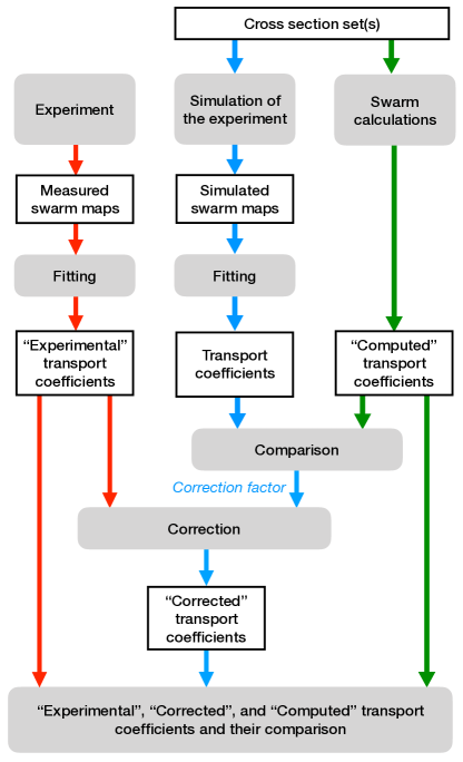
Figure 1: Graphical representation of the work reported in this article. The red arrows indicate the path from the measurements to the ’Experimental’ transport coefficients and ionization frequencies via fitting of the measured ’swarm maps’. Another ’Corrected’ set of experimental data is also derived based on a correction procedure which is aided by simulations of the experimental setup and related data acquisition (indicated by blue arrows) and by kinetic computations of the swarm parameters. The results of these calculations (’Computed’ transport coefficients) are also compared to the experimental data (green arrows).

The workflow of our studies can be followed with the aid of figure 1. The red arrows show the path to the ’Experimental transport coefficients’ including the effective ionization frequencies. The first step along this path consists of the measurements carried out with our scanning drift tube apparatus. This is a pulsed system, which is described in section 2. It records current traces generated by electrons collected from clouds that arrive after having flown over the drift region. The results of the experiments are the so-called ’swarm maps’ which are collections of these current traces for a number of drift gap length values. The swarm parameters are derived from the measured swarm maps via a fitting procedure that assumes that the current measured in the experiment is proportional to the electron density. For the fitting we use the theoretical form of the electron density in the presence of an electric field pointing in the $-z$ direction and under TOF conditions:

$$n_{\rm e}(z,t)=\frac{n_{0}}{(4\pi D_{\rm L}t)^{1/2}}\exp\biggl{[}\nu_{\rm eff}t-\frac{(z-Wt)^{2}}{4D_{\rm L}t}\biggr{]}.$$ (1)

This is the solution of the spatially one-dimensional (1D) continuity equation and represents a Gaussian pulse drifting along the $z$ direction with the bulk drift velocity, $W$, and diffuses along the centre-of-mass according to the bulk longitudinal component of the diffusion tensor $D_{\rm L}$. Here $n_{0}$ is the electron density at $z=0$ at time $t=0$, and $\nu_{\rm eff}$ is the effective ionization frequency. From the fitting procedure we obtain $W$, $D_{\mathrm{L}}$, and $\nu_{\mathrm{eff}}$. The application of the relation [31]

$$\frac{1}{\alpha_{\mathrm{eff}}}=\frac{W}{2\nu_{\rm eff}}+\sqrt{\left(\frac{W}{2\nu_{\rm eff}}\right)^{2}-\frac{D_{\rm L}}{\nu_{\rm eff}}}$$ (2)

allows us to derive the effective SST ionization coefficient, $\alpha_{\mathrm{eff}}$, as well.

The assumption that the measured current is proportional to the electron density is, in fact, an approximation, due to two reasons. First, the measured current is generated by moving charges in the detector of the system (see later). In our previous work [32] we have found that the detection sensitivity depends on the gas pressure and the collision cross sections, which both influence the free path of the electrons. This means that any variation of the energy distribution along the $z$ direction in the electron cloud may results in a distortion of the detected pulse and a deviation from the analytical fitting function (1) assumed. Second, the measured current is proportional to the electron flux consisting of the advective and diffusive component. The advective component is proportional to the electron density, where the coefficient of proportionality is the flux drift velocity, and the diffusive component is proportional to the gradient of the electron density. Using Ramo’s theorem [33], it can be shown that for the experimental conditions considered in the present work, the contribution of the diffusive component to the current is negligible compared to the contribution of the advective component, except in the early stage of the swarm development when the spatial gradients of the electron density are more significant.

The errors introduced by the first effect mentioned above can be quantified by a procedure, which is marked by blue arrows in figure 1. We carry out a (Monte Carlo) simulation of the electrons’ motion in the experimental system. This simulation generates the same type of swarm maps, which are obtained in the experiments, and a set of swarm parameters is derived via the same fitting procedure as in the case of experimental swarm maps. The transport coefficients and ionization frequencies obtained in this way are compared with the ’Computed’ ones, originating from kinetic swarm calculations. We note that (i) this comparison does not include any experimental data, (ii) the system’s simulations use the same cross section set as in the kinetic swarm calculations, and (iii) uncertainties of the used collision cross sections have little influence on the outcome of the comparison of the parameter sets obtained by swarm calculations and simulations of the experimental system. The result of this comparison is gas- and $E/N$-dependent correction factors that are applied to the experimental data, providing sets of ’Corrected’ experimental transport and ionization coefficients. Details are given below in section 4.

The two (raw and corrected) sets of experimental results are compared with swarm parameters derived from kinetic calculations based on solutions of the electron Boltzmann equation and on Monte Carlo simulations as described in detail in section 3. The application of these different approaches allows us to mutually verify the accuracy of the different methods and test the assumptions used by each method. The ’flow’ of this process is indicated by the green arrows in figure 1.

The manuscript is organized as follows: in section 2 we give a concise description of our experimental setup. A discussion of the various computational methods and the resulting swarm parameters is presented in section 3, and section 4 describes the correction procedure applied to the experimental data. It is followed by the discussion of the results in section 5. This section comprises the presentation of the present experimental results for each gas and their comparison with previously available measured data as well as the comparison between transport parameters and ionization coefficients computed using the various numerical methods and the present experimental data. Section 6 gives our concluding remarks and in the appendix we provide tabulated values of our experimental results.

2 Experimental system

The experiments are based on a ’scanning’ drift tube apparatus, of which the details have been presented in [34]. This apparatus has already been applied for the measurements of transport and ionization coefficients of electrons in various gases: argon, synthetic air, methane, deuterium [35] and carbon dioxide [36]. In contrast to previously developed drift tubes, our system allows for recording of ’swarm maps’ that show the spatio-temporal development of electron clouds under TOF conditions. The simplified scheme of our experimental apparatus is shown in figure 2.

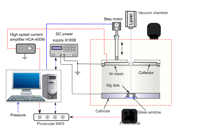
Figure 2: Simplified schematic of the scanning drift tube apparatus

The drift cell is situated within a vacuum chamber made of stainless steel. The chamber can be evacuated by a turbomolecular pump backed with a rotary pump to a level of about $1\text{\times}{10}^{-7}\text{\,}\mathrm{m}\mathrm{b}\mathrm{a}\mathrm{r}$. The pressure of the working gases inside the chamber is measured by a Pfeiffer CMR 362 capacitive gauge.

Ultraviolet light pulses ($1.7\text{\,}\mathrm{\SIUnitSymbolMicro J}$, $5\text{\,}\mathrm{n}\mathrm{s}$) of a frequency-quadrupled diode-pumped YAG laser enter the chamber via a feedthrough with a quartz window and fall on the surface of a Mg disk used as photoemitter. This disk is placed at the centre of a stainless steel electrode with 105 mm diameter that serves as the cathode of the drift cell. The detector that faces the cathode at a distance $L_{1}$ consists of a grounded nickel mesh (with $T=$88\text{\,}\mathrm{\char 37\relax}$$ ’geometric’ transmission and 45 lines/inch density) and a stainless steel collector electrode that is situated at a distance of $L_{2}=$1\text{\,}\mathrm{mm}$$ behind the mesh.

Electrons emitted from the Mg disk fly towards the collector under the influence of an accelerating voltage that is applied to the cathode. This voltage is established by a BK Precision 9185B power supply. Its value is adjusted according to the required $E/N$ for the given experiment and the actual value of the gap ($L_{1}$) during the scanning process, where $E/N$ is ensured to be fixed. The current of the detector system is generated by the moving charges within the mesh-collector gap: according to the Shockley-Ramo theorem [33, 37, 38] the current induced by an electron moving in a gap between two plane-parallel electrodes with a velocity $v_{z}$ perpendicular to the electrodes is $I=-e_{0}v_{z}/L$, where $-e_{0}$ is the charge of the electron and $L$ is the distance between the electrodes ($L=L_{2}$ in our case). Accordingly, in our setting the measured current at a given time $t$ is

$$I(t)=c\sum_{k}v_{z,k}(t)\,,$$ (3)

where $c$ is a constant. The summation goes over all electrons being present in the volume bounded by the mesh and the collector at time $t$, and $v_{z,k}$ is the velocity component of the $k$-th electron in $z$ direction.

Electrons entering the detector region (the gap between the nickel mesh and the collector) contribute to the measured current until their first collisions with the gas molecules, as these collisions randomise the angular distribution of their velocities. Therefore, the free path of the electrons plays a central role in the magnitude of the current. For conditions when this free path is longer than the detector gap, the electron sticking property of the collector surface plays a crucial role too, as reflected electrons generate a current contribution with an opposite sign with respect to that generated by the ’incoming’ electrons. According to the above effects, which have been explored to some details in [32], the sensitivity of the detector changes with the nature of the gas (magnitudes and energy dependence of the electron collision cross sections), the pressure, as well as the energy distribution of the electrons. This dependence is the primary reason which calls for a correction of the measured transport and ionization coefficients as discussed in more details in section 4.

The collector current is amplified by a high speed current amplifier (type Femto HCA-400M) connected to the collector, with a virtually grounded input, and is recorded by a digital oscilloscope (type Picoscope 6403B) with sub-ns time resolution. Data collection is triggered by a photodiode that senses the laser light pulses. The low light pulse energy necessitates averaging over typically $20\,000150\,000$ pulses. The experiment is fully controlled by a computer using LabView software.

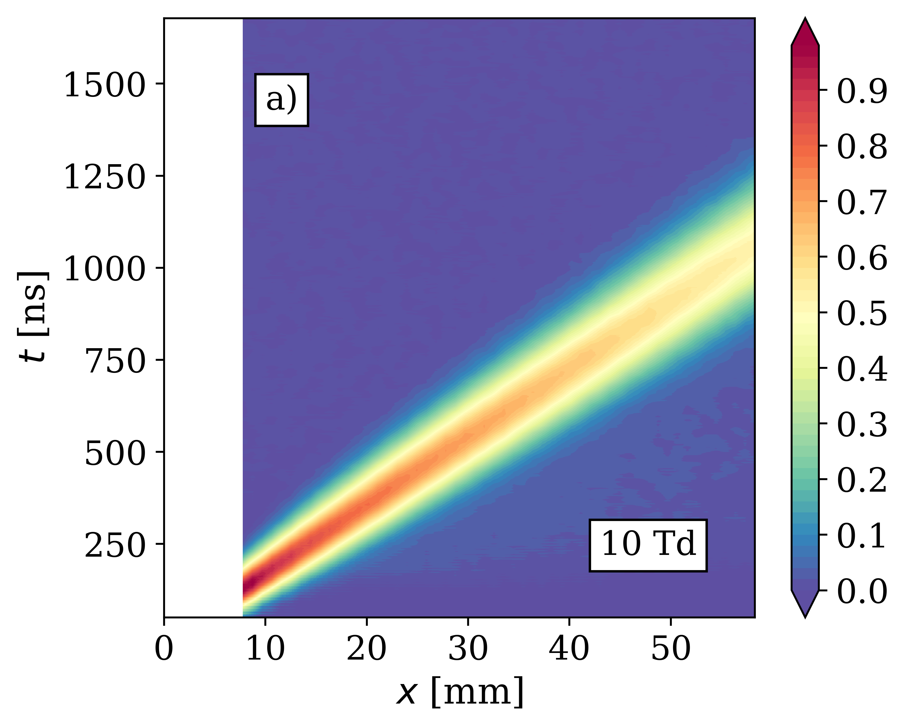
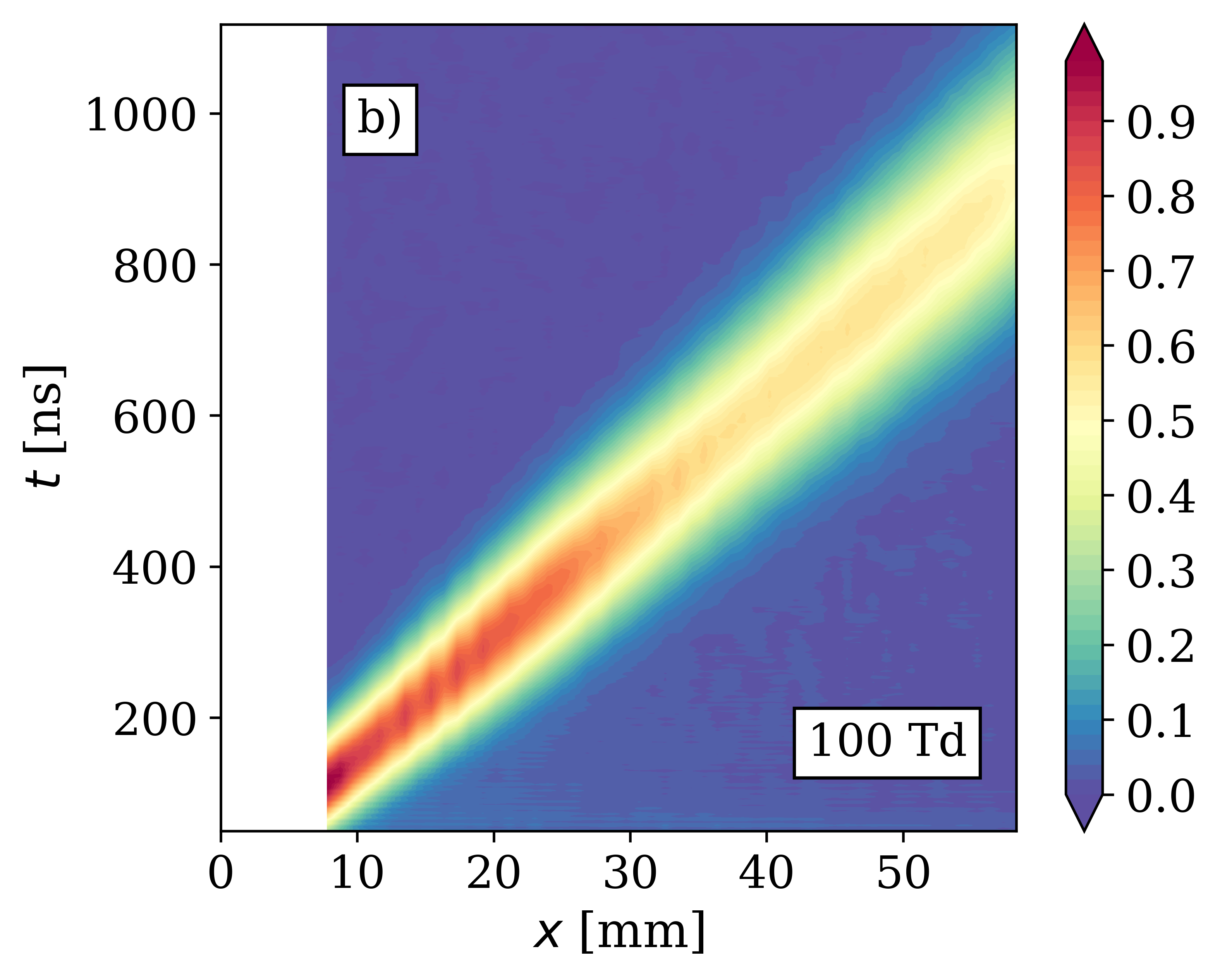
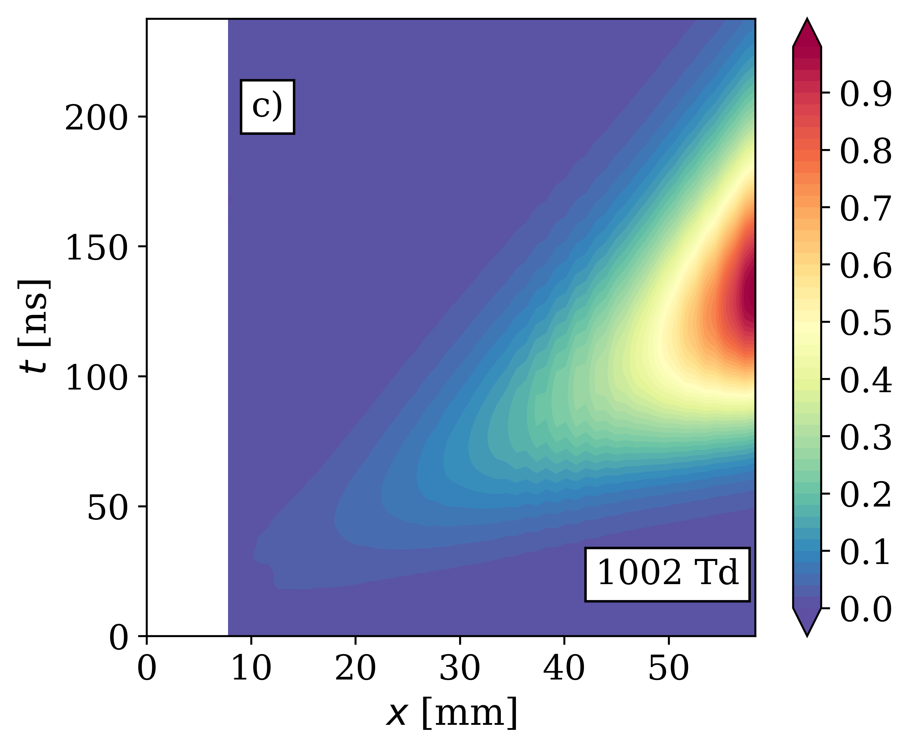
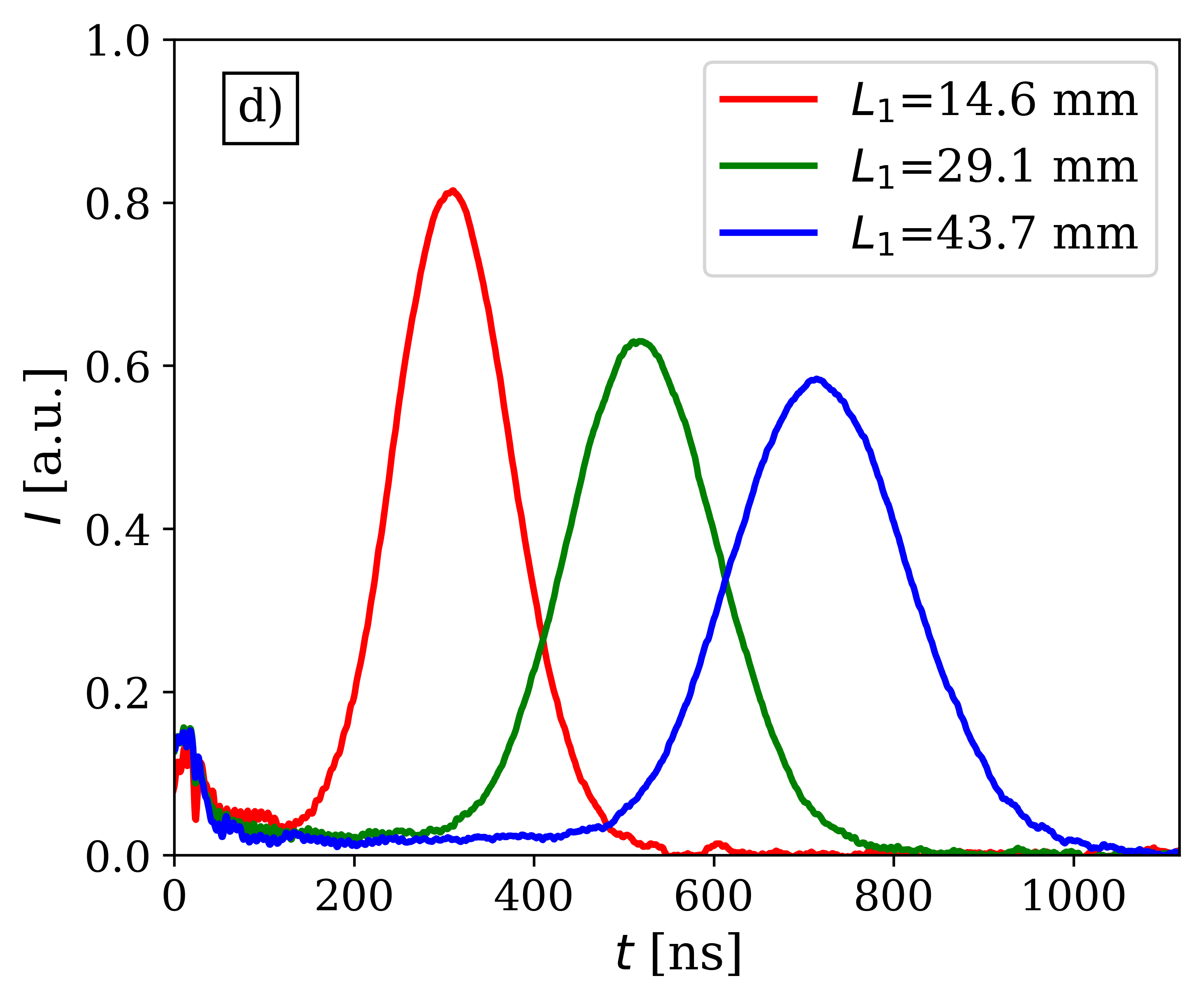
Figure 3: (a-c) Swarm maps recorded in C2H6 for different values of $E/N$, as indicated. (d) Vertical cuts of the swarm map of (b), which are the measured current traces at the drift length values given in the legend. The pulses have nearly Gaussian shapes. The ’shift’ of the pulses with increasing drift length ($L_{1}$) is the manifestation of the drift, while their widening is due to (longitudinal) diffusion. As ionization in C2H6 is weak at $E/N$ = $100\text{\,}\mathrm{T}\mathrm{d}$, the amplitude of the pulses decreases with increasing $L_{1}$ due to the widening of the pulse.

During the course of the measurements current traces are recorded for several values of the gap length. The grid and the collector are moved together by a step motor connected to a micrometer screw mounted via a vacuum feedthrough to the vacuum chamber. The distance between the cathode and the mesh, i.e. the ’drift length’, can be set within a range of $L_{1}$ = $7.858.3\text{\,}\mathrm{m}\mathrm{m}$. Here, we use 53 positions within this domain.

Sequences of the measured current traces are subsequently merged to form ’swarm maps’, which provide information about the spatio-temporal development of the electron cloud. Figure 3(a)-(c) illustrates such swarm maps, obtained in experiments on C2H6, for different values of the reduced electric field. The qualitative behaviour of the swarm is directly seen in these pictures: the slope of the region with appreciable current indicates the drift of the cloud, the widening of this region is related to (longitudinal) diffusion, while an increasing amplitude (as seen in panel (c)) is an indication of ionization. Figure 3(d) displays vertical ’cuts’ of the map shown in panel (b), for $E/N$ = $100\text{\,}\mathrm{T}\mathrm{d}$. These cuts are, actually, the current traces recorded in the measurements at different gap length values.

3 Simulation of the electron swarm

The experimental studies of the electron transport are supplemented by numerical modelling and simulation. In addition to Monte Carlo (MC) simulations, three different methods are applied to solve the Boltzmann equation (BE) for electron swarms in a background gas with density $N$ and acted upon by a constant electric field, $\vec{E}$: a multiterm method for the solution of the time-independent Boltzmann equation under spatially homogeneous and SST conditions, respectively, and the $S_{n}$ method applied to a density gradient expansion of the electron velocity distribution function (EVDF). They differ in their initial physical assumptions and in the numerical algorithms used and provide different properties of the electron swarms.

Details of the different Boltzmann equation methods, as well as main aspects of the MC simulation have been discussed in [36], and we just provide a brief discussion below.

In the following, the electric field is parallel to the $z$ axis and points in the negative direction, $\vec{E}=-E\vec{e}_{z}$, and $\theta$ is the angle between $\vec{v}$ and $\vec{E}$. Moreover, we assume that the spatial and time scales, respectively, exceed the energy relaxation length and time, such that the transport properties of the electrons do not change with time $t$ and distance $z$ any longer. That is, the electrons have reached a hydrodynamic regime characterizing a state of equilibrium of the system where the effects of collisions and forces are dominant and the EVDF, $f(\vec{r},\vec{v},t)$, has lost any memory of the initial state.

We base our studies on the electron collision cross section sets from Song et al. [39] for acetylene, Fresnet et al. [40] for ethylene and Shishikura et al. [24] for ethane. The cross sections for acetylene and ethane were extended to electron kinetic energies, $\epsilon$, of $1000\text{\,}\mathrm{e}\mathrm{V}$ by fitting a function with a $\log(\epsilon)/\epsilon$ dependence, according to the Born-Bethe high-energy approximation, to the tail of the original cross sections.

The C2H2 data set includes the momentum transfer cross section for elastic collisions, three vibrational cross sections for single quanta excitation of modes $v_{1}/v_{3}$, $v_{4}/v_{5}$ and $v_{2}$ (the first two unresolved) and one vibrational cross section for two quanta excitation of $v_{4}+v_{5}$, three electronic excitation cross sections, the total electron-impact ionization cross section and the total dissociative electron attachment cross section for C2H2 leading to the formation of C2H-, H- and C2-, respectively.

The C2H4 data set includes the momentum transfer cross section, two lumped vibrational cross sections with thresholds at $0.118\text{\,}\mathrm{e}\mathrm{V}0.365\text{\,}\mathrm{e}\mathrm{V}$, three electronic excitation cross sections, the total electron ionization cross section and a collision cross section for electron attachment.

Finally, the C2H6 set of collision cross sections includes the momentum transfer cross section, three lumped vibrational cross sections with thresholds at $0.112\text{\,}\mathrm{e}\mathrm{V}0.167\text{\,}\mathrm{e}\mathrm{V}0.36\text{\,}\mathrm{e}\mathrm{V}$, two electronic excitation cross sections, the total electron ionization cross section and an electron attachment cross section.

All of the above cross section sets were developed neglecting the population of thermally excited vibrational states and superelastic processes. The implications of this approximation are discussed in section 5.4.

3.1 Boltzmann equation methods

3.1.1 Multiterm method for spatially homogeneous conditions

In this approach, to describe $f(\vec{r},\vec{v},t)$ (abbreviated by BE 0D in the figures shown in section 5), we consider that the EVDF is spatially homogeneous (0D) and the electron density changes exponentially in time according to $n_{\mathrm{e}}(t)\propto\exp(\nu_{\mathrm{eff}}t)$ at the scale of the swarm. Here, the effective ionization frequency $\nu_{\mathrm{eff}}=\nu_{\rm i}-\nu_{\rm a}$ is the difference of the ionization ($\nu_{\rm i}$) and attachment ($\nu_{\rm a}$) frequencies. In this case we can neglect the dependence of $f$ on the space coordinates and write the EVDF under hydrodynamic conditions as

$$f(\vec{v},t)=\hat{F}(\vec{v})n_{\mathrm{e}}(t).$$ (4)

The corresponding microscopic and macroscopic properties of the electrons are determined by the time-independent, spatially homogeneous Boltzmann equation for $\hat{F}(\vec{v})$. As this distribution is symmetric around the field direction, it can be expanded with respect to the angle $\theta$ in Legendre polynomials $P_{n}(\cos\theta)$ with $n\geq 0$. Substituting this expansion in the Boltzmann equation leads to a hierarchy of partial differential equations for the coefficients $\hat{f}_{n}(v)$ of this expansion. The resulting set of equations with typically eight expansion coefficients is solved employing a generalized version of the multiterm solution technique for weakly ionized steady-state plasmas [41] adapted to take into account the ionizing and attaching electron collision processes.

Using the computed expansion coefficients $\hat{f}_{n}(v)$, we obtain the effective ionization frequency, $\nu_{\mathrm{eff}}$, and the flux drift velocity

$$w=-\mu E\,,$$ (5)

where $\mu$ is the flux mobility. Explicit formulas of these transport parameters obtained by the BE 0D method can be found in [36].

3.1.2 Multiterm method for SST conditions

This approach to describe the EVDF (abbreviated by BE SST in the figures shown in section 5) takes into account that $f(\vec{r},\vec{v},t)$ has reached SST conditions so that the mean transport properties of the electrons are time-independent, do not vary with position any longer, and the electron density assumes an exponential dependence on the distance according to $n_{\mathrm{e}}(z)\propto\exp(\alpha_{\mathrm{eff}}z)$. Thus, we can neglect the dependence of $f$ on time and write the EVDF under SST conditions as

$$f(z,\vec{v})=\tilde{F}^{(\rm S)}(\vec{v})n_{\mathrm{e}}(z),$$ (6)

where the upper index (S) denotes SST conditions. In accordance with the procedure described in section 3.1.1, the corresponding microscopic and macroscopic properties of the electrons are determined by the steady-state, spatially homogeneous Boltzmann equation for $\tilde{F}^{(\rm S)}(\vec{v})$. Since this distribution is again symmetric around the direction of the field, it can be expanded in Legendre polynomials $P_{n}(\cos\theta)$ with $n\geq 0$. The substitution of this expansion into the Boltzmann equation leads to a set of partial differential equations for the expansion coefficients $\tilde{f}^{(\rm S)}_{n}(v)$, which is solved efficiently by a modified version of the multiterm method [41] adapted to treat SST conditions [36].

In this approach, the effective SST ionization coefficient is directly given by

$$\alpha_{\mathrm{eff}}=\frac{\nu_{\mathrm{eff}}^{(\rm S)}}{v_{\mathrm{m}}^{(\rm S)}}.$$ (7)

Here, $\nu_{\mathrm{eff}}^{(\rm S)}$ and $v_{\mathrm{m}}^{(\rm S)}$ are the effective ionization frequency and mean velocity at SST conditions, respectively, which are calculated by means of the computed expansion coefficients $\tilde{f}_{n}^{(\rm S)}(v)$ [36].

3.1.3 Density gradient representation

When ionization or attachment processes become important in TOF experiments, the electron swarm can no longer be considered homogeneous and the electron density gradients become significant.

This approach to describe the electron swarm at hydrodynamic conditions (labelled as BE DG below) is based on an expansion of the EVDF with respect to space gradients of the electron density $n_{\mathrm{e}}$, of consecutive order. In this case, $f$ depends on $(\vec{r},t)$ only via the density $n_{\mathrm{e}}(\vec{r},t)$ and can be written as an expansion on the gradient operator $\nabla$ according to

$$f(\vec{r},\vec{v},t)=\sum_{j=0}F^{(j)}(\vec{v})\stackrel{{\scriptstyle j}}{{\odot}}(-\nabla)^{j}n_{\mathrm{e}}(\vec{r},t)\,,$$ (8)

where the expansion coefficients $F^{(j)}(\vec{v})$ are tensors of order $j$ depending only on $\vec{v}$, and $\stackrel{{\scriptstyle j}}{{\odot}}$ indicates a $j$-fold scalar product [42]. Note that the first coefficient $F^{(0)}(\vec{v})$ corresponds to the function $\hat{F}(\vec{v})$ above, for spatially homogeneous conditions (cf. section 3.1.1).

The expansion coefficients $F^{(j)}$ of order $j$ are obtained from a hierarchy of equations for each component, which all have the same structure and depend on the previous orders. In particular, to obtain the transport coefficients measured in TOF experiments, a total of five equations are required, namely for the expansion coefficients $F^{(0)}$, $F_{z}^{(1)}$, $F_{T}^{(1)}$, $F_{zz}^{(2)}$ and $F_{TT}^{(2)}$. In the present study, these equations are solved using a variant of the finite element method given in [43] in a $(v,\cos\theta)$ grid.

From the above expansion coefficients we obtain two sets of transport coefficients: the flux coefficients, neglecting the contribution of non-conservative processes and equivalent to those obtained by the BE 0D approach described in section 3.1.1, and the bulk coefficients including a contribution from ionization and attachment. The latter are, the bulk drift velocity,

$$W=w+\int\tilde{\nu}_{\mathrm{eff}}(v)F_{z}^{(1)}(\vec{v})\mathrm{d}\vec{v}$$ (9)

with $\tilde{\nu}_{\mathrm{eff}}(v)=vN[\sigma^{\rm i}(v)-\sigma^{\rm a}(v)]$ where $\sigma^{i}$ and $\sigma^{a}$ are, respectively, the ionization and attachment cross sections; and the longitudinal and transverse components of the diffusion tensor,

$$D_{\rm L} =\int v_{z}F_{z}^{(1)}(\vec{v})\mathrm{d}\vec{v}+\int\tilde{\nu}_{\mathrm{eff}}(v)F_{zz}^{(2)}(\vec{v})\mathrm{d}\vec{v}$$ (10)

$$D_{\rm T} =\frac{1}{2}\left\{\int v_{T}F_{T}^{(1)}(\vec{v})\mathrm{d}\vec{v}+\int\tilde{\nu}_{\mathrm{eff}}(v)F_{TT}^{(2)}(\vec{v})\mathrm{d}\vec{v}\right\}$$ (11)

Note that the first terms of the right-hand side of equations (9-11) are the flux component. Further details can be found in [36].

The effective or apparent Townsend ionization coefficient $\alpha_{\mathrm{eff}}$, as determined in SST experiments, can be computed from the TOF parameters using the relation [31]

$$\alpha_{\mathrm{eff}}=\frac{W}{2D_{\rm L}}-\sqrt{\left(\frac{W}{2D_{\rm L}}\right)^{2}-\frac{\nu_{\mathrm{eff}}}{D_{\rm L}}},$$ (12)

which is an equivalent way of writing equation (2).

3.2 Monte Carlo technique

In the MC simulation technique, we trace the trajectories of the electrons in the external electric field and under the influence of collisions. As the degree of ionization under the swarm conditions considered here is low, only electron-background gas molecule collisions are taken into account. The motion of the electrons with mass $m_{\mathrm{e}}$ between collisions is described by their equation of motion

$$m_{\mathrm{e}}\frac{\mathrm{d}^{2}\vec{r}}{\mathrm{d}t^{2}}=-e_{0}\vec{E}.$$ (13)

The electron trajectories between collisions are determined by integrating this equation numerically over time steps of duration $\Delta t$ ranging between $0.5\text{\,}\mathrm{ps}2.5\text{\,}\mathrm{ps}$ for the various conditions. While this procedure is totally deterministic, the collisions are handled in a stochastic manner. The probability of the occurrence of a collision is computed after each time step, for each of the electrons, as

$$P(\Delta t)=1-\exp{[-N\nu\sigma^{\rm T}(v)\Delta t]}.$$ (14)

The occurrence of a collision is determined by comparing $P(\Delta t)$ with a random number with a uniform distribution over the $(0,1)$ interval. The type of collision is also selected in a random manner taking into account the values of the cross sections of all possible processes at the energy of the colliding electron. For a more detailed description see [36].

The transport parameters (labeled as MC below) are determined as

$$W=\frac{\mathrm{d}}{\mathrm{d}t}\left[\frac{\sum_{j=1}^{N_{\mathrm{e}}(t)}z_{j}(t)}{N_{\mathrm{e}}(t)}\right]$$ (15)

and

$$w=\frac{1}{N_{\mathrm{e}}(t)}\sum_{j=1}^{N_{\mathrm{e}}(t)}\frac{\mathrm{d}z_{j}(t)}{\mathrm{d}t},$$ (16)

respectively for the bulk and flux drift velocities, where $N_{\mathrm{e}}(t)$ is the number of electrons in the swarm at time $t$. The bulk longitudinal and transverse components of the diffusion tensor are

$$D_{\rm L} =\frac{1}{2}\frac{\mathrm{d}}{\mathrm{d}t}\left[\langle z^{2}(t)\rangle-\langle z(t)\rangle^{2}\right]$$ (17)

$$D_{\rm T} =\frac{1}{4}\frac{\mathrm{d}}{\mathrm{d}t}\left[\langle x^{2}(t)+y^{2}(t)\rangle\right]\,,$$ (18)

and the effective ionization frequency is given by

$$\nu_{\mathrm{eff}}=\frac{\mathrm{d}\ln{(N_{\mathrm{e}}(t))}}{\mathrm{d}t}.$$ (19)

Furthermore, the effective SST ionization coefficient $\alpha_{\mathrm{eff}}$ is also calculated according to relation (12) using (15), (17) and (19).

All results of calculated electron swarm parameters presented in this work were additionally verified by independent Monte Carlo simulations and calculations based on multi-term solutions of the electron Boltzmann equation developed by the Belgrade group [44, 45]. For clarity, these results are not included in the figures shown in the next sections, but are available from the authors on request.

As it was already mentioned in the Introduction and is discussed in somewhat more detail in the next section, Monte Carlo simulations are also applied in the simulation of the electrons’ motion in the experimental system, assisting a correction procedure of the experimental data.

4 Correction of the experimental results

To quantify the effect caused by the variations of the electron energy distribution along the swarm, that in turn makes the detection sensitivity time-dependent, Monte Carlo simulations of the experimental system have been carried out for most of the sets of conditions $(p,E/N)$ in the experiments. These simulations generate swarm maps, similarly to those measured, and a set of swarm parameters is derived from these maps via exactly the same fitting procedure as in the case of the experimental data. The transport parameters and ionization frequencies obtained from the simulations of the setup are compared with those obtained from kinetic swarm calculations based on the solution of the electron Boltzmann equation, where the same electron collision cross section sets are used. Good agreement between the two sets of swarm parameters implies that the assumption made in the fitting of the experimental data, i.e. the use of the theoretical form (1) of $n_{\rm e}(z,t)$ as a fit to the measured data, is acceptable. In contrast, strong deviations indicate that this assumption is not applicable for the given condition. We note that no experimental data are involved in this procedure.

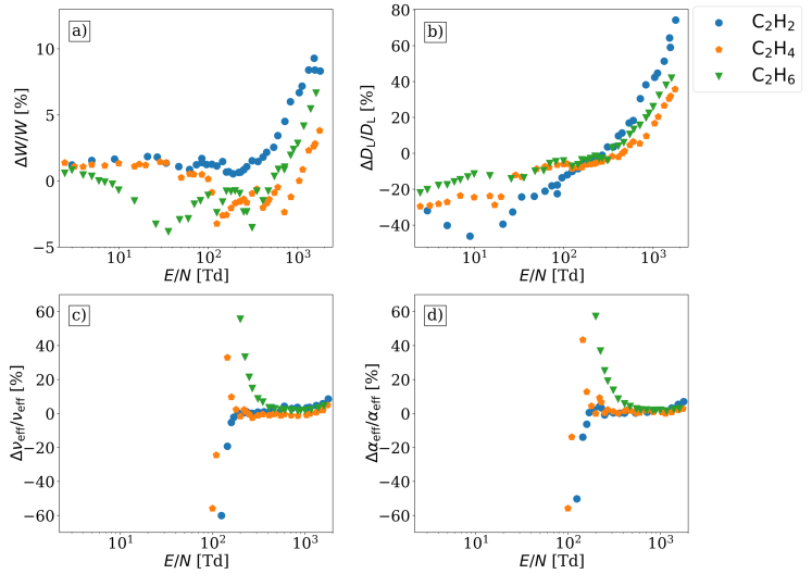
Figure 4: Deviations of the results between the swarm parameters obtained from the simulations of the experimental systems vs. the theoretical values. (a) Bulk drift velocity, (b) longitudinal component of the diffusion tensor, (c) effective ionization frequency, and (d) effective SST ionization coefficient. Applying these correction factors to the experimental results leads to the set of ’Corrected’ transport coefficients.

Results of this procedure for each of the gases and for the whole domain of $E/N$ are presented in figure 4. The panels correspond to the swarm parameters $W$, $D_{\rm L}$, $\nu_{\rm eff}$, and $\alpha_{\rm eff}$, respectively, and show the differences of each parameter derived by the simulation of the experimental system with respect to its theoretical value obtained from the BE solution.

In the case of the bulk drift velocity (figure 4(a), the error is in the few % range for most of the conditions, and it approaches $\approx$ $10\text{\,}\mathrm{\char 37\relax}$ at the highest $E/N$ values. This indicates that the determination of the bulk drift velocity values from the experimental data is quite relyable.

The situation turns out to be much worse for the longitudinal component of the diffusion tensor (figure 4(b)). Here, the error ranges from $\approx-$$40\text{\,}\mathrm{\char 37\relax}$ to $\approx+$$80\text{\,}\mathrm{\char 37\relax}$, depending on $E/N$. The $D_{\rm L}$ data can be considered to be acceptably accurate at intermediate $E/N$ values only. The much larger error of $D_{\mathrm{L}}$ with respect to that of $W$ can be explained by the fact that the distribution of the average electron energy along the swarm is inhomogeneous. In the close vicinity of the maximum of the spatial distribution of the electron density, the variation of the average energy along the swarm is comparatively small. However, by moving away from this maximum, the spatial variations of the average energy along the swarm increase. As the drift velocity is primarily determined by the position of the maximum of the spatial profile of the electron density while the diffusion is predominantly determined by the width of this distribution, it is clear that the width of the distribution is more affected by non-uniform sensitivity of the detector with respect to the average electron energy than the position of the maximum.

Regarding the effective ionization frequency (figure 4(c)) and the strongly related SST ionization coefficient (figure 4(d)), we observe small errors at high $E/N$ values, where ionization is appreciable. The error, on the other hand, grows high when $E/N$ approaches $\approx$ $100\text{\,}\mathrm{T}\mathrm{d}$, where both $\nu_{\rm eff}$ and $\alpha_{\rm eff}$ drop rapidly.

5 Results and discussion

The electron swarm parameters have been measured in a wide range of the reduced electric field, between $1\text{\,}\mathrm{T}\mathrm{d}1790\text{\,}\mathrm{T}\mathrm{d}$ at a gas temperature $T$ of $293\text{\,}\mathrm{K}$. In the following, results of our measurements are presented for the three hydrocarbon gases C2H2, C2H4, and C2H6. Besides the transport parameters and ionization coefficients resulting from the experiments via the fitting procedure described in section 1, we also present the corrected values of these data resulting from the procedure introduced in section 4. For each swarm parameter, we compare the present measured data with previous experimental results and with the results of the kinetic computations based on the solution of the electron Boltzmann equation or on MC simulations, obtained with the selected electron collision cross sections. The results for the flux parameters obtained by methods BE 0D, BE DG and MC overlap, and so do the bulk parameters obtained from the BE DG and MC methods.

5.1 Electron mobility

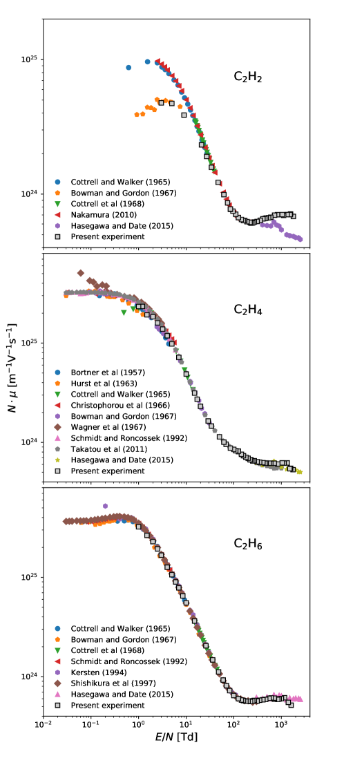
Figure 5: Mobility in C2H2, C2H4 and C2H6 obtained from drift velocity results: Bortner et al [23], Hurst et al [22], Cottrell and Walker [17], Christophorou et al [21], Bowman and Gordon [16], Wagner et al [20], Cottrell et al [15], Schmidt and Roncossek [19], Kersten [25], Shishikura et al [24], Nakamura [14], Takatou et al [18], Hasegawa and Date [13] and present measurements. The figures share the same E/N scale. ’Present experiment’ corresponds to the uncorrected experimental data. The corrected data are not shown here because of the small correction factors for the bulk drift velocity and the mobility.

We start by comparing the values of the reduced mobility, $N\,\mu$, derived from the bulk drift velocity, with previous experimental data for the three hydrocarbon gases in figure 5. Our experimental results for the (uncorrected and corrected) bulk drift velocity are compiled in table 2 in A. We estimate the maximum experimental error of these values to be around $6\text{\,}\mathrm{\char 37\relax}$.

Except for the high values of $E/N$, our measured bulk drift velocity and mobility results are in excellent agreement with all previous results. In C2H2, however, at low $E/N$ we find two distinct sets of results: the present results are consistent with the measurements of Bowman and Gordon [16], while the results of Cottrell and Walker [17] are in accordance with those of Nakamura [14]. Note that the latter results were used to obtain the recommended electron collision cross sections for C2H2 [39] used in the present modelling and simulation. At high $E/N$ the present results deviate from those of Hasegawa and Date [13] in C2H2 and C2H4. However the latter results are obtained from the mean arrival-time velocity defined in [46] and are not easily comparable with the present TOF results in the presence of reaction processes.

In figure 6 we compare the results of the present measurements with the kinetic computation results. In this figure the E/N scale is common to the three gases but the $N\mu$ scale and data for C2H4 and C2H6 have been shifted upwards to avoid overlapping of the curves. Above $200\text{\,}\mathrm{T}\mathrm{d}$ the contribution of non-conservative processes becomes visible and the mobility results are split into a bulk branch (for MC and BE DG bulk mobilities and the present measurements) and flux values (respectively for BE 0D, MC and BE DG flux mobilities). Here our measured data show some differences to the MC and BE DG bulk results for all three gases. In case of C2H2, as the electron collision cross sections used are based on the swarm results of Nakamura [14], the modelling results deviate from the present experimental results below $10\text{\,}\mathrm{T}\mathrm{d}$. Note that below $3\text{\,}\mathrm{T}\mathrm{d}$ the modelling results also deviate from the measurements of Bowman and Gordon [16] as well as of Cottrell and Walker [17] in figure 5.

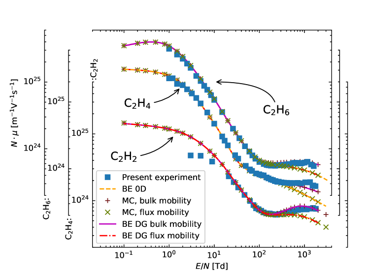
Figure 6: Mobility in C2H2, C2H4 and C2H6: present experiment and modelling results. The results and $N\mu$ scale for C2H4 and C2H6 have been shifted. ’Present experiment’ corresponds to the uncorrected experimental data. The corrected data are not shown here because of the small correction factors for the bulk drift velocity / mobility.

5.2 Diffusion tensor

The present experimental results for the gas number density times the longitudinal component of the diffusion tensor, $ND_{\rm L}$, for C2H2, C2H4 and C2H6 are given in A, table 3. They are shown in figure 7 together with previously measured data as well as with the kinetic computation values for the bulk longitudinal and transverse components of the diffusion tensor for each gas. The present measured values of $ND_{\rm L}$ exhibit larger scattering, which is explained by the higher uncertainty of the determination of $D_{\rm L}$ in the experiments ($\approx$10\text{\,}\mathrm{\char 37\relax}$$) compared to that of the drift velocity.

Above $100\text{\,}\mathrm{T}\mathrm{d}$ there is reasonable agreement of the present measurements with previous experimental data and the modelling results, for the three gases. Below $100\text{\,}\mathrm{T}\mathrm{d}$ however, the present measurements evidence the same qualitative behaviour but are systematically above previous measurements. Note that the application of the correction procedure, detailed in section 4, to our experimental results leads to much better agreement with previously measured data, in particular for C2H4 and C2H6.

The modelling results for $D_{\rm L}$ in C2H2 and C2H4 below $2\text{\,}\mathrm{T}\mathrm{d}$ and $5\text{\,}\mathrm{T}\mathrm{d}$, respectively, also deviate from all experimental results indicating that the corresponding cross section sets require improvement. In each of the three gases, the values of the transverse component of the diffusion tensor, $D_{\rm T}$, obtained by the kinetic computations, are very different from the longitudinal component, $D_{\rm L}$. The measurement of data of this component can provide additional tests for the fitting of the electron collision cross sections.

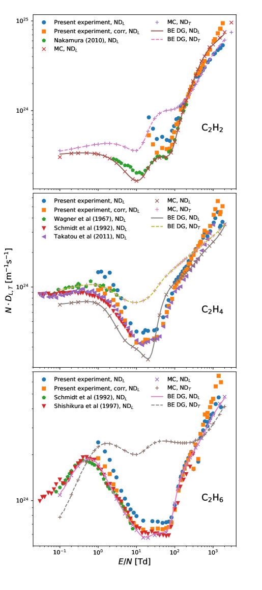
Figure 7: Longitudinal and transverse bulk components of the diffusion tensor in C2H2, C2H4 and C2H6. Experimental results: present experiment, Wagner et al [20], Schmidt and Roncossek [19], Shishikura et al [24], Nakamura [14], Takatou et al [18]. Modelling results: MC and BE DG ($ND_{\rm L}$ and $ND_{\rm T}$). The figures share the same $E/N$ scale. The panels show both the uncorrected and corrected experimental results of this study.

5.3 Effective ionization frequency and SST ionization coefficient

The experimental and modelling results for the reduced effective ionization frequency, $\nu_{\mathrm{eff}}/N$, for the three gases studied are displayed in figure 8. To our best knowledge this is the first report of $\nu_{\mathrm{eff}}$ in these three gases for an extended range of $$100\text{\,}\mathrm{T}\mathrm{d}$\leq E/N\leq$1790\text{\,}\mathrm{T}\mathrm{d}$$, for which the estimated experimental error of the data is $\leq$8\text{\,}\mathrm{\char 37\relax}$$. Our measured data are also listed in A, table 4. In order to accommodate the results on the same figure, all gases share a same $\nu_{\mathrm{eff}}/N$ axis but the $E/N$ scales for C2H4 and C2H2 have been shifted to the right.

Good agreement between our measured and calculated results is generally found for $E/N$ values larger than about $200\text{\,}\mathrm{T}\mathrm{d}$, indicating that the electron collision cross section sets for the three gases are reasonably well adapted to allow for an appropriate determination of the rate coefficients for ground state ionization. Certain differences are obvious for lower $E/N$ values. These differences seem to result from the measurement and/or, more likely, from the fitting procudure (see figure 4).

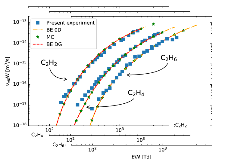
Figure 8: Reduced effective ionization frequency in C2H2, C2H4 and C2H6: present experiment and modelling results. The results and $E/N$ scale for C2H4 and C2H6 are shifted horizontally. ’Present experiment’ corresponds to the uncorrected data.

Our experimental data for the reduced effective SST ionization coefficient, $\alpha_{\mathrm{eff}}/N$, obtained using equation (2), are compared with previous measurements and the kinetic computation results in figure 9. As $\alpha_{\mathrm{eff}}$ is derived from the set of parameters $\{W,D_{\rm L},\nu_{\mathrm{eff}}\}$, these results have a higher uncertainty than $\nu_{\mathrm{eff}}$ with an estimated experimental error of $\leq$ $10\text{\,}\mathrm{\char 37\relax}$. Notice that the kinetic computation results using method BE SST do not include the approximations involved in equation (2), but are directly obtained by solving the electron Boltzmann equation at SST conditions according to (7). In this respect, their comparison with the BE DG and MC results can indicate the range of validity of equation (2) or (12). Our experimental results of $\alpha_{\mathrm{eff}}/N$ are compiled in A, table 5 as well.

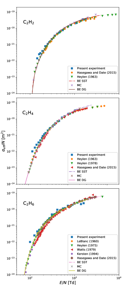
Figure 9: Reduced effective Townsend ionization coefficient in C2H2, C2H4 and C2H6. Experimental results: present experiment, Heylen [26, 29], Watts and Heylen [28], Kersten [25] and Hasegawa and Date [13]. Modelling results: BE SST, MC and BE DG. ’Present experiment’ corresponds to the uncorrected data.

Except for the low values of $E/N$, our results for the effective SST ionization coefficient are in excellent agreement with all previous results and the kinetic computations. At values close to the threshold, however, the present results are higher than previous measurements. Notice that Kersten’s effective Townsend ionization coefficient was measured under TOF conditions and corresponds to $\nu_{\mathrm{eff}}/W$ [25]. Thus, it represents the effective SST ionization coefficient $\alpha_{\mathrm{eff}}$ according to (2) only in the absence of diffusion, i.e., $D_{\rm L}=0$.

5.4 Effect of the vibrationally excited population

The cross sections sets used above were obtained considering only electron collisions with the ground state of the molecules. However, as polyatomic molecules have multiple vibrational modes and these modes can be degenerated, in these gases we can find a significant fraction of molecules in thermally excited vibrational states at room temperature. In addition to their contribution to energy losses due to elastic, exciting, ionizing and attaching collision processes, these excited states contribute to electron energy gains due to superelastic collisions and influence the EVDF and transport parameters, mainly at low to medium $E/N$ field values. The importance of their effect increases with the energy associated with the collision and the fractional population of thermally excited states with that energy. This population, however, decreases exponentially with energy. From the combination of these two factors, the effect on the EVDF should be maximum for a given energy value.

Taking into account the equations for the fractional populations and statistical weights of polyatomic molecules in B, we can estimate the populations of the different states of these gases.

Acetylene

has five vibrational modes, with the two bending modes ($v_{4}$ and $v_{5}$) double degenerated and with energies of, respectively, $0.075\text{\,}\mathrm{e}\mathrm{V}$ and $0.0905\text{\,}\mathrm{e}\mathrm{V}$ [47]. At a gas temperature of $293.15\text{\,}\mathrm{K}$, the vibrational states with fractional population above $0.1\text{\,}\mathrm{\char 37\relax}$ are indicated in table 1. At this temperature only around $85\text{\,}\mathrm{\char 37\relax}$ of the acetylene molecules are in the ground state and the vibrational population in excited states of modes $v_{4}$ and $v_{5}$ is significant.

Table 1: Fractional population of the first vibrational levels of C2H2 at $293.15\text{\,}\mathrm{K}$.

Vibr. state	short notation	g	Energy (eV)	Frac. pop. $(\%)$
(00000)	$v_{0}$	1	$0.0$	$85.37$
(10000)	$v_{1}$	1	$0.421$	$5.5\text{\times}{10}^{-6}$
(01000)	$v_{2}$	1	$0.245$	$5.3\text{\times}{10}^{-3}$
(00100)	$v_{3}$	1	$0.411$	$8.3\text{\times}{10}^{-6}$
(00010)	$v_{4}$	2	$0.075$	$8.47$
(00020)		3	$0.150$	$0.63$
(00001)	$v_{5}$	2	$0.0905$	$4.75$
(00002)		3	$0.180$	$0.20$
(00011)	$v_{4}+v_{5}$	4	$0.165$	$0.47$

Ethylene:

In contrast to C2H2, none of the twelve ethylene vibrational modes [47] is degenerated, where the lowest threshold energy for vibrational excitation to $v_{10}$ is $0.102\text{\,}\mathrm{e}\mathrm{V}$ and, at the same temperature, more than $95\text{\,}\mathrm{\char 37\relax}$ of the molecules are in the ground state.

Ethane:

All the degenerated vibrational modes of ethane [47] have energies above $0.15\text{\,}\mathrm{e}\mathrm{V}$ and at room temperature their fractional population is small. Overall, however, only $73\text{\,}\mathrm{\char 37\relax}$ of ethane molecules are in the ground state as mode $v_{4}$ has an excitation energy of only $0.036\text{\,}\mathrm{e}\mathrm{V}$. Molecules in the two first excited vibrational states of this mode represent $22\text{\,}\mathrm{\char 37\relax}$ of the total. On the other hand, as the excitation energy of the $v_{4}$ mode transitions is very small, the effect on the EVDF and transport parameters is also small.

Of the three gases analysed, the impact of the thermally excited vibrational population on the EVDF should be largest in C2H2. The vibrational excitation cross section set for C2H2 [39] is also more complete than the vibrational cross section sets for C2H4 and C2H6 used in this study. For these reasons we study the effect of the thermally excited vibrational states only for acetylene.

Our goal is to single out the contribution of the vibrationally excited molecules due to superelastic collisions and we will change the electron collision cross sections in such a way that, if we neglect these collisions, we obtain the same results as before. Starting from the recommended cross section set for ethylene [39], we introduce the following modifications:
a) We split the lumped cross sections for the vibrational excitation of modes $v_{1}/v_{3}$ and $v_{4}/v_{5}$ into individual cross sections for each modes, with a value of half of the original cross section. That is $\sigma_{v_{1}}=\sigma_{v_{3}}=\frac{1}{2}\sigma_{v_{1}/v_{3}}$ and $\sigma_{v_{4}}=\sigma_{v_{5}}=\frac{1}{2}\sigma_{v_{4}/v_{5}}$.
b) The threshold for the excitation of modes $v_{1}$ and $v_{3}$ and of modes $v_{4}$ and $v_{5}$ is set at the same value as before of, respectively, $0.411\text{\,}\mathrm{e}\mathrm{V}$ and $0.0905\text{\,}\mathrm{e}\mathrm{V}$.
c) We assume that all molecules are in one of the three states $(00000)$, $(00010)$ and $(00001)$, with the fractional population, $\delta$, of the last two states in thermal equilibrium with the gas and the ground state fraction given by $\delta_{00000}=(1-\delta_{00010}-\delta_{00001})$.
d) We consider the following vibrational excitation processes for electron collisions with the ground state $(00000)$:

$$\begin{array}[]{lcl}\ce{e}+\ce{C2H2}(00000)&\to&\ce{e}+\ce{C2H2}(10000)\\ \ce{e}+\ce{C2H2}(00000)&\to&\ce{e}+\ce{C2H2}(01000)\\ \ce{e}+\ce{C2H2}(00000)&\to&\ce{e}+\ce{C2H2}(00100)\\ \ce{e}+\ce{C2H2}(00000)&\leftrightarrow&\ce{e}+\ce{C2H2}(00010)\\ \ce{e}+\ce{C2H2}(00000)&\leftrightarrow&\ce{e}+\ce{C2H2}(00001)\\ \ce{e}+\ce{C2H2}(00000)&\leftrightarrow&\ce{e}+\ce{C2H2}(00011)\end{array}$$

where reactions with double-arrows include superelastic collisions.
f) We additionaly include the following vibrational excitation processes on collisions with states $(00010)$ and $(00001)$:

$$\begin{array}[]{lcl}\ce{e}+\ce{C2H2}(00010)&\to&\ce{e}+\ce{C2H2}(10010)\\ \ce{e}+\ce{C2H2}(00010)&\to&\ce{e}+\ce{C2H2}(01010)\\ \ce{e}+\ce{C2H2}(00010)&\to&\ce{e}+\ce{C2H2}(00110)\\ \ce{e}+\ce{C2H2}(00010)&\leftrightarrow&\ce{e}+\ce{C2H2}(00020)\\ \ce{e}+\ce{C2H2}(00010)&\leftrightarrow&\ce{e}+\ce{C2H2}(00011)\\ \ce{e}+\ce{C2H2}(00010)&\to&\ce{e}+\ce{C2H2}(00021)\end{array}$$

and

$$\begin{array}[]{lcl}\ce{e}+\ce{C2H2}(00001)&\to&\ce{e}+\ce{C2H2}(10001)\\ \ce{e}+\ce{C2H2}(00001)&\to&\ce{e}+\ce{C2H2}(01001)\\ \ce{e}+\ce{C2H2}(00001)&\to&\ce{e}+\ce{C2H2}(00101)\\ \ce{e}+\ce{C2H2}(00001)&\leftrightarrow&\ce{e}+\ce{C2H2}(00011)\\ \ce{e}+\ce{C2H2}(00001)&\leftrightarrow&\ce{e}+\ce{C2H2}(00002)\\ \ce{e}+\ce{C2H2}(00001)&\to&\ce{e}+\ce{C2H2}(00012)\end{array}$$

adopting for these processes the same cross sections as the corresponding excitations from the ground state.
e) We further assume that the electron collision cross sections for momentum transfer, electronic excitation, ionization and attachment with the vibrational states $(00010)$ and $(00001)$ are the same as for state $(00000)$.

Note that if we neglect superelastic collisions, the EVDF and swarm parameters obtained with these modified cross sections and electron collision reactions are exactly the same as with the original set [39] and are independent of the fractional population of levels $(00010)$ and $(00001)$.

The influence of superelastic collisions is ilustrated in figure 10 which shows the isotropic component $\hat{f}_{0}(\epsilon)$ of the EVDF as a function of the electron kinetic energy, $\epsilon=m_{\mathrm{e}}v^{2}/2$, calculated at $E/N$ values of $1\text{\,}\mathrm{T}\mathrm{d}10\text{\,}\mathrm{T}\mathrm{d}$, respectively, with and without the inclusion of superelastic processes. Pronounced differences between the corresponding isotropic distributions $\hat{f}_{0}(\epsilon)$ are found at $E/N=$1\text{\,}\mathrm{T}\mathrm{d}$$, while the impact of superelastic electron collision processes is comparatively small at $10\text{\,}\mathrm{T}\mathrm{d}$. This finding is not only reflected by the isotropic distribution but also by different macroscopic properties.

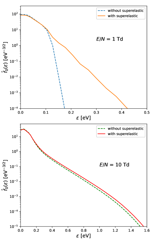
Figure 10: Isotropic component of the EVDF in C2H2 at $293.15\text{\,}\mathrm{K}$ for $1\text{\,}\mathrm{T}\mathrm{d}10\text{\,}\mathrm{T}\mathrm{d}$, with and without superelasic collision processes included.

The influence of superelastic collisions is mostly visible in the drift velocity and mobility as shown in figure 11. This figure compares the values of mobility and the longitudinal and transverse bulk components of the diffusion tensor obtained with the original cross sections set with the results obtained using the modified set with and without the inclusion of superelastic processes. As predicted, the results of the modified set neglecting superelastic collisions are the same as those obtained with the original set. Superelastic collisions are responsible for a reduction of the electron mobility in the range of low reduced field, visible up to approximately $20\text{\,}\mathrm{T}\mathrm{d}$. The influence on the components of the diffusion tensor is overall smaller than that on the mobility with the largest differences in the longitudinal component around $10\text{\,}\mathrm{T}\mathrm{d}$.

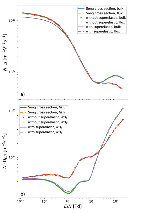
Figure 11: (a) Mobility and longitudinal and (b) transverse bulk components of the diffusion tensor in C2H2 at $293.15\text{\,}\mathrm{K}$: modelling results obtained with the electron collision cross sections from [39] without considering superelastic processes and with a modified set with and without superelastic processes.

As the impact of superelastic collisions decreases remarkably above about $20\text{\,}\mathrm{T}\mathrm{d}$, their influence on the effective ionization frequency and Townsend ionization coefficient is negligible.

6 Concluding remarks

We have investigated electron swarm parameters in C2H2, C2H4 and C2H6 experimentally using a scanning drift tube, as well as computationally by solutions of the electron Boltzmann equation and via Monte Carlo simulation, corresponding to both time-of-flight and steady-state Townsend conditions. The measured data made it possible to derive the bulk drift velocity, the bulk longitudinal component of the diffusion tensor and the effective ionization frequency of the electrons, for the wide range of the reduced electric field from 1 to $1790\text{\,}\mathrm{T}\mathrm{d}$. The measured TOF transport parameters as well as the effective SST ionization coefficient, deduced from the TOF swarm parameters, have been compared to experimental data obtained in previous studies. Here, generally good agreement with most of the transport parameters and the effective SST ionization coefficients obtained in these earlier studies was found. In the case of the drift velocity or the mobility, respectively, and the longitudinal component of the diffusion tensor we found disagreements at low or high values of $E/N$.

The experimental data have undergone a correction procedure, which was supposed to quantify the errors caused by the dependence of the sensitivity of the detector of the drift cell on the energy distribution of the electrons in the swarm that may have a spatial dependence.

In particular, in case of C2H2 our measured drift velocities at low $E/N$ agree well with previous data of Bowman and Gordon [16] but not with the results of Cottrell and Walker [17] as well as of Nakamura [14]. Further measurements in this range are required to clarify this contradiction.

The comparison of the experimental data was also carried out with swarm parameters resulting from various kinetic computations, which used the most recently recommended cross section sets [39, 40, 24]. Here, excellent agreement between electron Boltzmann equation and MC simulation results verifies the computational approaches and data for the three gases. The agreement of the computed data with the present and previously measured values of the reduced effective ionization frequency and SST ionization coefficient was generally good. However, certain differences between kinetic computational and measured results found for the drift velocities and, especially, for the longitudinal component of the diffusion tensor illustrate the need for an improvement of the existing collision cross section sets for the three hydrocarbon gases considered.

We have also studied the influence of the thermally excited vibrational populations on the transport parameters. In the case of C2H2 we have found that this population has a significant value and superelastic collisions influence the drift velocity and the components of the diffusion tensor up to $20\text{\,}\mathrm{T}\mathrm{d}$. The fitting of electron collision cross sections for this gas using swarm experiments should include these processes.

Appendix A Tables of experimental data

Table 2: Measured bulk drift velocity $W$ of electrons in C2H2, C2H4 and C2H6 at $293.15\text{\,}\mathrm{K}$. The exptl. values are the measured data while the cor. ones are corrected for systematic effects ($E/N$ in $\mathrm{T}\mathrm{d}$, $W$ in ${10}^{4}\text{\,}\mathrm{m}\mathrm{/}\mathrm{s}$).

$E/N$	$W$		$E/N$	$W$		$E/N$	$W$
	exptl.	cor.		exptl.	cor.		exptl.	cor.
C2H2
$3$	$1.43$	$1.43$	$125$	$8.36$	$8.33$	$450$	$29.6$	$30.3$
$5$	$2.36$	$2.35$	$145$	$9.38$	$9.35$	$480$	$31.9$	$32.7$
$9$	$3.48$	$3.47$	$160$	$10.1$	$10.2$	$540$	$36.0$	$37.1$
$21$	$4.88$	$4.86$	$170$	$10.8$	$10.9$	$600$	$40.4$	$41.7$
$27$	$5.14$	$5.12$	$190$	$11.9$	$11.9$	$720$	$50.2$	$52.2$
$34$	$5.38$	$5.36$	$220$	$13.6$	$13.7$	$830$	$58.4$	$61.0$
$47$	$5.75$	$5.72$	$230$	$14.0$	$14.2$	$1043$	$73.5$	$77.8$
$62$	$6.15$	$6.12$	$250$	$15.3$	$15.5$	$1120$	$77.9$	$82.8$
$74$	$6.37$	$6.35$	$270$	$16.8$	$17.0$	$1330$	$93.7$	$108$
$85$	$6.57$	$6.55$	$310$	$19.4$	$19.7$	$1530$	$108$	$117$
$96$	$7.17$	$7.15$	$360$	$23.0$	$23.4$	$1560$	$111$	$121$
$110$	$7.80$	$7.77$	$410$	$26.9$	$27.4$	$1790$	$122$	$135$
C2H4
$1$	$2.33$	$2.27$	$50$	$5.69$	$5.53$	$310$	$19.8$	$19.4$
$1.2$	$2.80$	$2.72$	$62$	$6.24$	$6.06$	$350$	$22.1$	$21.7$
$1.5$	$2.89$	$2.81$	$69$	$6.60$	$6.41$	$410$	$25.6$	$25.3$
$2$	$3.68$	$3.57$	$85$	$7.44$	$7.23$	$455$	$28.0$	$27.7$
$2.5$	$3.99$	$3.88$	$100$	$8.51$	$8.27$	$480$	$29.7$	$29.4$
$3.2$	$4.43$	$4.30$	$110$	$9.09$	$8.86$	$550$	$34.0$	$33.7$
$4$	$4.74$	$4.60$	$125$	$10.2$	$9.96$	$600$	$37.0$	$36.7$
$5$	$4.90$	$4.76$	$145$	$11.0$	$10.7$	$710$	$43.8$	$43.6$
$7$	$5.02$	$4.88$	$160$	$11.8$	$11.5$	$840$	$50.9$	$50.9$
$10$	$4.88$	$4.74$	$180$	$12.7$	$12.4$	$1040$	$64.7$	$65.2$
$15$	$4.70$	$4.57$	$200$	$13.9$	$13.5$	$1140$	$70.5$	$71.2$
$17$	$4.62$	$4.48$	$220$	$14.7$	$14.4$	$1330$	$82.6$	$83.9$
$20$	$4.61$	$4.48$	$230$	$15.3$	$15.0$	$1510$	$82.1$	$84.0$
$29$	$4.77$	$4.63$	$250$	$16.3$	$16.0$	$1570$	$86.1$	$88.3$
$34$	$4.96$	$4.82$	$270$	$17.6$	$17.3$	$1760$	$93.6$	$96.6$
C2H6
$1$	$3.23$	$3.14$	$48$	$5.36$	$5.22$	$350$	$20.3$	$20.1$
$1.5$	$3.97$	$3.86$	$60$	$5.55$	$5.42$	$410$	$24.0$	$23.9$
$2$	$4.58$	$4.45$	$70$	$5.68$	$5.55$	$470$	$27.8$	$27.7$
$2.5$	$4.84$	$4.71$	$82$	$5.93$	$5.80$	$550$	$33.3$	$33.4$
$3$	$5.02$	$4.88$	$100$	$6.46$	$6.32$	$610$	$37.3$	$37.6$
$4$	$5.06$	$4.93$	$125$	$7.52$	$7.36$	$710$	$43.2$	$43.7$
$5$	$5.31$	$5.17$	$145$	$8.44$	$8.28$	$715$	$42.4$	$43.0$
$6$	$5.39$	$5.25$	$160$	$9.18$	$9.01$	$836$	$49.3$	$50.3$
$7$	$5.49$	$5.34$	$180$	$10.2$	$10.0$	$900$	$53.8$	$55.0$
$8.5$	$5.53$	$5.38$	$200$	$11.3$	$11.1$	$1002$	$60.3$	$62.0$
$10$	$5.54$	$5.39$	$225$	$12.7$	$12.5$	$1170$	$71.8$	$74.5$
$15$	$5.45$	$5.30$	$250$	$14.3$	$14.1$	$1398$	$77.0$	$80.9$
$26$	$5.33$	$5.18$	$270$	$15.6$	$15.4$	$1606$	$82.9$	$88.1$
$36$	$5.31$	$5.17$	$310$	$17.7$	$17.5$

Table 3: Measured longitudinal component of the diffusion tensor times gas number density $D_{\rm L}N$ of electrons in C2H2, C2H4 and C2H6 at $293.15\text{\,}\mathrm{K}$. The exptl. values are the measured data while the cor. ones are corrected for systematic effects ($E/N$ in $\mathrm{T}\mathrm{d}$, $D_{\rm L}N$ in ${10}^{24}\text{\,}\mathrm{m}^{-1}\mathrm{s}^{-1}$).

$E/N$	$D_{\mathrm{L}}N$		$E/N$	$D_{\mathrm{L}}N$		$E/N$	$D_{\mathrm{L}}N$
	exptl.	cor.		exptl.	cor.		exptl.	cor.
C2H2
$21$	$0.84$	$0.53$	$160$	$1.10$	$1.02$	$480$	$2.68$	$3.00$
$27$	$0.63$	$0.42$	$170$	$1.17$	$1.10$	$540$	$2.82$	$3.24$
$34$	$0.48$	$0.34$	$190$	$1.31$	$1.28$	$600$	$3.03$	$3.75$
$47$	$0.51$	$0.38$	$220$	$1.44$	$1.43$	$720$	$3.46$	$4.28$
$62$	$0.47$	$0.37$	$230$	$1.53$	$1.53$	$830$	$3.70$	$4.78$
$74$	$0.46$	$0.38$	$250$	$1.67$	$1.68$	$1043$	$4.26$	$5.95$
$85$	$0.55$	$0.50$	$270$	$1.81$	$1.84$	$1120$	$4.36$	$6.25$
$96$	$0.67$	$0.57$	$310$	$1.97$	$2.04$	$1330$	$4.73$	$7.27$
$110$	$0.80$	$0.70$	$360$	$2.39$	$2.54$	$1530$	$4.98$	$8.14$
$125$	$0.83$	$0.74$	$410$	$2.39$	$2.59$	$1560$	$4.97$	$8.20$
$145$	$1.12$	$1.03$	$450$	$2.50$	$2.76$	$1790$	$5.35$	$9.43$
C2H4
$1$	$1.35$	$0.94$	$50$	$0.54$	$0.48$	$310$	$1.97$	$1.91$
$1.2$	$1.36$	$0.96$	$62$	$0.68$	$0.60$	$350$	$2.14$	$2.09$
$1.5$	$1.23$	$0.88$	$69$	$0.77$	$0.68$	$410$	$2.28$	$2.27$
$2$	$1.33$	$0.97$	$85$	$0.88$	$0.79$	$455$	$2.40$	$2.41$
$2.5$	$1.04$	$0.77$	$100$	$1.09$	$0.99$	$480$	$2.45$	$2.49$
$3.2$	$0.94$	$0.70$	$110$	$1.16$	$1.05$	$550$	$2.69$	$2.78$
$4$	$0.80$	$0.61$	$125$	$1.22$	$1.12$	$600$	$2.96$	$3.09$
$5$	$0.66$	$0.51$	$145$	$1.30$	$1.19$	$710$	$2.77$	$2.99$
$7$	$0.48$	$0.38$	$160$	$1.37$	$1.27$	$840$	$3.06$	$3.41$
$10$	$0.41$	$0.33$	$180$	$1.45$	$1.35$	$1040$	$3.64$	$4.26$
$15$	$0.40$	$0.33$	$200$	$1.51$	$1.41$	$1140$	$3.99$	$4.77$
$17$	$0.42$	$0.35$	$220$	$1.54$	$1.45$	$1330$	$4.49$	$5.61$
$20$	$0.42$	$0.35$	$230$	$1.68$	$1.59$	$1510$	$3.33$	$4.32$
$29$	$0.42$	$0.36$	$250$	$1.69$	$1.60$	$1570$	$3.43$	$4.51$
$34$	$0.43$	$0.37$	$270$	$1.85$	$1.77$	$1760$	$3.70$	$5.06$
C2H6
$1$	$2.41$	$1.89$	$48$	$0.71$	$0.65$	$350$	$2.29$	$2.33$
$1.5$	$2.10$	$1.68$	$60$	$0.72$	$0.66$	$410$	$1.80$	$1.87$
$2$	$1.85$	$1.49$	$70$	$0.73$	$0.67$	$470$	$2.58$	$2.74$
$2.5$	$1.57$	$1.28$	$82$	$0.78$	$0.72$	$550$	$2.89$	$3.15$
$3$	$1.42$	$1.17$	$100$	$0.94$	$0.87$	$610$	$3.31$	$3.67$
$4$	$1.16$	$0.96$	$125$	$1.24$	$1.17$	$710$	$3.08$	$3.53$
$5$	$1.03$	$0.86$	$145$	$1.44$	$1.36$	$715$	$3.28$	$3.76$
$6$	$0.94$	$0.79$	$160$	$1.55$	$1.48$	$836$	$3.45$	$4.10$
$7$	$0.88$	$0.74$	$180$	$1.69$	$1.62$	$900$	$3.66$	$4.43$
$8.5$	$0.83$	$0.71$	$200$	$1.79$	$1.73$	$1002$	$3.73$	$4.65$
$10$	$0.79$	$0.68$	$225$	$1.90$	$1.85$	$1170$	$4.30$	$5.61$
$15$	$0.74$	$0.64$	$250$	$2.01$	$1.98$	$1398$	$4.75$	$6.58$
$26$	$0.73$	$0.65$	$270$	$2.09$	$2.07$	$1606$	$4.10$	$5.98$
$36$	$0.73$	$0.65$	$310$	$1.61$	$1.62$

Table 4: Measured reduced effective ionization frequency $\nu_{\mathrm{eff}}/N$ of electrons in C2H2, C2H4 and C2H6 at $293.15\text{\,}\mathrm{K}$. The exptl. values are the measured data while the cor. ones are corrected for systematic effects ($E/N$ in $\mathrm{T}\mathrm{d}$, $\nu_{\mathrm{eff}}/N$ in ${10}^{-14}\text{\,}\mathrm{m}^{3}\mathrm{/}\mathrm{s}$).

$E/N$	$\nu_{\mathrm{eff}}/N$		$E/N$	$\nu_{\mathrm{eff}}/N$		$E/N$	$\nu_{\mathrm{eff}}/N$
	exptl.	cor.		exptl.	cor.		exptl.	cor.
C2H2
$145$	$0.001\,37$	$0.001\,36$	$310$	$0.0419$	$0.0422$	$830$	$0.853$	$0.879$
$160$	$0.002\,63$	$0.002\,64$	$360$	$0.0792$	$0.0800$	$1043$	$1.34$	$1.39$
$170$	$0.003\,25$	$0.003\,25$	$410$	$0.122$	$0.123$	$1120$	$1.50$	$1.56$
$190$	$0.004\,87$	$0.004\,88$	$450$	$0.158$	$0.161$	$1330$	$2.25$	$2.37$
$220$	$0.0109$	$0.0109$	$480$	$0.201$	$0.204$	$1530$	$3.06$	$3.25$
$230$	$0.0111$	$0.0111$	$540$	$0.263$	$0.268$	$1560$	$3.36$	$3.57$
$250$	$0.0171$	$0.0171$	$600$	$0.365$	$0.372$	$1790$	$3.80$	$4.07$
$270$	$0.0235$	$0.0237$	$720$	$0.603$	$0.619$
C2H4
$125$	$0.001\,06$	$0.001\,05$	$270$	$0.0241$	$0.0238$	$710$	$0.501$	$0.501$
$145$	$0.001\,94$	$0.001\,91$	$310$	$0.0388$	$0.0385$	$840$	$0.696$	$0.698$
$160$	$0.003\,10$	$0.003\,05$	$350$	$0.0592$	$0.0587$	$1040$	$1.20$	$1.21$
$180$	$0.004\,63$	$0.004\,58$	$410$	$0.0881$	$0.0876$	$1140$	$1.36$	$1.37$
$200$	$0.006\,82$	$0.006\,75$	$455$	$0.122$	$0.121$	$1330$	$1.83$	$1.85$
$220$	$0.0101$	$0.009\,99$	$480$	$0.153$	$0.152$	$1510$	$2.30$	$2.33$
$230$	$0.0138$	$0.0136$	$550$	$0.234$	$0.233$	$1570$	$2.54$	$2.59$
$250$	$0.0186$	$0.0184$	$600$	$0.265$	$0.265$	$1760$	$2.90$	$2.97$
C2H6
$100$	$0.000\,673$	$0.000\,675$	$270$	$0.0429$	$0.0430$	$715$	$0.571$	$0.581$
$125$	$0.001\,96$	$0.001\,97$	$310$	$0.0861$	$0.0863$	$836$	$0.776$	$0.792$
$145$	$0.003\,85$	$0.003\,86$	$350$	$0.0988$	$0.0991$	$900$	$0.929$	$0.949$
$160$	$0.005\,21$	$0.005\,22$	$410$	$0.221$	$0.222$	$1002$	$1.20$	$1.23$
$180$	$0.006\,67$	$0.006\,69$	$470$	$0.230$	$0.233$	$1170$	$1.61$	$1.65$
$200$	$0.0137$	$0.0137$	$550$	$0.356$	$0.361$	$1398$	$1.46$	$1.51$
$225$	$0.0214$	$0.0215$	$610$	$0.417$	$0.423$	$1606$	$1.82$	$1.89$
$250$	$0.0309$	$0.0310$	$710$	$0.657$	$0.669$

Table 5: Reduced effective SST ionization coefficient $\alpha_{\mathrm{eff}}/N$ of electrons in C2H2, C2H4 and C2H6 at $293.15\text{\,}\mathrm{K}$ calculated according to (2) using the measured values of $W$, $D_{\rm L}$ and $\nu_{\mathrm{eff}}$ ($E/N$ in $\mathrm{T}\mathrm{d}$, $\alpha_{\mathrm{eff}}/N$ in ${10}^{-20}\text{\,}{\mathrm{m}}^{2}$). The exptl. values are calculated with the measured data while the cor. ones are obtained with the values corrected for systematic effects.

$E/N$	$\alpha_{\mathrm{eff}}/N$		$E/N$	$\alpha_{\mathrm{eff}}/N$		$E/N$	$\alpha_{\mathrm{eff}}/N$
	exptl.	cor.		exptl.	cor.		exptl.	cor.
C2H2
$145$	$0.0146$	$0.0145$	$310$	$0.221$	$0.219$	$830$	$1.63$	$1.65$
$160$	$0.0260$	$0.0258$	$360$	$0.358$	$0.356$	$1043$	$2.08$	$2.15$
$170$	$0.0301$	$0.0299$	$410$	$0.473$	$0.470$	$1120$	$2.19$	$2.28$
$190$	$0.0413$	$0.0411$	$450$	$0.561$	$0.558$	$1330$	$2.80$	$3.00$
$220$	$0.0809$	$0.0805$	$480$	$0.667$	$0.663$	$1530$	$3.37$	$3.74$
$230$	$0.0796$	$0.0791$	$540$	$0.778$	$0.775$	$1560$	$3.61$	$4.07$
$250$	$0.113$	$0.112$	$600$	$0.974$	$0.973$	$1790$	$3.71$	$4.33$
$270$	$0.143$	$0.142$	$720$	$1.32$	$1.33$
C2H4
$125$	$0.0104$	$0.0105$	$270$	$0.138$	$0.140$	$710$	$1.24$	$1.26$
$145$	$0.0177$	$0.0178$	$310$	$0.200$	$0.202$	$840$	$1.50$	$1.53$
$160$	$0.0264$	$0.0267$	$350$	$0.275$	$0.278$	$1040$	$2.10$	$2.16$
$180$	$0.0366$	$0.0370$	$410$	$0.355$	$0.358$	$1140$	$2.21$	$2.28$
$200$	$0.0495$	$0.0500$	$455$	$0.453$	$0.457$	$1330$	$2.57$	$2.69$
$220$	$0.0690$	$0.0698$	$480$	$0.539$	$0.544$	$1510$	$3.21$	$3.36$
$230$	$0.0905$	$0.0915$	$550$	$0.730$	$0.738$	$1570$	$3.41$	$3.59$
$250$	$0.115$	$0.117$	$600$	$0.765$	$0.772$	$1760$	$3.62$	$3.85$
C2H6
$100$	$0.0104$	$0.0107$	$270$	$0.286$	$0.291$	$715$	$1.52$	$1.57$
$125$	$0.0262$	$0.0268$	$310$	$0.511$	$0.519$	$836$	$1.80$	$1.86$
$145$	$0.0460$	$0.0470$	$350$	$0.518$	$0.524$	$900$	$2.00$	$2.07$
$160$	$0.0573$	$0.0585$	$410$	$0.994$	$1.01$	$1002$	$2.32$	$2.42$
$180$	$0.0662$	$0.0675$	$470$	$0.906$	$0.925$	$1170$	$2.68$	$2.82$
$200$	$0.123$	$0.126$	$550$	$1.19$	$1.22$	$1398$	$2.20$	$2.29$
$225$	$0.173$	$0.177$	$610$	$1.26$	$1.29$	$1606$	$2.50$	$2.60$
$250$	$0.223$	$0.227$	$710$	$1.74$	$1.79$

Appendix B Statistical weights and statistical sums

The fractional populations for the levels of a polyatomic molecule with $n_{v}$ modes and vibrational quantum numbers $(v_{1}v_{2}v_{3}\ldots)$ are given by

$$\delta_{(v_{1}v_{2}v_{3}\ldots)}=\frac{g_{(v_{1}v_{2}v_{3}\ldots)}}{Q_{v}}\exp\left(-\frac{\epsilon_{(v_{1}v_{2}v_{3}\ldots)}}{k_{B}T}\right)$$ (20)

where $\epsilon_{(v_{1}v_{2}v_{3}\ldots)}$ is the level energy and $g$ the total statistical weight,

$$g_{(v_{1}v_{2}v_{3}\ldots)}=\prod_{n=1}^{n=n_{v}}\frac{(v_{n}+d_{n}-1)!}{v_{n}!(d_{n}-1)!}$$ (21)

where $d_{n}$ is the degeneracy multiplicity for mode $n$, and $Q_{v}$ the vibrational statistical sum which, in the harmonic oscilator approximation for the vibrational states, is

$$Q_{v}=\prod_{n=1}^{n=n_{v}}(1-Z_{n})^{-d_{n}}\,,\quad Z_{n}=\exp\{-hc\nu_{n}/k_{B}T\}$$ (22)

where $\nu_{n}$ are the vibrational frequencies.

References

References

- [1] Adamovich I V and Lempert W R 2014 Plasma Physics and Controlled Fusion 57 014001 doi: 10.1088/0741-3335/57/1/014001
- [2] Starikovskiy A and Aleksandrov N 2013 Progress in Energy and Combustion Science 39 61 – 110 ISSN 0360-1285 doi: 10.1016/j.pecs.2012.05.003
- [3] Kosarev I, Aleksandrov N, Kindysheva S, Starikovskaia l S and Starikovskii A Y 2009 Combustion and flame 156 221–233
- [4] Kosarev I, Pakhomov A, Kindysheva S, Anokhin E and Aleksandrov N 2013 Plasma Sources Science and Technology 22 045018
- [5] Kosarev I, Kindysheva S, Aleksandrov N and Starikovskiy A Y 2015 Combustion and Flame 162 50–59
- [6] Kosarev I, Kindysheva S, Momot R, Plastinin E, Aleksandrov N and Starikovskiy A Y 2016 Combustion and Flame 165 259–271
- [7] Robertson J 2002 Materials Science and Engineering: R: Reports 37 129 – 281 ISSN 0927-796X doi: 10.1016/S0927-796X(02)00005-0
- [8] Kumar M and Ando Y 2010 Journal of Nanoscience and Nanotechnology 10 3739–3758 ISSN 1533-4880 doi: 10.1166/jnn.2010.2939
- [9] Fonte P and Peskov V 2010 Plasma Sources Science and Technology 19 034021 doi: 10.1088/0963-0252/19/3/034021
- [10] von Keudell A, Schwarz-Selinger T, Jacob W and Stevens A 2001 Journal of Nuclear Materials 290-293 231 – 237 ISSN 0022-3115 14th Int. Conf. on Plasma-Surface Interactions in Controlled Fusion Devices
- [11] Varanasi P, Giver L and Valero F 1983 Journal of Quantitative Spectroscopy and Radiative Transfer 30 497 – 504 ISSN 0022-4073 doi: 10.1016/0022-4073(83)90003-1
- [12] Courtin R, Gautier D, Marten A, Bezard B and Hanel R 1984 Astrophysical Journal 287 899–916 doi: 10.1086/162748
- [13] Hasegawa H and Date H 2015 Journal of Applied Physics 117 133302 doi: 10.1063/1.4916606
- [14] Nakamura Y 2010 Journal of Physics D: Applied Physics 43 365201 doi: 10.1088/0022-3727/43/36/365201
- [15] Cottrell T L, Pollock W J and Walker I C 1968 Trans. Faraday Soc. 64(0) 2260–2266 doi: 10.1039/TF9686402260
- [16] Bowman C R and Gordon D E 1967 The Journal of Chemical Physics 46 1878–1883 doi: 10.1063/1.1840948
- [17] Cottrell T L and Walker I C 1965 Trans. Faraday Soc. 61(0) 1585–1593 doi: 10.1039/TF9656101585
- [18] Takatou J, Sato H and Nakamura Y 2011 Journal of Physics D: Applied Physics 44 315201 doi: 10.1088/0022-3727/44/31/315201
- [19] Schmidt B and Roncossek M 1992 Australian Journal of Physics 45 351–364 doi: 10.1071/PH920351
- [20] Wagner E B, Davis F J and Hurst G S 1967 The Journal of Chemical Physics 47 3138–3147 doi: 10.1063/1.1712365
- [21] Christophorou L G, Hurst G S and Hadjiantoniou A 1966 The Journal of Chemical Physics 44 3506–3513 doi: 10.1063/1.1727257
- [22] Hurst G S, O’Kelly L B, Wagner E B and Stockdale J A 1963 The Journal of Chemical Physics 39 1341–1345 doi: 10.1063/1.1734438
- [23] Bortner T E, Hurst G S and Stone W G 1957 Review of Scientific Instruments 28 103–108 doi: 10.1063/1.1715825
- [24] Shishikura Y, Asano K and Nakamura Y 1997 Journal of Physics D: Applied Physics 30 1610–1615 doi: 10.1088/0022-3727/30/11/010
- [25] Kersten H J 1994 Messung der Driftgeschwindigkeit und des effektiven Townsendkoeffizienten von Elektronen bei hohen elektrischen Feldstärken Diploma thesis Ruprecht-Karls-Universität Heidelberg
- [26] Heylen A E D 1963 The Journal of Chemical Physics 38 765–771 doi: 10.1063/1.1733735
- [27] Heylen A E D 1978 International Journal of Electronics 44 367–374 doi: 10.1080/00207217808900831
- [28] Watts M P and Heylen A E D 1979 Journal of Physics D: Applied Physics 12 695–702 doi: 10.1088/0022-3727/12/5/010
- [29] Heylen A E D 1975 International Journal of Electronics 39 653–660 doi: 10.1080/00207217508920532
- [30] LeBlanc O H and Devins J C 1960 Nature 188 219–220 doi: 10.1038/188219a0
- [31] Blevin H A and Fletcher J 1984 Aust. J. Phys. 37 593–600 doi: 10.1071/PH840593
- [32] Donkó Z, Hartmann P, Korolov I, Jeges V, Bošnjaković D and Dujko S 2019 Plasma Sources Science and Technology 28 095007 doi: 10.1088/1361-6595/ab3a58
- [33] Ramo S 1939 Proc. IRE 27 584
- [34] Korolov I, Vass M, Bastykova N K and Donkó Z 2016 Review of Scientific Instruments 87 063102 doi: 10.1063/1.4952747
- [35] Korolov I, Vass M and Donkó Z 2016 Journal of Physics D: Applied Physics 49 415203 doi: 10.1088/0022-3727/49/41/415203
- [36] Vass M, Korolov I, Loffhagen D, Pinhão N and Donkó Z 2017 Plasma Sources Science and Technology 26 065007 doi: 10.1088/1361-6595/aa6789
- [37] Shockley W 1938 J. Appl. Phys. 9 635
- [38] Sirkis M and Holonyak N 1966 Am. J. Phys. 34 943
- [39] Song M Y, Yoon J S, Cho H, Karwasz G P, Kokoouline V, Nakamura Y and Tennyson J 2017 Journal of Physical and Chemical Reference Data 46 013106 doi: 10.1063/1.4976569
- [40] Fresnet F, Pasquiers S, Postel C and Puech V 2002 Journal of Physics D: Applied Physics 35 882–890 doi: 10.1088/0022-3727/35/9/308
- [41] Leyh H, Loffhagen D and Winkler R 1998 Computer Physics Communications 113 33 – 48 ISSN 0010-4655 doi: 10.1016/S0010-4655(98)00062-9
- [42] Kumar K, Skullerud H and Robson R 1980 Aust. J. Phys. 33 343–448 doi: 10.1071/PH800343b
- [43] Segur P, Bordage M C, Balaguer J P and Yousfi M 1983 J. Comput. Phys. 50 116–37
- [44] Dujko S, White R D, Petrović Z L and Robson R E 2010 Phys. Rev. E 81(4) 046403 doi: 10.1103/PhysRevE.81.046403
- [45] Dujko S, White R D, Petrović Z L and Robson R E 2011 Plasma Sources Science and Technology 20 024013 doi: 10.1088/0963-0252/20/2/024013
- [46] Kondo K and Tagashira H 1990 Journal of Physics D: Applied Physics 23 1175–1183 doi: 10.1088/0022-3727/23/9/007
- [47] Shimanouchi T 1972 Tables of Molecular Vibrational Frequencies Consolidated Volume I Report NSDRS-NBS 39 National Bureau of Standards, Washington