Resonant field enhancement near bound states in the continuum on periodic structures

Abstract

On periodic structures sandwiched between two homogeneous media, a bound state in the continuum (BIC) is a guided Bloch mode with a frequency within the radiation continuum. BICs are useful, since they give rise to high quality-factor ($Q$-factor) resonances that enhance local fields for diffraction problems with given incident waves. For any BIC on a periodic structure, there is always a surrounding family of resonant modes with $Q$-factors approaching infinity. We analyze field enhancement around BICs using analytic and numerical methods. Based on a perturbation method, we show that field enhancement is proportional to the square-root of the $Q$-factor, and it depends on the adjoint resonant mode and its coupling efficiency with incident waves. Numerical results are presented to show different asymptotic relations between the field enhancement and the Bloch wavevector for different BICs. Our study provides a useful guideline for applications relying on resonant enhancement of local fields.

I Introduction

Bound states in the continuum (BICs) for photonic systems are attracting significant research interest mainly because they lead to resonances of extremely high quality factors ($Q$-factors) hsu16 ; kosh19 . A BIC is a trapped or guided mode with a frequency in the radiation continuum where radiative waves can propagate to or from infinity neumann29 , and it can only exist on a lossless structure that is infinite in at least one spatial direction. Many recent works are concerned with BICs on periodic structures (with one or two periodic directions) sandwiched between two homogeneous media bonnet94 ; padd00 ; tikh02 ; shipman03 ; port05 ; shipman07 ; mari08 ; lee12 ; hsu13_2 ; bulg14b ; yang14 ; zhen14 ; hu15 ; gao16 ; gan16 ; li16 ; ni16 ; yuan17 ; bulg17pra ; hu18 ; doel18 ; zhang18 . On such a periodic structure, a BIC is a Bloch mode that decays exponentially in the surrounding homogeneous media, but unlike ordinary guided modes below the lightline, it co-exists with plane waves above the lightline. These plane waves have the same frequency and wavevector as the BIC, and can propagate to or from infinity in the surrounding media. Importantly, a BIC can be regarded as a resonant mode with an infinite $Q$-factor hsu13_2 . When the structure is perturbed slightly, a BIC usually (but not always) becomes a resonant mode with a large $Q$-factor yuan17_4 ; kosh18 ; lijun19pr . On periodic structures, a BIC is surrounded by resonant modes that depend on the Bloch vector continuously. The $Q$-factors of these resonant modes tend to infinity as the Bloch wavevector approaches that of the BIC hsu13_2 . The relation between the $Q$-factor and the Bloch wavevector has been analyzed in a number of papers lijun17pra ; lijun18pra ; jin19 ; lijun19pr .

Strong local fields induced by high-$Q$ resonances are essential to applications such as lasing kodi17 and sensing romano19 ; yesi19 , and can be used enhance emissive processes and and nonlinear effects lijun16pra ; lijun17pra ; lijun19siam . For lossless dielectric structures, the $Q$-factor (denoted by $Q$) of a resonant mode accounts for radiation losses only, and the field enhancement, defined as the ratio of the maximum amplitudes of the total and incident waves, is known to be proportional to $\sqrt{Q}$. Therefore, using the asymptotic relations between the $Q$-factors and the wavevectors, the field enhancement caused by a high-$Q$ resonance near a BIC is known qualitatively shipman05 ; mocella15 ; yoon15 . In this paper, we use a perturbation method to derive a rigorous formula for field enhancement and perform a detailed numerical study for field enhancement around a few BICs with distinct asymptotic behavior. The perturbation theory is developed for two-dimensional (2D) periodic structures with one periodic direction (i.e., 1D periodicity). The formula reveals not only the square-root dependence on the $Q$-factor, but also the relevance of adjoint resonant modes and their coupling efficiency with incident waves. The numerical examples are carried out for a few BICs for which the corresponding $Q$-factors have different asymptotic behaviors.

The rest of this paper is organized as follows. In Sec. II, we briefly recall the definitions and properties of BICs and resonant modes on 2D periodic structures, and establish a useful formula for the $Q$-factor. In Sec. III, we derive a formula for field enhancement using a perturbation method. Numerical examples for four BICs with very different properties are presented in Sec. IV. The paper is concluded with a brief discussion in Sec. V.

II Resonant modes around BICs

Many recent studies on photonic BICs are concerned with dielectric periodic structures. Two-dimensional periodic structures that are uniform in one spatial direction and periodic in another direction are relatively simple to analyze theoretically, but they still capture the nontrivial physics involving the BICs bonnet94 ; shipman03 ; port05 ; shipman07 ; mari08 ; bulg14b ; hu15 ; yuan17 ; hu18 . We consider 2D periodic structures that are invariant in $z$, periodic in $y$ with period $L$, and sandwiched between two homogeneous media given in $x<-D$ and $x>D$ for a positive $D$, respectively. Let ${\bf r}=(x,y)$ and $\epsilon=\epsilon({\bm{r}})$ be the dielectric function for such a periodic structure and the surrounding media, then $\epsilon$ is real and positive, and

$$\epsilon(x,y+L)=\epsilon({\bm{r}})$$ (1)

for all ${\bm{r}}$. For simplicity, we assume the surrounding medium is vacuum, thus

$$\epsilon({\bm{r}})=1,\quad\mbox{if}\ |x|>D.$$ (2)

For the $E$-polarization and a time harmonic field with the time dependence $e^{-i\omega t}$ ($\omega$ is the angular frequency), the $z$ component of the electric field, denoted as $E_{z}$ or $u$, satisfies the following 2D Helmholtz equation

$$\partial_{x}^{2}u+\partial_{y}^{2}u+k^{2}\epsilon({\bm{r}})u=0,$$ (3)

where $k=\omega/c$ is the freespace wavenumber and $c$ is the speed of light in vacuum.

A BIC on the periodic structure is a solution of Eq. (3) for a real $\omega>0$, given in the form of a Bloch mode

$$u({\bm{r}})=\phi({\bm{r}})e^{i\beta y},$$ (4)

where $\phi$ is periodic in $y$ with period $L$, $\phi\to 0$ exponentially as $|x|\to\infty$, $\beta$ is the real Bloch wavenumber, and $k>|\beta|$. Due to the periodicity in $y$, $\beta$ can be restricted by $|\beta|\leq\pi/L$. If $\beta=0$, the BIC is a standing wave, otherwise, it is a propagating BIC. Since the lightlines (in the $\beta$-$k$ plane) are defined as $k=\pm\beta$, a BIC is a guided mode above the lightline. For $|x|>D$, any Bloch mode given by Eq. (4) can be expanded in plane waves as

$$u({\bm{r}})=\sum_{m=-\infty}^{\infty}c_{m}^{\pm}e^{i[\beta_{m}y\pm\alpha_{m}(x\mp D)]},\quad\pm x>D,$$ (5)

where $\beta_{0}=\beta$, and

$$\beta_{m}=\beta+\frac{2\pi m}{L},\quad\alpha_{m}=\sqrt{k^{2}-\beta_{m}^{2}}.$$ (6)

Most (but not all) BICs are found for $k$ satisfying

$$|\beta|<k<\frac{2\pi}{L}-|\beta|.$$ (7)

In that case, all $\alpha_{m}$ for $m\neq 0$ are pure imaginary with positive imaginary parts, and only $\alpha_{0}$ is real. Since a BIC must decay exponentially as $|x|\to\infty$, if condition (7) is satisfied, then we must have $c_{0}^{+}=c_{0}^{-}=0$.

A resonant mode (also called resonant state, quasi-normal mode, guided resonance, or scattering resonance) on the periodic structure is a solution of Eq. (3) that radiates power outwards as $|x|\to\infty$ fan02 ; amgad19 . Since $\epsilon$ is real and energy is conserved, the frequency $\omega$ of a resonant mode must have a negative imaginary part, so that it can decay with time as it radiates power to infinity. The $Q$-factor of a resonant mode can be defined as $Q=-0.5\mbox{Re}(\omega)/\mbox{Im}(\omega)$. Expansion (5) is still valid, provided that all $\alpha_{m}=\sqrt{k^{2}-\beta_{m}^{2}}$ are properly defined to maintain continuity as $\mbox{Im}(\omega)$ tends to zero. This can be achieved by choosing the negative imaginary axis (instead of the negative real axis) as the branch cut for the complex square root. More precisely, if $\eta=|\eta|e^{i\theta}$ for $-\pi/2<\theta\leq 3\pi/2$ (instead of $-\pi<\theta\leq\pi$), then $\sqrt{\eta}=\sqrt{|\eta|}e^{i\theta/2}$. If $\mbox{Re}(k)$ satisfies condition (7) and $\mbox{Im}(k)$ is small, then all $\alpha_{m}$ for $m\neq 0$ have positive imaginary parts, and $\alpha_{0}$ has a positive real part and a small negative imaginary part. In that case, the plane wave $\exp[i(\beta y+\alpha_{0}x)]$ radiates power in the positive $x$ direction and blows up as $x\to+\infty$. The coefficients $c_{0}^{\pm}$ of a resonant mode should be nonzero. The resonant modes form bands with complex frequency $\omega$ depending on real Bloch wavenumber $\beta$. A BIC corresponds to a special point on the dispersion curve of a band of resonant modes, where $\omega$ becomes real. Therefore, a BIC can be regarded as special resonant mode with an infinite $Q$-factor.

Let $\omega_{\circ}$ and $\beta_{\circ}$ be the frequency and Bloch wavenumber of a BIC respectively, and $\omega$ be the complex frequency of a resonant mode near the BIC for a $\beta$ near $\beta_{\circ}$. Perturbation theories provide approximate formulas for $\omega$ and the $Q$-factor assuming $|\beta-\beta_{\circ}|$ is small. In general, we have

$$\mbox{Re}(\omega)-\omega_{\circ}\sim\beta-\beta_{\circ},$$ (8)

$$\mbox{Im}(\omega)\sim(\beta-\beta_{\circ})^{2},$$ (9)

$$Q\sim 1/|\beta-\beta_{\circ}|^{2}.$$ (10)

Special results have been derived for standing waves on periodic structures with a reflection symmetry in the periodic direction lijun17pra ; lijun18pra ; lijun19pr . Assuming the periodic structure is symmetric in $y$ (i.e., $\epsilon$ is even in $y$), a standing wave is either symmetric in $y$ (even in $y$) or antisymmetric in $y$ (odd in $y$). For both cases, it is known that

$$\mbox{Re}(\omega)-\omega_{\circ}\sim\beta^{2}.$$ (11)

Moreover, for a symmetric standing wave, we have

$$\mbox{Im}(\omega)\sim\beta^{4}.$$ (12)

For a typical antisymmetric standing wave, Eq. (9), i.e., $\mbox{Im}(\omega)\sim\beta^{2}$, is valid, but under special conditions, $\mbox{Im}(\omega)$ satisfies

$$\mbox{Im}(\omega)\sim\beta^{6}.$$ (13)

Therefore, depending on the nature of the standing wave, the $Q$-factor follows different scaling laws, i.e., $1/\beta^{2}$, $1/\beta^{4}$, or $1/\beta^{6}$.

The $Q$-factor of a resonant mode is often defined as the ratio between the energy stored in a cavity and the power loss, multiplied by the resonant frequency (real part of the complex frequency). For our 2D periodic structure, the cavity can be chosen as the rectangle

$$\Omega=\{(x,y)\,:\,|x|<D,\,|y|<L/2\}.$$ (14)

In Appendix A, we derive a formula for the $Q$-factor, i.e., Eq. (16) below, based on a wave-field splitting outside the cavity. If there is only one radiation channel, i.e., $\alpha_{0}$ is in the fourth quadrant close to the positive real axis, and all $\alpha_{m}$ for $m\neq 0$ are in the second quadrant close to the positive imaginary axis, then, the wave field outside the cavity can be written as

$$u({\bm{r}})=u_{p}({\bm{r}})+u_{e}({\bm{r}}),\quad|x|>D,$$ (15)

where $u_{p}$ is the term for $m=0$ in the right hand side of Eq. (5) and $u_{e}$ is the sum of all other terms for $m\neq 0$. In that case, the $Q$-factor satisfies

$$\frac{1}{Q}=\frac{L\mbox{Re}(\alpha_{0})}{[\mbox{Re}(k)]^{2}}\cdot\frac{|c_{0}^{+}|^{2}+|c_{0}^{-}|^{2}}{\int_{\Omega}\epsilon|u|^{2}d{\bm{r}}+\int_{\Omega_{e}}|u_{e}|^{2}d{\bm{r}}},$$ (16)

where $\Omega_{e}$ is the union of two semi-infinite strips given by $|x|>D$ and $|y|<L/2$. The first and second integrals in the denominator are proportional to the electric energy stored in the cavity and the electric energy of the evanescent field $u_{e}$ outside the cavity. The numerator is proportional to the power radiated out by the plane wave $u_{p}$. Assuming the resonant mode is scaled such that

$$\max_{{\bm{r}}\in\Omega}|u({\bm{r}})|=1,$$ (17)

then $c_{0}^{+}$ and $c_{0}^{-}$ are dimensionless quantities, and Eq. (16) gives rise to

$$|c_{0}^{+}|^{2}+|c_{0}^{-}|^{2}\sim\frac{1}{Q}.$$ (18)

By reciprocity, corresponding to one resonant mode $u$ with a real Bloch wavenumber $\beta$ and a complex frequency $\omega$, there is another resonant mode (the adjoint resonant mode) $v$ with Bloch wavenumber $-\beta$ and the same complex frequency. We write $v$ as

$$v({\bm{r}})=\psi({\bm{r}})e^{-i\beta y},$$ (19)

and expand $v$ as

$$v({\bm{r}})=\sum_{m=-\infty}^{\infty}d_{m}^{\pm}e^{i[-\beta_{m}y\pm\alpha_{m}(x\mp D)]},\quad\pm x>D.$$ (20)

Apparently, Eq. (16) remains valid when $u$, $u_{e}$, $c_{0}^{\pm}$ are replaced by $v$, $v_{e}$ (similarly defined as $u_{e}$) and $d_{0}^{\pm}$. If we scale $v$ such that $\max_{(x,y)\in\Omega}|v(x,y)|=1$, then

$$|d_{0}^{+}|^{2}+|d_{0}^{-}|^{2}\sim\frac{1}{Q}.$$ (21)

III Field enhancement

In this section, we analyze the resonant effect of field enhancement by a perturbation method. For a 2D periodic structure given by a real dielectric function $\epsilon(x,y)$, we assume there is a resonant mode with a complex frequency $\omega_{*}$ and real Bloch wavenumber $\beta$. To avoid confusion with the diffraction solution excited by incident waves, we denote the resonant mode by $u_{*}$, its freespace wavenumber by $k_{*}$, define $\alpha_{m}^{*}$ by $\alpha_{m}^{*}=\sqrt{k_{*}^{2}-\beta_{m}^{2}}$, but still denote the expansion coefficients of $u_{*}$ [as in Eq. (5)] by $c_{m}^{\pm}$. The adjoint resonant mode is $v_{*}$, and its expansion coefficients are $d_{m}^{\pm}$.

We consider a diffraction problem for incident waves with a real frequency $\omega$ near (or exactly at) the real part of $\omega_{*}$. Two incident plane waves are given in the left ($x<-D$) and right ($x>D$) of the periodic structure, respectively, and their amplitudes $a_{0}^{+}$ and $a_{0}^{-}$ are assumed to satisfy

$$|a_{0}^{+}|^{2}+|a_{0}^{-}|^{2}=1.$$ (22)

Since two incident waves are involved, we choose to normalize them to fix the total incident power. In the left and right homogeneous media, the total field can be written as

$$u({\bm{r}})=a_{0}^{\pm}e^{i[\beta y\mp\alpha_{0}(x\mp D)]}$$ (23)

$$+\sum_{m=-\infty}^{\infty}b_{m}^{\pm}e^{i[\beta_{m}y\pm\alpha_{m}(x\mp D)]},\quad\pm x\geq D,$$ (24)

where $\alpha_{m}$ is defined in Eq. (6), and $b_{m}^{\pm}$ are the amplitudes of the outgoing plane waves. The wavevectors of the incident waves are $(\pm\alpha_{0},\beta)$. Notice that the resonant mode $u_{*}$ and the diffraction solution $u$ follow the same real Bloch wavenumber $\beta$. Again, we assume condition (7) is satisfied, then only $\alpha_{0}$ is real positive and all $\alpha_{m}$ for $m\neq 0$ are pure imaginary with positive imaginary parts.

To develop the perturbation theory, it is useful to write down the exact boundary conditions at $x=\pm D$ bao95 . Let $B$ be a linear operator acting on quasi-periodic functions of $y$, such that

$$Be^{i\beta_{m}y}=i\alpha_{m}e^{i\beta_{m}y}$$ (25)

for all integer $m$, then $u$ satisfies the following boundary conditions

$$\pm\frac{\partial u}{\partial x}=Bu-2i\alpha_{0}a_{0}^{\pm}e^{i\beta y},\quad x=\pm D.$$ (26)

For the complex frequency $\omega_{*}$, if we define a linear operator $B_{*}$ as in Eq. (25), with $\alpha_{m}$ replaced by $\alpha^{*}_{m}$, then the resonant mode $u_{*}$ satisfies

$$\pm\frac{\partial u_{*}}{\partial x}=B_{*}u_{*},\quad x=\pm D.$$ (27)

If $\delta=k-k_{*}$ is small (more precisely, $|\delta/k_{*}|$ is small), we try to find the diffraction solution $u$ by the following expansion:

$$u=\frac{C}{\delta}u_{*}+u_{0}+\delta u_{1}+\delta^{2}u_{2}+\cdots$$ (28)

The operator $B$ must also be expanded:

$$B=B_{*}+\delta B_{1}+\delta^{2}B_{2}+\cdots$$ (29)

It is easy to see that

$$\alpha_{m}=\sqrt{k_{*}^{2}-\beta_{m}^{2}+k^{2}-k_{*}^{2}}=\alpha^{*}_{m}+\frac{k_{*}}{\alpha^{*}_{m}}\delta+\cdots$$

Therefore, $B_{1}$ is a linear operator satisfying

$$B_{1}e^{i\beta_{m}y}=\frac{ik_{*}}{\alpha^{*}_{m}}e^{i\beta_{m}y}$$ (30)

for all integer $m$.

Inserting the expansions for $u$ and $B$ into Eq. (3) and boundary condition (26), we collect equations and boundary conditions at different powers of $\delta$. At $O(1/\delta)$, we simply get the Helmholtz equation and boundary conditions for $u_{*}$. At $O(1)$, we obtain the following inhomogeneous Helmholtz equation

$$\partial_{x}^{2}u_{0}+\partial_{y}^{2}u_{0}+k_{*}^{2}\epsilon u_{0}=-2Ck_{*}\epsilon u_{*}$$ (31)

and boundary conditions

$$\pm\frac{\partial u_{0}}{\partial x}-B_{*}u_{0}=CB_{1}u_{*}-2i\alpha_{0}^{*}a_{0}^{\pm}e^{i\beta y},\quad x=\pm D.$$ (32)

Multiplying Eq. (31) by $v_{*}$ and integrating on $\Omega$, we get

$$C=\frac{iL\alpha_{0}^{*}\,(a_{0}^{+}d_{0}^{+}+a_{0}^{-}d_{0}^{-})}{k_{*}R}$$ (33)

where

$$R=\int_{\Omega}\epsilon v_{*}u_{*}d{\bm{r}}+\frac{iL}{2}\sum_{m=-\infty}^{\infty}\frac{c_{m}^{+}d_{m}^{+}+c_{m}^{-}d_{m}^{-}}{\alpha^{*}_{m}}.$$

Additional details are given in Appendix B.

Field enhancement is often defined as the ratio of the amplitudes of the total and incident waves. Since the incident waves are normalized according to Eq. (22), $u_{*}$ is scaled to satisfy Eq. (17), and $|\delta/k_{*}|$ is supposed to be small, the amplitude of $u$, and also the field enhancement, can be approximated by $|C/\delta|$. The term $a_{0}^{+}d_{0}^{+}+a_{0}^{-}d_{0}^{-}$ represents the coupling between the incident waves and the adjoint resonant mode $v_{*}$. If $(a_{0}^{+},a_{0}^{-})$ is proportional to $(d_{0}^{-},-d_{0}^{+})$, there is no field enhancement at all. To maximize $|C|$, we can choose the amplitudes of the incident waves such that $(a_{0}^{+},a_{0}^{-})$ is proportional to $(\overline{d}_{0}^{+},\overline{d}_{0}^{-})$ then

$$|a_{0}^{+}d_{0}^{+}+a_{0}^{-}d_{0}^{-}|=\sqrt{|d_{0}^{+}|^{2}+|d_{0}^{-}|^{2}}.$$

The above is on the order of $1/\sqrt{Q}$. If $\omega=\mbox{Re}(\omega_{*})$, then $\delta=k-k_{*}=-\mbox{Im}(k_{*})$, and thus $|C/\delta|\sim\sqrt{Q}$.

IV Numerical examples

In this section, we present a number of numerical examples to illustrate field enhancement near different kinds of BICs. The periodic structure is an array of identical, parallel and infinitely long circular cylinders. The cylinders are parallel to the $z$ axis, arranged periodically along the $y$ axis with period $L$, and surrounded by vacuum. The axis of one particular cylinder is exactly the $z$ axis. The radius and dielectric constant of the cylinders are $r_{s}$ and $\epsilon_{s}$, respectively. The structure has reflection symmetry in both $x$ and $y$ directions. For simplicity, we assume there is only a single incident wave given in the left side of the periodic structure, thus, $a_{0}^{-}=1$ and $a_{0}^{+}=0$.

The first example is an antisymmetric standing wave on a periodic array with $\epsilon_{s}=11.6$ and $r_{s}=0.3L$. The frequency of this symmetry-protected BIC is $\omega_{\circ}=0.411227834(2\pi c/L)$. Its electric field is odd in $y$ (i.e., antisymmetric with respect to the reflection symmetry in $y$) and even in $x$. First, we calculate a few resonant modes near this BIC for some $\beta$ near $\beta_{\circ}=0$. The complex frequencies and $Q$-factors of these resonant modes are listed in Table 1 below.

Table 1: Example 1: Resonant modes near the BIC.

$\beta L/(2\pi)$	$(\omega_{*}-\omega_{\circ})L/(2\pi c)$	$Q$-factor
0.004	-0.00001320 - 0.00000204i	1.01$\times$$10^{5}$
0.008	-0.00005277 - 0.00000814i	2.53$\times$$10^{4}$
0.016	-0.00021089 - 0.00003247i	6.33$\times$$10^{3}$
0.032	-0.00084043 - 0.00012844i	1.60$\times$$10^{3}$

It is easy to observe that $\mbox{Re}(\omega_{*})-\omega_{\circ}\sim\beta^{2}$, $\mbox{Im}(\omega_{*})\sim\beta^{2}$ and $Q\sim 1/\beta^{2}$.

Next, we solve the diffraction problem for incident plane waves with a real frequency and the same $\beta$ listed in Table 1. We monitor the solution at a particular point $(x,y)=(0,0.2064L)$ for different frequencies. The results are shown in Fig. 1(a).

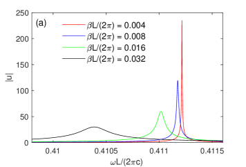
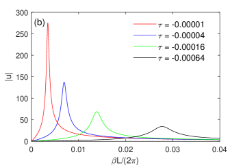
Figure 1: Example 1: Magnitude of the electric field at point $(0,0.2064L)$, (a) as a function of $\omega$, (b) as a function of $\beta$.

For each $\beta$, we also find the maximum of $|u|$ over all frequencies, and calculate the full width at half maximum (FWHM) $W_{\omega}$ for $|u|$ as a function of $\omega$. The results are listed in Table 2.

Table 2: Example 1: Maximum of $|u|$ as a function of $\omega$ for fixed $\beta$ and FWHM $W_{\omega}$.

$\beta L/(2\pi)$	$\max_{\omega}|u|$	$W_{\omega}$
0.004	238.8	0.71$\times$$10^{-5}$
0.008	119.4	2.82$\times$$10^{-5}$
0.016	59.76	1.13$\times$$10^{-4}$
0.032	29.96	4.45$\times$$10^{-4}$

The perturbation theory predicts that the maximum is reached when $\omega\approx\mbox{Re}(\omega_{*})$. This is true to high accuracy when $Q$ is large. It is also easy to see that $\max_{\omega}|u|\sim 1/\beta$, and this confirms the perturbation result that enhancement should be proportional to $1/\sqrt{Q}$. The values of $W_{\omega}$ in Table 2 indicate that $W_{\omega}\sim\beta^{2}$. From the perturbation theory of Sec. III, Eq. (28) in particular, we know that the leading term of $u$ is inversely proportional to $\omega-\mbox{Re}(\omega_{*})$. Thus, the maximum is obtained when $\omega\approx\mbox{Re}(\omega_{*})$, and half maximum is achieved when

$$\omega\approx\mbox{Re}(\omega_{*})\pm\sqrt{3}\,\mbox{Im}(\omega_{*}).$$ (34)

Therefore, $W_{\omega}\approx 2\sqrt{3}\,|\mbox{Im}(\omega_{*})|\sim\beta^{2}$.

We also study how the field depends on $\beta$ for a fixed frequency near the BIC frequency $\omega_{\circ}$. For this BIC, the real part of $\omega_{*}$ is less than $\omega_{\circ}$ as shown in Table 1. Therefore, we consider the dependence on $\beta$ for $\omega$ slightly less than $\omega_{\circ}$. The numerical results are shown in Fig. 1(b), where

$$\tau=(\omega-\omega_{\circ})L/(2\pi c).$$ (35)

We also calculate $\beta_{*}$ and $W_{\beta}$, where $\beta_{*}$ is the value of $\beta$ that gives the maximum of $|u|$, and $W_{\beta}$ is the FWHM for $|u|$ as a function of $\beta$. The results are listed in Table 3.

Table 3: Example 1: Maximum of $|u|$ attained at $\beta_{*}$ for fixed $\omega$, and FWHM $W_{\beta}$.

$(\omega-\omega_{\circ})L/(2\pi c)$	$\beta_{*}L/(2\pi)$	$\max_{\beta}|u|$	$W_{\beta}$
-0.00001	0.00344390	275.2	0.92$\times$$10^{-3}$
-0.00004	0.00690362	137.6	1.83$\times$$10^{-3}$
-0.00016	0.01381251	68.80	3.67$\times$$10^{-3}$
-0.00064	0.02766718	34.24	7.34$\times$$10^{-3}$

Since the leading term of $u$ is proportional to $1/[\omega-\omega_{*}(\beta)]$, $\beta_{*}$ should satisfy $\omega=\mbox{Re}[\omega_{*}(\beta_{*})]$ approximately. As $\mbox{Re}[\omega_{*}(\beta)]-\omega_{\circ}$ depends on $\beta$ quadratically, we easily obtain $\beta_{*}\sim|\omega-\omega_{\circ}|^{1/2}$. The maximum of $|u|$ is proportional to $\sqrt{Q}$ for that $\beta_{*}$, and thus it is proportional to $|\omega-\omega_{\circ}|^{-1/2}$. The two $\beta$ values at half maximum can be approximately calculated from the following equation

$$|\omega-\omega_{*}(\beta)|=2|\mbox{Im}[\omega_{*}(\beta_{*})]|$$ (36)

Using the leading order approximation for $\omega_{*}(\beta)-\omega_{\circ}$, it is easy to show that both solutions of Eq. (36), as well as their difference, scale as $|\omega-\omega_{\circ}|^{1/2}$. Therefore, $W_{\beta}\sim|\omega-\omega_{\circ}|^{1/2}$. All these asymptotic relations are confirmed by the numerical results listed in Table 3.

The second example is a symmetric standing wave on a periodic array of cylinders with dielectric constant $\epsilon_{s}=10$ and radius $r_{s}=0.36665158L$. The frequency of this BIC is $\omega_{\circ}=0.491142367(2\pi c/L)$. It is not a symmetry-protected BIC, since its field pattern is symmetric in $y$ (i.e. $u$ is even in $y$). It turns out that the BIC is also even in $x$. In Table 4,

Table 4: Example 2: Resonant modes near the BIC.

$\beta L/(2\pi)$	$(\omega_{*}-\omega_{\circ})L/(2\pi c)$	$Q$
0.01	0.000093965 - 0.000000025i	9.77$\times$$10^{6}$
$0.01\sqrt{2}$	0.000187712 - 0.000000093i	2.63$\times$$10^{6}$
0.02	0.000374556 - 0.000000358i	6.87$\times$$10^{5}$
$0.02\sqrt{2}$	0.000745686 - 0.000001393i	1.77$\times$$10^{5}$

we list the complex frequencies and $Q$-factors for a few resonant modes near the BIC. These results confirm that $\mbox{Re}(\omega_{*})-\omega_{\circ}\sim\beta^{2}$, $\mbox{Im}(\omega_{*})\sim\beta^{4}$, and $Q\sim 1/\beta^{4}$.

Next, we solve the diffraction problem with a plane incident wave, and monitor the solution at a particular point $(x,y)=(0,-0.3462L)$. In Fig. 2(a) and (b),

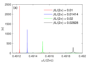
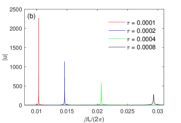
Figure 2: Example 2: Magnitude of the electric field at point $(0,-0.3462L)$, (a) as a function of $\omega$, (b) as a function of $\beta$.

we show $|u|$ at that point as a function of $\omega$ for fixed $\beta$ and as a function of $\beta$ for fixed $\omega$, respectively. For the case of fixed $\beta$, the maximum of $|u|$ and FWHM $W_{\omega}$ are listed in Table 5.

Table 5: Example 2: Maximum of $|u|$ as a function of $\omega$ for fixed $\beta$ and FWHM $W_{\omega}$.

$\beta L/(2\pi)$	$\max_{\omega}|u|$	$W_{\omega}$
0.01	2419	0.87$\times$$10^{-7}$
$0.01\sqrt{2}$	1210	3.23$\times$$10^{-7}$
0.02	605.5	1.24$\times$$10^{-6}$
$0.02\sqrt{2}$	303.2	4.82$\times$$10^{-6}$

These numerical results indicate that $\max|u|\sim 1/\beta^{2}$ and $W_{\omega}\sim\beta^{4}$, and they support our claims that field enhancement is proportional to $\sqrt{Q}$ and $W_{\omega}\approx 2\sqrt{3}\,|\mbox{Im}(\omega_{*})|$. From Table 4, we see that $\mbox{Re}(\omega_{*})$ is larger than $\omega_{\circ}$ for this BIC. Therefore, we show $|u|$ as functions of $\beta$ for $\omega$ slightly larger than $\omega_{\circ}$ in Fig. 2(b). For each fixed $\omega$, we list $\beta_{*}$, $\max_{\beta}|u|$ and FWHM $W_{\beta}$ in Table 6.

Table 6: Example 2: Maximum of $|u|$ attained at $\beta_{*}$ for fixed $\omega$, and FWHM $W_{\beta}$.

$(\omega-\omega_{\circ})L/(2\pi c)$	$\beta_{*}L/(2\pi)$	$\max_{\beta}|u|$	$W_{\beta}$
0.0001	0.01031652	2273	0.51$\times$$10^{-5}$
0.0002	0.01459880	1136	1.34$\times$$10^{-5}$
0.0004	0.02067137	566.9	3.66$\times$$10^{-5}$
0.0008	0.02930596	282.5	1.03$\times$$10^{-4}$

Since the maximum of $|u|$ is approximately attained when $\omega=\mbox{Re}(\omega_{*})$, we have $\beta_{*}\sim|\omega-\omega_{\circ}|^{1/2}$. This also implies that $\max_{\beta}|u|\sim\sqrt{Q}\sim 1/|\omega-\omega_{\circ}|$. To estimate $W_{\beta}$, we assume the equation $|\omega-\omega_{*}(\beta)|=2|\mbox{Im}[\omega_{*}(\beta_{*})]|$ has two solutions near $\beta_{*}$. The Taylor expansion at $\beta_{*}$ gives

$$\omega-\omega_{*}(\beta)=-\mbox{Im}[\omega_{*}(\beta_{*})]-\omega_{*}^{\prime}(\beta_{*})(\beta-\beta_{*})+...$$

where $\omega_{*}^{\prime}$ is the derivative of $\omega_{*}$ with respect to $\beta$. Therefore, the two terms in the right hand side above must have the same order. Since $\mbox{Im}[\omega_{*}(\beta_{*})]=O(\beta_{*}^{3})$ and $\omega_{*}^{\prime}(\beta_{*})=O(\beta_{*})$, we conclude that $\beta-\beta_{*}=O(\beta_{*}^{3})$. This leads to $W_{\beta}=O(\beta_{*}^{3})$ or $W_{\beta}\sim|\omega-\omega_{\circ}|^{3/2}$. The numerical results of Table 6 are consistent with these asymptotic relations. In particular, the last column of Table 6 confirm that when $|\omega-\omega_{\circ}|$ is increased by a factor of $2$, $W_{\beta}$ is increased by a factor of $2^{1.5}\approx 2.83$.

The third example is a propagating BIC on a periodic array of cylinders with $\epsilon_{s}=11.56$ and $r_{s}=0.35L$. The frequency and Bloch wavenumber of the BIC are $\omega_{\circ}=0.670236140(2\pi c/L)$ and $\beta_{\circ}=0.2483(2\pi/L)$, respectively. In Table 7,

Table 7: Example 3: Resonant modes near the BIC.

$(\beta-\beta_{\circ})L/(2\pi)$	$(\omega_{*}-\omega_{\circ})L/(2\pi c)$	$Q$-factor
0.004	0.00025157 - 0.00000127i	2.63$\times$$10^{5}$
0.008	0.00049981 - 0.00000518i	6.47$\times$$10^{4}$
0.016	0.00098439 - 0.00002120i	1.58$\times$$10^{4}$
0.032	0.00188950 - 0.00008790i	3.82$\times$$10^{3}$

we show the complex frequencies and $Q$-factors of a few resonant modes for $\beta$ near $\beta_{\circ}$. For this BIC, it is clear that $\mbox{Re}(\omega_{*})-\omega_{\circ}\sim\beta-\beta_{\circ}$, $\mbox{Im}(\omega_{*})\sim(\beta-\beta_{\circ})^{2}$, and $Q\sim 1/(\beta-\beta_{\circ})^{2}$.

For the diffraction problem with an incident wave of unit amplitude, we monitor the solution at point $(x,y)=(0.1526L,-0.2579L)$. In Fig. 3(a) and (b),

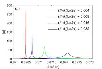
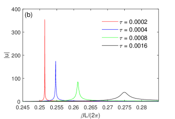
Figure 3: Example 3: Magnitude of the electric field at point $(0.1526L,-0.2579L)$, (a) as a function of $\omega$, (b) as a function of $\beta$.

we show $|u|$ at that point as functions of $\omega$ or $\beta$, respectively. For a few fixed values of $\beta-\beta_{\circ}$, the maximum of $|u|$ and FWHM $W_{\omega}$ are listed in Table 8.

Table 8: Example 3: Maximum of $|u|$ as a function of $\omega$ for fixed $\beta$ and FWHM $W_{\omega}$.

$(\beta-\beta_{\circ})L/(2\pi)$	$\max_{\omega}|u|$	$W_{\omega}$
0.004	280.6	4.41$\times$$10^{-6}$
0.008	138.7	1.80$\times$$10^{-5}$
0.016	68.10	7.40$\times$$10^{-5}$
0.032	32.87	3.05$\times$$10^{-4}$

These numerical results indicate that $\max_{\omega}|u|\sim 1/|\beta-\beta_{\circ}|$ and $W_{\omega}\sim|\beta-\beta_{\circ}|^{2}$, and they are consistent with the results on field enhancement and $W_{\omega}\approx 2\sqrt{3}\,\mbox{Im}(\omega_{*})\sim(\beta-\beta_{\circ})^{2}$. For a few fixed frequencies near $\omega_{\circ}$, we list $\max_{\beta}|u|$, $\beta_{*}$ and $W_{\beta}$ in Table 9.

Table 9: Example 3: Maximum of $|u|$ attained at $\beta_{*}$ for fixed $\omega$, and FWHM $W_{\beta}$.

$(\omega-\omega_{\circ})L/(2\pi c)$	$\beta_{*}L/(2\pi)$	$\max_{\beta}|u|$	$W_{\beta}$
0.0002	0.25147581	354.6	4.41$\times$$10^{-5}$
0.0004	0.25468389	174.5	1.84$\times$$10^{-4}$
0.0008	0.26121366	84.93	7.87$\times$$10^{-4}$
0.0016	0.27488676	39.93	3.75$\times$$10^{-3}$

The maximum of $|u|$ is attained at $\beta_{*}$ which satisfies $\omega=\mbox{Re}[\omega_{*}(\beta_{*})]$ approximately. Therefore, $\beta_{*}-\beta_{\circ}\sim\omega-\omega_{\circ}$. In addition, $\max_{\beta}|u|$ should be proportional to $\sqrt{Q}$ for the corresponding $\beta_{*}$. Therefore, $\max_{\beta}|u|\sim 1/|\beta_{*}-\beta_{\circ}|\sim 1/|\omega-\omega_{\circ}|$. To determine $W_{\omega}$, we first estimate the $\beta$ that gives half maximum. As before, we know that $\mbox{Im}[\omega_{*}(\beta_{*})]$ and $\omega_{*}^{\prime}(\beta_{*})(\beta-\beta_{*})$ should be on the same order, but $\omega_{*}^{\prime}(\beta_{*})]$ is a nonzero constant, thus $\beta-\beta_{\circ}\sim(\beta_{*}-\beta_{\circ})^{2}\sim(\omega-\omega_{\circ})^{2}$. Therefore, $W_{\beta}\sim(\omega-\omega_{\circ})^{2}$.

The fourth example is an antisymmetric standing wave on a periodic array with $\epsilon_{s}=8.2$ and $r_{s}=0.432266L$. The frequency of this BIC is $\omega_{\circ}=0.770094460005(2\pi c/L)$. In Table 10,

Table 10: Example 4: Resonant modes near the BIC.

$\beta L/(2\pi)$	$(\omega_{*}-\omega_{\circ})L/(2\pi c)$	$Q$-factor
0.005	-0.000036385554 - 0.000000000024i	1.63$\times$$10^{10}$
0.01	-0.000145089692 - 0.000000001751i	2.20$\times$$10^{8}$
0.02	-0.000573518292 - 0.000000102698i	3.75$\times$$10^{6}$
0.04	-0.002204078427 - 0.000004284774i	8.96$\times$$10^{4}$

we list the complex frequencies and $Q$-factors of a few resonant modes with $\beta$ close to $\beta_{\circ}=0$. It is quite clear that $\mbox{Re}(\omega_{*})-\omega_{\circ}\sim\beta^{2}$, $\mbox{Im}(\omega_{*})\sim\beta^{6}$, and $Q\sim 1/\beta^{6}$.

For the diffraction problem, we monitor the solution at $(x,y)=(0.1237L,0)$. The numerical results are shown in Fig. 4

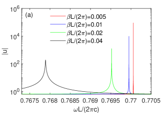
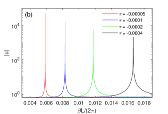
Figure 4: Example 4: Magnitude of the electric field at point $(0.1237L,0)$, (a) as a function of $\omega$, (b) as a function of $\beta$.

for fixed $\beta$ near $\beta_{\circ}=0$ and fixed $\omega$ near $\omega_{\circ}$. The maximum of $|u|$ for fixed $\beta$ are listed in Table 11.

Table 11: Example 4: Maximum of $|u|$ as a function of $\omega$ for fixed $\beta$ and FWHM $W_{\omega}$.

$\beta L/(2\pi)$	$\max_{\omega}|u|$	$W_{\omega}$
0.005	9.03$\times$$10^{4}$	8.2$\times$$10^{-11}$
0.01	9.67$\times$$10^{3}$	6.1$\times$$10^{-9}$
0.02	1.24$\times$$10^{3}$	3.6$\times$$10^{-7}$
0.04	1.89$\times$$10^{2}$	1.5$\times$$10^{-5}$

Since $\mbox{Im}(\beta_{*})\sim\beta^{6}$, we have $Q\sim 1/\beta^{6}$, $\max_{\omega}|u|\sim 1/\sqrt{Q}\sim 1/\beta^{3}$, and $W_{\omega}\approx 2\sqrt{3}\mbox{Im}(\omega_{*})\sim\beta^{6}$. In Table 12,

Table 12: Example 4: Maximum of $|u|$ attained at $\beta_{*}$ for fixed $\omega$, and FWHM $W_{\beta}$.

$(\omega-\omega_{\circ})L/(2\pi c)$	$\beta_{*}L/(2\pi)$	$\max_{\beta}|u|$	$W_{\beta}$
-0.00005	0.005862404	5.26$\times$$10^{4}$	1.3$\times$$10^{-8}$
-0.0001	0.008296643	1.72$\times$$10^{4}$	8.1$\times$$10^{-8}$
-0.0002	0.011749913	5.92$\times$$10^{3}$	4.7$\times$$10^{-7}$
-0.0004	0.016663279	2.10$\times$$10^{3}$	2.6$\times$$10^{-6}$

we list the maximum of $|u|$ for fixed $\omega$ slightly smaller than $\omega_{\circ}$. From the result on the real part of $\omega_{*}$, it is easy to show that $\beta_{*}\sim|\omega-\omega_{\circ}|^{1/2}$. Meanwhile, $\max_{\beta}|u|$ should be proportional to $\beta_{*}^{-3}$ or $|\omega-\omega_{\circ}|^{-1.5}$. As before, the two $\beta$ that reach half the maximum satisfy $\omega_{*}^{\prime}(\beta_{*})(\beta-\beta_{*})\sim\mbox{Im}[\omega_{*}(\beta_{*})]\sim\beta_{*}^{6}$. Since $\omega_{*}^{\prime}(\beta_{*})\sim\beta_{*}$, then both $|\beta-\beta_{*}|$ and $W_{\beta}$ are $O(\beta_{*}^{5})$. Therefore, $W_{\beta}\sim|\omega-\omega_{\circ}|^{2.5}$. The numerical results in Tables 11 and 12 confirm all these asymptotic results.

V Conclusions

Field enhancement by high-$Q$ resonances is crucial for realizing many applications in photonics. Since a BIC on a periodic structure is surrounded by resonant modes with $Q$-factors approaching infinity, it is important to develop asymptotic formulas for field enhancement around BICs. In this paper, we derived a formula for resonant field enhancement on 2D periodic structures (with 1D periodicity) sandwiched between two homogeneous media, and performed accurate numerical calculations for field enhancement around some BICs exhibiting different asymptotic relations. Although our study is for 2D structures, we expect the results still hold for 3D biperiodic structures such as photonic crystal slabs. Instead of varying the Bloch wavenumber, high-$Q$ resonant modes can also be created by perturbing the structure. The theory on field enhancement developed in Sec. III is also applicable to these resonances.

In practice, a small material loss is always present in any dielectric material, and it sets a limit for both the $Q$-factor and the field enhancement yoon15 . The material loss also has nontrivial effects on some BICs without symmetry protection huyuan19 . Further studies are needed to estimate the $Q$-factors and field enhancement for realistic structures that are finite, nonperiodic and lossy, and with fabrication errors that destroy the relevant symmetries.

Appendix A

Let $u$ be a resonant mode satisfying Eqs. (3) and (5). Multiplying $\overline{u}$ to both sides of Eq. (3), integrating on $\Omega$ and using integration by parts, we have

$$\int_{\partial\Omega}\overline{u}\frac{\partial u}{\partial\nu}ds-\int_{\Omega}|\nabla u|^{2}d{\bm{r}}+k^{2}\int_{\Omega}\epsilon|u|^{2}d{\bm{r}}=0,$$ (37)

where $\partial\Omega$ is the boundary of $\Omega$, $\nu$ is the outward unit normal vector of $\Omega$. Due to the quasi-periodic condition in $y$, the line integrals at $y=\pm L/2$ cancel, thus

$$\int_{\partial\Omega}\overline{u}\frac{\partial u}{\partial\nu}ds=\int_{-L/2}^{L/2}\left[\overline{u}\frac{\partial u}{\partial x}\right]^{x=D}_{x=-D}dy,$$

where $[F(x,y)]^{x=D}_{x=-D}=F(D,y)-F(-D,y)$. Evaluating the right hand side above using Eq. (5), we obtain

$$\int_{\partial\Omega}\overline{u}\frac{\partial u}{\partial\nu}ds=L\sum_{m=-\infty}^{\infty}i\alpha_{m}(|c_{m}^{+}|^{2}+|c_{m}^{-}|^{2}).$$ (38)

Taking the imaginary parts of Eqs. (37) and (38), we have

$$L\sum_{m}(|c_{m}^{+}|^{2}+|c_{m}^{-}|^{2})\mbox{Re}(\alpha_{m})+\mbox{Im}(k^{2})\int_{\Omega}\epsilon|u|^{2}d{\bm{r}}=0.$$

Let $\Omega_{e}^{+}$ be the domain given by $x>D$ and $|y|<L/2$, and $u_{e}$ be the sum of all terms with $m\neq 0$ in Eq. (5), then $u_{e}$ satisfies

$$(\partial_{x}^{2}+\partial_{y}^{2}+k^{2})u_{e}=0.$$

Multiplying the above by $\overline{u}_{e}$ and integrating on $\Omega_{e}^{+}$, we get

$$L\sum_{m\neq 0}|c_{m}^{+}|^{2}\mbox{Re}(\alpha_{m})=\mbox{Im}(k^{2})\int_{\Omega_{e}^{+}}|u_{e}|^{2}d{\bm{r}}.$$

A similar result holds for $\Omega_{e}^{-}$ given by $x<-D$ and $|y|<L/2$, then for $\Omega_{e}=\Omega_{e}^{+}\cup\Omega_{e}^{-}$, we have

$$L\sum_{m\neq 0}(|c_{m}^{+}|^{2}+|c_{m}^{-}|^{2})\mbox{Re}(\alpha_{m})=\mbox{Im}(k^{2})\int_{\Omega_{e}}|u_{e}|^{2}d{\bm{r}}.$$

Combining the above equations, we obtain

$$-\mbox{Im}(k^{2})\left(\int_{\Omega}\epsilon|u|^{2}d{\bm{r}}+\int_{\Omega_{e}^{+}}|u_{e}|^{2}d{\bm{r}}\right)$$

$$=L(|c_{0}^{+}|^{2}+|c_{0}^{-}|^{2})\mbox{Re}(\alpha_{0}).$$

Noticing that $\mbox{Im}(k^{2})=2\mbox{Re}(k)\mbox{Im}(k)$ and $1/Q=-2\mbox{Im}(k)/\mbox{Re}(k)$, the above leads to Eq. (16).

Appendix B

Multiplying Eq. (31) by $v_{*}$, integrating on $\Omega$, we get

$$\int_{\partial\Omega}\left(v_{*}\frac{\partial u_{0}}{\partial\nu}-u_{0}\frac{\partial v_{*}}{\partial\nu}\right)ds=-2Ck_{*}\int_{\Omega}\epsilon u_{*}v_{*}d{\bm{r}}.$$ (39)

In the above, we used Green’s second identity and noticed that $v_{*}$ satisfies the same Helmholtz equation as $u_{*}$. For the left hand side above, the line integrals at $y=\pm L/2$ cancel out, thus

$$\int_{\partial\Omega}v_{*}\frac{\partial u_{0}}{\partial\nu}ds=\int_{-L/2}^{L/2}\left[v_{*}\frac{\partial u_{0}}{\partial x}\right]^{x=D}_{x=-D}dy,$$

$$\int_{\partial\Omega}u_{0}\frac{\partial v_{*}}{\partial\nu}ds=\int_{-L/2}^{L/2}\left[u_{0}\frac{\partial v_{*}}{\partial x}\right]^{x=D}_{x=-D}dy.$$

For $\partial_{x}u_{0}$, we use the boundary condition (32). For $v_{*}$ and $\partial_{x}v_{*}$, we use the expansion (20). It is easy to verify that

$$\int_{-L/2}^{L/2}\left[v_{*}(B_{*}u_{0})-u_{0}\frac{\partial v_{*}}{\partial x}\right]_{x=D}dy=0.$$

Thus,

$$\int_{-L/2}^{L/2}\left[v_{*}\frac{\partial u_{0}}{\partial x}-u_{0}\frac{\partial v_{*}}{\partial x}\right]_{x=D}dy$$

$$=\int_{-L/2}^{L/2}\left[Cv_{*}(B_{1}u_{*})-2i\alpha_{0}^{*}a_{0}^{+}e^{i\beta y}v_{*}\right]_{x=D}dy$$

$$=iLk_{*}C\sum_{m}c_{m}^{+}d_{m}^{+}/\alpha_{m}^{*}-2iL\alpha_{0}^{*}a_{0}^{+}d_{0}^{+}.$$

A similar result holds for the line integral at $x=-D$. Therefore,

$$\int_{\partial\Omega}\left(v_{*}\frac{\partial u_{0}}{\partial\nu}-u_{0}\frac{\partial v_{*}}{\partial\nu}\right)ds+2iL\alpha_{0}^{*}(a_{0}^{+}d_{0}^{+}+a_{0}^{-}d_{0}^{-})$$ (40)

$$=iLk_{*}C\sum_{m=-\infty}^{\infty}\frac{c_{m}^{+}d_{m}^{+}+c_{m}^{-}d_{m}^{-}}{\alpha_{m}^{*}}.$$ (41)

Inserting Eq. (39) to Eq. (41), we obtain Eq. (33).

References

- (1) C. W. Hsu, B. Zhen, A. D. Stone, J. D. Joannopoulos, and M. Soljačić, “Bound states in the continuum,” Nat. Rev. Mater. 1, 16048 (2016).
- (2) K. Koshelev, G. Favraud, A. Bogdanov, Y. Kivshar, and A. Fratalocchi, “Nonradiating photonics with resonant dielectric nanostructures,” Nanophotonics 8, 725–745 (2019).
- (3) J. von Neumann and E. Wigner, “Über merkwürdige diskrete eigenwerte,” Z. Physik 50, 291-293 (1929).
- (4) A.-S. Bonnet-Bendhia and F. Starling, “Guided waves by electromagnetic gratings and nonuniqueness examples for the diffraction problem,” Math. Methods Appl. Sci. 17, 305-338 (1994).
- (5) P. Paddon and J. F. Young, “Two-dimensional vector-coupled-mode theory for textured planar waveguides,” Phys. Rev. B 61, 2090-2101 (2000).
- (6) S. G. Tikhodeev, A. L. Yablonskii, E. A Muljarov, N. A. Gippius, and T. Ishihara, “Quasi-guided modes and optical properties of photonic crystal slabs,” Phys. Rev. B 66, 045102 (2002).
- (7) S. P. Shipman and S. Venakides, “Resonance and bound states in photonic crystal slabs,” SIAM J. Appl. Math. 64, 322-342 (2003).
- (8) R. Porter and D. Evans, “Embedded Rayleigh-Bloch surface waves along periodic rectangular arrays,” Wave Motion 43, 29-50 (2005).
- (9) S. Shipman and D. Volkov, “Guided modes in periodic slabs: existence and nonexistence,” SIAM J. Appl. Math. 67, 687–713 (2007).
- (10) D. C. Marinica, A. G. Borisov, and S. V. Shabanov, “Bound states in the continuum in photonics,” Phys. Rev. Lett. 100, 183902 (2008).
- (11) J. Lee, B. Zhen, S. L. Chua, W. Qiu, J. D. Joannopoulos, M. Soljačić, and O. Shapira, “Observation and differentiation of unique high-Q optical resonances near zero wave vector in macroscopic photonic crystal slabs,” Phys. Rev. Lett. 109, 067401 (2012).
- (12) C. W. Hsu, B. Zhen, J. Lee, S.-L. Chua, S. G. Johnson, J. D. Joannopoulos, and M. Soljačić, “Observation of trapped light within the radiation continuum,” Nature 499, 188–191 (2013).
- (13) E. N. Bulgakov and A. F. Sadreev, “Bloch bound states in the radiation continuum in a periodic array of dielectric rods,” Phys. Rev. A 90, 053801 (2014).
- (14) Y. Yang, C. Peng, Y. Liang, Z. Li, and S. Noda, “Analytical perspective for bound states in the continuum in photonic crystal slabs,” Phys. Rev. Lett. 113, 037401 (2014).
- (15) B. Zhen, C. W. Hsu, L. Lu, A. D. Stone, and M. Soljačič, “Topological nature of optical bound states in the continuum,” Phys. Rev. Lett. 113, 257401 (2014).
- (16) Z. Hu and Y. Y. Lu, “Standing waves on two-dimensional periodic dielectric waveguides,” Journal of Optics 17, 065601 (2015).
- (17) X. Gao, C. W. Hsu, B. Zhen, X. Lin, J. D. Joannopoulos, M. Soljačić, and H. Chen, “Formation mechanism of guided resonances and bound states in the continuum in photonic crystal slabs,” Sci. Rep. 6, 31908 (2016).
- (18) R. Gansch, S. Kalchmair, P. Genevet, T. Zederbauer, H. Detz, A. M. Andrews, W. Schrenk, F. Capasso, M. Lončar, and G. Strasser, “Measurement of bound states in the continuum by a detector embedded in a photonic crystal,” Light: Science & Applications 5, e16147 (2016).
- (19) L. Li and H. Yin, “Bound states in the continuum in double layer structures,” Sci. Rep. 6, 26988 (2016).
- (20) L. Ni, Z. Wang, C. Peng, and Z. Li, “Tunable optical bound states in the continuum beyond in-plane symmetry protection,” Phys. Rev. B 94, 245148 (2016).
- (21) L. Yuan and Y. Y. Lu, “Propagating Bloch modes above the lightline on a periodic array of cylinders,” J. Phys. B: Atomic, Mol. and Opt. Phys. 50, 05LT01 (2017).
- (22) E. N. Bulgakov and D. N. Maksimov, “Bound states in the continuum and polarization singularities in periodic arrays of dielectric rods,” Phys. Rev. A 96, 063833 (2017).
- (23) Z. Hu and Y. Y. Lu, “Resonances and bound states in the continuum on periodic arrays of slightly noncircular cylinders,” J. Phys. B: At. Mol. Opt. Phys. 51, 035402 (2018).
- (24) H. M. Doeleman, F. Monticone, W. den Hollander, A. Alù, and A. F. Koenderink, “Experimental observation of a polarization vortex at an optical bound state in the continuum,” Nature Photonics 12, 397–401 (2018).
- (25) Y. Zhang, A. Chen, W. Liu, C. W. Hsu, B. Wang, F. Guan, X. Liu, L. Shi, L. Lu, and J. Zi, “Observation of polarization vortices in momentum space,” Phys. Rev. Lett. 120, 186103 (2018).
- (26) L. Yuan and Y. Y. Lu, “Bound states in the continuum on periodic structures: perturbation theory and robustness,” Opt. Lett. 42(21) 4490-4493 (2017).
- (27) K. Koshelev, S. Lepeshov, M. Liu, A. Bogdanov, and Y. Kibshar, “Asymmetric metasurfaces with high- resonances governed by bound states in the contonuum,” Phys. Rev. Lett. 121, 193903 (2018).
- (28) L. Yuan and Y. Y. Lu, “Perturbation theories for symmetry-protected bound states in the continuum on two-dimensional periodic structures,” arXiv preprint arXiv:1911.03612 (2019).
- (29) L. Yuan and Y. Y. Lu, “Strong resonances on periodic arrays of cylinders and optical bistability with weak incident waves,” Phys. Rev. A 95, 023834 (2017).
- (30) L. Yuan and Y. Y. Lu, “Bound states in the continuum on periodic structures surrounded by strong resonances,” Phys. Rev. A 97, 043828 (2018).
- (31) J. Jin, X. Yin, L. Ni, M. Soljacic, B. Zhen, and C. Peng, “Topologically enable unltra-high- guided resonances robust to out-of-plane scattering,” Nature 574, 501-504 (2019).
- (32) A. Kodigala, T. Lepetit, Q. Gu, B. Bahari, Y. Fainman, and B. Kanté, “Lasing action from photonic bound states in continuum,” Nature 541, 196-199 (2017).
- (33) S. Romano, A. Lamberti, M. Masullo, E. Penzo, S. Cabrini, I. Rendina, and V. Mocella, “Optical biosensors based on photonic crystals supporting bound states in the continuum,” Materials 11, 526 (2018).
- (34) F. Yesilkoy, E. R. Arvelo, Y. Jahani, M. Liu, A. Tittl, V. Cevher, Y. Kivshar, and H. Altug, “Ultrasensitive hyperspectral imaging and biodetection enabled by dielectric metasurfaces,” Nature Photonics 13, 390-396 (2019).
- (35) L. Yuan and Y. Y. Lu, “Diffraction of plane waves by a periodic array of nonlinear circular cylinders,” Phys. Rev. A 94, 013852 (2016).
- (36) L. Yuan and Y. Y. Lu, “Excitation of bound states in the continuum via second harmonic generations,” arXiv preprint arXiv:1908.00137 (2019).
- (37) S. P. Shipman and S. Venakides, “Resonant transmission near nonrobust periodic slab modes,” Phys. Rev. E 71, 026611 (2005).
- (38) V. Mocella and S. Romano, “Giant field enhancement in photonic lattices,” Phys. Rev. B 92, 155117 (2015).
- (39) J. W. Yoon, S. H. Song, and R. Magnusson, “Critical field enhancement of asymptotic optical bound states in the continuum,” Sci. Rep. 5, 18301 (2015).
- (40) S. Fan and J. D. Joannopoulos, “Analysis of guided resonances in photonic crystal slabs,” Phys. Rev. B 65, 235112 (2002).
- (41) A. Abdrabou and Y. Y. Lu, “Indirect link between resonant and guided modes on uniform and periodic slabs,” Phys. Rev. A 99, 063818 (2019).
- (42) G. Bao, D. C. Dobson, and J. A. Cox, “Mathematical studies in rigorous grating theory,” J. Opt. Soc. Am. A 12(5), 1029-1042 (1995).
- (43) Z. Hu, L. Yuan, and Y. Y. Lu, “Bound states with complex frequencies near the continuum on lossy periodic structures,” arXiv preprint arXiv:1910.02229 (2019).