A greedy algorithm for computing eigenvalues
of a symmetric matrix

Abstract

We present a greedy algorithm for computing selected eigenpairs of a large sparse matrix $H$ that can exploit localization features of the eigenvector. When the eigenvector to be computed is localized, meaning only a small number of its components have large magnitudes, the proposed algorithm identifies the location of these components in a greedy manner, and obtains approximations to the desired eigenpairs of $H$ by computing eigenpairs of a submatrix extracted from the corresponding rows and columns of $H$. Even when the eigenvector is not completely localized, the approximate eigenvectors obtained by the greedy algorithm can be used as good starting guesses to accelerate the convergence of an iterative eigensolver applied to $H$. We discuss a few possibilities for selecting important rows and columns of $H$ and techniques for constructing good initial guesses for an iterative eigensolver using the approximate eigenvectors returned from the greedy algorithm. We demonstrate the effectiveness of this approach with examples from nuclear quantum many-body calculations, many-body localization studies of quantum spin chains and road network analysis.

Keywords

eigenvector localization, greedy algorithm, large-scale eigenvalue problem, perturbation analysis

1 Introduction

Large-scale eigenvalue problems arise from many scientific applications. In some of these applications, we are interested in a few eigenvalues of a large sparse symmetric matrix. These eigenvalues may be the smallest algebraically or largest in magnitude, etc. The dimension of these problems can be extremely large. For example, in quantum many-body calculations, the dimension of the matrix depends on the number of particles and approximation model parameters. It can grow rapidly with respect to the size of the problem and accuracy requirement. For internet, social, road or traffic network analysis, the dimension of the adjacency matrix of the network, which describes the interconnection of different nodes of the network, depends on the number of nodes of the network, which can increase rapidly on a daily basis. However, these matrices are often sparse. Because only a small fraction of the matrix elements are nonzero, and since only a small number of eigenpairs are desired, iterative methods are often used to solve this type of problem. The dominant cost of these methods is in performing a sparse matrix vector multiplication at each step of the iterative solver. For large problems, performing this calculation efficiently on a high performance computer is a challenging task. Not only do we need to choose an appropriate data structure to represent the sparse matrix, we also need to develop efficient schemes to distribute the matrix and vectors on multiple nodes or processors to overcome the single node memory limitation and enable the computation to be performed in parallel.

It is well known that, for some problems, the eigenvector to be computed has localization properties, i.e., many elements of the desired eigenvector are negligibly small [11, 17]. For example, in quantum many-body problems, localization means that the many-body operator of interest can be represented by a few many-body basis functions in a small configuration space. This feature of the problem implies that the rows and columns associated with the large elements of the eigenvectors are more “important” than others. We can then effectively work with a much smaller matrix by excluding rows and columns associated with small elements in the eigenvector. In network analysis problems, the localization of the principal eigenvector, i.e., the eigenvector associated with the largest (in magnitude) eigenvalue often reveals a densely connected subgraph or cluster in the network [19].

However, in general, we do not know which elements of the eigenvector are small (in magnitude) in advance. In some cases, there are efficient numerical procedures that can be used to identify these elements, e.g., the latest work by Arnold et al. [2, 1]. But these techniques may require solving another large problem such as a large linear system of equations. There are sometimes physical intuitions we may use to infer which rows/columns are more important than others. For example, in a configuration interaction approach for quantum many-body problems, the matrix to be partially diagonalized is the representation of the Hamiltonian in a many-body basis that consists of antisymmetric products (Slater determinants) of a set of single-particle basis functions, e.g., eigenfunctions of a quantum harmonic oscillator. Many-body basis functions defined by single-particle functions associated with lower single-particle energies tend to be more “important” than others, although this is not always true. In a network analysis problem, nodes with large degrees or other attributes such as centrality tend to form the center of a densely connected subgraph, and thus are deemed more “important” than others.

In this paper, we describe a greedy algorithm to incrementally probe large components of a localized eigenvector to be computed. The matrix rows and columns corresponding to these components are extracted to construct a much smaller matrix. The eigenvector of this small matrix is then used to obtain an approximate eigenvector of the original matrix to be partially diagonalized. If the approximate eigenpair is not sufficiently accurate (the metric for measuring accuracy will be described below), we select some additional rows and columns of the original matrix and solve a slightly larger problem using the solution of the previous problem as the starting guess. This procedure can be repeated recursively until the computed eigenpair is sufficiently accurate.

For problems that are not strictly localized, i.e., many eigenvector components are small but not zero, this approach does not completely eliminate the need to use an iterative method to compute the desired eigenpair of the original matrix. However, the number of iterations required to reach convergence can be significantly reduced if a good starting guess can be constructed from the greedy scheme. If the submatrices selected by the greedy algorithm are relatively small, the cost of computing the desire eigenpairs of these smaller matrices is relatively low. Consequently, the overall cost of the computation can be reduced.

We should note that the greedy algorithm proposed in this paper is different from the hierarchical algorithm presented by Shao et al. [23]. Instead of using a predefined set of hierarchical configuration spaces to construct a sequence of submatrices from which approximate eigenpairs are computed, the greedy algorithm constructs these submatrices dynamically using the previous approximate eigenvector to guide such a construction.

The greedy strategy used to construct a sequence of submatrices from which approximate eigenpairs are computed is similar to the so-called selected configuration interaction approach used in quantum chemistry [30, 15, 32, 22, 8, 5, 24, 25, 6] and the importance truncation scheme used in nuclear physics [21]. But we would like to emphasize that the techniques discussed here are more general. They are not restricted to problems arising from quantum chemistry or physics. Moreover, we describe greedy strategies in terms of matrices and vectors instead of many-body configurations and Hamiltonians. As a result, these strategies can potentially be applied to other applications such as sparse principal component analysis [33].

This paper is organized as follows. In section 2, we discuss the implication of eigenvector localization on the development of an efficient iterative method for computing such an eigenvector, and outline the general strategy for developing such an algorithm. In section 3, we discuss several greedy strategies for selecting rows and columns of the original matrix to construct a submatrix from which approximate eigenpairs are computed and used as a starting guess for computing the eigenpairs of the original problem. Techniques for improving the starting guess are discussed in section 4. In section 5, we present some numerical examples to demonstrate the efficiency of the greedy algorithm. Additional improvement of the algorithm is discussed in section 6.

2 Eigenvector localization and a hierarchical method for computing localized eigenvectors

Let $H\in\mathbb{R}^{n\times n}$ be the symmetric matrix to be partially diagonalized. To simplify our discussion, let us focus on computing the algebraically smallest eigenvalue $\lambda$ of $H$ and its corresponding eigenvector $x$. If the desired eigenvector $x$ is localized, i.e., only a subset of its elements are nonzero, we can reorder the elements of the eigenvector to have all nonzero elements appear in the leading $n_{1}$ rows, i.e.,

$$Px=\begin{bmatrix}x_{1}\\ 0\end{bmatrix},$$

where $x_{1}\in\mathbb{R}^{n_{1}}$ and $P$ the permutation matrix associated with such a reordering. Consequently, we can reorder the rows and columns of the matrix $H$ so that

$$(PHP^{T})(Px)=\begin{bmatrix}H_{1}&B\\ B^{T}&C\end{bmatrix}\begin{bmatrix}x_{1}\\ 0\end{bmatrix}=\lambda\begin{bmatrix}x_{1}\\ 0\end{bmatrix}$$ (1)

holds. To obtain $x_{1}$, we only need to solve the eigenvalue problem

$$H_{1}x_{1}=\lambda x_{1}.$$ (2)

Even when $x$ is not strictly localized, i.e., the magnitude of the elements in $x_{1}$ are significantly larger than the other elements that are small but not necessarily zero, the solution of (2) can be used to construct a good initial guess of $x$ that can be used to accelerate the convergence of an iterative method applied to compute the desired eigenpair of $H$.

However, since we do not know how large the elements of $x$ are in advance, we do not have the permutation $P$ that allows us to pick rows and columns of $H$ to form $H_{1}$.

The algorithm presented in this paper seeks to identify the permutation $P$ that allows us to construct $H_{1}$ incrementally so that successively more accurate approximations to the desired eigenpair can be obtained efficiently. The basic algorithm we use to achieve this goal can be described as follows.

1. We select a subset of the indices $1,2,...,n$ denoted by $\mathcal{S}$ that corresponds to “important” rows and columns of $H$. These rows and columns define a submatrix $H_{1}$ of $H$. We will comment further on possible approaches to selecting $\mathcal{S}$, and therefore $H_{1}$, in Section 3.3. For instance, in the configuration interaction method for solving quantum many-body eigenvalue problems, this subset may correspond to a set of many-body basis functions produced from some physically-motivated basis truncation scheme.

2. Assuming the size of $\mathcal{S}$ is small relative to $n$, we can easily compute the desired eigenpair $(\lambda_{1},x_{1})$ of $H_{1}$, i.e., $H_{1}x_{1}=\lambda_{1}x_{1}$.

3. We take $\lambda_{1}$ to be the approximation to the smallest eigenvalue of $H$. The approximation to the eigenvector of $H$ is constructed as $\hat{x}=P^{T}\begin{bmatrix}x_{1}^{T}&0\end{bmatrix}^{T}$. To assess the accuracy of the computed eigenpair $(\lambda_{1},\hat{x})$, we compute the full residual $r=H\hat{x}-\lambda_{1}\hat{x}$.

4. If the norm of $r$ is sufficiently small, we terminate the computation and return $(\lambda_{1},\hat{x})$ as the approximate solution. Otherwise, we select some additional rows and columns of $H$ to augment $H_{1}$ and repeat steps 2–4 again.

If the eigenvector to be computed is localized, this procedure should terminate before the dimension of $H_{1}$ becomes very large, assuming that we can identify the most important rows and columns of $H$ in some way.

We should note that we permute $H$ so that $H_{1}$ becomes the leading principal submatrix merely for convenience. Such a permutation makes our analysis more clear. But in a practical computational procedure, as long as we can identify and access rows and columns of $H$ that form the submatrix $H_{1}$, we do not need to explicitly move them to the leading rows and columns of $H$.

3 Greedy algorithms for detecting localization

Without loss of generality, we take $\mathcal{S}$ to be the leading $n_{1}$ rows and columns of $H$ so that we can partition $H$ as

$$H=\begin{bmatrix}H_{1}&B\\ B^{T}&C\end{bmatrix}.$$ (3)

We now discuss how to select additional “important” rows and columns outside of the subset $\mathcal{S}$ to obtain a more accurate approximation of the desired eigenvector of $H$.

3.1 Residual based approach

Suppose $(\lambda_{1},x_{1})$ is the computed eigenpair of the submatrix $H_{1}$ that serve as an approximation to the desired eigenpair $(\lambda,x)$. By padding $x_{1}$ with zeros to form

$$\hat{x}=\begin{bmatrix}x_{1}\\ 0\end{bmatrix},$$ (4)

we can assess the accuracy of the approximate eigenvector $\hat{x}$ in the full space by computing its residual

$$r=H\hat{x}-\lambda_{1}\hat{x}=\begin{bmatrix}0\\ B^{T}x_{1}\end{bmatrix}\equiv\begin{bmatrix}0\\ r^{\prime}\end{bmatrix}.$$ (5)

A first greedy scheme for improving the accuracy of $x_{1}$ is to select $k$ row and column indices in $\{1,2,...,n\}\setminus\mathcal{S}$ that correspond to components of $r^{\prime}=B^{T}x_{1}$ with the largest magnitude. These indices, along with $\mathcal{S}$, yield an augmented $H_{1}$ from which a more accurate approximation to $(\lambda,x)$ can be obtained.

3.2 Perturbation analysis based approach

It is possible that a component of $r^{\prime}$ is large in magnitude even though the magnitude of the corresponding component in the eigenvector $x$ is relatively small, or vice versa. Therefore, instead of selecting row and column indices that correspond to the components of the largest magnitude within $r^{\prime}$, it may be that a better selection can be made by estimating the magnitude of the components of $x$ whose corresponding indices are outside of $\mathcal{S}$, and then selecting the row and column indices that correspond to these estimated largest elements.

To do that, let us modify the $j$th component of the zero block of $\hat{x}$ in (4) and assume the vector

$$\tilde{x}=\begin{bmatrix}x_{1}\\ \gamma e_{j}\end{bmatrix}$$ (6)

is a better approximation to the eigenvector $x$ than $\hat{x}$ defined in (4), with the corresponding eigenvalue approximation $\tilde{\lambda}=\lambda_{1}+\delta$, where $\delta$ is the correction to the eigenvalue, and $e_{j}$ is the $j$th column of the $(n-n_{1})\times(n-n_{1})$ identity matrix.

Substituting (6) and $\tilde{\lambda}=\lambda_{1}+\delta$ into $Hx=\lambda x$ and examining the $(n_{1}+j)$th row of the equation yields

$$e_{j}^{T}B^{T}x_{1}+\gamma e_{j}^{T}Ce_{j}=(\lambda_{1}+\delta)\gamma.$$ (7)

If $(\lambda_{1},\hat{x})$ is a good approximation to $(\lambda,x)$, i.e., both $|\delta|$ and $|\gamma|$ are relatively small, we can drop the second order correction term $\delta\gamma$ and rearrange the equation to obtain

$$(\lambda_{1}-e_{j}^{T}Ce_{j})\gamma\approx e_{j}^{T}B^{T}x_{1}.$$ (8)

As a result, the $(n_{1}+j)$th component of $x$ can be estimated to be

$$\gamma\approx\frac{e_{j}^{T}B^{T}x_{1}}{\lambda_{1}-C_{j,j}},$$ (9)

where $C_{j,j}=e_{j}^{T}Ce_{j}$ is the $j$ diagonal element of the matrix $C$.

The magnitude of this quantity $\gamma$ in (9), the perturbation analysis estimate for the $(n_{1}+j)$th eigenvector component, is then taken to provide an estimate for the importance of the corresponding row and column of $H$ in a greedy selection approach. We should note that this approach is not new and has appeared in, for example,  [6] and  [8]. If we compare with the corresponding component $e_{j}^{T}r^{\prime}=e_{j}^{T}B^{T}x_{1}$ of the residual vector $r$, calculated above in (5) to provide an estimate of the importance of this row and column of $H$ in the residual based greedy selection approach, we see that the quantities used to estimate the importance of a row and column in the two approaches only differ by a scaling factor $|\lambda_{1}-C_{j,j}|^{-1}$.

In (6), we limit the perturbation to exactly one component in the zero block of $\hat{x}$ in (4). This is the approach taken in references [6, 30]. We will refer to this type of perturbation as componentwise perturbation.

It is conceivable that perturbing several components in this block may result in a better approximation of $x$. In the extreme case, all components of the zero block can be perturbed to yield a better approximation. In that case, we can express the perturbed approximation to the desired eigenvector as

$$\tilde{x}=\begin{bmatrix}x_{1}\\ z\end{bmatrix}.$$ (10)

Substituting (10) into $Hx=\lambda x$ and examine the second block of the equation yields

$$B^{T}x_{1}+Cz=(\lambda_{1}+\delta)z.$$ (11)

Again, if we drop the second order correction term $\delta z$ and rearrange the equation, we obtain

$$z\approx(\lambda_{1}I-C)^{-1}B^{T}x_{1}.$$ (12)

From (12) we can see that a full correction of the zero component of $\hat{x}$ requires solving a linear equation with the shifted matrix $\lambda_{1}I-C$ as the coefficient. This is likely to be prohibitively expensive because the dimension of $C$ is assumed to be much larger than the dimension of $H_{1}$. However, because all we need is the magnitudes of the components of $z$ relative to each other, which we will use to select the next set of rows and columns of $B$ and $C$ to be included in $H_{1}$, we do not necessarily need to solve the linear equation accurately. We will refer to this type of perturbation as full perturbation.

There are a number of options to obtain an approximate solution to (11). One possibility is to use an iterative solver such as the minimum residual (MINRES) algorithm [18], and perform a few iterations to obtain an approximation to $z$. We should note that eigenvalues of $C$ are larger than the smallest eigenvalue of $H$. However, the approximation to the smallest eigenvalue, $\lambda_{1}$, may not satisfy this condition, i.e., $C-\lambda_{1}I$ is not guaranteed to be positive definite. Therefore, it is better to use MINRES instead of the conjugate gradient algorithm to solve (11). Another possibility is to approximate the matrix $C$ by another matrix that is much easier to invert. For example, if $C$ is diagonally dominant, we can replace $C$ with a diagonal matrix $D$ that contains the diagonal of $C$. This approach will yield the same selection criterion as that provided by (9). When $C$ is not diagonal dominant, we may also include a few subdiagonal and superdiagonal bands to form a banded matrix approximation to $C$. Another possibility is to replace $C$ with a block diagonal matrix $G$ with relatively small diagonal blocks. This approach corresponds to perturbing a few rows of the zero block of $\hat{x}$ at a time. In this approach, it is important to block rows and columns of $C$ in such a way that $C=G+E$ for some matrix $E$ that is relatively small (in a matrix norm).

3.3 The initial choice of $H_{1}$

The success of the greedy algorithm outlined in section 2 and detailed in sections 3 and 4 depends, to a large degree, on the initial choice of rows and columns of $H$ we select to form the initial $H_{1}$. Such a choice is generally application dependent. For example, for molecular and nuclear configuration interaction calculations, rows and columns of $H$ that are associated with low excitation Slater determinants, i.e., Slater determinants that consist of single particle basis functions labeled with low quantum numbers, are often good choices. For network analysis problems, a good choice of rows and columns of $H$ are those associated with nodes in the network with the largest degrees and their neighbors. For some problems, it may be possible to start with a random selection of the rows and columns.

The number of rows and columns to be selected is also problem dependent. Choosing a larger number of rows and columns is likely to improve the overall convergence of the greedy algorithm and ensure the method to converge to the desired eigenpair. On the other hand, when too many rows and columns are chosen, the cost of computing the desired eigenpair of $H_{1}$ may be close to that of computing the desired eigenpair of $H$, which may defeat the purpose of developing the greedy algorithm.

4 Updating the Eigenvector Approximation

Once new row and column indices have been selected using the criteria discussed in the previous section, we update $H_{1}$ by including the additional rows and columns of $B$ and $C$ specified by the new row and column indices. We then compute the desired eigenvalue and the corresponding eigenvector of the updated $H_{1}$.

Since we already have the approximate eigenvector $x_{1}$ associated with the previous $H_{1}$, we hope to obtain the new approximation quickly by using an iterative method that can take advantage of a good starting guess of the desired eigenvector.

In this paper, we consider both the Lanczos method [12], which extracts approximate eigenpairs from the Krylov subspace

$$\mathcal{K}(H_{1},v_{0})=\mathrm{span}\left\{v_{0},H_{1}v_{0},H_{1}^{2}v_{0},\cdots,H_{1}^{m-1}v_{0}\right\},$$

where $v_{0}$ is the starting guess of the desired eigenvector, and the locally optimal block preconditioned conjugate gradient (LOBPCG) method [9]. In the LOBPCG method, the approximate eigenvector $x^{(j)}$ is updated successively according to the following updating formula

$$x^{(j+1)}=\alpha x^{(j)}+\beta Pr^{(j)}+\eta x^{(j-1)},$$

where $r^{(j)}=H_{1}x^{(j)}-\lambda^{(j)}x^{(j)}$ is the residual associated with the approximate eigenpair $(\lambda^{(j)},x^{(j)})$, $P$ is a properly chosen preconditioner, and the scalars $\alpha$, $\beta$, and $\eta$ are chosen to minimize the Rayleigh quotient $\langle x^{(j+1)},H_{1}x^{(j+1)}\rangle$, subject to the normalization constraint $\langle x^{(j+1)},x^{(j+1)}\rangle=1$. In addition to its ability to accelerate convergence by incorporating a preconditioner $P$ when one is available, the LOBPCG method can also take advantage of approximations to several eigenvectors simultaneously. However, in this paper, we will focus on computing the lowest eigenvalue of $H$ and its corresponding eigenvector.

There are a number of ways to choose the starting guess for both the Lanczos method and the LOBPCG method. The simplest approach is to construct the starting guess by padding $x_{1}$ with additional zeros. Another possibility is to pad $x_{1}$ with the largest components (in magnitude) of the approximate solution $z$ defined by (12), especially if (12) is used to select the new rows and columns of $B$ and $C$ to be included in $H_{1}$. This approach may work well if components of $x_{1}$ are already very close to the corresponding components in the exact eigenvector $x$. However, if that is not the case, we need to correct $x_{1}$ as well by defining $\tilde{x}$ as

$$\tilde{x}=\begin{bmatrix}x_{1}+z_{1}\\ z_{2}\end{bmatrix},\qquad x_{1}^{T}z_{1}=0.$$ (13)

Substituting $\tilde{x}$ and $\lambda=\lambda_{1}-\delta$ into $Hx=\lambda x$, enforcing the $x_{1}^{T}z_{1}=0$ constraint, and dropping the second order perturbation term yields

$$\begin{bmatrix}H_{1}&B&x_{1}\\ B^{T}&C-\lambda_{1}I&0\\ x_{1}^{T}&0&0\end{bmatrix}\begin{bmatrix}z_{1}\\ z_{2}\\ \delta\end{bmatrix}=\begin{bmatrix}0\\ -B^{T}x_{1}\\ 0\end{bmatrix}.$$ (14)

Eliminating $\delta$ from (14) and applying the projector

$$\begin{bmatrix}I-x_{1}x_{1}^{T}&0&0\\ 0&I&0\\ 0&0&1\end{bmatrix}$$

to both sides of the equation results in

$$\begin{bmatrix}\hat{H}_{1}&\hat{B}\\ \hat{B}^{T}&C-\lambda_{1}I\end{bmatrix}\begin{bmatrix}z_{1}\\ z_{2}\end{bmatrix}=\begin{bmatrix}0\\ -B^{T}x_{1}\end{bmatrix},$$ (15)

where $\hat{H}_{1}=(I-x_{1}x_{1}^{T})(H_{1}-\lambda_{1}I)(I-x_{1}x_{1}^{T})$ and $\hat{B}=(I-x_{1}x_{1}^{T})B$. Note that the above derivation of the correction equation (15) is similar to that used in the development of the Jacobi-Davidson algorithm [26].

We can solve (15) by using an iterative solver such as the MINRES algorithm. Instead of adding $z_{1}$ and $z_{2}$ directly to $\begin{bmatrix}x_{1}^{T}&0\end{bmatrix}^{T}$ as shown in (13), we can project $H$ into a two-dimensional subspace spanned by

$$Q=\left\{\begin{bmatrix}x_{1}\\ 0\end{bmatrix},\begin{bmatrix}z_{1}\\ z_{2}\end{bmatrix}\right\},$$

and solving a $2\times 2$ eigenvalue problem. If $g_{1}$ is the eigenvector associated with the smallest eigenvalue of the projected matrix, the starting guess of the desired eigenvector of $H$ can be chosen as

$$\tilde{x}=Qg_{1}.$$

We will refer to this approach of preparing the starting guess as the Newton correction.

5 Numerical examples

In this section, we demonstrate the effectiveness of the greedy algorithm for computing the lowest eigenvalue of $H$ for three different applications. The first one arises from nuclear structure calculations. The second is concerned with computing the localized eigenvector of a model many-body Hamiltonian that includes local interactions and a disordered potential term. The third is related to computing the principal eigenvector of an adjacency matrix associated with a network graph. Our computations are performed on a Microsoft Surface Laptop 2 with an Intel Core i7-8650 chip running at 1.9Ghz, and 16GB memory. Our code is written in MATLAB and the version of MATLAB we use is R2018a.

Before presenting the results of the numerical experiments, we first describe 2 reference calculations, the 3 different variants of the greedy algorithm to be compared, and the Newton correction approach below:

• original: reference calculation by directly solving the full problem and using a random vector as initial guess.

• hierarch: reference calculation by exploiting the hierarchical structure of the matrix $H$, i.e., first solving the small problem, next padding the obtained small eigenvector with zeros and using it as initial guess for the full problem.

• greedy-res: greedy algorithm which uses the residual based approach for selecting the row and column indices to augment $H$ with.

• greedy-pert: greedy algorithm which uses the componentwise perturbation analysis based approach (9) for selecting the row and column indices to augment $H$ with.

• greedy-pert-full: greedy algorithm which uses the full perturbation analysis based approach (12) for selecting the row and column indices to augment $H$ with.

• newton-corr: Newton correction approach (13) for updating the eigenvector and initial guess.

5.1 Nuclear Configuration Interaction

The matrix $H$ to be partially diagonalized in this example is the nuclear many-body Schrödinger Hamiltonian for the nucleus of a lithium atom, in particular, of the isotope $\isotope[6]{Li}$, for which the nucleus consists of 3 protons and 3 neutrons. The matrix approximation to the nuclear Schrödinger Hamiltonian operator is constructed on the so-called configuration interaction space, spanned by a set of many-body basis functions.

Each of these many-body basis functions is a Slater determinant of a set of eigenfunctions of a 3D harmonic oscillator. These single-particle eigenfunctions are indexed by a set of quantum numbers $\{n(a),l(a),j(a),m(a)\}$, for each nucleon $a$, and is associated with number $N(a)=2n(a)+l(a)$ of oscillator quanta [29]. In the nuclear physics applications, the selection of Slater determinants for the configuration space is often done by specifying a limit on the sum of the oscillator quanta $N_{\mathrm{tot}}=\sum_{a}[2n(a)+l(a)]$ (some additional constraints are imposed on the quantum numbers to ensure appropriate symmetry properties) [3]. This limit on the oscillator quanta is often expressed in terms of a cutoff parameter $N_{\max}$ indicating the limit on the number of quanta permitted above the minimal number $N_{0}$ possible (that is, consistent with the Pauli principle, or antisymmetry of Slater determinants) for that nucleus: then the many-body basis function is restricted to $N_{\mathrm{tot}}\leq N_{0}+N_{\max}$. This constraint defines a truncation relative to the full configuration space, defined by all possible Slater determinants that can be generated, from a given set of harmonic oscillator eigenfunctions. The larger the $N_{\max}$, the larger the dimension of the matrix approximation $H$ to the Hamiltonian, and the higher the cost to obtain the desired eigenpairs of $H$.

We consider only two-body potential interactions. The finite dimensional Hamiltonian constructed from a truncated configuration space is sparse. Figure 1(a) shows the nonzero matrix element pattern of $H$ for the $N_{\max}=6$ truncation level. The dimension of this matrix is 197,882. A lexicographical ordering of the many-body (Slater determinant) basis by its single particle quantum numbers presented in [27] is used. This ordering preserves the $N_{\max}$ model truncation hierarchy. Under such a ordering scheme, the leading $800\times 800$ principal submatrix of $H$ corresponds to the Hamiltonian truncated with $N_{\max}=2$.

As a reference, we use the LOBPCG algorithm to compute the lowest eigenvalue and its eigenvector of $H$ for $N_{\max}=6$. For simplicity, no preconditioner is used here. However, an effective preconditioner such as the block diagonal preconditioner presented in [23] can be used. We plot the magnitude of its components in Figure 1(b). As we can see, many of these components are small.

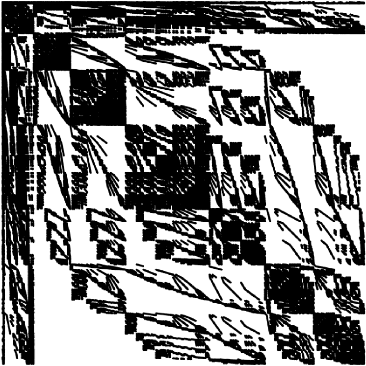
(a) The sparsity pattern of the $\isotope[6]{Li}$ Hamiltonian.

nci-eigvec [ width=0.95height=0.95xmin=0, xmax=197900, scaled x ticks=false, ymin=0, ymax=0.5, xtick=0,50000,100000,150000,197882, xticklabels=0,50,000,100,000,150,000,197,882, xlabel=$i$, ylabel=$|x(i)|$, ] +[ycomb,mark=none,myblack,line width=1pt] table figs/nci-eigvec.dat;

(b) Magnitude of each element of first eigenvector.

Figure 1: The sparsity structures of the $\isotope[6]{Li}$ Hamiltonian in the $N_{\max}=6$ configuration space and its first eigenvector.

We first compare the perturbation analysis based greedy algorithm (greedy-pert) to the standard LOBPCG algorithm (original) and the hierarchical approach (hierarch). It is clear from Figure 1(b) that the largest components (in magnitude) of the eigenvector appear in the leading portion of the vector that correspond to the configuration space defined by a small $N_{\max}$ truncation level. Therefore, we take the leading $800\times 800$ principal submatrix ($N_{\max}=2$) as the starting point of both the hierarchical and greedy algorithm and compute its smallest eigenvalue and corresponding eigenvector using the LOBPCG algorithm.

For the greedy algorithm, we then use the $\gamma$ value defined in (9) to select additional rows and columns to augment the matrix $H_{1}$. We first select all rows and columns with $|\gamma|$ greater than a threshold of $\tau=5\times 10^{-3}$. The total number of selected rows (and columns) is 62. Next, we compute the lowest eigenvalue and corresponding eigenvector of this $862\times 862$ matrix $H_{1}$ using the zero padded eigenvector of the previous $H_{1}$ as the starting guess, and perform the perturbation analysis again to select additional rows and columns. Using the threshold value of $\tau=5\times 10^{-4}$ yields an augmented matrix $H_{1}$ of dimension 8004. Although it is possible to continue this process by using a lower threshold to select additional rows and columns to further augment $H_{1}$, a slightly lower threshold actually results in a significant increase in the number of new rows and columns to be included in $H_{1}$. This makes it costly to compute the desired eigenpair of $H_{1}$ even when a zero padded eigenvector of the previous $H_{1}$ is used as the starting guess. We believe this is because the eigenvector associated with the smallest eigenvalue of $H$ is not completely localized, since more than 51% of the components of the eigenvector have magnitude less than $10^{-4}$ and less than 10% of them are less than $10^{-5}$ in magnitude. Therefore, we stop the greedy selection of additional rows and columns when the dimension of $H_{1}$ reaches 8004, and use the eigenvector associated with the smallest eigenvalue of this problem as the starting guess to compute the ground state of $H$, after it is padded with zeros.

Figure 2 shows the convergence history of the LOBPCG algorithm applied to $H$ using as starting guess a random starting vector (original), the small eigenvector of size 800 padded by zeros (hierarch), and the zero padded eigenvector obtained by the greedy approach from the $8004\times 8004$ $H_{1}$ (greedy-pert). We plot the relative residual norm defined as

$$\|Hx^{(k)}-\theta^{(k)}I\|/|\theta^{(k)}|,$$ (16)

where $k$ is the iteration number, and $(\theta^{(k)},x^{(k)})$ are the approximate eigenvalues and corresponding eigenvectors obtained at the $k$th iteration. We can see from Figure 2 that the starting vector constructed from the greedy approach enables the LOBPCG algorithm to converge in less than half of the number of iterations required in either the “original” approach and “hierarchical” approach. In terms of the total wall clock time, which includes the time required to compute eigenpairs of the sequence of $H_{1}$ matrices, the greedy algorithm is 2.5 times faster than the “original” approach, and 1.9 times faster than the “hierarchical” approach.

nci-conv-original-vs-greedy [ width=0.7height=0.5xmin=0, xmax=90, ymin=5e-5, ymax=2e1, xlabel=LOBPCG iteration, ylabel=relative residual norm, legend pos=north east,legend style=draw=none,fill=none,] [gray,densely dashed] coordinates(0,1e-4) (90,1e-4); [OriginalStyle] table figs/nci-original.dat; [HierarchStyle] table figs/nci-hierarch.dat; [GreedyPertStyle] table figs/nci-greedy-pert.dat; ,original,hierarch,greedy-pert;

Figure 2: The convergence of the LOBPCG algorithm for computing the ground state of the $\isotope[6]{Li}$ Hamiltonian at the $N_{\max}=6$ truncation level when the initial approximation to the eigenvectors is prepared with a greedy algorithm, a hierarchical scheme and a random vector.

We now compare the perturbation analysis based greedy approach (greedy-pert) to the residual based (greedy-res) and full perturbation analysis based (greedy-pert-full) greedy approaches. Instead of using the componentwise perturbation analysis and selecting rows and columns to be included in $H_{1}$ by examining the magnitude of $\gamma$, we can examine the magnitude of the residual $r^{\prime}$ defined in (5) and choose rows and columns of $H$ associated with elements of $r^{\prime}$ that are sufficiently large in magnitude. By setting the threshold $\tau$ to $5\times 10^{-1}$ and $10^{-1}$ respectively, we generate $H_{1}$ matrices of similar dimensions compared to those generated from the perturbation analysis based approach. Using the eigenvector computed from the larger $H_{1}$ matrix, we are able to obtain the desired eigenpair of $H$ with nearly the same number of LOBPCG iterations as used by the perturbation based approach as we can see in Figure 3.

nci-compare-greedy [ width=0.7height=0.5xmin=0, xmax=35, ymin=5e-5, ymax=1e0, xlabel=LOBPCG iteration, ylabel=relative residual norm, legend pos=north east,legend style=draw=none,fill=none,] [gray,densely dashed] coordinates(0,1e-4) (35,1e-4); [GreedyResStyle] table figs/nci-greedy-res.dat; [GreedyPertStyle] table figs/nci-greedy-pert.dat; [GreedyFullStyle] table figs/nci-greedy-full.dat; ,greedy-res,greedy-pert,greedy-pert-full;

Figure 3: A comparison of the convergence of the LOBPCG algorithm when it is applied to $H$ with starting vectors obtained from greedy algorithms that use residual and perturbation analysis respectively to select rows and columns. All 3 methods (greedy-res, greedy-pert, greedy-pert-full) use zero padded starting vectors.

As discussed in section 3, the most costly linear perturbation analysis requires (approximately) solving a linear equation of the form given in (12) to produce the vector $z$ that can be used for selecting additional rows and columns. In this example, we solve (12) by running 10 iterations of the MINRES algorithm. By setting the threshold $\tau$ to $5\times 10^{-3}$ and $10^{-3}$ respectively, we obtain $H_{1}$ matrices of similar dimensions compared to those generated from the componentwise perturbation analysis based approach. Using the eigenvector computed from the larger $H_{1}$ matrix as the starting vector, we are able to obtain the desired eigenpair of $H$ with a slightly fewer iterations as we can see in Figure 3. However, since we need to solve (12), the overall cost of this approach is actually slightly higher.

We suggested in section 4 that it may be more beneficial to correct the eigenvector obtained from the small configuration space by performing a Newton correction which requires solving (15). Figure 4 shows that such a starting vector yields a noticeable reduction in the number of LOBPCG iterations compared to the approach that simply constructs the initial guess by padding $x_{1}$ with zeros. In this example, equation (15) is solved by running 5 MINRES iterations. If we take into account the cost required to solve (15), the overall cost of the Newton correction approach is comparable to that used by the zero padding approach.

nci-compare-newton [ width=0.7height=0.5xmin=0, xmax=35, ymin=5e-5, ymax=1e0, xlabel=LOBPCG iteration, ylabel=relative residual norm, legend pos=north east,legend style=draw=none,fill=none,] [gray,densely dashed] coordinates(0,1e-4) (35,1e-4); [GreedyPertStyle] table figs/nci-greedy-pert.dat; [NewtonCorrStyle] table figs/nci-greedy-newt.dat; ,greedy-pert,newton-corr;

Figure 4: A comparison of the convergence of the LOBPCG algorithm when it is applied to $H$ with starting vectors produced by the greedy algorithm padded with zeros (greedy-pert) or corrected by Newton’s method (newton-corr).

5.2 Many-Body Localization

In this section, we give another example that illustrates the effectiveness of the greedy algorithm. The matrix of interest is a many-body Hamiltonian (Heisenberg spin-1/2 Hamiltonian) associated with a disordered quantum spin chain with $L=20$ spins and nearest neighbor interactions. The Hamiltonian has the form

$$H=\sum_{i=1}^{L-1}I\otimes\cdots\otimes I\otimes H_{i,i+1}\otimes I\otimes\cdots\otimes I+\sum_{i=1}^{L}I\otimes\cdots\otimes I\otimes h_{i}S_{i}^{z}\otimes I\otimes\cdots\otimes I,$$ (17)

where the parameters $h_{i}$ are randomly generated and represent the disorder, $I$ is the 2-by-2 identity matrix, and

$$H_{i,i+1}=S_{i}^{x}\otimes S_{i+1}^{x}+S_{i}^{y}\otimes S_{i+1}^{y}+S_{i}^{z}\otimes S_{i+1}^{z}$$

is a 4-by-4 real matrix, with $S^{x}$, $S^{y}$, and $S^{z}$ being spin matrices (related to the Pauli matrices by a factor of $1/2$), defined as

$$S^{x}=\frac{1}{2}\begin{bmatrix}0&1\\ 1&0\end{bmatrix},\quad S^{y}=\frac{1}{2}\begin{bmatrix}0&-i\\ i&0\end{bmatrix},\quad S^{z}=\frac{1}{2}\begin{bmatrix}1&0\\ 0&-1\end{bmatrix},$$

respectively. Note that the matrices $H_{i,i+1}$ are identical for all $i$, their subscripts simply indicating the overlapping positions in each Kronecker product.

The matrix $H$ (17) can be permuted into a block diagonal form. We are interested in the lowest eigenvalue of the largest diagonal block, which corresponds to half the spins being up and the other half down. The sparsity structure of this matrix, which has a dimension of $184,756$, is shown in Figure 5(a). When the disorder $h$ is sufficiently large, the eigenvectors of $H$ exhibit a localized feature [16, 31]. Figure 5(b) shows the eigenvector associated with the lowest eigenvalue.

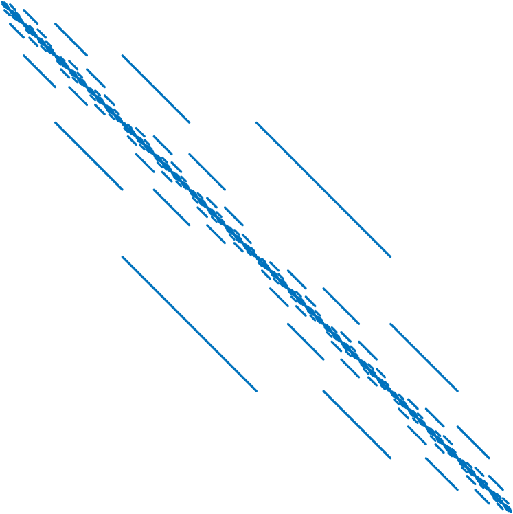
(a) Sparsity pattern of the many-body Hamiltonian.

mbl-eigvec [ width=0.95height=0.95xmin=0, xmax=184756, scaled x ticks=false, ymin=0, ymax=0.8, xtick=0,60000,120000,184756, xticklabels=0,60,000,120,000,184,756, xlabel=$i$, ylabel=$|x(i)|$, ] +[ycomb,mark=none,myblue,line width=1pt] table figs/mbl-eigvec.dat;

(b) Magnitude of each element of first eigenvector.

Figure 5: The sparsity structures of the many-body Hamiltonian associated with a Heisenberg spin chain of length 20, and its eigenvector associated with the lowest eigenvalue.

When applying the greedy algorithm (greedy-pert) to $H$, we first randomly pick 200 rows and columns of the $H$ matrix and compute the lowest eigenvalue, i.e., the ground state, and the corresponding eigenvector of $H_{1}$ using the eigs function in MATLAB, which implements the implicitly restarted Lanczos [13] or the Krylov–Schur method [28]. The choice of $200$ rows and columns is arbitrary. However, when these rows and columns are chosen randomly, the number of rows and columns has to be sufficiently large in order to prevent the greedy algorithm from converging to an undesired eigenpair. For this particular problem, 200 appears to be sufficiently large while still being relatively small compared to the dimension of $H$. We repeated the experiments multiple times with different choices of the first random 200 rows and column. All runs converge to the ground state.

We use the first order componentwise perturbation method to seek additional rows and columns of $H$ to add to the submatrix $H_{1}$ to be partially diagonalized. To be specific, we choose rows (and columns) whose corresponding $\gamma$ value defined in (9) is less than a threshold of $\tau=10^{-3}$ and add these to the submatrix $H_{1}$. We compute the lowest eigenvalue and its corresponding eigenvector of the augmented matrix again.

Then, rather than simply using the result to provide a starting guess vector for a diagonalization of the full matrix $H$, we choose to repeatedly iterate the perturbation based greedy selection process. If no additional rows (and columns) can be selected with the current threshold, we lower the threshold by a factor 10. We terminate the computation when the relative residual norm is below $10^{-7}$. Because this accuracy is already sufficient, we do not need to follow up with a calculation on the full Hamiltonian, that is, using a zero padded starting guess, as we have previously described doing at the end of the greedy selection procedure.

Table 1 shows the relative residual norm of the approximate eigenpair, $\|r\|/|\theta|$, where $r$ is is defined by (5), for each of the thresholds $\tau$ used in the greedy procedure. For each $\tau$ value, we also show the dimension of the augmented $H_{1}$ right before the threshold is lowered, and the wall clock time used to compute the desired eigenpairs for successively augmented $H_{1}$ matrices generated for that particular $\tau$ threshold.

threshold ($\tau$)	$\|r\|/|\theta|$	dim($H_{1}$)	wall clock time (sec)
$10^{-3}$	$4.7\times 10^{-3}$	$986$	$2.7\times 10^{-3}$
$10^{-4}$	$1.0\times 10^{-3}$	$2,546$	$2.9\times 10^{-3}$
$10^{-5}$	$1.7\times 10^{-4}$	$4,316$	$6.0\times 10^{-3}$
$10^{-6}$	$2.3\times 10^{-5}$	$7,558$	$8.5\times 10^{-3}$
$10^{-7}$	$3.0\times 10^{-6}$	$12,451$	$1.1\times 10^{-2}$
$10^{-8}$	$4.2\times 10^{-7}$	$18,442$	$1.7\times 10^{-2}$

Table 1: The relative residual norms of the approximate eigenpairs obtained from $H_{1}$ matrices associated with different selection thresholds $\tau$, the corresponding dimension of $H_{1}$, and the wall clock time required to compute these approximations for the Heisenberg spin-1/2 Hamiltonian with $L=20$ spins.

When the greedy algorithm terminates, the dimension of $H_{1}$ becomes 18,442, which is less than 10% of the dimension of $H$, which is 184,756 for $L=20$ spins. To illustrate the overall efficiency of this algorithm, we use the eigs function to compute the lowest eigenvalue and the corresponding eigenvector of the full $H$ directly, using a random vector as the starting guess. The total wall clock time used in this full calculation is more than seven times of that used by the greedy algorithm.

mbl-conv-size [ width=xmin=0, xmax=30, ymin=0, ymax=25000, scaled y ticks=false, xlabel=greedy iteration, title=matrix dimension $H_{1}$, legend pos=north west,legend style=draw=none,fill=none,] [GreedyResStyle] table figs/mbl-greedy-res-size.dat; [GreedyPertStyle] table figs/mbl-greedy-pert-size.dat; greedy-res,greedy-pert;

(a) The change in matrix dimension of $H_{1}$.

mbl-conv-res [ width=xmin=0, xmax=30, ymin=1e-7, ymax=1e0, xlabel=greedy iteration, title=relative residual norm, ] [black,densely dashed] coordinates(0,1e-6) (30,1e-6); [GreedyResStyle] table figs/mbl-greedy-res.dat; [GreedyPertStyle] table figs/mbl-greedy-pert.dat;

(b) The change in relative residual norm.

Figure 6: A comparison of two versions of the greedy algorithm that use different metric to select rows and columns of the disordered quantum spin chain Hamiltonian.

We then compare the perturbation analysis based greedy approach (greedy-pert) to the residual based (greedy-res) approach. Although it may be seen, in Figure 6, that the relative residual norm of the approximate eigenpairs and the dimension of the submatrix $H_{1}$ evolve similarly with the number of greedy iterations in the two approaches, the small differences in the dimension of $H_{1}$ yield slightly different time to solution.

We use the same dynamical threshold adjusting scheme to for select additional rows and columns of $H$ in the first order componentwise perturbation method.

5.3 California Road Network

In this section, we demonstrate the efficiency of the greedy algorithm when it is used to compute the principal eigenvector (PEV), i.e., the eigenvector associated with the largest (in magnitude) eigenvalue, of an adjacency matrix $H$ representing a California road network. This matrix is part of the Stanford Network Analysis Project (SNAP) collection [14] and can be download from the SuiteSparse Matrix collection [10]. The dimension of $H$ is $n=1,971,281$ and its sparsity pattern is shown in Figure 7(a). Each column (or row) of the matrix corresponds to a road intersection or endpoint which is a vertex of the corresponding adjacency graph. Each nonzero element of the matrix represents a connection between two intersections or endpoints, which constitutes an edge between two vertices on the adjacency graph. The principal eigenvector of $H$ is localized as shown in Figure 7(b). Note that each of the two peaks in Figure 7(b) actually correspond to several nonzero components of the PEV. Due to the large dimension of this matrix, the figure does not show how the nonzero elements are distributed around these two peaks. The localization of the eigenvector often indicates a densely connected subgraph. There has been a lot of effort in understanding the localization of the PEV in terms of the degrees and centralities of the nodes and structure of the graph theoretically [19, 7, 20]. The greedy algorithm provides an efficient numerical validation tool for these theoretical studies.

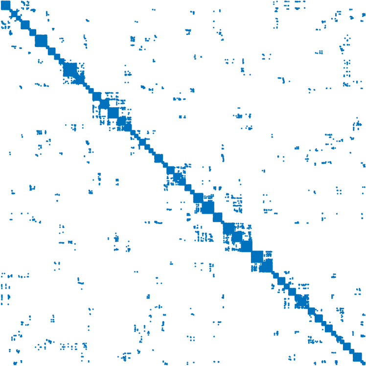
(a) The sparsity pattern of the adjacency matrix.

crn-eigvec1[spy using outlines = magnification=15,size=0.4connect spies] [ width=0.95height=0.95xmin=0, xmax=1971281, scaled x ticks=false, ymin=0, ymax=0.6, xtick=0,1000000,1971281, xticklabels=0,1,000,000,1,971,281, extra x ticks=500000,1500000, extra x tick labels=, xlabel=$i$, ylabel=$|x(i)|$, ] +[ycomb,mark=none,myblue,line width=1pt] table figs/crn-eigvec1.dat; [line width=0.1pt] coordinates (498391,0) (498391,0.002); [line width=0.1pt] coordinates (534752,0) (534752,0.002); node[fill=white] at ( 971000,0.16) 498,391; node[fill=white] at (1517000,0.16) 534,752; (spypoint) at (axis cs:517000,0.0075); (magnifyglass) at (axis cs:1250000,0.3); [spy connection path= [on background layer] [very thin,densely dotted] (tikzspyonnode.north east) – (tikzspyinnode.north east); [very thin,densely dotted] (tikzspyonnode.north west) – (tikzspyinnode.north west); [very thin,densely dotted] (tikzspyonnode.south west) – (tikzspyinnode.south west); [very thin,densely dotted] (tikzspyonnode.south east) – (tikzspyinnode.south east); ] on (spypoint) in node at (magnifyglass);

(b) Magnitude of each element of principal eigenvector.

Figure 7: The sparsity structures of the adjacency matrix associated with a California road network, and its principal eigenvector.

To compute the PEV of the adjacency matrix of the California road network, we apply the same componentwise perturbation method with an adaptively modified selection threshold that we used to compute the ground state of the MBL Hamiltonian in section 5.2 to incrementally select more rows and columns of $H$ to add to $H_{1}$. However, instead of computing the algebraically smallest eigenvalue of each submatrix identified in the greedy algorithm, here we compute the eigenvalue with the largest magnitude. Furthermore, while in the MBL problem it suffices to select a random subset of rows and columns of $H$ to construct the initial approximation to the desired eigenvalue and eigenvector, here a more careful selection of the initial approximation is needed.

Because it is believed that the nonzero components of the PEV corresponds to a densely connected subgraph of the road network graph, we first pick a row/column that has a large number of nonzeros. This row/column corresponds to the node in the network with a large degree. We then select rows and columns that correspond to nodes connected to the initially selected node with a large degree. All these selected rows and columns form our initial $H_{1}$. For the California road network, there is one node that has the highest degree of 12. There are two nodes with degree 10. All other nodes have degree less than 10.

crn-eigvec2[spy using outlines = magnification=15,size=0.2connect spies] [ width=0.475height=0.475xmin=0, xmax=1971281, scaled x ticks=false, ymin=0, ymax=0.6, xtick=0,1000000,1971281, xticklabels=0,1,000,000,1,971,281, extra x ticks=500000,1500000, extra x tick labels=, xlabel=$i$, ylabel=$|x(i)|$, ] +[ycomb,mark=none,myblue,line width=1pt] table figs/crn-eigvec2.dat; [line width=0.1pt] coordinates (562819,0) (562819,0.002); [line width=0.1pt] coordinates (577006,0) (577006,0.002); node[fill=white] at (1217000,0.16) 562,819; node[fill=white] at (1430000,0.16) 577,006; (spypoint) at (axis cs:565000,0.0075); (magnifyglass) at (axis cs:1250000,0.3); [spy connection path= [on background layer] [very thin,densely dotted] (tikzspyonnode.north east) – (tikzspyinnode.north east); [very thin,densely dotted] (tikzspyonnode.north west) – (tikzspyinnode.north west); [very thin,densely dotted] (tikzspyonnode.south west) – (tikzspyinnode.south west); [very thin,densely dotted] (tikzspyonnode.south east) – (tikzspyinnode.south east); ] on (spypoint) in node at (magnifyglass);

Figure 8: The magnitude of the eigenvector associated with the second largest (in magnitude) eigenvalue of the California road network adjacency matrix.

If we construct the initial $H_{1}$ by selecting rows and columns corresponding to the node with the maximum degree as well as all nodes connected to the maximum-degree node, which yields a $13\times 13$ matrix, the greedy algorithm converges to the second largest eigenvalue of $H$. Even though this is not the largest eigenvalue, the corresponding eigenvector, which is shown in Figure 8, is localized also with 798 large elements in magnitude. The localization region is different from the PEV shown in Figure 7(b). The subgraph containing these nodes is potentially interesting to examine also.

In order to obtain the largest eigenvalue, we select the rows/columns of the 3 nodes with degree 10 or higher, as well as all the corresponding rows/columns associated with the nodes connecting to these 3 large degree nodes up to distance 2. The dimension of this initial $H_{1}$ is $82\times 82$. Figure 9 shows how the dimension of the submatrix $H_{1}$ and the relative residual norm of the approximate eigenpair evolves with respect to the number of greedy iterations.

crn-conv-size [ width=xmin=0, xmax=20, ymin=0, ymax=1000, scaled y ticks=false, xlabel=greedy iteration, title=matrix dimension $H_{1}$, legend pos=north west,legend style=draw=none,fill=none,] [GreedyPertStyle] table figs/crn-greedy-pert-size.dat; greedy-pert;

(a) The change in matrix dimension of $H_{1}$.

crn-conv-res [ width=xmin=0, xmax=20, ymin=1e-7, ymax=1e0, xlabel=greedy iteration, title=relative residual norm, ] [black,densely dashed] coordinates(0,1e-6) (30,1e-6); [GreedyPertStyle] table figs/crn-greedy-pert.dat;

(b) The change in relative residual norm.

Figure 9: The convergence of the greedy algorithm applied to the California Road Network problem.

When the greedy algorithm terminates, the dimension of $H_{1}$ is 884, which is roughly 0.04% of the dimension of $H$. When compared to computing the PEV of $H$ directly using the eigs function, the greedy algorithm is 420 times faster in terms of wall clock time.

6 Conclusions

We presented a greedy algorithm for computing an eigenpair of a symmetric matrix $H$ that has localization properties. The key feature of the algorithm is to identify and select rows and columns of $H$ to be included in a submatrix $H_{1}$ that can be easily diagonalized (partially). The eigenvectors thus obtained for this submatrix are then used to generate more efficient starting guesses for iterative diagonalization of the full matrix $H$ if the eigenvector to be computed is not strictly localized. We discussed a number of greedy strategies and criteria for such a selection, and presented numerical examples using Hamiltonian matrices arising in two types of quantum many-body eigenvalue problems as well as an adjacency matrix describing a California road network. For all these problems, we found that the residual based selection approach is almost as good as the strategy based on perturbation analysis. Both approaches require computing $Bx_{1}$, where the submatrix $B$ is defined in (3). For large problems, accessing the entirety of $B$ may be prohibitively expensive, especially when the nonzero matrix elements of $H$ are not explicitly stored, even though this submatrix is typically sparse. Algorithms based on choosing and evaluating selected rows of $B$ will need to be developed. Similarly, it may also be prohibitively expensive to access the $C$ matrix in a full perturbation analysis. Methods for identifying good approximations to $C$ that are easy to compute also need to be developed. The efficient implementation of these algorithms is problem dependent and beyond the scope of this paper.

Even though we only showed how to compute either the smallest (algebraically) or the largest (in magnitude) eigenpair of $H$, the greedy algorithm developed here can be used to compute more than one eigenpair. If more than one eigenpair needs to be computed, the initial choice of $H_{1}$ and the subsequent selection scheme will need to take into account the presence of several eigenvectors with different localization patterns. We will investigate the practical aspects of the greedy algorithm for solving this type of problem in future work.

We should also note that there are other specialized techniques for computing localized eigenvectors and the corresponding eigenvalues in specific applications. Examples include the method based on finding a so-called landscape function and its local maximizers proposed in [1] and combinatorial approaches that can be used to identify a dense clusters or subgraph of a network [4]. The greedy algorithm proposed in this paper is not meant to replace these methods. However, it can be used to validate eigenvalues and eigenvector obtained in these methods, and is therefore a useful and complementary tool.

References

- [1] D. N. Arnold, G. David, M. Filoche, D. Jerison, and S. Mayboroda. Computing spectra without solving eigenvalue problems. SIAM J. Sci. Comput., 41(1):B69–B92, 2019. doi:10.1137/17M1156721.
- [2] D. N. Arnold, G. David, M. Filoche, D. Jerison, and S. Mayboroda. Localization of eigenfunctions via an effective potential. Commun. Partial. Differ. Equ., 44(11):1186–1216, 2019. doi:10.1080/03605302.2019.1626420.
- [3] B. R. Barrett, P. Navrátil, and J. P. Vary. Ab initio no core shell model. Prog. Part. Nucl. Phys., 69:131–181, 2013. doi:10.1016/j.ppnp.2012.10.003.
- [4] M. Charikar. Greedy approximation algorithms for finding dense components in a graph. In Proceedings of the Third International Workshop on Approximation Algorithms for Combinatorial Optimization, APPROX 2000, pages 84–95, 2000. doi:10.1007/3-540-44436-X_10.
- [5] D. Cleland, G. H. Booth, and A. Alavi. Communications: Survival of the fittest: Accelerating convergence in full configuration-interaction quantum Monte Carlo. J. Chem. Phys., 132(4):41103, 2010. doi:10.1063/1.3302277.
- [6] R. J. Harrison. Approximating full configuration interaction with selected configuration interaction and perturbation theory. J. Chem. Phys., 94(7):5021–5031, 1991. doi:10.1063/1.460537.
- [7] S. Hata and H. Nakao. Localization of Laplacian eigenvectors on random networks. Sci. Rep., 7(1):1121, 2017. doi:10.1038/s41598-017-01010-0.
- [8] A. A. Holmes, N. M. Tubman, and C. J. Umrigar. Heat-bath configuration interaction: An efficient selected configuration interaction algorithm inspired by heat-bath sampling. J. Chem. Theory Comput., 12(8):3674–3680, 2016. doi:10.1021/acs.jctc.6b00407.
- [9] A. V. Knyazev. Toward the optimal preconditioned eigensolver: Locally optimal block preconditioned conjugate gradient method. SIAM J. Sci. Comput., 23(2):517–541, 2001. doi:10.1137/S1064827500366124.
- [10] S. P. Kolodziej, M. Aznaveh, M. Bullock, J. David, T. A. Davis, M. Henderson, Y. Hu, and R. Sandstrom. The SuiteSparse Matrix Collection website interface. J. Open Source Softw., 4(35):1244, 2019. doi:10.21105/joss.01244.
- [11] A. Lagendijk, B. van Tiggelen, and D. S. Wiersma. Fifty years of Anderson localization. Phys. Today, 62(8):24–29, 2009. doi:10.1063/1.3206091.
- [12] C. Lanczos. An iteration method for the solution of the eigenvalue problem of linear differential and integral operators. J. Res. Natl. Inst. Stand. Technol., 45(4):255–282, 1950. doi:10.6028/jres.045.026.
- [13] R. B. Lehoucq, D. C. Sorensen, and C. Yang. ARPACK Users’ Guide. Society for Industrial and Applied Mathematics, 1998. doi:10.1137/1.9780898719628.
- [14] J. Leskovec, K. J. Lang, A. Dasgupta, and M. W. Mahoney. Community structure in large networks: Natural cluster sizes and the absence of large well-defined clusters. Internet Math., 6(1):29–123, 2009. doi:10.1080/15427951.2009.10129177.
- [15] Y. Li, J. Lu, and Z. Wang. Coordinatewise descent methods for leading eigenvalue problem. SIAM J. Sci. Comput., 41(4):A2681–A2716, 2019. doi:10.1137/18M1202505.
- [16] D. J. Luitz, N. Laflorencie, and F. Alet. Many-body localization edge in the random-field Heisenberg chain. Phys. Rev. B, 91(8):81103, 2015. doi:10.1103/PhysRevB.91.081103.
- [17] R. Nandkishore and D. A. Huse. Many-body localization and thermalization in quantum statistical mechanics. Annu. Rev. Condens. Matter Phys., 6(1):15–38, 2015. doi:10.1146/annurev-conmatphys-031214-014726.
- [18] C. C. Paige and M. A. Saunders. Solution of sparse indefinite systems of linear equations. SIAM J. Numer. Anal., 12(4):617–629, 1975. doi:10.1137/0712047.
- [19] R. Pastor-Satorras and C. Castellano. Eigenvector localization in real networks and its implications for epidemic spreading. J. Stat. Phys., 173(3):1110–1123, 2018. doi:10.1007/s10955-018-1970-8.
- [20] P. Pradhan, A. C.U., and S. Jalan. Principal eigenvector localization and centrality in networks: Revisited. Physica A, 554:124169, 2020. doi:10.1016/j.physa.2020.124169.
- [21] R. Roth. Importance truncation for large-scale configuration interaction approaches. Phys. Rev. C, 79(6):64324, 2009. doi:10.1103/PhysRevC.79.064324.
- [22] J. B. Schriber and F. A. Evangelista. Adaptive configuration interaction for computing challenging electronic excited states with tunable accuracy. J. Chem. Theory Comput., 13(11):5354–5366, 2017. doi:10.1021/acs.jctc.7b00725.
- [23] M. Shao, H. M. Aktulga, C. Yang, E. G. Ng, P. Maris, and J. P. Vary. Accelerating nuclear configuration interaction calculations through a preconditioned block iterative eigensolver. Comput. Phys. Commun., 222:1–13, 2018. doi:10.1016/j.cpc.2017.09.004.
- [24] S. Sharma, A. A. Holmes, G. Jeanmairet, A. Alavi, and C. J. Umrigar. Semistochastic heat-bath configuration interaction method: selected configuration interaction with semistochastic perturbation theory. J. Chem. Theory Comput., 13(4):1595–1604, 2017. doi:10.1021/acs.jctc.6b01028.
- [25] C. D. Sherrill and H. F. Schaefer. The configuration interaction method: Advances in highly correlated approaches. In Advances in Quantum Chemistry, volume 34 of Advances in Quantum Chemistry. Academic Press, 1999. doi:10.1016/S0065-3276(08)60532-8.
- [26] G. L. G. Sleijpen and H. A. Van der Vorst. A Jacobi–Davidson iteration method for linear eigenvalue problems. SIAM Rev., 42(2):267–293, 2000. doi:10.1137/S0036144599363084.
- [27] P. Sternberg, E. G. Ng, C. Yang, P. Maris, J. P. Vary, M. Sosonkina, and H. V. Le. Accelerating configuration interaction calculations for nuclear structure. In SC ’08: Proceedings of the 2008 ACM/IEEE Conference on Supercomputing, pages 1–12, 2008. doi:10.1109/SC.2008.5220090.
- [28] G. W. Stewart. A Krylov–Schur algorithm for large eigenproblems. SIAM J. Matrix Anal. Appl., 23(3):601–614, 2002. doi:10.1137/S0895479800371529.
- [29] J. Suhonen. From Nucleons to Nucleus. Theoretical and Mathematical Physics. Springer-Verlag, Berlin, Heidelberg, 2007. doi:10.1007/978-3-540-48861-3.
- [30] N. M. Tubman, J. Lee, T. Y. Takeshita, M. Head-Gordon, and K. B. Whaley. A deterministic alternative to the full configuration interaction quantum Monte Carlo method. J. Chem. Phys., 145(4):44112, 2016. doi:10.1063/1.4955109.
- [31] R. Van Beeumen, G. D. Kahanamoku-Meyer, N. Y. Yao, and C. Yang. A scalable matrix-free iterative eigensolver for studying many-body localization. In Proceedings of the International Conference on High Performance Computing in Asia-Pacific Region, HPCAsia2020, pages 179–187, 2020. doi:10.1145/3368474.3368497.
- [32] Z. Wang, Y. Li, and J. Lu. Coordinate descent full configuration interaction. J. Chem. Theory Comput., 15(6):3558–3569, 2019. doi:10.1021/acs.jctc.9b00138.
- [33] H. Zou, T. Hastie, and R. Tibshirani. Sparse principal component analysis. J. Comput. Graph. Statist., 15(2):265–286, 2006. doi:10.1198/106186006X113430.