Maximum Entropy Models from Phase Harmonic Covariances
Abstract
The covariance of a stationary process is diagonalized by a Fourier transform. It does not take into account the complex Fourier phase and defines Gaussian maximum entropy models. We introduce a general family of phase harmonic covariance moments, which rely on complex phases to capture non-Gaussian properties. They are defined as the covariance of , where is a complex linear operator and is a non-linear phase harmonic operator which multiplies the phase of each complex coefficient by integers. The operator can also be calculated from rectifiers, which relates to neural network coefficients. If is a Fourier transform then the covariance is a sparse matrix whose non-zero off-diagonal coefficients capture dependencies between frequencies. These coefficients have similarities with high order moment, but smaller statistical variabilities because is Lipschitz. If is a complex wavelet transform then off-diagonal coefficients reveal dependencies across scales, which specify the geometry of local coherent structures. We introduce maximum entropy models conditioned by these wavelet phase harmonic covariances. The precision of these models is numerically evaluated to synthesize images of turbulent flows and other stationary processes.
Keywords— covariance, stationary process, phase, Fourier, wavelets, turbulence
1 Introduction
Many phenomena in physics, finance, signal processing and image analysis can be modeled as realizations of a non-Gaussian stationary process . We often observe a single realization of dimension from which the model must be estimated. Models of stochastic processes may be defined as maximum entropy distributions conditioned by a predefined family of moments [1, 2]. To estimate accurately these moments from a single or few realizations, the number of moments should not be too large. The Fourier transform diagonalizes the covariance of stationary processes but a maximum entropy model conditioned by these second order moments is Gaussian. The main difficulty is to specify moments which characterize important classes of non-Gaussian stationary distributions.
Second order moments do not depend upon the complex phase of Fourier coefficients. We shall see that this complex phase plays a crucial role to specify non Gaussian properties of probability distributions, which can be captured with appropriate covariance moments. We define a phase harmonic covariances as the covariance of , where is a complex linear operator and is a non-linear phase harmonic operator introduced in [3]. The operator multiplies by integers the phase of each complex coefficient of . The paper studies general properties of phase harmonic covariances when is a Fourier or a wavelet transform, to approximate non-Gaussian distributions through maximum entropy models.
If is a Fourier transform, Section 2 proves that the covariance of is a sparse matrix whose non-zero off-diagonal coefficients reveal non-linear dependencies between different frequencies. Similarly to high order moments, the covariance of captures this dependence across frequencies by cancelling relative phase fluctuations. A high order moment of a complex random variable computes an exponentiation , which amplifies the variability of large if . A phase harmonic operator performs a similar transformation of the phase by calculating . It also produces non-zero off-diagonal covariance coefficients without amplifying . It is a Lipschitz operator as opposed to high order exponentiations, which reduces the variance of empirical statistical estimators.
The error of a maximum entropy model can be measured with a Kullback-Leibler divergence relatively to the true probability distribution of . Section 2.1 explains that this error can be reduced by improving the sparsity of . For large classes of random processes , sparsity is improved by defining as a complex wavelet transform as opposed to a Fourier transform. High order moments of wavelet coefficients have been used to characterize non-Gaussian multifractal properties of random processes and turbulent flows [4, 5]. We replace these high order moments by the covariance matrix of , to capture non-linear dependencies across scales, without suffering from high statistical variabilities. Dependencies across scales reveal the existence of coherent signal structures as opposed to Gaussian fluctuations. Section 3 studies the covariance of this wavelet phase harmonic operator.
Wavelet phase harmonics are related to the pioneer work of Grossmann and Morlet [6], who showed qualitatively that complex wavelet transforms have a phase whose variations across scales provide important information on the geometry of transient structures. In image processing, Portilla and Simoncelli [7] brought a new perspective by showing that one can synthesize non-Gaussian image textures from the covariance of the modulus of wavelet coefficients and by using their phase at different scales. We shall see that Portilla and Simoncelli covariances coefficients [7] are low order phase harmonic covariances , computed with a wavelet transform . Other remarkable image texture syntheses have been obtained in [8], by computing the covariance of output coefficients of an one-layer convolutional neural network with a rectifier. Section 3.2 proves that a non-linear phase harmonic operator can be calculated with a rectifier followed by a Fourier transform along a phase variable. These neural network covariances are therefore equivalent to phase harmonic covariances, but for a convolutional operator which is not a wavelet transform. The analysis of phase harmonic operators and the properties of covariance matrices gives a general mathematical framework to understand these algorithms. It guides the choice of the linear transform , of the diagonal and off-diagonal covariance moments, to model specific classes of random processes.
Section 4 reviews the properties of maximum entropy models conditioned by empirical estimators of covariance moments. Sampling a maximum entropy distribution requires to use expensive algorithms that iterate over Gibbs samplers [9], which is not feasible over large size images. We thus rather use microcanonical models studied in [10]. Samples of microcanonical models are estimated by transporting an initial maximum entropy measure with a gradient descent which adjusts its moments. Section 5 defines low-dimensional foveal models conditioned by a small subset of wavelet phase harmonics covariances. These moments capture local dependencies within and across scales. We evaluate the numerical precision of foveal wavelet phase harmonic models, to approximate two-dimensional non-Gaussian processes including images of turbulent flows and multifractals. All calculations can be reproduced by a Python software available at https://github.com/kymatio/phaseharmonics.
Notations: We write the complex conjugate of , is the complex transpose of a matrix and is the adjoint of an operator . The covariance of two random variables and is written . An inner product is written in and in . The cardinal of a set is . The norm of in or is written .
2 Fourier Phase Harmonic Representation
Section 2.1 introduces general properties of maximum entropy models conditioned by covariance coefficients of a non-linear representation over a graph. Section 2.2 then shows that the Fourier coefficients of a stationary process are uncorrelated because of phase fluctuations. It motivates the use of higher order moments to define a representation which can cancel random phase fluctuations and capture dependence across frequencies. Section 2.3 reviews the properties of phase harmonic operators introduced in [3]. If is a Fourier transform, Section 2.4 shows that is a bi-Lipschitz representation, whose covariance captures non-Gaussian properties through dependencies across frequencies, similarly to high order moments.
2.1 Maximum Entropy Covariance Graph Models
We introduce maximum entropy models of a stationary random vector , conditioned by covariance coefficients of a representation which is also a random vector:
with . We suppose that is defined for in a cube with grid points, for example in . If then each realization is an image of pixels. This section reviews general properties of maximum entropy models defined on a graph, which take advantage of known symmetries of the distribution of .
Maximum entropy on a graph with symmetries
Let us write , where and is a finite set of vertices in a graph that we shall define. The representation is a complex-valued vector in .
We introduce a maximum entropy model conditioned by the covariance between vertices
where is in a neighborhood of . We suppose that . If then so it defines a reflexive and symmetric undirected graph , where the set of edges relates all neighbors . The edge weights are the covariances over . In statistical physics, is called the interaction potential of , where the mean is considered here as a predefined constant vector.
Let be the probability density of . We can reduce the constraints of the maximum entropy model if we also know a finite group of symmetries of . We consider linear unitary symmetries from to , which satisfy for all . The stationarity of in means that is invariant to periodic translations, that we write , so includes all translations. If is invariant to rotations then also includes rotations. Since is invariant to the action of , its covariance is also invariant to the action of any
Let be the total number of symmetries. These conditions will be included in the maximum entropy model.
The entropy of a density on is
A maximum entropy macrocanonical model conditioned by the covariance over and by the symmetry group has a probability density which maximizes and satisfies covariance moment conditions for all
| (1) |
If there exist Lagrange multipliers such that
| (2) |
is a probability distribution which satisfies each equality constraint (1), then it is the unique solution to the maximum-entropy problem [2]. The sum in the exponential is the Gibbs energy, and is the partition function. Since we have . We verify that for all , so is also a group of symmetries of . If includes all translations then is stationary.
In the particular case where all are linear operators then the Gibbs energy is bilinear and is thus a Gaussian distribution. Appendix A shows that the Lagrange multipliers can then be computed efficiently [2]. If some of the are non-linear then computing the Lagrange multipliers is computationally very expensive when the dimension of and the total number of moments is large.
Covariance estimation from symmetries
The covariance estimation from a single realization of is calculated with an average over the symmetries of . The orbit of the action of on is the set of . The empirical estimation of is computed as an empirical average over this orbit
| (3) |
Similarly, is estimated with an average on the same orbit
| (4) |
Summing over all transformations of by is called “data augmentation” in machine learning. The larger the more accurate the estimation. The maximum entropy model is estimated from a single realization by replacing the mean and covariance in (1) by their estimation and .
The existence of symmetries also reduces the number of covariances that must to be estimated. We define as a minimum set of edges such that for any there exists such that and . Since is invariant to the action of , its covariance is also invariant:
It is therefore sufficient to estimate covariance coefficients indexed by to specify all covariances indexed by . The set is interpreted as a set of sufficient statistics. Given a realization of dimension , to control the overall covariance estimation errors we must insure that .
Bi-Lipschitz continuity
The estimation of covariance coefficients may have a large variance in the presence of rare outliers. These outliers induce a large variability in the empirical sum (4) depending upon the realization of . To avoid amplifying these outliers, we impose that is bi-Lipschitz, so that the variations of are of the same order as the variations of . It also insures that is an invertible operator.
The representation is bi-Lipschitz if there exists and such that for all
| (5) |
For any random vector , we write , which is the trace of its covariance. The following proposition proves that the variance of and have the same order of magnitude.
Proposition 2.1.
If is bi-Lipschitz then
| (6) |
Proof: If and are two independent random vectors having same probability distribution then the bi-Lipschitz bounds (5) of imply that
| (7) |
If and are two i.i.d random variables then we verify that
where the first expected value is taken relatively to the joint distribution of and . It results that and . Inserting these equalities in (7) proves (6).
Maximum entropy reduction with sparsity
Zhu, Wu and Mumford [11] have proposed to optimize maximum entropy parameterized models by minimizing the resulting maximum entropy. Indeed, if has a probability density then model error can be evaluated with a Kullback-Leibler divergence
We verify that by inserting (2) and by using the equalities (1). Since , it results that the Kullback-Leibler divergence is equal to the excess of entropy of the maximum entropy model:
| (8) |
We thus reduce the model error by reducing the maximum entropy to obtain a lower entropy model. The minimum is reached if and only if almost-surely.
In our case, the model depends upon the choice of and of the edges of the covariance graph. Optimizing by calculating is computationally too expensive. However, we explain below that we can minimize an upper bound of by finding a representation such that is as sparse as possible, which gives a partial control on the maximum entropy. Let be a maximum entropy model of density . If has a stable inverse, which we guarantee with the bi-Lipschitz condition, then an upper bound of can be computed from the entropy of each marginal . Such an entropy is small if is sparse, because it then has a narrow probability density centered at . To impose this sparsity we must find a representation such that is sparse. This sparsity must also be captured by diagonal covariance coefficients so that the maximum entropy model , conditioned by these moments retains this sparsity. This is the case for Fourier and wavelet phase harmonic representations studied in Sections 2.4 and 3.2. For non-Gaussian processes, it amounts to represent “coherent structures” with as few non-zero coefficients as possible.
Increasing the number of moment conditions can further reduce but it also increases the statistical error when estimating these moments from a single realization of . The choice of is thus a trade-off between the model error (bias) and the estimation error (variance).
2.2 Fourier Phase and High Order Moments
The covariance of a stationary random vector is diagonalized by the discrete Fourier transform, because of random phase fluctuations. This suggests defining a covariance representation in a Fourier basis. For non-Gaussian processes, the dependence of Fourier coefficients is partly captured by high order moments which cancel random phase fluctuations.
For , since for is stationary, only depends on . We write the norm of and the inner product. A low-dimensional maximum entropy model is constructed on by restricting covariances to neighborhoods of fixed radius: . The radius is chosen to be large enough to capture long range correlations. Since is stationary, the symmetry group includes translations and we can thus define by setting . The maximum entropy model then defines a Gauss-Markov random vector [2] specified by covariances in a small neighborhood. This model does not capture non-Gaussian properties. If is an r-dimensional grid, then the model size is . It may be large if the process has long-range spatial correlations.
To better understand how to capture non-Gaussian properties, we study these covariance coefficients in a Fourier basis. We write the discrete Fourier transform of over :
| (9) |
The Fourier representation is indexed by . The covariance for is
If then . If then because of random phase fluctuations. Indeed, translating by any multiplies by . Since is stationary, this translation is a symmetry which does not modify . It results that
| (10) |
Since this is true for any it implies that
| (11) |
Since the discrete Fourier transform is periodic beyond , any equality or non-equality between frequencies must be understood modulo along the directions. If is Gaussian then is also Gaussian so this non-correlation implies that and are independent. However, if is non-Gaussian then and are typically not independent.
Phase cancellation with higher order moments
To capture the dependencies of Fourier coefficients across frequencies, one can use high order moments [12]. For any , similarly to (10), translating by yields
| (12) |
A high-order Fourier representation is indexed by with . It results from (12) that
| (13) |
If and is not Gaussian then this covariance is typically non-zero because the phase variations of cancel the phase variations of . This is also the key idea behind the use of bi-spectrum moments [13]. By adjusting these moments provide some dependency information between and for .
For example, let be a random shift vector, where is a fixed signal supported in and is a random periodic shift which is uniformly distributed in . It is a stationary process whose Fourier coefficients have a random phase: . In this case, if then
It is non-zero at frequencies where does not vanish. This shows that covariances of the high order Fourier exponents can capture the dependence of Fourier coefficients at different frequencies. However, this high order Fourier representation is not Lipschitz. Indeed, when , the exponent amplifies the variability of each random variables , so estimators of covariance coefficients have a large variance.
2.3 Phase Harmonic Operator
We review the properties of phase harmonic operators introduced in [3], which replace high order exponents by an exponent on the phase only. These operators are bi-Lipschitz and can be computed by applying a rectifier followed by a Fourier transform on a phase variable. If is a Fourier tranform, next section shows that can have non-zero covariance coefficients across frequencies because of relative phase cancellations.
If then . If then amplifies large values of and hence the variance of a random variable . A phase harmonic computes a power of the phase only:
It preserves the modulus: . A phase harmonic operator computes all such phase harmonics
| (14) |
with finite energy weights . The harmonic weights amplify or eliminate different phase harmonics.
Phase windows and phase Fourier transform
We show that is the Fourier transform along a phase variable of a non-linear phase windowing operator, which can be computed with rectifiers used in neural networks.
Let us write the Fourier transform along phases:
| (15) |
Observe that . It results that
with
| (16) |
The operator translates the phase of by and applies a periodic phase windowing .
A rectifier is an important example of non-linearity which acts as a phase windowing when applied on the real part of . Indeed
so
| (17) |
The rectifier phase window is positive and supported in . The corresponding harmonic weights are computed in [3] with the Fourier integral (15):
| (18) |
Their decay is slow because has discontinuous derivatives at .
Bi-Lipschitz continuity
We mentioned that polynomial exponents amplify the variability of random variables around their mean. Indeed if then may be arbitrarily large if . On the contrary, a phase harmonic preserves the modulus which provides a bound on such amplification. It is proved in [3] that it is Lipschitz continuous
| (19) |
The distance is therefore amplified by at most .
This Lipschitz continuity is extended to phase windowed Fourier transforms, which are shown to be bi-Lipschitz. The Fourier transform preserves norms and distances. Calculating the norm of (14) gives
with . Following [3], we also derive from (19) that a phase windowed Fourier transform is bi-Lipschitz over complex numbers
| (20) |
with and . The upper bound is derived from (19) and the lower bound is obtained isolating the terms corresponding to . For the rectifier filter (18), we get and . The following theorem gives a tight upper Lipschitz constant for the rectifier filter, proved in Appendix B.
Theorem 2.1.
The rectifier phase window has a Lipschitz upper-bound .
2.4 Phase Harmonics of Fourier Coefficients
If computes the Fourier transform of then the resulting phase harmonic representation is
It is indexed by . We show that the covariance of is sparse but not necessarily diagonal. Section 2.2 explains that if is stationary then and are not correlated if but and may be correlated if is not Gaussian. Similarly we show that the covariance of and may become non-zero for , which reveals non-Gaussian properties.
Since is bi-Lipschitz and the Fourier transform is unitary up to a factor , it results that is bi-Lipschitz with Lipschitz constants and . Proposition 2.1 implies that
| (21) |
Sparse phase harmonic covariance
Phase harmonic covariance coefficients are
If is compactly supported in , since is of dimension , the covariance has coefficients. The following proposition proves that coefficients of are mostly zero and it is diagonal if is Gaussian. Diagonal values are specified.
Theorem 2.2.
If is real stationary then
| (22) |
Along the diagonal, if and or if and is odd then
| (23) |
If and is even then
| (24) |
For all
| (25) |
If is Gaussian then is diagonal and if .
The proof is in Appendix C. All equalities or non-equalities on frequencies must be understood modulo in dimension . Property (22) proves that is highly sparse. If is not Gaussian then off-diagonal coefficients are typically not zero when . For , we get modulus covariances which are a priori non-zero for all . It provides no information on the phase of and . Phase correlations are captured when . If , it results from (22) that only if is colinear with . For a grid of size , there are such frequencies . The total number of non-zero off-diagonal covariance coefficients is thus at most .
For a non-Gaussian process, off-diagonal coefficients with are typically non-zero. This is illustrated with a random shift process where is uniformly distributed in . If then one can verify that
If does not vanish then all these coefficients are non-zero.
Along the diagonal, (23) and (24) prove that all coefficients are either equal to or to . Property (25) also proves that the ratio between these covariance values depend upon the ratio . This ratio measures the sparsity of multiple realizations of the random variable . Indeed, expected values are estimated by normalized sums, so ratio of expected values can be interpreted as ratios of over norms, which is a measure or sparsity. For all Gaussian random variables, this ratio is equal to . If the ratio is smaller than then has a high probability to be relatively small and it has large amplitude outliers of low probability. The probability distribution of is then highly peaked in zero with a long tail. The smaller this ratio the lower the entropy of this marginal probability distribution.
We saw in (8) that a maximum entropy model introduces errors if its entropy is much larger than the entropy of . The entropy is bounded by the sum of the entropy of each random variable , which is conditioned by and . It gives an upper bound on the entropy , which decreases if the sparsity of increases. However, if has sharp localized transitions then its Fourier coefficients have typically a large amplitude across most frequencies and are not sparse. On the contrary, wavelet coefficients may be sparse. In this case, we shall capture this sparsity and thus compute maximum entropy models of lower entropy, by replacing the Fourier transform by a wavelet transform.
3 Wavelet Phase Harmonics
To model random vectors whose realizations include singularities and sharp transitions, we define a phase harmonic representation where is a wavelet transform as opposed to a Fourier transform. Indeed, wavelet transform provides sparse representations of such signals and Section 2.1 explains that imposing sparsity constraints typically improves the accuracy of maximum entropy models. We concentrate on two-dimensional image applications. The same approach applies to signals of any dimension, with an appropriate wavelet transform. Section 3.1 reviews the construction of complex steerable wavelet frames and the properties of their covariance matrices. Section 3.2 studies the covariance of wavelet phase harmonics.
3.1 Steerable Wavelet Frame Covariance
Complex steerable wavelet frames were introduced in [14] and are further studied in [15], to easily compute wavelet coefficients of rotated images. For simplicity, we begin by introducing wavelets as a localized functions for , with . Complex steerable wavelets have a Fourier concentrated over one-half of the Fourier domain. We impose that so that is real. This Fourier transform is centered at a frequency and is non negligible for such that for some . Figure 1 gives an example of such a wavelet, which is specified in Appendix D.
Let be a rotation by an angle . Multiscale steerable wavelets are derived from with dilations by for , and rotations over angles for
| (26) |
Since is non negligible for it results that is centered at and non negligible for . In space, is non-negligible for . We limit the scale to a maximum . The lowest frequencies are captured by a wavelet centered at . It is computed by dilating a function such that :
| (27) |
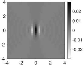
A wavelet frame is constructed by translating each for by and by for all . It introduces a factor oversampling relatively to a wavelet orthonormal basis [16], which creates some redundancy. The wavelet transform of is defined by
where is a frequency-space index set with for , , , or .
Under appropriate conditions on , the wavelet family is a frame of [15]. This means that there exists such that for any
| (28) |
with .
The wavelet transform can be redefined over discrete images of pixels supported in a two-dimensional square grid , uniformly sampled at intervals in . It requires to discretize and modify “boundary wavelets” whose supports intersect image boundaries. This can be done over steerable wavelets [14, 15], while preserving the frame constants and . The resulting wavelet are supported in . They are still indexed by . If for , then . If then . Since , there are at most different frequency channels . For , is translated by which yields wavelet coefficients. The total number of wavelets coefficients is about if .
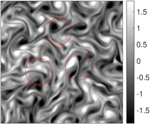
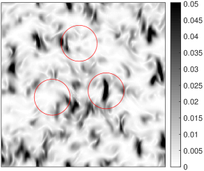
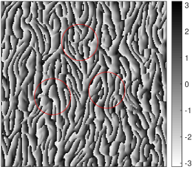
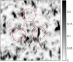
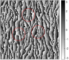
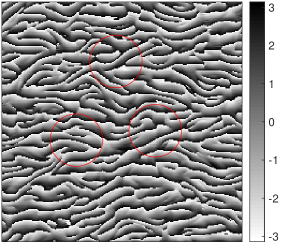
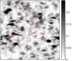
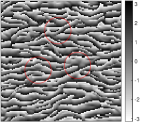
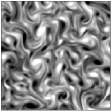
The mother wavelet is chosen in order to obtain a sparse wavelet representation of realizations of , with few large amplitude wavelet coefficients. This sparsity highlights non-Gaussian properties. Figure 2 displays the modulus and phase of wavelet coefficients of the vorticity field of a turbulent flow. This flow is obtained by running the 2D Navier Stokes equation with periodic boundary conditions, initialized with a random Gaussian field [17]. After a fixed time, it defines a stationary but non-Gaussian random process. For each scale and orientation, large amplitude modulus coefficients are located at positions where the image has sharp transitions, and the phase depends upon the position of these sharp transitions.



Wavelet covariance
A wavelet transform defines a linear representation indexed by . Similarly to Fourier coefficients, we show that wavelet coefficients have a covariance which nearly vanish at different frequencies.
Similarly to Fourier coefficients, wavelet coefficients have a zero mean at non-zero frequencies. If then because . If then so . The covariance at and is
It depends on because is stationary. Let be the discrete Fourier transform of defined in (9). Since wavelet coefficients are convolutions, covariance values can be rewritten from the power spectrum of
| (29) |
It results that if for all . Since is non-negligible only if , the covariance is non-negligible for only if
| (30) |
It shows that similarly to Fourier coefficients, wavelet covariances are negligible across frequencies which are sufficiently far apart.
Maximum entropy wavelet graph model
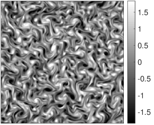
A maximum entropy model conditioned by wavelet covariances is Gaussian because the wavelet transform is linear. Figure 3(a) gives a realization of a stationary turbulent flow . A low-dimensional maximum entropy model is defined on a graph of covariance coefficients for in a small neighborhood of . Since wavelet coefficients are nearly decorrelated across frequencies, at each scale , the neighborhood of is defined as the set of such that and for a fixed . Covariances are thus specified over a spatial range proportional to the scale. This is a foveal neighborhood which is sufficient to approximate the covariances of large classes of random processes such as fractional Brownian motions [18]. Since , the neighborhoods of all have the same size, which is smaller than .
Since is stationary, its probability distribution is invariant to the group of translations. The number of covariance coefficients that must be estimated is equal to the number of edges in the graph modulo translations. It is equal to the number of wavelet frequencies multiplied by the size of each neighborhood, and thus bounded by . This model size is much smaller than the image size when is large.
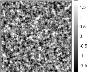
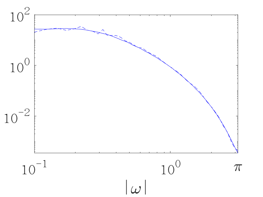
Figure 3(b) shows a realization of the maximum entropy Gaussian model . It is conditioned by wavelet covariances on a foveal graph with . The wavelet transform is computed with a bump wavelet specified in Appendix D, with , and . In this case . The covariances are estimated from a single realization of . The calculation of the Lagrange multipliers in (2) is explained in Appendix A. To measure the accuracy of this model we compare the power spectrum of and the Gaussian model . Both processes are isotropic so Figure 3(c) gives the radial log power spectrum of and as a function of . These power spectrum are nearly the same, which means that the wavelet covariance graph gives an accurate estimation of the second order moments of from a single realization.
The realization of the Gaussian model in Figure 3(b) has a geometry which is very different from the turbulence flow in Figure 3(a). It shows that is highly non-Gaussian, which also appears in Figure 2. The wavelet coefficients of a stationary process are not correlated at different scales and angles, which would imply that they are independent if was Gaussian. On the contrary, Figure 2 shows that the the modulus and phases of wavelet coefficients of are strongly dependent across scales and angles. High amplitude modulus coefficients are located in the same spatial neighborhoods because they are produced by the same sharp transitions of the flow. Next section explains how to capture this dependence with phase harmonics.
3.2 Wavelet Phase Harmonic Covariance
A wavelet phase harmonic representation is computed with a linear wavelet transform . As in the Fourier case, the covariance of has non-zero covariance coefficients across different frequency bands. We study the properties of the resulting covariance matrix, and the role of sparsity.
Wavelet phase harmonics
To specify the dependence across frequencies, we apply a phase harmonic operator to wavelet coefficients:
The coefficients of are indexed by . The covariance coefficients of are
Since is stationary, it only depends on . Wavelet harmonic covariances only need to be calculated for and . Indeed, since is real and one can verify that does not change its value if becomes or if becomes . Such wavelet harmonic covariances have first been computed by Portilla and Simoncelli [7] to characterize the statistics of image textures. Their representation correspond to equal to , , , which amounts to choosing .
Since and are bi-Lipschitz the operator is also bi-Lipschitz, with lower and upper bounds and . Proposition 2.1 implies that
| (31) |
which controls the variance of wavelet harmonic coefficients.
Rectified neural network coefficients
Ustyuzhaninov et. al. in [8] have shown that one can get good texture synthesis from the covariance of a one-layer convolutional neural network, computed with a rectifier. In the following we show that these statistics are equivalent to phase harmonic covariances, computed with a rectifier phase window .
Section 2.3 proves that , where computes a phase windowing of wavelet coefficients
The covariance of and thus satisfy . The following proposition proves that gives the covariance of rectified wavelet coefficients if is a rectifier phase window.
Proposition 3.1.
Let and . For a rectifier phase window
| (32) |
with .
Rectified wavelet coefficients can be interpreted as one-layer convolutional network coefficients, computed with wavelet filters of different frequencies and different phases . This result applies to any linear operator , not necessarily a wavelet transform. The statistics used by Ustyuzhaninov et. al. in [8] use local cosine or random filters in their network as opposed to steerable wavelets. It corresponds to convolutional operators that are not wavelet transforms.
Sparse harmonic covariance
Proposition 2.2 specifies the properties of a Fourier phase harmonic covariance. We qualitatively explain, without proof, why has similar sparsity properties.
For a fixed and , is a stationary random vector in . The covariance of and is non-zero only if their power-spectrum have a support which overlap. We give a necessary condition by approximating these spectrum supports.
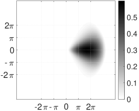
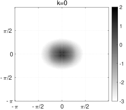
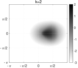
For , the spectrum of has an energy concentrated at frequencies where the Fourier transform of is concentrated, which is included in a ball centered at of radius . For , [3] explains that the Fourier transform of and hence its power spectrum is concentrated in a ball centered at of radius . If then the spectrum of is concentrated in a ball centered at the frequency, of radius . This is illustrated numerically in Figure 4 which displays the power spectrum of for . In this case, is a stationary vorticity field shown at the top of Figure 3(a). These power spectrum are estimated for a fixed from independent realizations of . For , the power spectrum is supported over the Fourier support of . For its support is approximately dilated by , whereas for it is centered at the zero frequency.
It results that the spectrum of and have a support which overlap only if
| (33) |
Similarly to the Fourier case, if then this condition is satisfied for any pair of frequencies . It corresponds to covariances of modulus coefficients , which are typically non-zero when the process is non-Gaussian.
If and then non-negligible values of occur for . This is similar to the vanishing property (22) of Fourier harmonic coefficients, at frequencies which are colinear. Since and , it requires that and that .
Diagonal covariance coefficients have similar properties as Fourier coefficients. They are specified by and , which do not depend upon . Moreover when ,
The ratio measures the sparsity of wavelet coefficients . Indeed, the sparsity of a time series is usually quantified by its norm for a fixed norm [16], which amounts to compute their ratios. Since is stationary, spatial sums over converge to expected values. It results that a ratio of an over an norm is an estimator of the ratio of expected values. If is Gaussian then is a complex Gaussian random variable and one can verify that this ratio is for all . A ratio smaller than implies that wavelet coefficients are sparse and hence that is non-Gaussian.
To increase the accuracy of a maximum entropy model , the Kullback-Leibler divergence (8) shows that we must minimize its entropy. As in the Fourier case, an upper bound of the entropy is obtained as a sum of the entropy of the marginals of wavelet coefficients. The marginal entropies get smaller by reducing the sparsity ratio . To minimize this upper bound of the model entropy, this suggests by finding a mother wavelet which yields sparse coefficients.
Gaussianity test
Even though and may have disjoint Fourier supports, the previous analysis showed that one can find and such that the spectrum of and overlap, for example with . A priori, the covariance is then non-zero, unless is Gaussian in which case these coefficients vanish, as proved by the following theorem.
Proposition 3.2.
Let be such that . If is Gaussian and stationary then if and , for any .
Proof: If is Gaussian then and are jointly Gaussian random variables. Equation (29) proves that if then . These Gaussian random variables are uncorrelated and therefore independent. It results that and are also independent and thus have a covariance which is zero.
This proposition gives a test of Gaussianity by considering two frequencies and where is sufficiently large so that the support of and do not overlap. If then wavelet harmonic covariances are zero if is Gaussian but it is typically non-zero if is not Gaussian.
4 Microcanonical Models
Section 2.1 introduces macrocanonical maximum entropy models conditioned by covariance coefficients of a representation . The resulting maximum entropy distribution depend upon Lagrange coefficients which are computationally very expensive to calculate, despite the development of efficient algorithms [19]. Section 4.1 reviews maximum entropy microcanonical models which avoid computing these Lagrange multipliers. Section 4.2 gives an alternative microcanonical model which is calculated with a faster algorithm, which transports a maximum entropy measure by gradient descent.
4.1 Maximum Entropy Microcanonical Models
Microcanonical models avoid the calculation of Lagrange multipliers and are guaranteed to exist as opposed to macrocanonical models. We first specify covariance estimators and then briefly review the properties of these microcanonical models.
Microcanonical models rely on an ergodicity property which insures that covariance estimations concentrate near the true covariance when is sufficiently large. Let be a known group of linear unitary symmetries of the density of . It includes translations because is stationary. An estimation of the covariance over the edge set is computed in (4) from a single realization of , by transforming with all . To differentiate realizations of from other , we associate a similar covariance estimation to any . This covariance is centered on the empirical mean computed in (3) and defined by
| (34) |
It is invariant to the action of any on .
We denote . We shall suppose that satisfies the following covariance ergodicity property over :
| (35) |
To satisfy this property the number of covariance moments must be small compared to the dimension of . The ergodicity hypothesis implies that when is sufficiently large, with high probability, the empirical covariance of a realization of is close to the true covariance over .
Given a realization of , a microcanonical set of width is the set of all which have nearly the same covariance estimations as :
| (36) |
A maximum entropy microcanonical model has a probability distribution of maximum entropy supported in . The set is bounded. Indeed, if then . Since includes all diagonal coefficients for , one can derive an upper bound for . Since is bi-Lipschitz, we also obtain an upper bound for . Since , the Lebesgue measure of is non-zero, therefore the maximum entropy distribution is uniform in relatively to the Lebesgue measure. A major issue in statistical physics is to find sufficient conditions to prove the Boltzmann equivalence principle which guarantees the convergence of microcanonical and macrocanonical models towards the same Gibbs measures when goes to [20]. This involves the proof of a large deviation principle which expresses concentration properties of the covariance of . If is continuous and bounded so that the interaction potential is also continuous and bounded, and if there is no phase transition, which means that the limit is a unique Gibbs measure, then one can prove that microcanonical and macrocanonical measures converge to the same limit for an appropriate topology [21, 22]. The bounded hypothesis is not necessary and may not be satisfied.
The ergodicity property (35) guarantees that concentrates in with a high probability when is sufficiently large. The microcanonical set may however be much larger than the set where concentrates, which means that the maximum entropy microcanonical distribution may have a much larger entropy than the entropy of . As in the macrocanonical case, the representation must be optimized in order to reduce the maximum entropy, which motives the use of sparse representations.
4.2 Gradient-Descent Microcanonical Models
Sampling a maximum entropy microcanonical set requires to use Monte Carlo algorithms. They are computationally very expensive when the number of moments and the dimension are large, because their mixing time become prohibitive [23]. Following the approach in [10], we approximate these microcanonical models with a gradient descent algorithm.
Gradient-descent microcanonical models are computed by transporting an initial Gaussian white noise measure into the microcanonical set . This transport is calculated with a gradient descent which progressively minimizes
| (37) |
with a sufficiently large number of iterations so that and hence .
The initial Gaussian white noise is a maximum entropy distribution conditioned by a variance . This variance is chosen to be an upper bound of the empirical variance of along , calculated from diagonal coefficients of . It guarantees that the resulting white noise has an entropy larger than the microcanonical model. The gradient descent progressively reduces this entropy while transporting the measure towards . Entropy reduction bounds are computed in [10].
The initial is Gaussian white noise. For all , the gradient descent iteratively computes
This operation transports the probability measure of into a measure of . We stop the algorithm at a time which is large enough so that with a high probability. Since is not convex, there is no guarantee that even for large . In numerical calculations in Section 5, we may use several initializations, typically , to evaluate the model. The differentiability of relies on the smoothness of the function , which is differentiable at . The implementation uses an analytic formula of its derivative at and applies the same formula at .
The empirical covariance is computed in (34) with an average over all symmetries of a known group of linear unitary operators in . The following theorem proves that is also a group of symmetries of the probability measures obtained by gradient descent.
Theorem 4.1.
For any , the probability measure of is invariant to the action of .
The proof is in Appendix E. It is a minor modification of the proof in [10]. We replace the gradient descent method by L-BFGS algorithm with line search [24]. It has a faster and more accurate numerical convergence. Since includes translations, this theorem implies that each is stationary. It is shown in [10] that the transported density supported in may be different from the maximum entropy density in because the gradient descent reduces too much the entropy. In general, the precision of these microcanonical gradient descent models are not well understood. However, this theorem proves that the gradient descent preserves all known symmetries of the distribution of , which is also true for a maximum entropy measure. The sampling algorithm in [7] is different since it relies on iterative gradient projections for to satisfy constraints of various nature, which is not guaranteed to preserve symmetries.
The gradient descent may converge faster by preconditioning . This is done by replacing estimated covariances by normalized correlation coefficients
| (38) |
Any is a symmetry of and is therefore a symmetry of normalized correlation coefficients, so Theorem 4.1 remains valid with this preconditioning.
5 Foveal Wavelet Harmonic Covariance Models
We study microcanonical models conditioned by wavelet harmonic covariances, computed with different symmetry groups , and different sufficient statistics set . Section 5.2 introduces foveal models which limit the multiscale spatial range of coefficients in . Section 5.3 gives a methodology to evaluate the precision of different foveal models, with numerical results.
5.1 Rotation and Reflection Symmetries
The covariance is estimated from a single realization of , by taking advantage of a known group of symmetries of the probability distribution of . For a wavelet phase harmonic representation , we specify the properties of when includes sign changes, reflections and rotations.
The following proposition proves that some covariance coefficients vanish when symmetries include a sign change or a central reflection. These covariances thus do not need to be included in the sufficient statistics set . The proof is in Appendix F.
Proposition 5.1.
Let and .
(i) If the sign change is a symmetry of the probability distribution
of
then if
is odd.
(ii) If the central reflection
is a symmetry of the probability distribution
of and is real
then , and
are real.
Isotropic models
An isotropic random process has a probability distribution which is invariant by rotations. The group then includes all translations and rotations. We show that becomes sparse after applying a Fourier transform on rotation angles.
If is a rotation by for then where is the rotation of . To eliminate the effect of the change of position on covariance coefficients, we only keep wavelet harmonic covariances at a same spatial position. This means that is a neighbor of in the covariance graph model only if . It implies that only if and have the same spatial position.
Isotropy is a form of stationarity along rotations angles. To diagonalize angular covariance matrices, we use a discrete Fourier transform along rotations written . The discrete Fourier transform of for at a frequency is
The representation computes for with fixed and varying. It is indexed by . The covariance matrix of is
We consider the restriction of to . The next theorem proves that if is isotropic then has diagonal angular Fourier matrices. Isotropic processes may also have a probability distribution which are invariant to line reflections. A line reflection of orientation computes , where is symmetric to relatively to a line going through the origin in , with an orientation . If is isotropic and invariant to a line reflection for an angle then it is invariant to line reflections for any . The following theorem applies to the bump steerable wavelets used in numerical experiments.
Theorem 5.1.
Let , and . If the probability distribution of stationary and isotropic and then
| (39) |
Furthermore, if the distribution of is invariant to line reflections and if the wavelet satisfies and then and are real if .
The proof is in Appendix G. This theorem proves that the sufficient statistics set can be reduced to diagonal angular coefficients with . It reduces its size by a factor . Invariance to line reflections implies that it is sufficient to keep the real part of these diagonal values. The rotation invariance strictly applies to the process defined on a continuous variable . On discrete images it is not valid at the finest scale because of the square sampling grid, and it is not valid at the largest scale because of their square support. For preconditioning, the covariance of the isotropic model is also normalized with (38) and the Fourier transform is then applied on the normalized coefficients.
5.2 Foveal Wavelet Harmonic Covariance
A wavelet harmonic covariance model is defined by the choice of the harmonic weights , by the symmetry group and neighborhood relations which defines the edge set . In the following we shall impose that , which limits harmonic exponents in the range . We define several foveal models which capture different properties.
Foveal models
Wavelet harmonic coefficients are indexed by , with and . The covariance graph model is specified by the neighborhoods . A foveal model defines neighborhoods whose size doe not depend upon . The range of spatial, scale and angular parameters is limited by three parameters , and . A vertex with and is a neighbor of only if
A foveal model has a spatial range proportional to the scale. Long range spatial correlations are partly captured because become large at large scales. It provides high frequency correlations between close points and low-frequency correlations between far away points. It is similar to a visual fovea [25]. Such foveal models have been used by Portilla and Simoncelli [7] to synthesize image textures.
Because of translation invariance, the sufficient statistics can be defined by setting . Since there are angles and at most scales , the size of is at most
Increasing the values of decreases the model bias but it also increases the size and hence the variance of the estimation. To ensure the bi-Lipschitz continuity of , we impose that . In the following we describe several models of different sizes, which capture different properties of . Each realization is an image of pixels. We use the bump steerable wavelets of Appendix D, computed on scales and angles. The maximum scale depends on the integral scale of , which is the distance beyond which all coefficients are nearly independent. A large number of angles gives a finer angular resolution. We specify models corresponding to different choices of neighborhood parameters. For the first three models, the symmetry group is reduced to translations where as the last model is also invariant to rotations.
Model A with . It corresponds to a Gaussian maximum entropy wavelet model of Section 3.1. The covariance of wavelet coefficients is neglected across scales and angles by setting , and . The relative dimension of this model is .
Model B with and . It includes the covariance of the modulus of wavelet coefficients across angles. Covariance across angles at most distant by are computed for by setting . We set and , and thus only incorporate covariance across spatial positions. Compared to Model A, spatial correlations are included for but also for . The relative model size is .
Model C with and . It incorporates covariances of the modulus and phase of wavelet coefficients across scales and angles. Neighborhoods are limited by , and . Compared to Model B, it incorporates to capture scale interactions. The phases of wavelet coefficients at a scale and are correlated with the harmonic exponents . The set of are restricted to when , and when . We use the same spatial correlation range as Model B. The relative model size is .
Model D with and is a rotation invariant version of Model C, with the same , and . This model sets and thus does not capture spatial correlations explicitly. The symmetry group is composed of translations and rotations by . This rotation invariance is represented by computing a Fourier transform along angles and setting to zero the covariance coefficients according to Theorem 5.1. The model size is therefore much smaller with . Theorem 4.1 proves that the resulting gradient descent microcanonical distribution is invariant to these rotations. The Python implementation uses GPU (graphics processing unit) to synthesize non-Gaussian samples. Each synthesis sample (at ) takes min for Model B, min for Model C, and min for Model D, by running a maximal 5000 number of L-BFGS iterations. The GPU memory cost is between GB to GB.

Visual evaluation
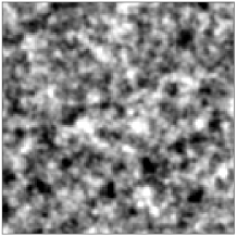
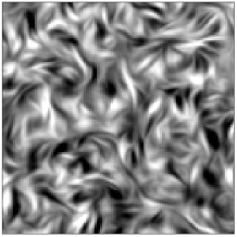
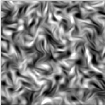
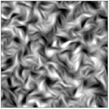
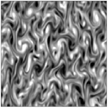
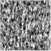
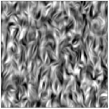
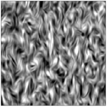
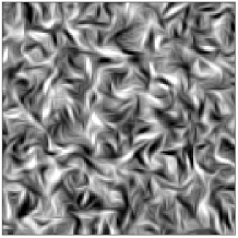
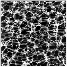
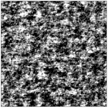
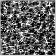
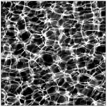
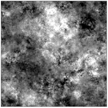
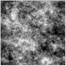
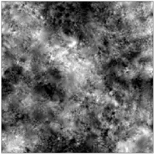
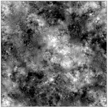
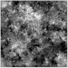
The quality of different microcanonical models is first evaluated visually. Among 10 synthesis of each model, we retain the one which yields the smallest loss in (37). The top row of Figure 5 shows a realization of different stationary processes . The first and second columns display isotropic and non-istotropic vorticity fields of two-dimensional turbulent flows, with a factor 2 zoom on the central part of each image. The third and fourth columns show an image of bubbles and a realization of Multifractal Random Walk [26]. An MRW is a self-similar random process with long range dependencies. We model the increments of MRW, which is a stationary process and limit its maximum correlation scale to . The next rows give realizations of the microcanonical models , , and computed from the same realization shown at the top.
As in Figure 3, the foveal Gaussian model looses most geometric structures. On the contrary the models recover most of this geometry. The model captures the correlations of modulus coefficients across angles whereas the model also impose covariance conditions on phases. There are little visual differences on turbulent flows but it is more apparent on bubble images. Model does not reproduce closed bubbles whereas model recovers bubbles having a better geometry. The model is an isotropic version of model . Its realizations are therefore isotropic. When is isotropic then it is visually as precise as but the variance reduction is not visible. If is not isotropic, as in the turbulence of the second column, then model does not reproduce the angular anisotropy.
5.3 Evaluations of Foveal Covariance Models
A microcanonical model is conditioned by values of the covariance of on a graph whose edges relate neighbor vertices . We differentiate two types of model errors. Type I errors result from the use of graph neighborhoods which are too small. In this case, the covariance of and may be different for . Type II errors are due to the choice of the representation . Such errors are evaluated by comparing high order moments of and , which are not calculated by . These comparisons are performed for .
Wavelet harmonic covariance error
Comparisons are performed over correlation matrices, which normalizes covariance values. Type I errors are calculated by comparing the correlation values of and over a neighborhood which is much larger than the ones used by the different models. This paragraph considers the case where this neighborhood includes all scales and angles, but over a limited spatial range.
We compute correlation coefficients (38) by normalizing with its diagonal:
| (40) |
We estimate with an empirical average over realizations of . This gives an accurate estimation of both and . An empirical estimator of is computed from a single realization of , with the same normalization
It is calculated on where is a foveal subset of all vertices. It incorporates correlations between all scales and angles, across a limited spatial range.
Let be the operator norm and hence the largest eigenvalue of the symmetric matrix restricted to . The following empirical error measures the estimator error of from one realization
| (41) |
It is a variance term due to variabilities of realizations of .
| Isotropic | Non Isotropic | |
|---|---|---|
| 0.58 (0.05) | 0.68 (0.09) | |
| 0.82 (0.01) | 0.80 (0.01) | |
| 0.29 (0.02) | 0.30 (0.02) | |
| 0.24 (0.02) | 0.25 (0.03) | |
| 0.25 (0.02) | 1.6 (0.09) |
This empirical error is compared to the estimation error of computed from the different microcanonical models. Let be the covariance matrix of wavelet harmonic coefficients of a microcanonical model instead of . This matrix is estimated from realizations of . We compare with by using the same normalization. We define by normalizing the with as in (40). The relative error of the model is defined by
| (42) |
This error has a variance term because the microcanonical model depends upon a particular realization of . It has also a bias term because the model is calculated from covariances over a limited set . Optimizing is a trade-off between the variance and bias terms. If the sufficient statistic set is too small and is unable to reproduce the correlations in then is larger than . If then the variance term dominates and .
We define with , , a maximum range of scales and a maximum range of angles , but a small translation range . Its size is , so errors are evaluated over correlation values. Table 1 compares the empirical error in (41) with the model error in (42), for models . We report the mean of these estimated errors by averaging the operator norms over realizations of . The standard deviation is given in brackets. These error values are consistent with visual evaluations.
Table 1 show that the Gaussian model A gives a larger error than , because it captures no dependence across scales and angles. It introduces a large model bias. For models and , . The increase of dramatically reduces the model bias, which clearly appears visually. These models are only conditioned by wavelet harmonic covariances over neighbor scales, but the microcanonical model propagates these constraints across all scales. It provides a good approximation of covariance values between far away scales, evaluated in . The error of model is smaller than model , suggesting that scale correlations through phase also play an important role. This also appears in the visual quality of synthesized bubble images. The model has a similar error as model for the isotropic turbulence although it has a lower variance because estimators are averaged across angular directions. This indicates that the error is dominated by the model bias term and hence that a better model would be obtained by further increasing . This is verified on model by increasing and , which yields a smaller covariance error 0.20 (0.02) on the isotropic turbulence. On the contrary, the model has an error which is much larger than model on the non-isotropic turbulence, which also appears visually.
Long-range spatial correlations
Our microcanonical models are computed with foveal sufficient statistics sets, which are conditioned over relatively small spatial neighborhood at each scale . Such models can therefore introduce a large error if there exists long range spatial correlations between wavelet harmonic coefficients. This paragraph evaluates such errors.
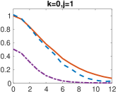
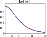
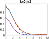
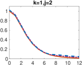
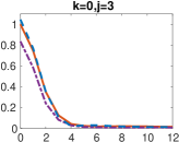
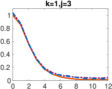
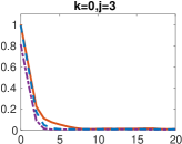
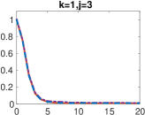
We compare and for and with , and for large . We estimate an average value of over realizations . The difference between and corresponds to a bias error term. For we define and as the maximum values of and over all and all at a distance , for and fixed.
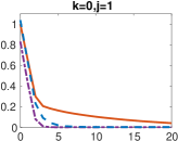
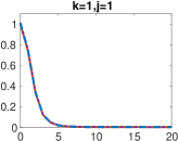
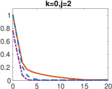
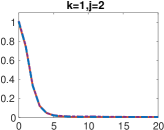
Figure 6 compares the correlation values and as a function of the normalized distance , for and . The notion of short and long range correlations is defined relatively to each scale through the parameter . For , it corresponds to correlations of wavelet coefficients, which have a fast decay when the distance increases. At all scales the long range correlations of wavelet coefficients for models and are close to the correlations obtained with the original turbulence and MRW processes.
For , Figure 6 gives the long range correlation of the modulus of wavelet coefficients. It still has a fast decay for the turbulence field but a slow decay for the MRW. The model gives a much better approximation of long range spatial correlations of turbulence than model . However there is a residual error at the finest scale because these foveal models do not capture long range correlations at fine scales. The error is more dramatic for the MRW process where the modulus of wavelet coefficients are correlated over much longer ranges at fine scales. As expected, this evaluation shows that long range correlations at different scales are not fully captured by foveal models which are constrained on a correlation range of the order of at each scale . One could incorporate these long range spatial covariances by increasing but it would increase considerably the model size which is proportional to .
High order moments
Moments of multiple order can be measured with structure functions at different scale [27, 28]. We compute the maximum moment of order of increments between points such that
It is compared with the structure function calculated for each microcanonical model , with an error
Table 2 reports the mean and standard deviation (in brackets) of for the model and model , at two different scales , for the isotropic turbulence. They are estimated over independent realizations . As expected, the errors increase with the order because foveal covariance model only imposes moments of order and . The model creates no significant error on these high-order moments, since the estimated average error is comparable to the estimator standard deviation. It indicates that in this case the covariance terms across scales are sufficient to capture high order moments. On the contrary, the model has significant errors for because it includes no covariance terms across scales and angles. Table 3 reports the value of these errors for the MRW. The errors of model remain below the errors of model but are significant in this case. This is probably due to the fact that the model does not capture well the long range spatial correlations of the MRW, as shown in Figure 6(b). It introduces a large model error which appears in higher order moments.
| q | 1 | 2 | 3 | 4 | 5 |
|---|---|---|---|---|---|
| 0.04 (0.01) | 0.03 (0.02) | 0.05 (0.04) | 0.14 (0.05) | 0.24 (0.05) | |
| 0.01 (0.01) | 0.02 (0.03) | 0.04 (0.05) | 0.06 (0.07) | 0.10 (0.10) | |
| 0.03 (0.02) | 0.03 (0.02) | 0.05 (0.03) | 0.08 (0.05) | 0.14 (0.07) | |
| 0.01 (0.01) | 0.03 (0.03) | 0.04 (0.05) | 0.06 (0.07) | 0.08 (0.09) |
| q | 1 | 2 | 3 | 4 | 5 |
|---|---|---|---|---|---|
| 0.06 (0.02) | 0.04 (0.03) | 0.16 (0.06) | 0.38 (0.06) | 0.60 (0.04) | |
| 0.02 (0.01) | 0.04 (0.03) | 0.05 (0.05) | 0.13 (0.08) | 0.28 (0.09) |
This analysis shows that microcanonical models computed from phase harmonic covariances in foveal neighborhoods capture important non-Gaussian properties. It gives accurate models of large classes of processes such as the turbulence examples. The evaluation methodology with moments is also able to detect model errors. It shows that long range correlations of wavelet harmonic coefficients are not well captured by foveal models. To circumvent this issue without increasing too much the model size, one can capture these long range correlations with another wavelet transform at each scale, which defines a scattering transform [29]. It amounts to cascade several wavelet transforms and non-linearities to define as in a multilayer convolutional neural network. Very good visual texture syntheses have been obtained with covariances of multi-layer convolutional neural network coefficients [30], but their mathematical properties are not understood.
Appendix A Maximum Entropy Wavelet Covariance model
We explain how to compute the Lagrangian multiples of a maximum entropy stationary Gaussian random vector specified by wavelet covariance values, which is used for the model .
To solve the maximum entropy problem, we follow [2] and derive a dual problem to minimize the entropy with respect to the Lagrangian multiples. To simplify the deviation, we assume that is a zero-mean stationary process, and we consider only the translation group . The wavelet transform is indexed by . The maximum-entropy wavelet covariance model can be written
The sum over is real-valued because .
With the Parseval formula, the sum over translations in can be written in the Fourier domain as a sum over frequencies
The power spectrum of is
To find the optimal Lagrange multipliers, we minimize the entropy of with respect to all the dual variables . The entropy has a closed form,
| (43) |
The partition function also has a closed form,
Note that the should be constrained so that . This constrained optimization problem is addressed by setting the entropy loss to infinity if any condition is violated. The derivative of with respect to is calculated from (43). We can thus use an unconstrained optimization solver L-BFGS to solve this problem from the real and imaginary parts of and . The optimal solution gives the power spectrum of the Gaussian model . Samples of model A are obtained by sampling a stationary Gaussian random vector whose power spectrum is .
Appendix B Proof of Theorem 2.1
We show that for the rectifier ,
| (44) |
By definition, . Since , we do the proof on . We prove the theorem by first showing that for a rectifier and any
Indeed and or and . The equality is verified by considering separately the cases where and have same or different signs. For we get
Appendix C Proof of Theorem 2.2
Property (22) is proved similarly to (13) by translating by and by using its stationarity to verify that so both terms vanish if .
Property (25) is verified for by decomposing nominator and denominator with . Property (23) uses the same decomposition and the fact that and
This is proved again by translating by , which transforms into . Since is stationary, it does not modify this expected value and hence . Since this is valid for any , if modulo in dimension .
Property (23) for and property (24) are also proved by decomposing and showing that
| (47) |
This results from the fact that is real so and .
If is Gaussian then and are independent if because they are Gaussian random variables with a zero covariance. It results that and are also independent for any and hence have a zero covariance if . If and then (22) proves that their covariance remains zero. It results that only if and hence that the covariance is diagonalized. If then is a zero-mean complex Gaussian random variable whose real and imaginary parts are not correlated. As a result .
Appendix D Bump Steerable wavelet
We review the bump steerable wavelet introduced in [3]. It is illustrated in Figure 1 and provides a sparse representation of images with oriented structures. A general way of constructing steerable wavelets is to use the polar coordinate in the Fourier frequency domain [15].
We specify the bump steerable wavelet along the radius and angle for . We assume that the number of angles is even and its central frequency is . Its formula is
where is a normalization constant. The radial function along is a bump function which is a compact-support approximation of a Gaussian window. The same angular window function along is used in [14].
As in [3], the father wavelet is an isotropic Gaussian window function,
We choose , and . These hyper-parameters are also used in [3]. For the wavelet transform with oversampling, we obtain numerically the frame constants and for , and . It is therefore a complete and stable representation. These mother and father wavelets also satisfy and .
Appendix E Proof of Theorem 4.1
Observe first that is invariant to the action of any . Indeed, the probability measure of a Gaussian white noise is uniform on an ball of centered in . As a result is invariant to the action of any linear unitary operator and hence invariant to the action of any which is linear and unitary. Since is invariant to the action of , if the gradient descent is covariant to the action of then the derivations of Theorem 3.4 in [10] prove that the probability measure of is invariant to for .
We thus need to show that the L-BFGS gradient-descent algorithm is covariant to the action at each iteration (before stopped by line-search conditions). Let and be two sequences generated by the gradient descent from the initial conditions and . The covariance to the action of means that if then for any . Although invariant properties of a gradient-based algorithm are well studied in the optimization literature [24, 31], we give below a prove for completeness.
L-BFGS is a variant of the quasi-Newton method BFGS. It estimates the inverse Hessian matrix of the objective function based on
Assume there is a limited memory size to compute an approximation of the Hessian, from and for . At each iteration , the algorithm chooses an appropriate step-size satisfying strong Wolfe conditions [24] and updates with
Since and , it results that . It implies that
| (48) |
We prove the covariance property by induction. We suppose that for in order to prove that . By definition,
The induction assumption implies that and for . It is therefore sufficient to verify that
Each is defined recursively by
for and for all
We thus have . By convention, and for . We thus conclude that . Note that if , the index is negative, and in this case and .
To verify that , we observe that the strong Wolfe-line search conditions are invariant to any linear unitary . Indeed these conditions are invariant to any affine operator [24].
Appendix F Proof of Proposition 5.1
If is invariant to an action of then and are not modified if is transformed into . Similarly, we verify from (3) and (4) that and are not modified if is transformed into . The proposition results are obtained by relating with and applying this relation to and .
(i). If then
| (49) |
For we thus derive that and and thus vanish if is odd. Similarly, for we verify that and which vanishes if is odd.
(ii) If then
| (50) |
because and is real. Since is real, is real. The same property applies to . Applying (50) to and also proves that they are real.
Appendix G Proof of Theorem 5.1
Since the index of can be written . We compute the covariance for with . Since the distribution is stationary the covariance value remains the same if we set .
To prove the theorem we first observe that if then
| (51) |
If is isotropic then and are invariant by rotations. The covariance property (51) thus implies that they are a function of the difference of angles . It is therefore a periodic convolution kernel along angles. It results that the angular dependence is diagonalized by a Fourier transform along the angle variable, which proves (39) for .
A central reflection is a rotation by . Since the distribution of is invariant to all rotations it is invariant to a central reflection. Property (ii) of Proposition (5.1) implies that is real.
Let us consider the line reflection relatively to the horizontal axis. Since and we verify that for any and we have
| (52) |
As a result, if then
| (53) |
If is invariant to line reflections then (53) implies that is not modified when is transformed into . Since is real and invariant to a change of sign of it results that the Fourier coefficients of are also real.
References
- [1] Jaynes, E. T. Information theory and statistical mechanics. Physical review, 106(4):620, 1957.
- [2] Cover, T. M and Thomas, J. A. Elements of Information Theory. Wiley-Interscience, New York, NY, USA, 2006.
- [3] Mallat, S, Zhang, S, and Rochette, G. Phase harmonic correlations and convolutional neural networks. Information and Inference: A Journal of the IMA, 9(3):721–747, 2020.
- [4] Wendt, H, Abry, P, and Jaffard, S. Bootstrap for empirical multifractal analysis. IEEE Signal Processing Magazine, 24(4):38–48, July 2007.
- [5] Farge, M, Schneider, K, and Kevlahan, N. Non-gaussianity and coherent vortex simulation for two-dimensional turbulence using an adaptive orthogonal wavelet basis. Physics of Fluids, 11(8):2187–2201, 1999.
- [6] Grossmann, A, Kronland-Martinet, R, and Morlet, J. Reading and Understanding Continuous Wavelet Transforms. In Combes, J.-M, Grossmann, A, and Tchamitchian, P, editors, Wavelets. Time-Frequency Methods and Phase Space, page 2, 1989.
- [7] Portilla, J and Simoncelli, E. P. A parametric texture model based on joint statistics of complex wavelet coefficients. International Journal of Computer Vision, 40(1):49–70, Oct 2000.
- [8] Ustyuzhaninov, I, Brendel, W, Gatys, L, and Bethge, M. What does it take to generate natural textures? In International Conference on Learning Representations, Apr 2017.
- [9] Lustig, R. Microcanonical monte carlo simulation of thermodynamic properties. The Journal of Chemical Physics, 109(20):8816–8828, 1998.
- [10] Bruna, J and Mallat, S. Multiscale sparse microcanonical models. Mathematical Statistics and Learning, 1:257––315, 2018.
- [11] Zhu, S. C, Wu, Y. N, and Mumford, D. Minimax entropy principle and its application to texture modeling. Neural Computation, 9(8):1627–1660, 1997.
- [12] Cramér, H. Mathematical Methods of Statistics (PMS-9). Princeton University Press, 1999.
- [13] Rao, T. S and Gabr, M. An introduction to bispectral analysis and bilinear time series models, volume 24. Springer Science & Business Media, 2012.
- [14] Simoncelli, E. P and Freeman, W. T. The steerable pyramid: a flexible architecture for multi-scale derivative computation. In Proceedings., International Conference on Image Processing, volume 3, pages 444–447 vol.3, Oct 1995.
- [15] Unser, M and Chenouard, N. A unifying parametric framework for 2d steerable wavelet transforms. SIAM Journal on Imaging Sciences, 6(1):102–135, 2013.
- [16] Mallat, S. A Wavelet Tour of Signal Processing: The Sparse Way, 3rd Edition. Academic Press, 2001.
- [17] Schneider, K, Ziuber, J, Farge, M, and Azzalini, A. Coherent vortex extraction and simulation of 2d isotropic turbulence. Journal of Turbulence, (7):N44, 2006.
- [18] Andreux, M. Foveal Autoregressive Neural Time-Series Modeling. PhD thesis, École normale supérieure, 2018.
- [19] Bortoli, V. D, Desolneux, A, Galerne, B, and Leclaire, A. Macrocanonical models for texture synthesis. In Proc. of Int. Conf. on scale Space and Variational Methods in Computer vision, pages 13–24, Hofgeismar, Germany, 2019.
- [20] Dembo, A and Zeitouni, O. Large Deviations Techniques and Applications. Johns and Bartett Publishers, Boston, 1993.
- [21] Deuschel, J, Stroock, D, and Zession, H. Microcanonical distributions for lattice gases. Commun. Math. Phys., 139:83–101, 1991.
- [22] Georgii, H.-O. Gibbs measures and phase transitions, volume 9. Walter de Gruyter, 2011.
- [23] Lustig, R. Microcanonical monte carlo simulation of thermodynamic properties. The Journal of Chemical Physics, 109(20):8816–8828, 1998.
- [24] Nocedal, J and Wright, S. J. Numerical Optimization. Springer, New York, NY, USA, second edition, 2006.
- [25] Mallat, S. Foveal detection and approximation for singularities. Applied and Computational Harmonic Analysis, 14(2):133–180, 2003.
- [26] Bacry, E, Delour, J, and Muzy, J.-F. Multifractal random walk. Physical Review E, 64(2):026103, 2001.
- [27] Van’Yan, P. Structure function of the velocity field in turbulent flows. Journal of Experimental and Theoretical Physics, 82(3):580–586, 1996.
- [28] Farge, M, Kevlahan, N, Perrier, V, and Schneider, K. Turbulence analysis, modelling and computing using wavelets. Wavelets in Physics, pages 117–200, 1999.
- [29] Leonarduzzi, R, Rochette, G, Bouchaud, J.-P, and Mallat, S. Maximum-entropy Scattering Models for Financial Time Series. In Proc. ICASSP, pages 5496–5500, 2019.
- [30] Gatys, L, Ecker, A. S, and Bethge, M. Texture synthesis using convolutional neural networks. In Advances in Neural Information Processing Systems, pages 262–270, 2015.
- [31] Fletcher, R. Practical Methods of Optimization, 2nd Edition. Wiley-Interscience, New York, NY, USA, 1987.